Embed Size (px)
Citation preview

Chapter Thirteen Soil Lateral Earth Pressure
1
Chapter 13: Lateral Earth Pressure
Retaining structures such as retaining walls, basement walls, and bulkheads
commonly are encountered in foundation engineering as they support slopes of
earth masses. Proper design and construction of these structures require a
thorough knowledge of the lateral forces that act between the retaining
structures and the soil masses being retained. These lateral forces are caused by
lateral earth pressure. This chapter is devoted to the study of the earth pressure
theory.
13.1 At-Rest, Active, and Passive Pressures
Consider a mass of soil shown in Figure 13.1a. The mass is bounded by a
frictionless wall of height AB. A soil element located at a depth z is subjected to
a vertical effective pressure, , and a horizontal effective pressure, . There
are no shear stresses on the vertical and horizontal planes of the soil element.
Let the ratio of , to , as a nondimensional quantity K, or
K
(13.1)
Now, three possible cases may arise concerning the retaining wall: and they
are described
Case 1 If the wall AB is static—that is, if it does not move either to the right or
to the left of its initial position—the soil mass will be in a state of static
equilibrium. In that case, is referred to as the at-rest earth pressure, or
(13.2)
where = at-rest earth pressure coefficient.
Case 2 If the frictionless wall rotates sufficiently about its bottom to a position
of (Figure 13.1b), then a triangular soil mass adjacent to the wall will
reach a state of

Chapter Thirteen Soil Lateral Earth Pressure
2
Figure 13.1 Definition of at-rest, active, and passive pressures (Note: Wall AB is frictionless)
plastic equilibrium and will fail sliding down the plane . At this time, the
horizontal effective stress,
, will be referred to as active pressure. Now,
(13.3)
where = active earth pressure coefficient.
Case 3 If the frictionless wall rotates sufficiently about its bottom to a position
(Figure 13.1c), then a triangular soil mass will reach a state of
plastic equilibrium and will fail sliding upward along the plane . The

Chapter Thirteen Soil Lateral Earth Pressure
3
horizontal effective stress at this time will be
, the so-called passive
pressure. In this case,
(13.4)
13.2 Earth Pressure at-Rest
The fundamental concept of earth pressure at rest was discussed in the preceding
section. In order to define the earth pressure coefficient Ko at rest, we refer to
Figure 13.2. Which shows a wall AB retaining a dry soil with a unit weight of .
The wall is static. At a depth z,
Vertical effective stress =
Horizontal effective stress =
So,
For coarse-grained soils, the coefficient of earth pressure at rest can be
estimated by using the empirical relationship (Jaky, 1944)
(13.5)
Where = drained friction angle.
Figure 13.2 Earth pressure at rest

Chapter Thirteen Soil Lateral Earth Pressure
4
Mayne and Kulhawy (1982), after evaluating 171 soils, recommended a
modification to Eq. (13.5). Or
(13.6)
where
Equation (13.6) is valid for soils ranging from clay to gravel.
For fine-grained, normally consolidated soils, Massarsch (1979) suggested the
following equation for Ko:
(13.7)
For overconsolidated clays, the coefficient of earth pressure at rest can be
approximated as
(13.8)
Figure 13.3 shows the distribution of lateral earth pressure at rest on a wall of
height H retaining a dry soil having a unit weight of . The total force per unit
length of the wall, Po, is equal to the area of the pressure diagram, so
(13.9)
Figure 13.3 Distribution of lateral earth pressure at-rest on a wall

Chapter Thirteen Soil Lateral Earth Pressure
5
13.3 Rankine’s Theory of Active Pressure
The phrase plastic equilibrium in soil refers to the condition where every point
in a soil mass is on the verge of failure. Rankine (1857) investigated the stress
conditions in soil at a state of plastic equilibrium. In this section and in Section
13.4, we deal with Rankine’s theory of earth pressure.
Figure 13.4a shows a soil mass that is bounded by a frictionless wall, AB, that
extends to an infinite depth. The vertical and horizontal effective principal
stresses on a soil element at a depth z are and
respectively. As we saw in
Section 13.2, if the wall AB is not allowed to move, then
. The stress
condition in the soil element can be
13.4 Rankine’s active earth Pressure

Chapter Thirteen Soil Lateral Earth Pressure
6
represented by the Mohr’s circle a in Figure 13.4b. However, if the wall AB is
allowed to move away from the soil mass gradually, the horizontal principal
stress will decrease. Ultimately a state will be reached when the stress condition
in the soil element can be represented by the Mohr’s circle b, the state of plastic
equilibrium and failure of the soil will occur. This situation represents Rankine’s
active state, and the effective pressure on the vertical plane (which is a
principal plane) is Rankine’s active earth pressure. We next derive in terms
of from Figure 13.4b
But
and
So,
or
or
(13.10)
But
and

Chapter Thirteen Soil Lateral Earth Pressure
7
Substituting the preceding values into Eq. (13.10), we get
(13.11)
The variation of with depth is shown in Figure 13.4c. For cohesionless soils,
and
(13.12)
The ratio of to
is called the coefficient of Rankine’s active earth pressure
and is given by
(13.13)
Again, from Figure 13.4b we can see that the failure planes in the soil make
degree angles with the direction of the major principal plane that is,
the horizontal. These are called potential slip planes and are shown in Figure
13.4d.
It is important to realize that a similar equation for could be derived
based on the total stress shear strength parameters that is, . For
this case,
(13.14)
13.4 Theory of Rankine’s Passive Pressure
Rankine’s passive state can be explained with the aid of Figure 13.5. AB is a
frictionless wall that extends to an infinite depth (Figure 13.5a). The initial stress
condition on a soil element is represented by the Mohr’s circle a in Figure 13.5b.
If the wall gradually is pushed into the soil mass, the effective principal stress
will increase. Ultimately, the wall will reach a situation where the stress
condition for the soil element can be expressed by the Mohr’s circle b. At this
time, failure of the soil will occur. This situation is referred to as Rankine’s
passive state. The lateral earth pressure , which is the major principal stress, is
called Rankine’s passive earth pressure. From Figure 13.5b, it can be shown
that

Chapter Thirteen Soil Lateral Earth Pressure
8
(13.15)
The derivation is similar to that for Rankine’s active state.
Figure 13.5c shows the variation of passive pressure with depth. For
cohesionless soils ( ),
or
(13.16)
Kp (the ratio of effective stresses) in the preceding equation is referred to as the
coefficient of Rankine’s passive earth pressure.
13.5 Rankine’s passive earth Pressure

Chapter Thirteen Soil Lateral Earth Pressure
9
13.5(continued)

Chapter Thirteen Soil Lateral Earth Pressure
10
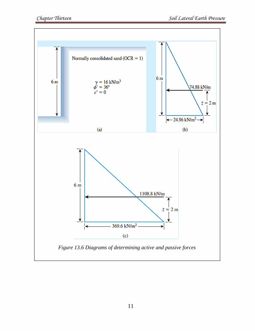
Example 13.1
An 6 m high retaining wall is shown in Figure 13.6a. Determine
a. Rankine active force per unit length of the wall and the location of the
resultant.
b. Rankine passive force per unit length of the wall and the location of the
resultant.
Solution
Part a
Because , to determine the active force we can use from Eq. (13.13).
At z=0, ,
The pressure-distribution diagram is shown in Figure 13.6b. The active force
per unit length of the wall is as follows:
Also,
Part b
To determine the passive force, we are given that . So, from Eq. (13.16),
At z=0, ,
The pressure-distribution diagram is shown in Figure 13.6c. The passive force
unit length of the wall is as follows.
Chapter Thirteen Soil Lateral Earth Pressure
11
Figure 13.6 Diagrams of determining active and passive forces

Chapter Thirteen Soil Lateral Earth Pressure
12
Example 13.2
For the retaining wall shown in Figure 13.7a, determine the force per unit
length of the wall for Rankine’s active state. Also find the location of the
resultant.
Figure 13.7 Retaining wall and pressure diagrams for determining Rankine’s active earth pressure. (Note: The units of pressure in (b), (c), and (d) are kN/m
2)
Solution
Given that , we known that
. For the upper layer of the soil,
Rankine’s active earth pressure coefficient is
For the lower layer,
At z=0,
. So

Chapter Thirteen Soil Lateral Earth Pressure
13
Again, at z=3 m (in the lower layer),
At ,
and
The variation of with depth is shown in Figure 13.7b.
The lateral pressures due to the pore water are as follows.
The variation of u with depth is shown in Figure 13.7c, and that for (total
active pressure) is shown in Figure 13.7d. Thus,
The location of the resultant can be found by taking the moment about the bot-
tom of the wall:

Chapter Thirteen Soil Lateral Earth Pressure
14
Example 13.3
A retaining wall that has a soft, saturated clay backfill is shown in Figure 13.8a.
For the undrained condition ( ) of the backfill, determine
a. Maximum depth of the tensile crack
b. Pa before the tensile crack occurs
c. Pa after the tensile crack occurs
Figure 13.8 Rankine’s active earth pressure due to a soft, saturated clay backfill
Solution
For . From eq. (13.14),
At z=0
At z=6 m
The variation of with depth is shown in Figure 13.8b.
Part a
From the equation;
For cohesive soils ( ), the depth of tensile crack equals:

Chapter Thirteen Soil Lateral Earth Pressure
15
Problems
13.1 Figure 13.9 shows a retaining wall that is restrained from yielding.
Determine the magnitude of the lateral earth force per unit length of the wall.
Also, state the location of the resultant, , measured from the bottom of the wall.
Figure 13.9
Ans.
Part b
Part c

Chapter Thirteen Soil Lateral Earth Pressure
16
13.2 Assume that the retaining wall shown in Figure 13.9 is frictionless.
Determine the Rankine active force per unit length of the wall, the variation of
active earth pressure with depth, and the location of the resultant.
Ans.
13.3 Assume that the retaining wall shown in Figure 13.9 is frictionless.
Determine the Rankine passive force per unit length of the wall, the variation of
lateral earth pressure with depth, and the location of the resultant.
Ans.
13.4 A retaining wall is shown in Figure 13.10. Determine the Rankine active
force, Pa, per unit length of the wall and the location of the resultant.
Ans.
Figure (13.10)

Chapter Thirteen Soil Lateral Earth Pressure
17
13.5 A 5-m-high retaining wall with a vertical back face has a soil for
backfill. For the backfill, , c' = 26 kN/m2, and .
Considering the existence of the tensile crack, determine the active force, Pa, on
the wall for Rankine’s active state.
Ans.