Characteristics of Fish Populations

•

Unexploited Populations–

Recruitment

–

Mortality (natural)–

Growth

•

Exploited Populations–

Recruitment and Yield

–

Fishing and Natural Mortality–

Compensatory Growth

Recruitment and Yield

•

Recruitment is defined as the addition of new members to the aggregate under consideration

•

Generally in fishing the life history stage they are vulnerable to gear

Typical Stocks Harvested

Pre recruitment Post recruitment

Relationships between Recruits and Parents and Sources of

Mortality•

Adult stock numbers can be related to recruits.

•

Two sources of mortality –

–

Density dependent

–

-

Density Independent•

Size and growth characteristics influence production of young

Stock Recruitment

•

Developed using assumption that density dependent mortality

is operating.

Factors that regulate numbers

•

Predation (disease episodes)•

Competition

•

Habitat•

Parent stock abundance

Density Independent Factors

•

Temperatures•

Floods

•

Drought

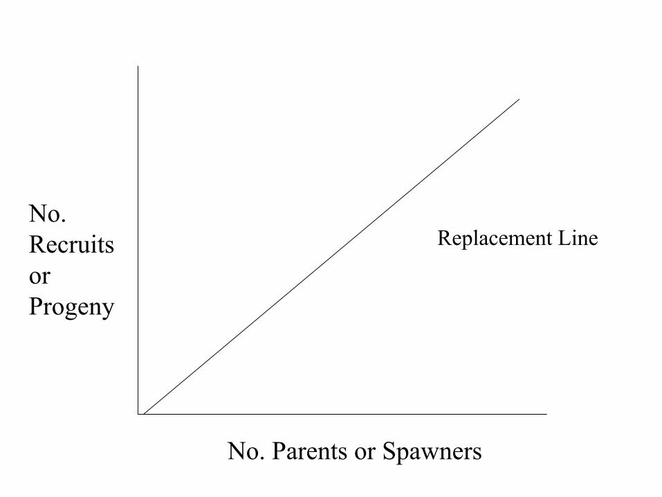
Replacement LineNo. Recruits or Progeny

No. Parents or Spawners

Two Famous Models

•

Developed in 1950s•

Both density dependent driven

•

Ricker & Beverton-Holt

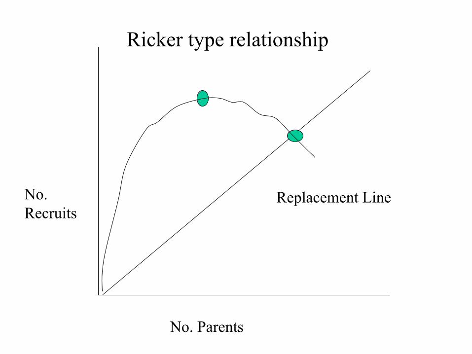
Replacement LineNo. Recruits

No. Parents

Ricker type relationship

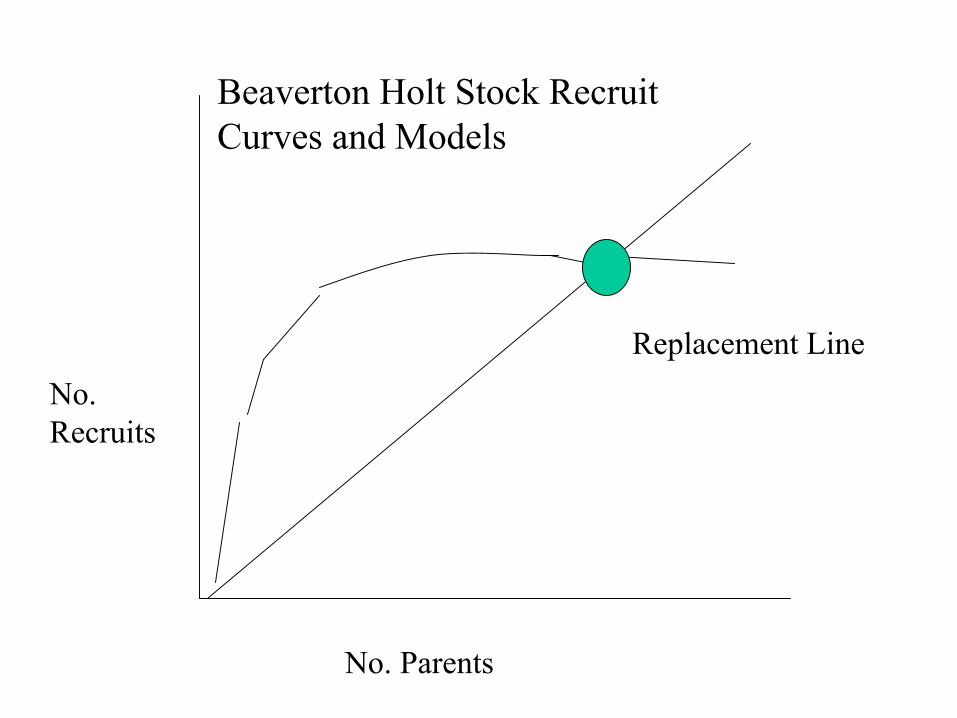
Replacement LineNo. Recruits

No. Parents

Beaverton Holt Stock Recruit Curves and Models

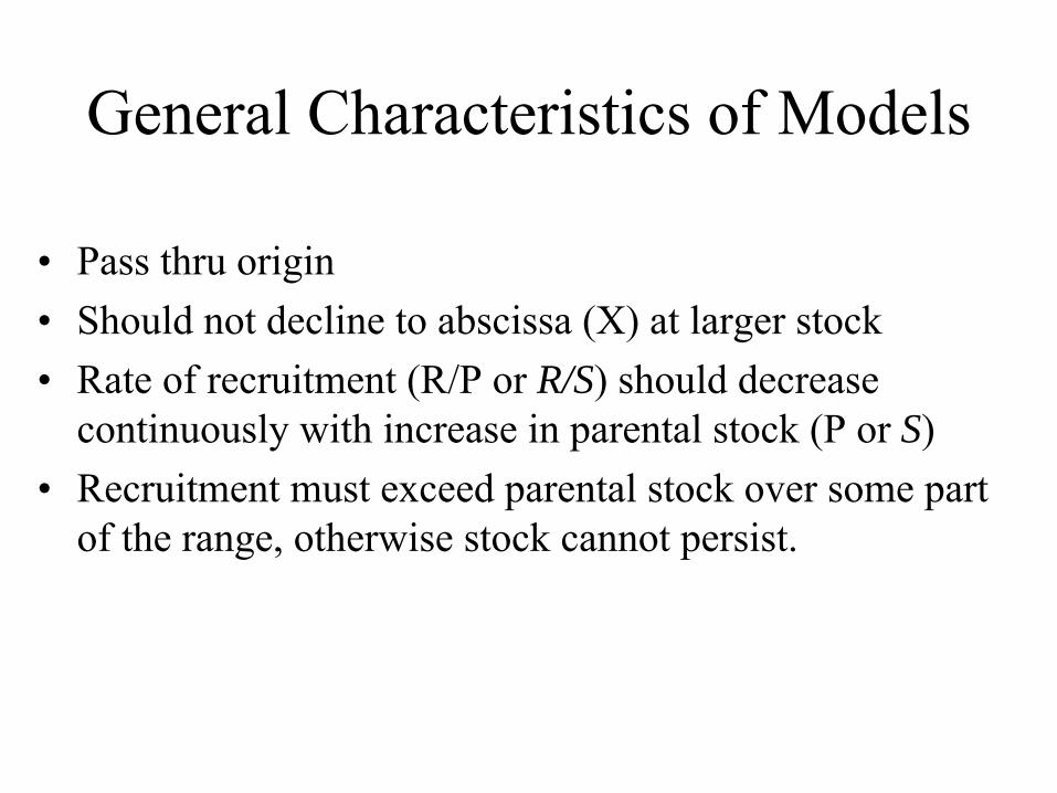
General Characteristics of Models

•

Pass thru origin•

Should not decline to abscissa (X) at larger stock

•

Rate of recruitment (R/P or R/S) should decrease continuously with increase in parental stock (P or S)

•

Recruitment must exceed parental stock over some part of the range, otherwise stock cannot persist.

Recruits

Parents

Replacement Line

A

C0

B0.9

1.2

1.0

Curves and Yields A -

B = surplus production

Theoretical relationship between adult stock and progeny returning as adults

•

Reproduction curve can be expressed as a ratio

•

R/RE

= P/PE

e[Pe-P/Pm]

•

When R is the filial generation P is parent generation PE is equilibrium stock (replacement); Re is filial generation reproduced by PE

and Pm is stock that produces maximum recruitment

•

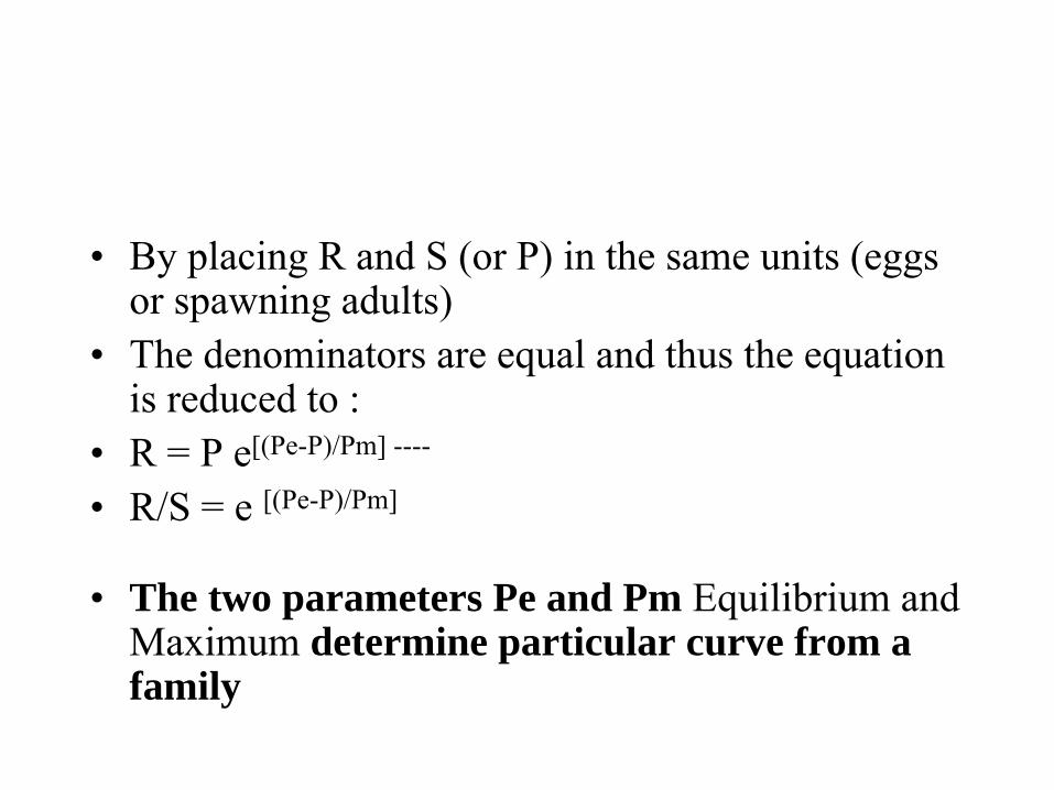
By placing R and S (or P) in the same units (eggs or spawning adults)

•

The denominators are equal and thus the equation is reduced to :

•

R = P e[(Pe-P)/Pm] ----

•

R/S = e [(Pe-P)/Pm]

•

The two parameters Pe and Pm Equilibrium and Maximum

determine particular curve from a

family

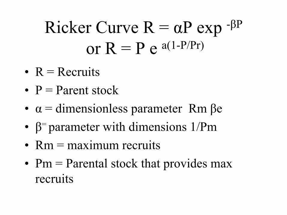
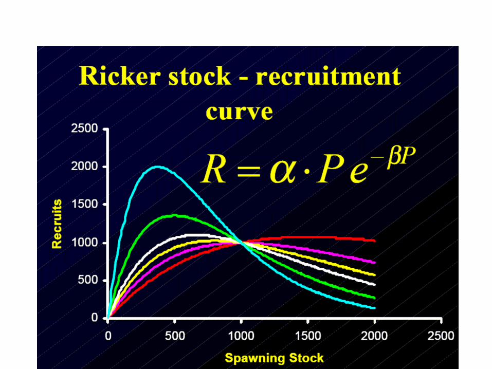
Ricker Curve R = αP exp -βP

or R = P e a(1-P/Pr)

•

R = Recruits •

P = Parent stock

•

α

= dimensionless parameter Rm βe•

β= parameter with dimensions 1/Pm

•

Rm

= maximum recruits•

Pm = Parental stock that provides max recruits

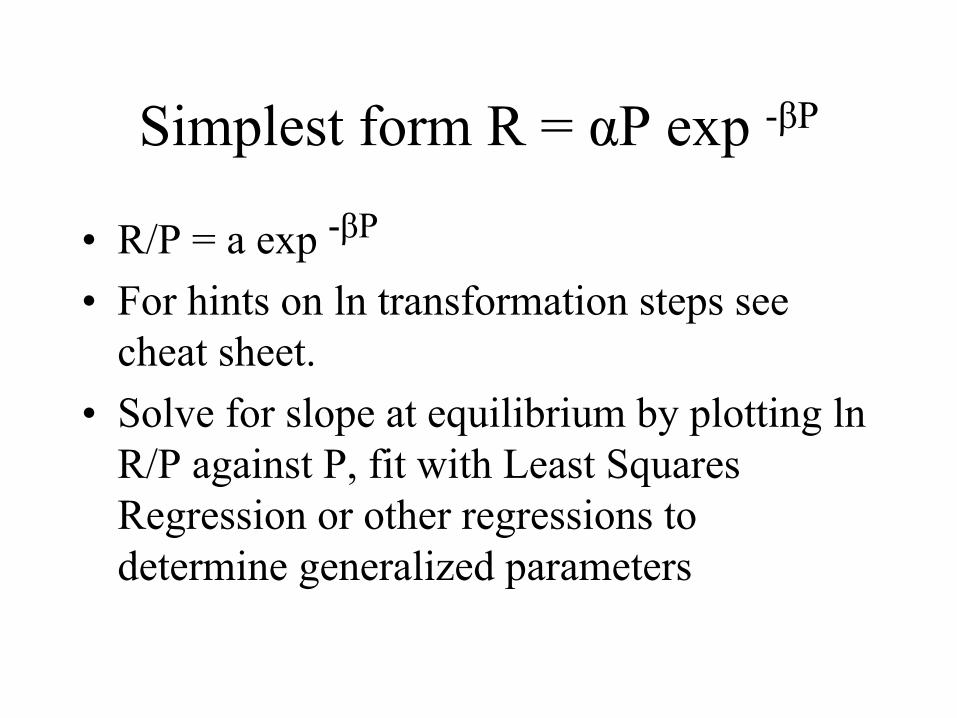
Simplest form R = αP exp -βP

•

R/P = a exp -βP

•

For hints on ln transformation steps see cheat sheet.

•

Solve for slope at equilibrium by plotting

ln R/P against P, fit with Least Squares

Regression or other regressions to determine generalized parameters

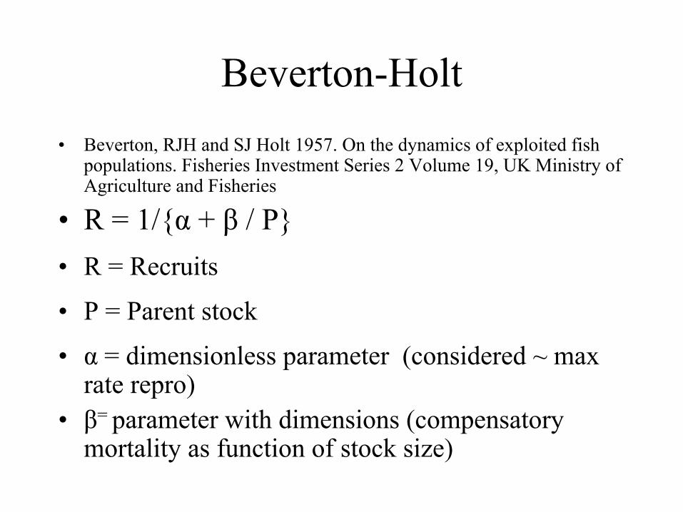
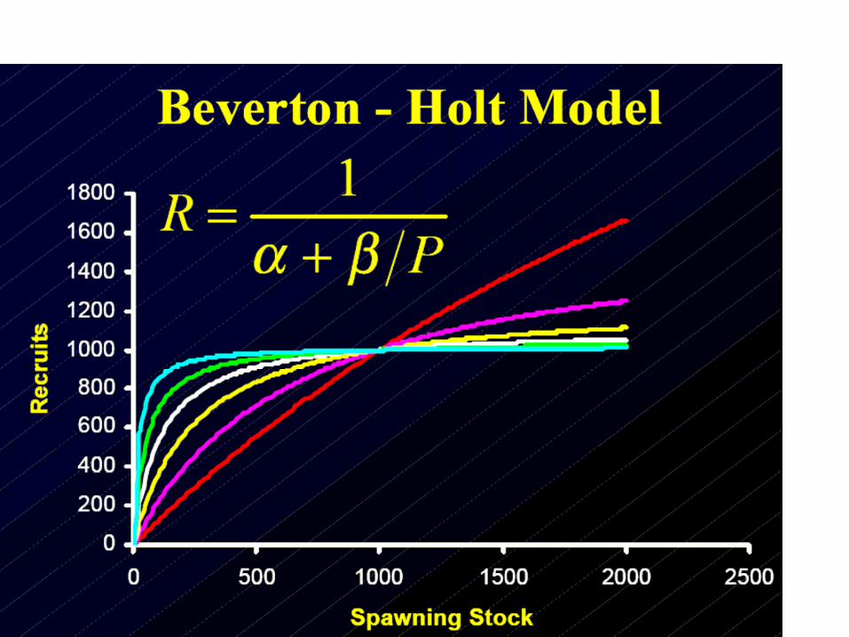
Beverton-Holt•

Beverton, RJH and SJ Holt 1957. On the dynamics of exploited fish populations. Fisheries Investment Series 2 Volume 19, UK Ministry of Agriculture and Fisheries

•

R = 1/{α

+ β

/ P}•

R = Recruits

•

P = Parent stock

•

α

= dimensionless parameter (considered ~ max rate repro)

•

β= parameter with dimensions (compensatory mortality as function of stock size)

Solutions

•

1/R = α

+ β/P

•

P/R = β

+ α

P

•

With either linear solution you estimate 1/R and therefore must correct for this

•Ricker assumed that density- dependence was based on

mobile, aggregating predators

•

Beverton-Holt assumed that predators were always present

Problems with Both

•

Predation can occur in constant rate. If spawning stock becomes very small. They may not be able to produce enough recruits to recover to previous levels

•

Do not account for numbers of

spawners

becoming so low that compensatory mechanisms can no longer occur

•

Inability to find mates (or low fertilization success) with low

broodstock

numbers problems with ecosystem

functions etc.

Simple Case for Exploitation

•

Slope of descending leg determines the type of population cycles that would occur.

•

If population is in descending leg then a slope of –1 will result in undampened oscillations of equal magnitude about the equilibrium point.

•

Slopes between 0 and –1 will cause oscillations about the equilibrium point.

•

Slopes between –1 and –inf will cause oscillations up to the apex of the dome, and then the series of oscillations would be repeated

Multiple age spawning stocks

•

Smaller deflections from equilibrium•

Populations with reproduction curves having descending legs and slopes between 1 and –1 all eventually become stable

Yield or exploitation for desired equilibrium

•

Yield is that portion of a fish population removed by humans

•

Units are generally weight per unit time or unit area

•

Production is the total elaboration of new biomass at the trophic level under consideration generally within some spatial and temporal unit

Recruits

Arbitary units

Parents

Replacement Line

A = surplus equilibrium

C0

B0.9

1.2

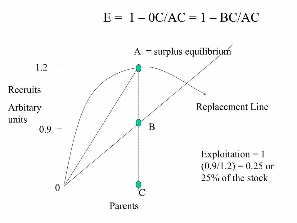
Exploitation = 1 – (0.9/1.2) = 0.25 or

25% of the stock

E = 1 –

0C/AC = 1 –

BC/AC

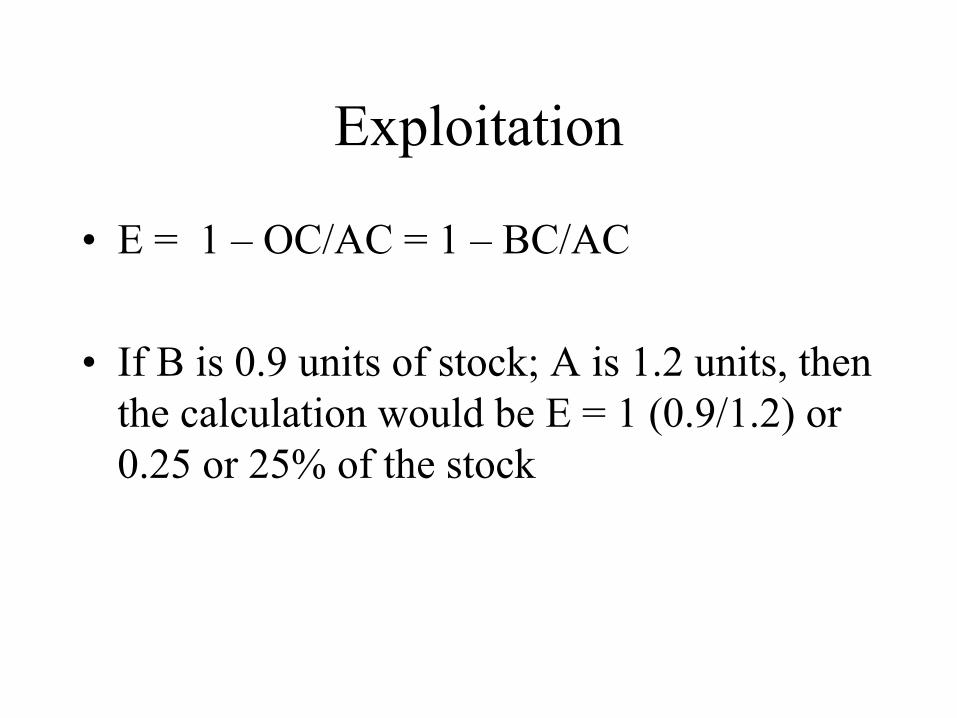
Exploitation

•

E = 1 –

OC/AC = 1 –

BC/AC

•

If B is 0.9 units of stock; A is 1.2 units, then the calculation would be E = 1 (0.9/1.2) or 0.25 or 25% of the stock

Surplus Production

•

The objective of models is to determine the optimum level of effort, that is the effort that produces the maximum yield that can be sustained without affecting me long-term productivity of the stock, the so-called maximum sustainable yield (MSY). The theory behind the surplus production models has been reviewed by many authors, for example, Ricker (1975), Caddy (1980),

Gulland

(1983) and

Pauly

(1984).

Maximum Sustainable yield

•

The highest theoretical equilibrium yield that can be continuously taken (on average) from a stock under existing (average) environmental conditions without affecting significantly the reproduction process.

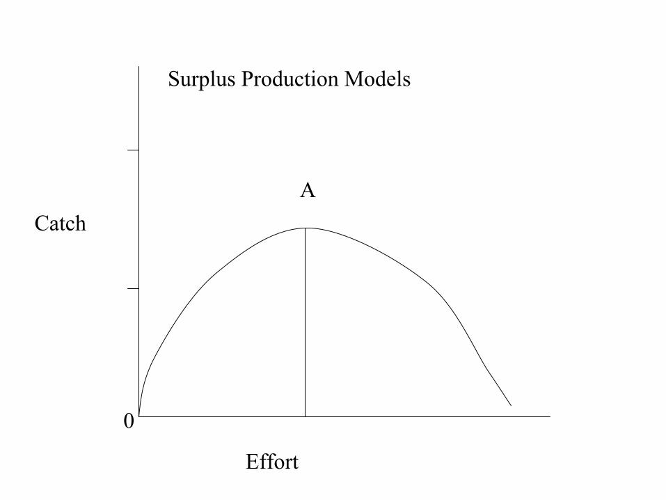
Catch

Effort

A

0

Surplus Production Models

•

For instance, the accuracy of MSY estimates depends upon such measures as rates of growth, mortality, and reproduction that are difficult to determine and that change over time.

•

As a result, scientists generally produce a range of estimates for MSY, based on different assumptions.

Peter Larkin, 1977 An epitaph for the Concept of Maximum

Sustained Yield TAFS 106:1-11MSY 1930s -

1970

Here lies the concept MSYIt advocated yields too highAnd didn’t spell out how to slice the pie.We bury it with the best of wishesEspecially on behalf of fishesWe don’t know yet what will take its place.Be we hope it’s as good for the human race.

R.I.P