Embed Size (px)
Citation preview

1
CISC 4631Data Mining
Lecture 05:• Overfitting• Evaluation: accuracy, precision, recall, ROC
Theses slides are based on the slides by • Tan, Steinbach and Kumar (textbook authors)• Eamonn Koegh (UC Riverside)• Raymond Mooney (UT Austin)
2
Practical Issues of Classification
• Underfitting and Overfitting
• Missing Values
• Costs of Classification
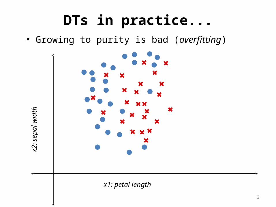
DTs in practice...• Growing to purity is bad (overfitting)
x1: petal length
x2:
sepa
l wid
th
3
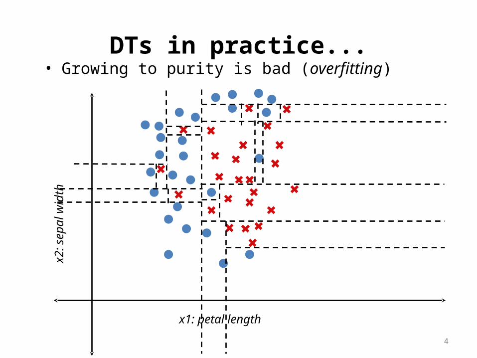
DTs in practice...• Growing to purity is bad (overfitting)
x1: petal length
x2:
sepa
l wid
th
4
5
DTs in practice...
• Growing to purity is bad (overfitting)– Terminate growth early– Grow to purity, then prune back
6
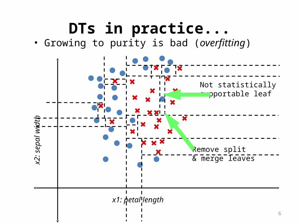
DTs in practice...• Growing to purity is bad (overfitting)
x1: petal length
x2:
sepa
l wid
th
Not statisticallysupportable leaf
Remove split& merge leaves
7
Training and Test Set
• For classification problems, we measure the performance of a model in terms of its error rate: percentage of incorrectly classified instances in the data set.
• We build a model because we want to use it to classify new data. Hence we are chiefly interested in model performance on new (unseen) data.
• The resubstitution error (error rate on the training set) is a bad predictor of performance on new data.
• The model was build to account for the training data, so might overfit it, i.e., not generalize to unseen data.
8
Overfitting
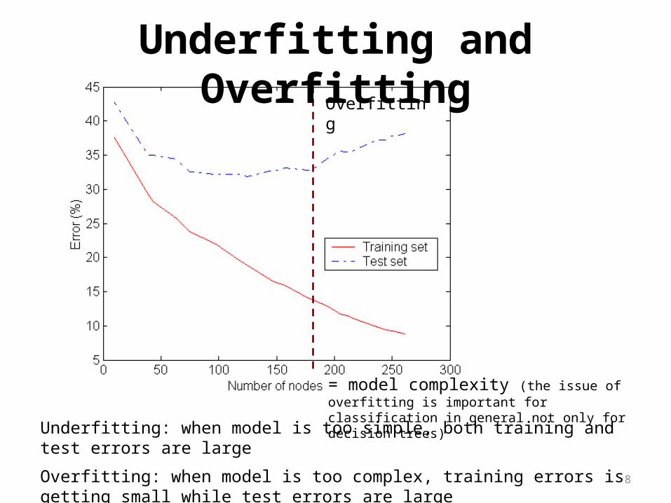
= model complexity (the issue of overfitting is important for classification in general not only for decision trees)
Underfitting and Overfitting
Underfitting: when model is too simple, both training and test errors are large
Overfitting: when model is too complex, training errors is getting small while test errors are large
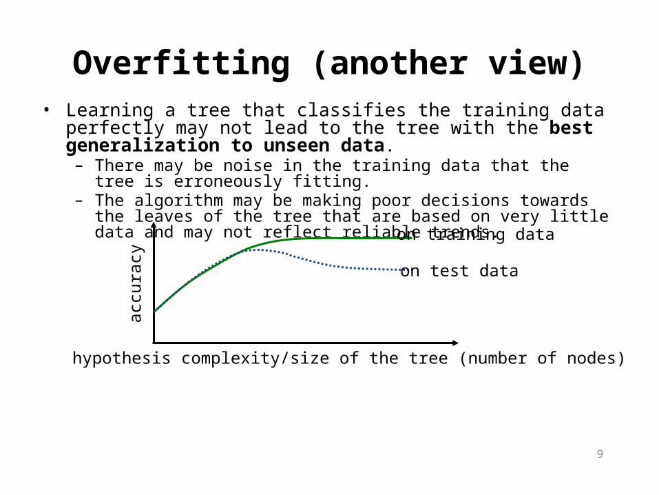
Overfitting (another view)• Learning a tree that classifies the training data perfectly may not lead to
the tree with the best generalization to unseen data.– There may be noise in the training data that the tree is erroneously fitting.– The algorithm may be making poor decisions towards the leaves of the tree
that are based on very little data and may not reflect reliable trends.
hypothesis complexity/size of the tree (number of nodes)
accu
racy
on training data
on test data
9
10
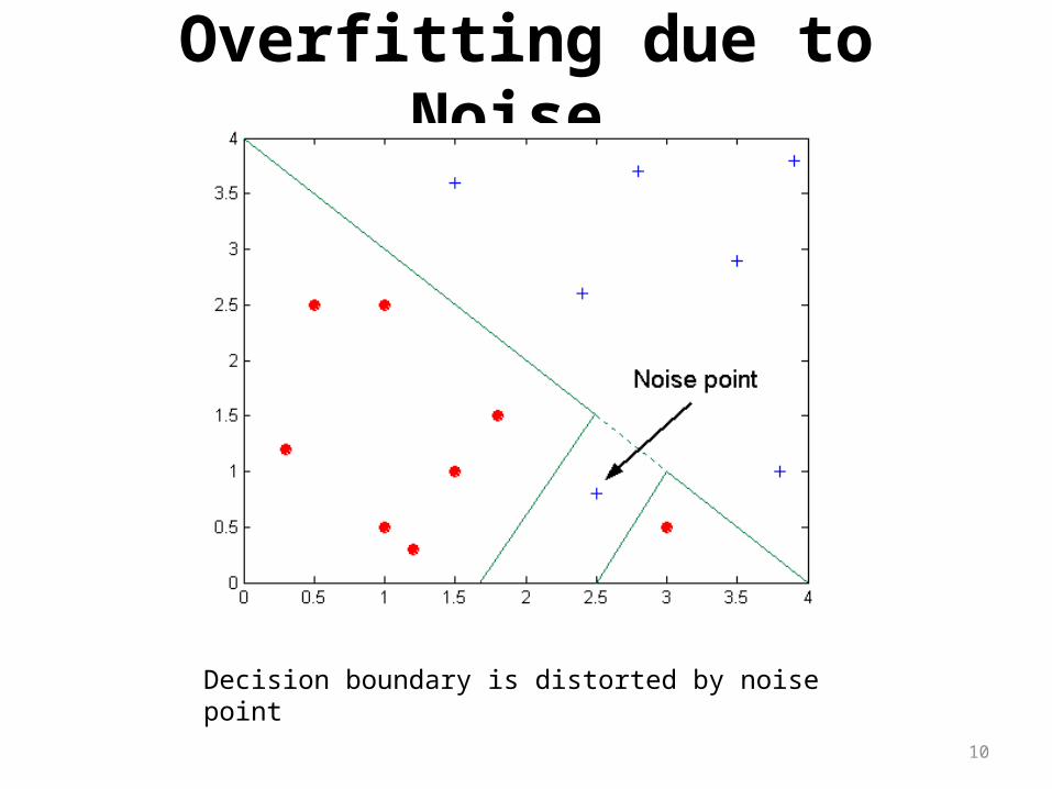
Overfitting due to Noise
Decision boundary is distorted by noise point
11
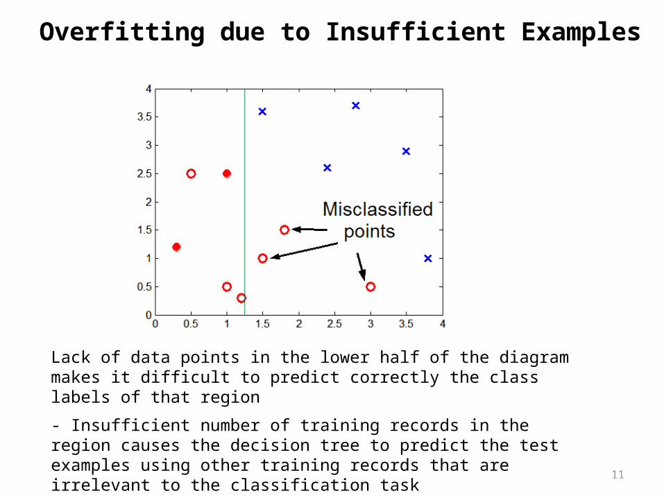
Overfitting due to Insufficient Examples
Lack of data points in the lower half of the diagram makes it difficult to predict correctly the class labels of that region
- Insufficient number of training records in the region causes the decision tree to predict the test examples using other training records that are irrelevant to the classification task
Overfitting Example
voltage (V)
curr
ent (
I)
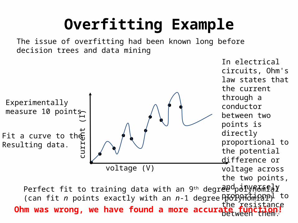
In electrical circuits, Ohm's law states that the current through a conductor between two points is directly proportional to the potential difference or voltage across the two points, and inversely proportional to the resistance between them.
Ohm was wrong, we have found a more accurate function!
Perfect fit to training data with an 9th degree polynomial(can fit n points exactly with an n-1 degree polynomial)
Experimentallymeasure 10 points
Fit a curve to theResulting data.
12
The issue of overfitting had been known long before decision trees and data mining
Overfitting Example
voltage (V)
curr
ent (
I)
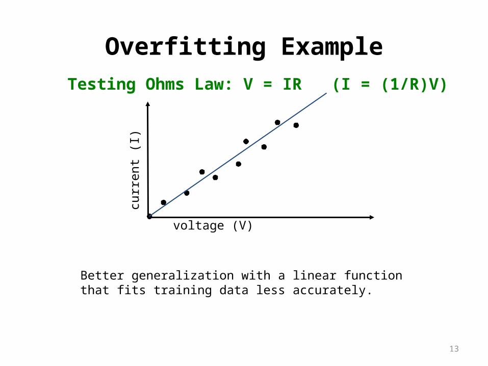
Testing Ohms Law: V = IR (I = (1/R)V)
Better generalization with a linear functionthat fits training data less accurately.
13
14
Notes on Overfitting
• Overfitting results in decision trees that are more complex than necessary
• Training error no longer provides a good estimate of how well the tree will perform on previously unseen records
• Need new ways for estimating errors
How to avoid overfitting?
1. Stop growing the tree before it reaches the point where it perfectly classifies the training data (prepruning)– Such estimation is difficult
2. Allow the tree to overfit the data, and then post-prune the tree (postpruning)– Is used
Although first approach is more direct, second approach found more successful in practice: because it is difficult to estimate when to stop
Both need a criterion to determine final tree size
15
16
Occam’s Razor
• Given two models of similar errors, one should prefer the simpler model over the more complex model
• For complex models, there is a greater chance that it was fitted accidentally by errors in data
• Therefore, one should include model complexity when evaluating a model
17
How to Address Overfitting• Pre-Pruning (Early Stopping Rule)
– Stop the algorithm before it becomes a fully-grown tree– Typical stopping conditions for a node:
• Stop if all instances belong to the same class• Stop if all the attribute values are the same
– More restrictive conditions:• Stop if number of instances is less than some user-specified threshold• Stop if class distribution of instances are independent of the available
features (e.g., using 2 test)• Stop if expanding the current node does not improve impurity
measures (e.g., Gini or information gain).
18
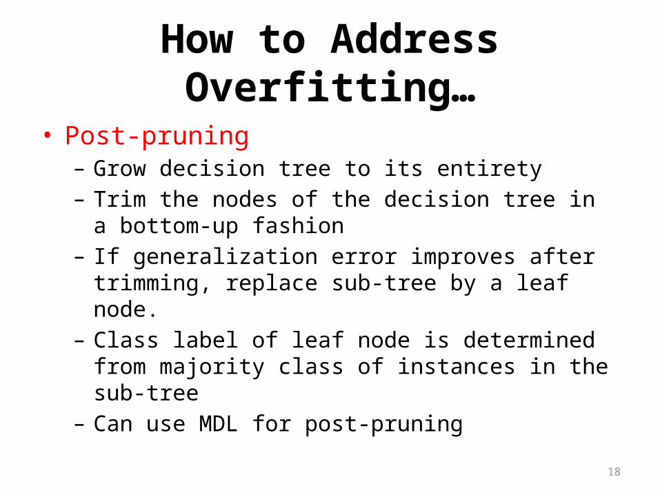
How to Address Overfitting…
• Post-pruning– Grow decision tree to its entirety– Trim the nodes of the decision tree in a bottom-up fashion– If generalization error improves after trimming, replace
sub-tree by a leaf node.– Class label of leaf node is determined from majority class
of instances in the sub-tree– Can use MDL for post-pruning
19
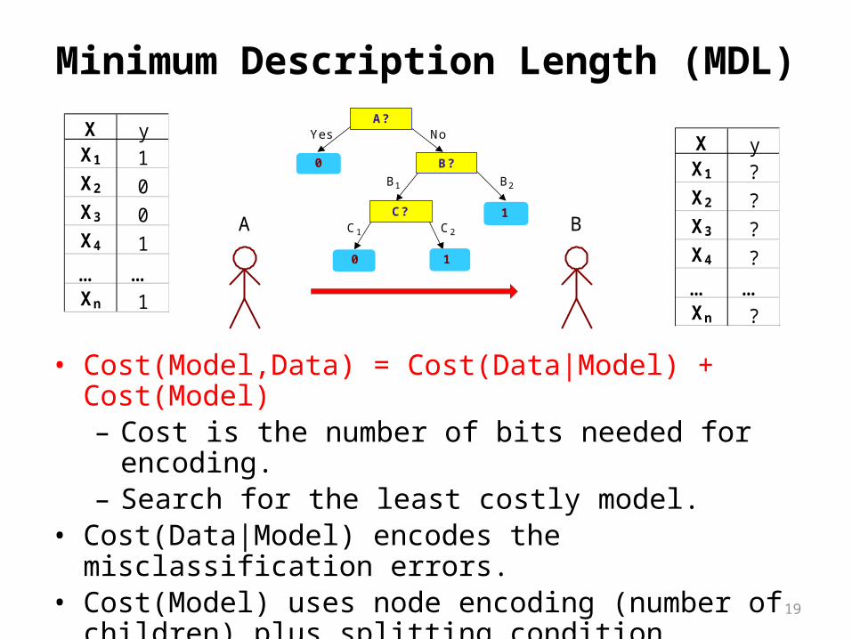
Minimum Description Length (MDL)
• Cost(Model,Data) = Cost(Data|Model) + Cost(Model)– Cost is the number of bits needed for encoding.– Search for the least costly model.
• Cost(Data|Model) encodes the misclassification errors.• Cost(Model) uses node encoding (number of children) plus
splitting condition encoding.
A B
A?
B?
C?
10
0
1
Yes No
B1 B2
C1 C2
X yX1 1X2 0X3 0X4 1
… …Xn 1
X yX1 ?X2 ?X3 ?X4 ?
… …Xn ?
20
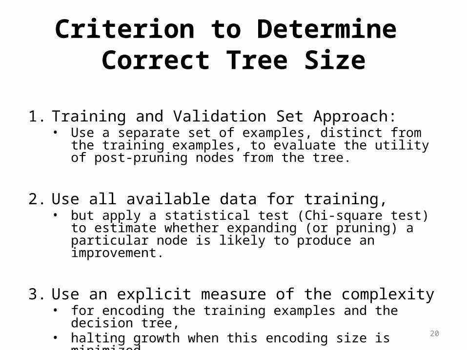
Criterion to Determine Correct Tree Size
1. Training and Validation Set Approach: • Use a separate set of examples, distinct from the training examples,
to evaluate the utility of post-pruning nodes from the tree.
2. Use all available data for training, • but apply a statistical test (Chi-square test) to estimate whether
expanding (or pruning) a particular node is likely to produce an improvement.
3. Use an explicit measure of the complexity• for encoding the training examples and the decision tree,• halting growth when this encoding size is minimized.
21
Validation Set
• Provides a safety check against overfitting spurious characteristics of data
• Needs to be large enough to provide a statistically significant sample of instances
• Typically validation set is one half size of training set• Reduced Error Pruning: Nodes are removed only if the
resulting pruned tree performs no worse than the original over the validation set.
22
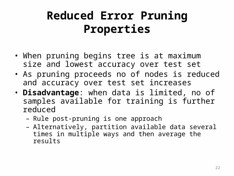
Reduced Error Pruning Properties
• When pruning begins tree is at maximum size and lowest accuracy over test set
• As pruning proceeds no of nodes is reduced and accuracy over test set increases
• Disadvantage: when data is limited, no of samples available for training is further reduced– Rule post-pruning is one approach – Alternatively, partition available data several times in multiple ways
and then average the results
23
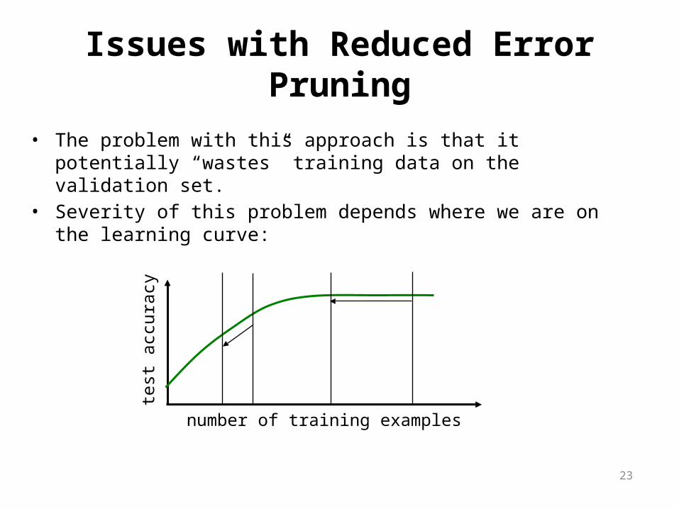
Issues with Reduced Error Pruning
• The problem with this approach is that it potentially “wastes” training data on the validation set.
• Severity of this problem depends where we are on the learning curve:
test
acc
urac
y
number of training examples
24
Rule Post-Pruning (C4.5)
• Convert the decision tree into an equivalent set of rules.• Prune (generalize) each rule by removing any preconditions so
that the estimated accuracy is improved.• Sort the prune rules by their estimate accuracy, and apply
them in this order when classifying new samples.
25
Model Evaluation
• Metrics for Performance Evaluation– How to evaluate the performance of a model?
• Methods for Performance Evaluation– How to obtain reliable estimates?
26
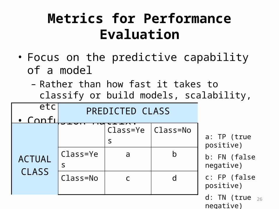
Metrics for Performance Evaluation
• Focus on the predictive capability of a model– Rather than how fast it takes to classify or build models,
scalability, etc.
• Confusion Matrix:PREDICTED CLASS
ACTUALCLASS
Class=Yes Class=No
Class=Yes a b
Class=No c d
a: TP (true positive)
b: FN (false negative)
c: FP (false positive)
d: TN (true negative)
27
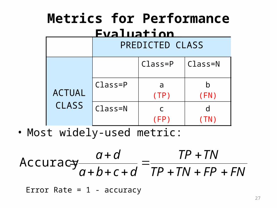
Metrics for Performance Evaluation…
• Most widely-used metric:
PREDICTED CLASS
ACTUALCLASS
Class=P Class=N
Class=P a(TP)
b(FN)
Class=N c(FP)
d(TN)
FNFPTNTPTNTP
dcbada
Accuracy
Error Rate = 1 - accuracy
28
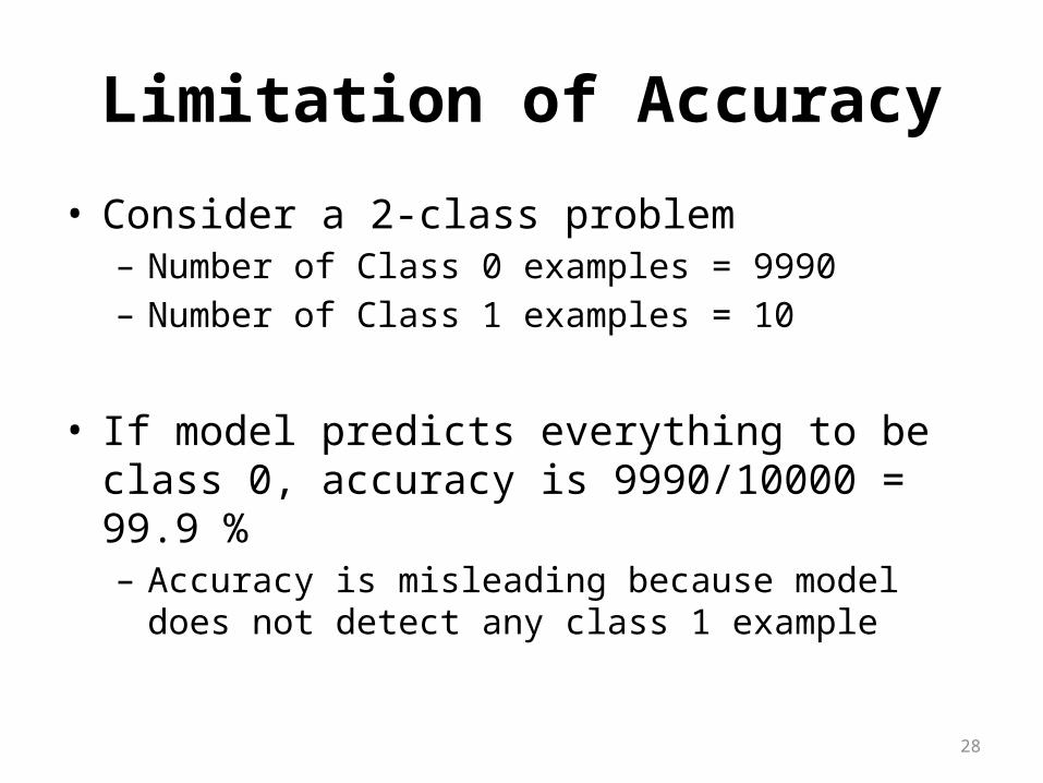
Limitation of Accuracy
• Consider a 2-class problem– Number of Class 0 examples = 9990– Number of Class 1 examples = 10
• If model predicts everything to be class 0, accuracy is 9990/10000 = 99.9 %– Accuracy is misleading because model does not detect any
class 1 example
29
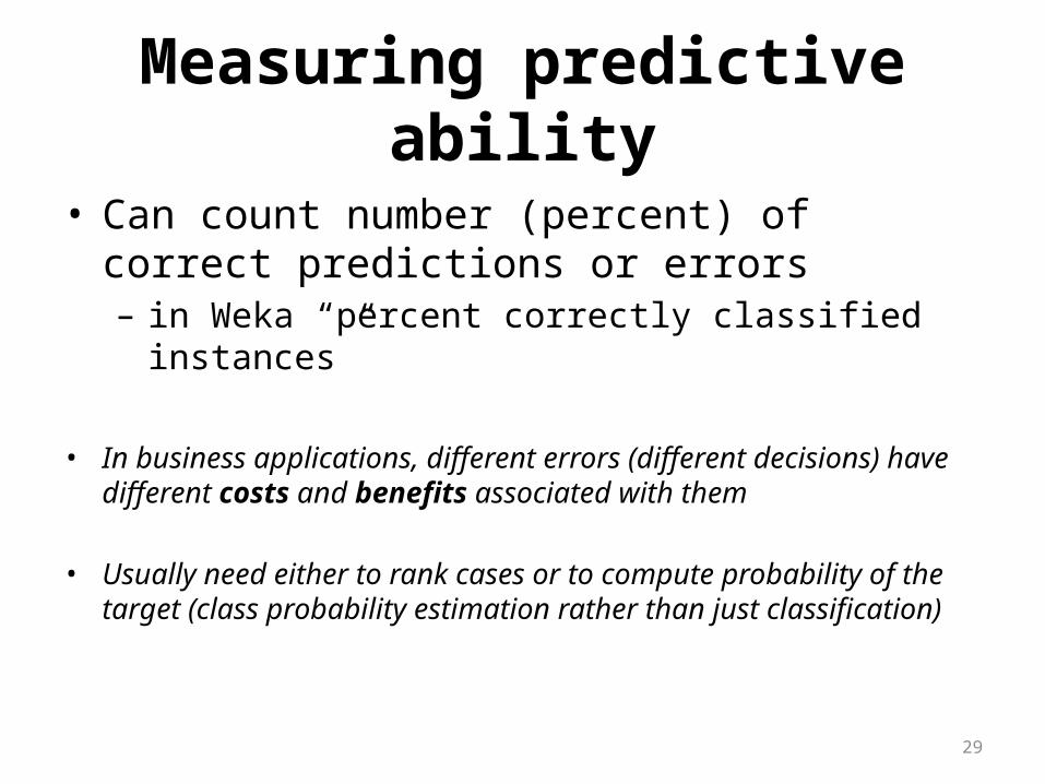
Measuring predictive ability
• Can count number (percent) of correct predictions or errors– in Weka “percent correctly classified instances”
• In business applications, different errors (different decisions) have different costs and benefits associated with them
• Usually need either to rank cases or to compute probability of the target (class probability estimation rather than just classification)
30
Costs Matter
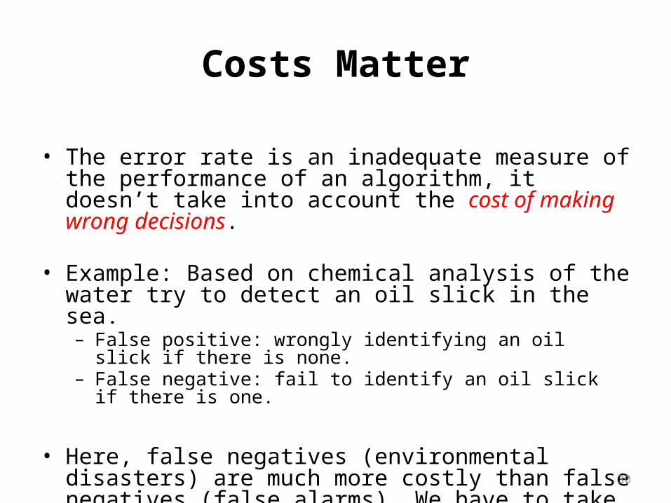
• The error rate is an inadequate measure of the performance of an algorithm, it doesn’t take into account the cost of making wrong decisions.
• Example: Based on chemical analysis of the water try to detect an oil slick in the sea.– False positive: wrongly identifying an oil slick if there is none.– False negative: fail to identify an oil slick if there is one.
• Here, false negatives (environmental disasters) are much more costly than false negatives (false alarms). We have to take that into account when we evaluate our model.
31
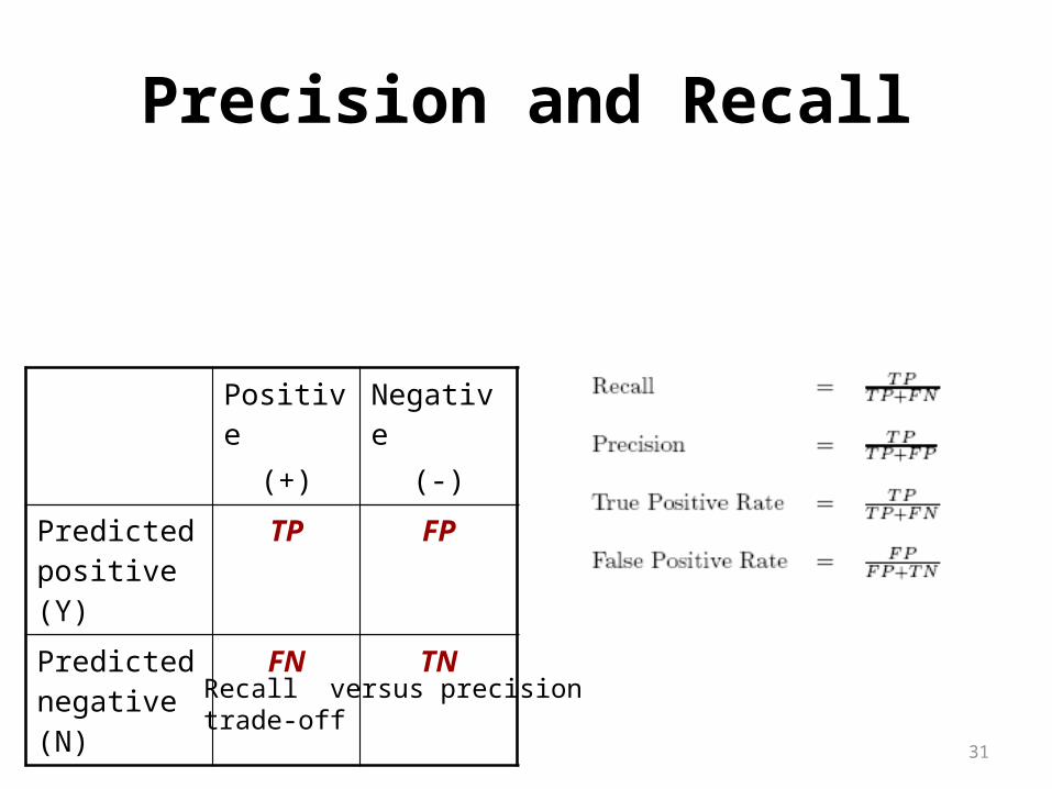
Precision and Recall
Positive(+)
Negative(-)
Predicted positive (Y)
TP FP
Predicted negative (N)
FN TN
Recall versus precision trade-off
32
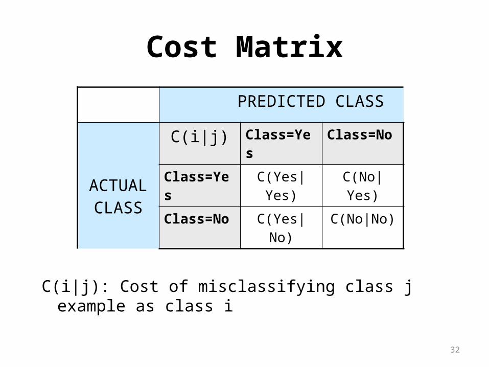
Cost Matrix
PREDICTED CLASS
ACTUALCLASS
C(i|j) Class=Yes Class=No
Class=Yes C(Yes|Yes) C(No|Yes)
Class=No C(Yes|No) C(No|No)
C(i|j): Cost of misclassifying class j example as class i
33
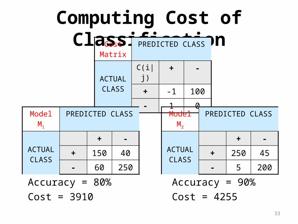
Computing Cost of ClassificationCost
MatrixPREDICTED CLASS
ACTUALCLASS
C(i|j) + -
+ -1 100
- 1 0
Model M1 PREDICTED CLASS
ACTUALCLASS
+ -
+ 150 40
- 60 250
Model M2 PREDICTED CLASS
ACTUALCLASS
+ -
+ 250 45
- 5 200
Accuracy = 80%Cost = 3910
Accuracy = 90%Cost = 4255
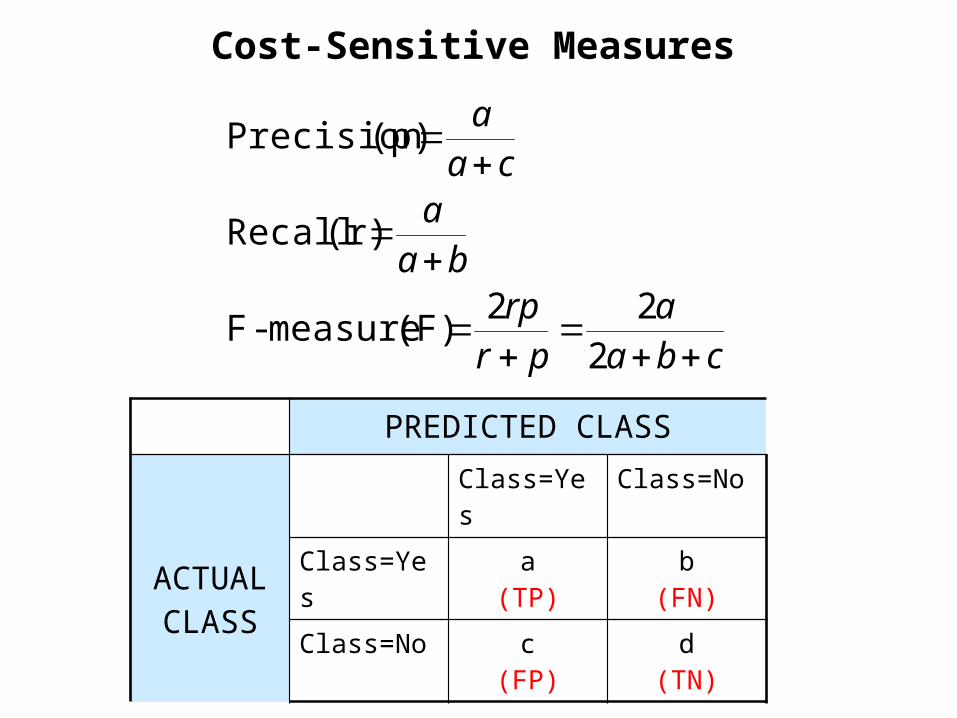
Cost-Sensitive Measures
cbaa
prrp
baa
caa
222
(F) measure-F
(r) Recall
(p)Precision
PREDICTED CLASS
ACTUALCLASS
Class=Yes Class=No
Class=Yes a(TP)
b(FN)
Class=No c(FP)
d(TN)
35
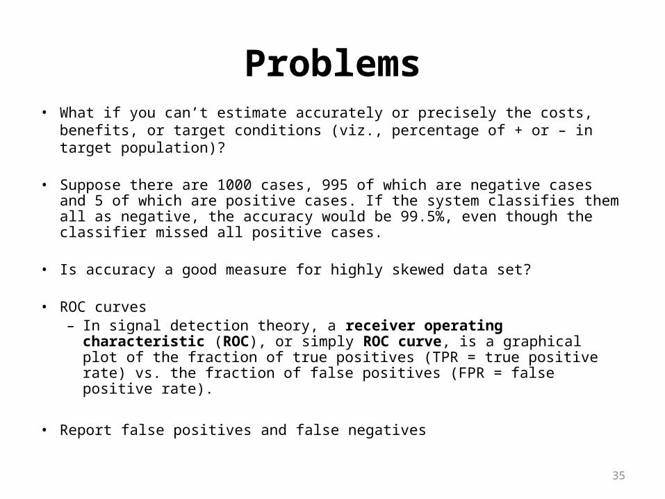
Problems• What if you can’t estimate accurately or precisely the costs, benefits, or
target conditions (viz., percentage of + or – in target population)?
• Suppose there are 1000 cases, 995 of which are negative cases and 5 of which are positive cases. If the system classifies them all as negative, the accuracy would be 99.5%, even though the classifier missed all positive cases.
• Is accuracy a good measure for highly skewed data set?
• ROC curves – In signal detection theory, a receiver operating characteristic (ROC), or
simply ROC curve, is a graphical plot of the fraction of true positives (TPR = true positive rate) vs. the fraction of false positives (FPR = false positive rate).
• Report false positives and false negatives
36
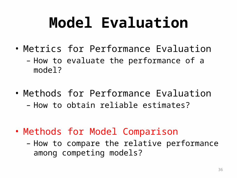
Model Evaluation
• Metrics for Performance Evaluation– How to evaluate the performance of a model?
• Methods for Performance Evaluation– How to obtain reliable estimates?
• Methods for Model Comparison– How to compare the relative performance among
competing models?

37
Classifiers• A classifier assigns an object to one of a predefined
set of categories or classes.• Examples:
– A metal detector either sounds an alarm or stays quiet when someone walks through.
– A credit card application is either approved or denied.– A medical test’s outcome is either positive or negative.
• This talk: only two classes, “positive” and “negative”.
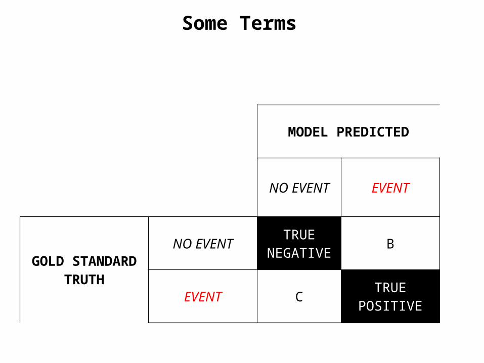
Some Terms
MODEL PREDICTED
NO EVENT EVENT
GOLD STANDARDTRUTH
NO EVENTTRUE
NEGATIVE B
EVENT C TRUE POSITIVE
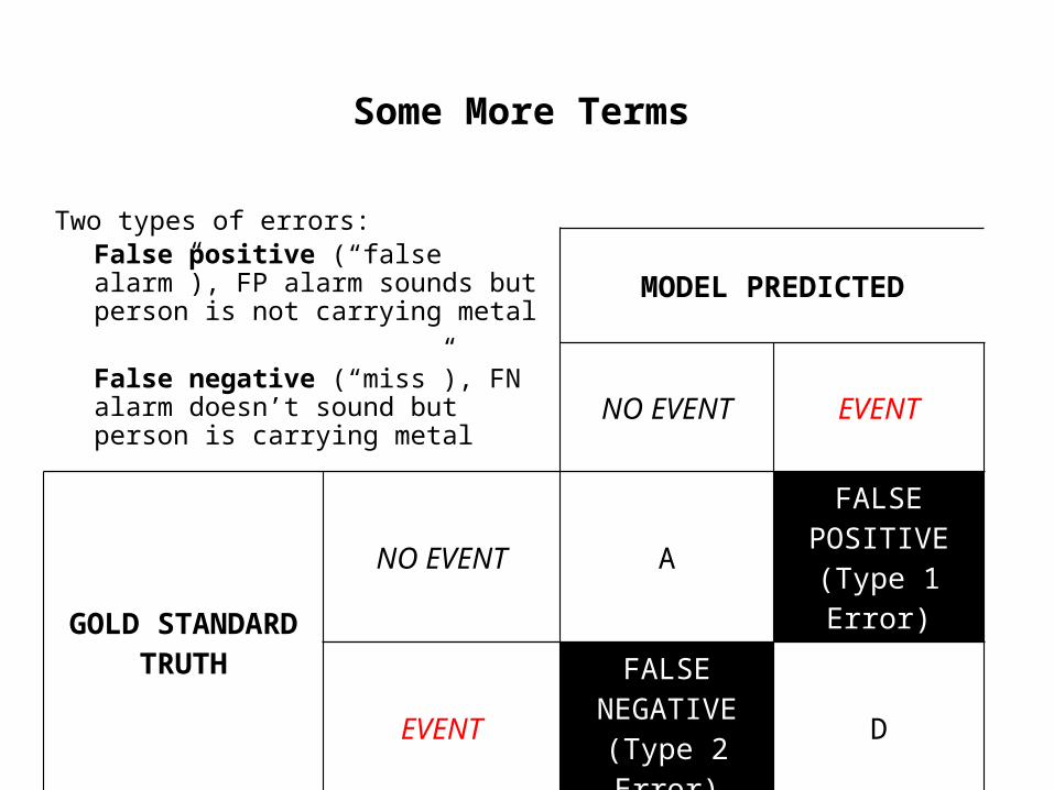
Some More Terms
MODEL PREDICTED
NO EVENT EVENT
GOLD STANDARDTRUTH
NO EVENT AFALSE
POSITIVE(Type 1 Error)
EVENTFALSE
NEGATIVE(Type 2 Error)
D
Two types of errors: False positive (“false alarm”), FP alarm sounds but person is not carrying metal
False negative (“miss”), FN alarm doesn’t sound but person is carrying metal
40
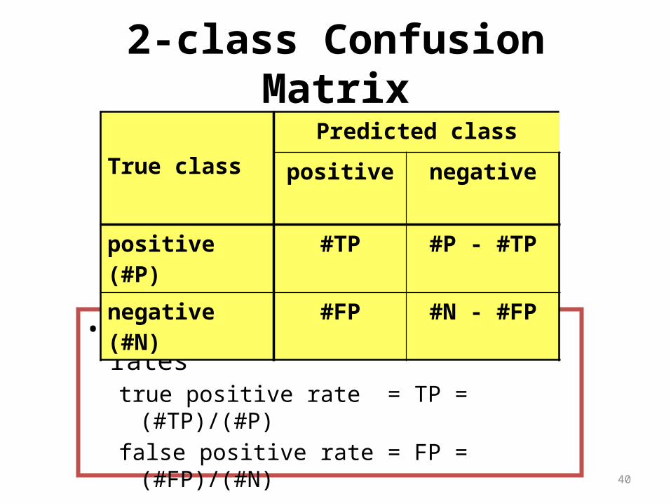
2-class Confusion Matrix
• Reduce the 4 numbers to two ratestrue positive rate = TP = (#TP)/(#P)false positive rate = FP = (#FP)/(#N)
• Rates are independent of class ratio*
True classPredicted class
positive negative
positive (#P) #TP #P - #TP
negative (#N) #FP #N - #FP

41
Example: 3 classifiers
TruePredicted
pos neg
pos 60 40
neg 20 80
TruePredicted
pos neg
pos 70 30
neg 50 50
TruePredicted
pos neg
pos 40 60
neg 30 70
Classifier 1TP = 0.4FP = 0.3
Classifier 2TP = 0.7FP = 0.5
Classifier 3TP = 0.6FP = 0.2
42
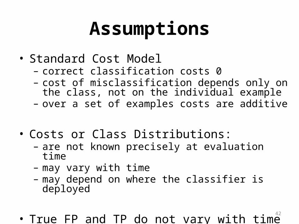
Assumptions• Standard Cost Model
– correct classification costs 0– cost of misclassification depends only on the class, not on
the individual example– over a set of examples costs are additive
• Costs or Class Distributions:– are not known precisely at evaluation time– may vary with time– may depend on where the classifier is deployed
• True FP and TP do not vary with time or location, and are accurately estimated.
43
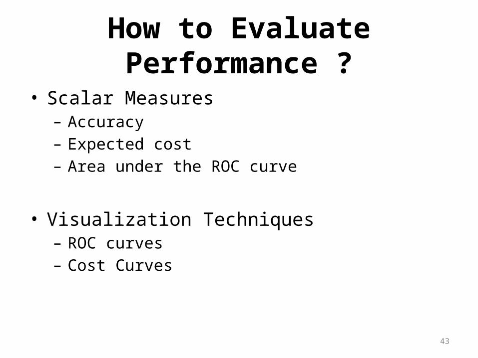
How to Evaluate Performance ?
• Scalar Measures– Accuracy– Expected cost– Area under the ROC curve
• Visualization Techniques– ROC curves– Cost Curves
44
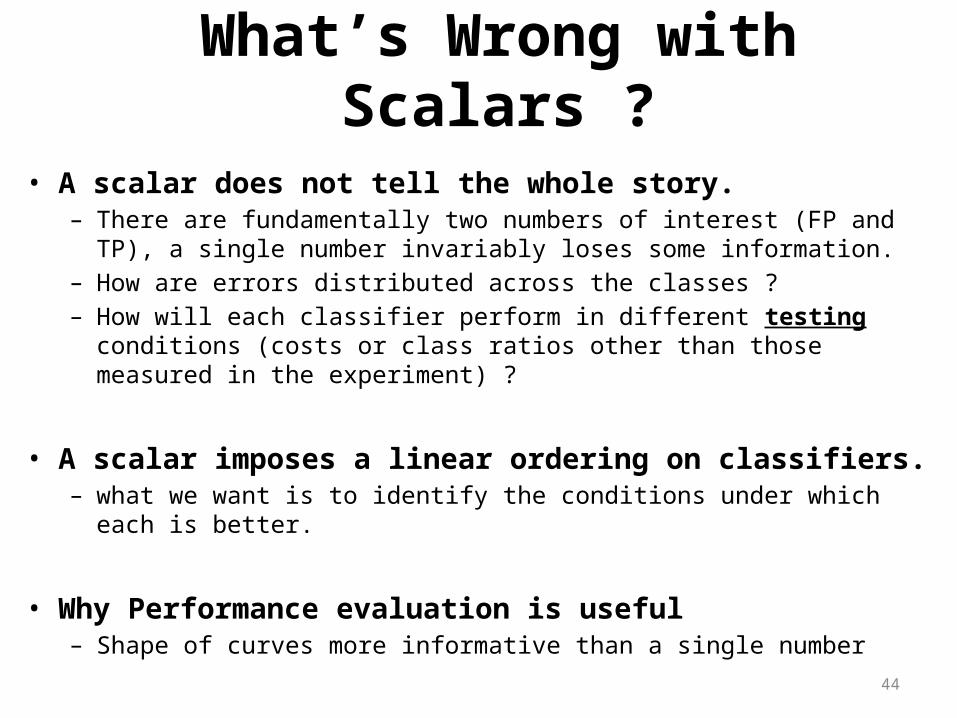
What’s Wrong with Scalars ?
• A scalar does not tell the whole story.– There are fundamentally two numbers of interest (FP and TP), a single
number invariably loses some information.– How are errors distributed across the classes ?– How will each classifier perform in different testing conditions (costs or
class ratios other than those measured in the experiment) ?
• A scalar imposes a linear ordering on classifiers.– what we want is to identify the conditions under which each is better.
• Why Performance evaluation is useful– Shape of curves more informative than a single number
45
ROC Curves
• Receiver operator characteristic
• Summarize & present performance of any binary classification model
• Models ability to distinguish between false & true positives
Receiver Operating Characteristic Curve (ROC)
Analysis• Signal Detection Technique
• Traditionally used to evaluate diagnostic tests
• Now employed to identify subgroups of a population at differential risk for a specific outcome (clinical decline, treatment response)
• Identifies moderators
ROC Analysis: Historical Development (1)
• Derived from early radar in WW2 Battle of Britain to address: Accurately identifying the signals on the radar scan to predict the outcome of interest – Enemy planes – when there were many extraneous signals (e.g. Geese)?
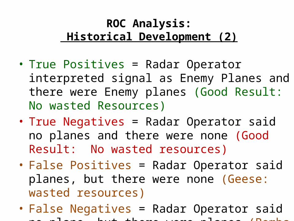
ROC Analysis: Historical Development (2)
• True Positives = Radar Operator interpreted signal as Enemy Planes and there were Enemy planes (Good Result: No wasted Resources)
• True Negatives = Radar Operator said no planes and there were none (Good Result: No wasted resources)
• False Positives = Radar Operator said planes, but there were none (Geese: wasted resources)
• False Negatives = Radar Operator said no plane, but there were planes (Bombs dropped: very bad outcome)
49
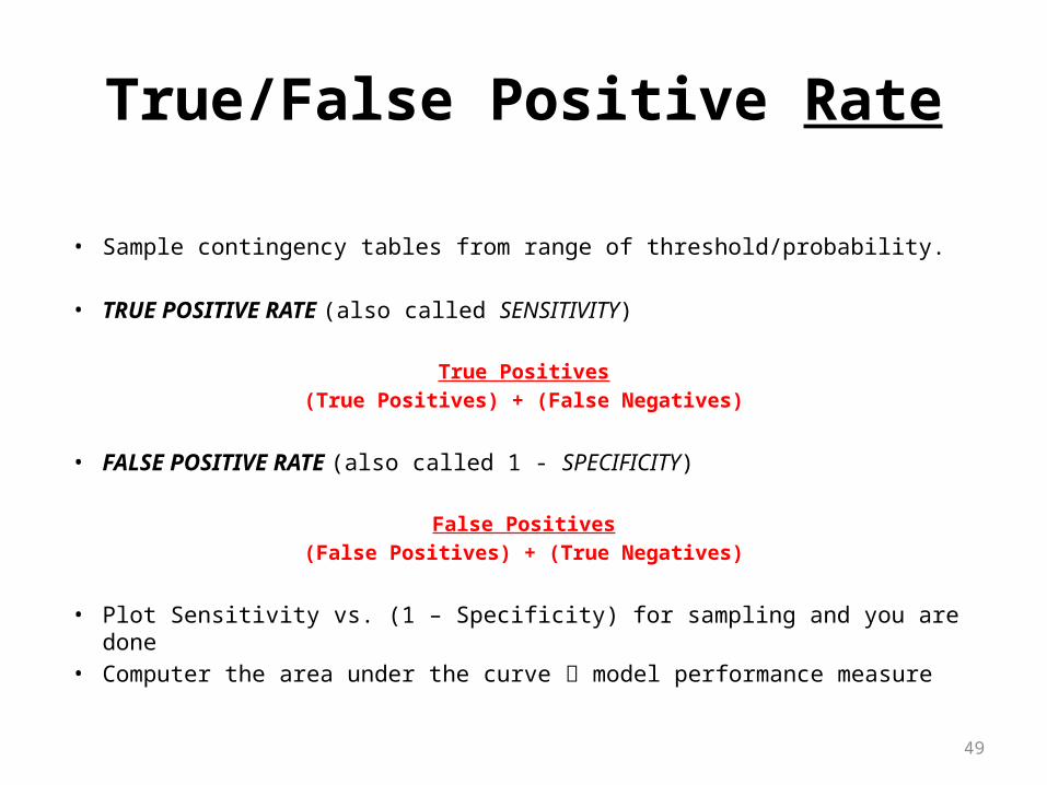
True/False Positive Rate
• Sample contingency tables from range of threshold/probability.
• TRUE POSITIVE RATE (also called SENSITIVITY)
True Positives(True Positives) + (False Negatives)
• FALSE POSITIVE RATE (also called 1 - SPECIFICITY)
False Positives(False Positives) + (True Negatives)
• Plot Sensitivity vs. (1 – Specificity) for sampling and you are done• Computer the area under the curve model performance measure
50
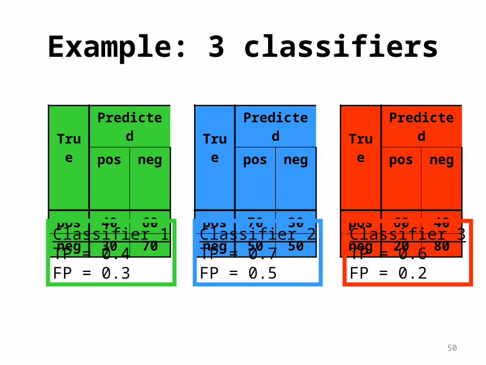
Example: 3 classifiers
TruePredicted
pos neg
pos 60 40
neg 20 80
TruePredicted
pos neg
pos 70 30
neg 50 50
TruePredicted
pos neg
pos 40 60
neg 30 70
Classifier 1TP = 0.4FP = 0.3
Classifier 2TP = 0.7FP = 0.5
Classifier 3TP = 0.6FP = 0.2
51
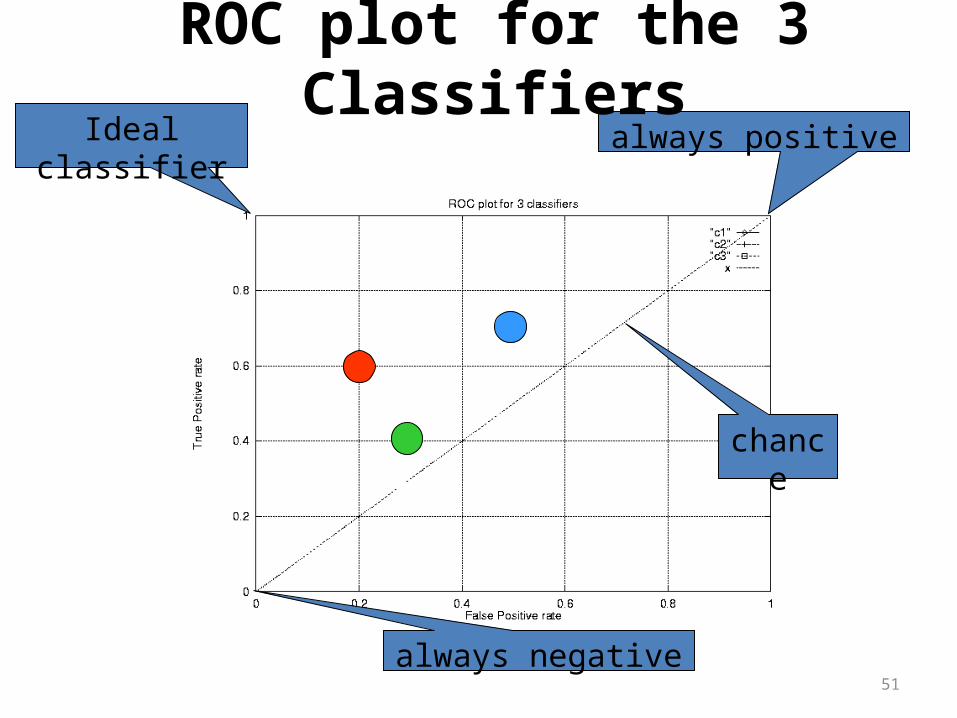
Ideal classifier
chance
always negative
always positive
ROC plot for the 3 Classifiers
52
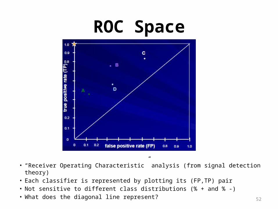
ROC Space
• “Receiver Operating Characteristic” analysis (from signal detection theory)• Each classifier is represented by plotting its (FP,TP) pair• Not sensitive to different class distributions (% + and % -)• What does the diagonal line represent?
53
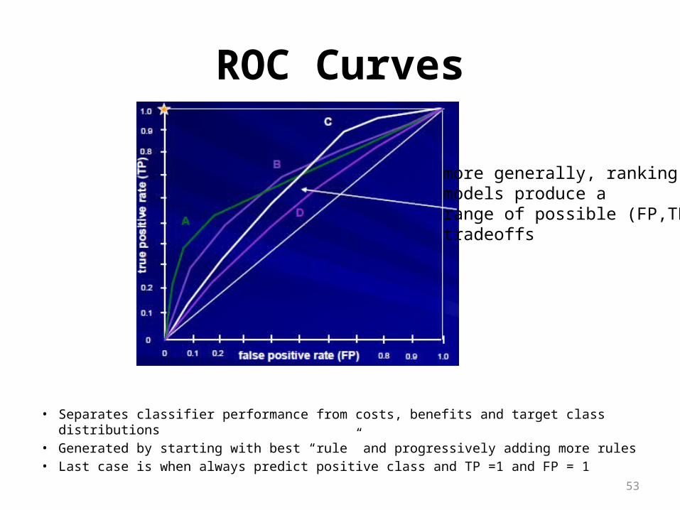
ROC Curves
• Separates classifier performance from costs, benefits and target class distributions• Generated by starting with best “rule” and progressively adding more rules• Last case is when always predict positive class and TP =1 and FP = 1
more generally, rankingmodels produce arange of possible (FP,TP)tradeoffs
54
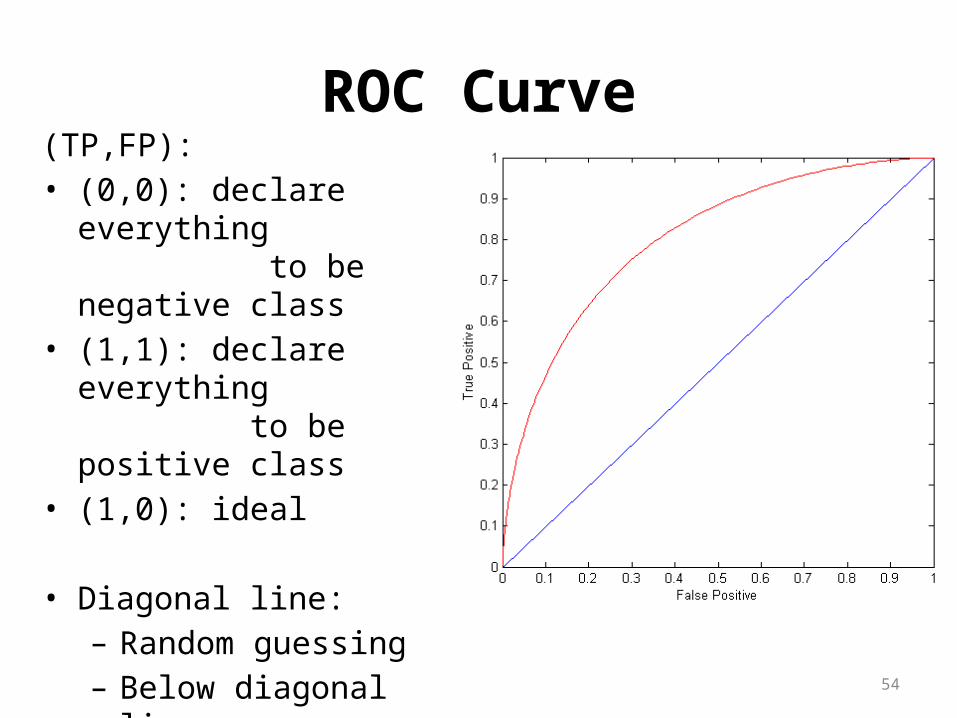
ROC Curve(TP,FP):• (0,0): declare everything
to be negative class• (1,1): declare everything
to be positive class• (1,0): ideal
• Diagonal line:– Random guessing– Below diagonal line:
• prediction is opposite of the true class
55
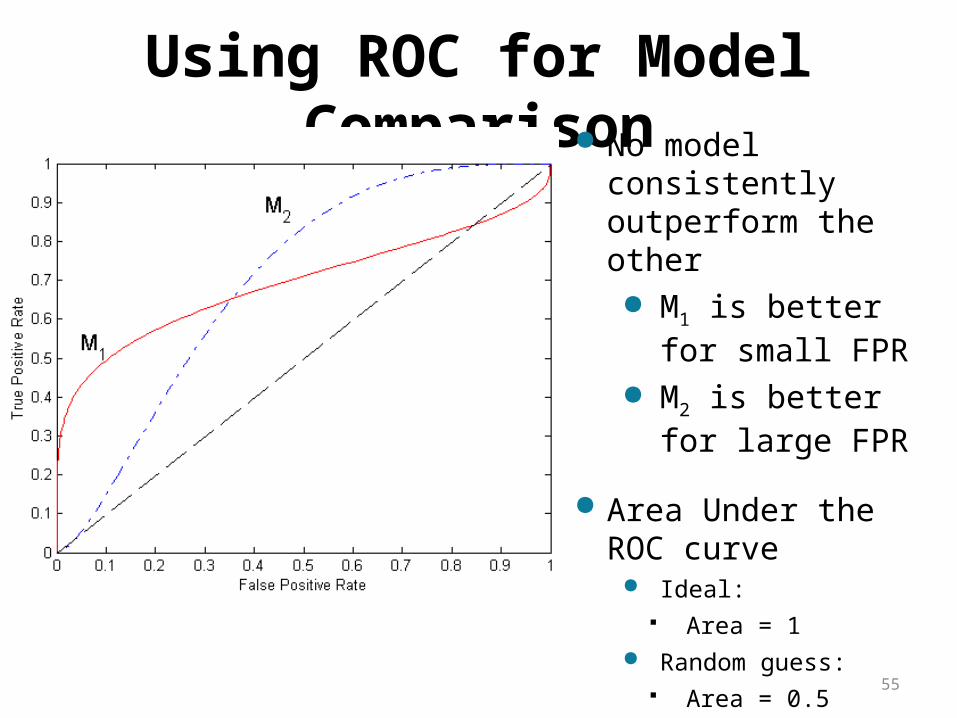
Using ROC for Model Comparison No model consistently
outperform the other M1 is better for small
FPR M2 is better for large
FPR
Area Under the ROC curve
Ideal: Area = 1
Random guess: Area = 0.5
56
Model Evaluation
• Metrics for Performance Evaluation– How to evaluate the performance of a model?
• Methods for Performance Evaluation– How to obtain reliable estimates?
57
Methods for Performance Evaluation
• How to obtain a reliable estimate of performance?
• Performance of a model may depend on other factors besides the learning algorithm:– Class distribution– Cost of misclassification– Size of training and test sets
58
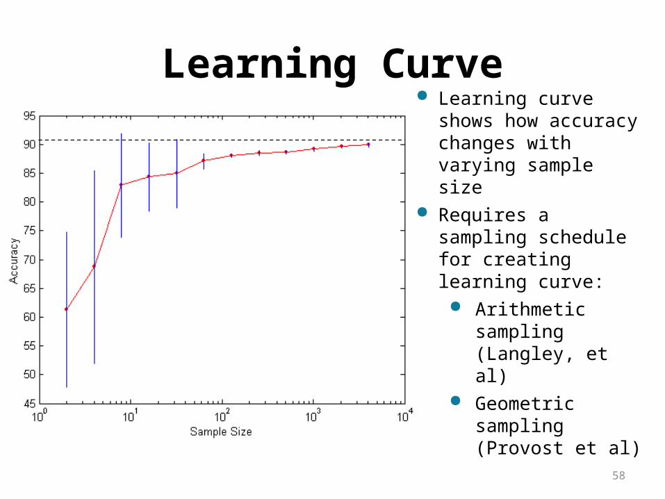
Learning Curve Learning curve shows how
accuracy changes with varying sample size
Requires a sampling schedule for creating learning curve:
Arithmetic sampling(Langley, et al)
Geometric sampling(Provost et al)
59
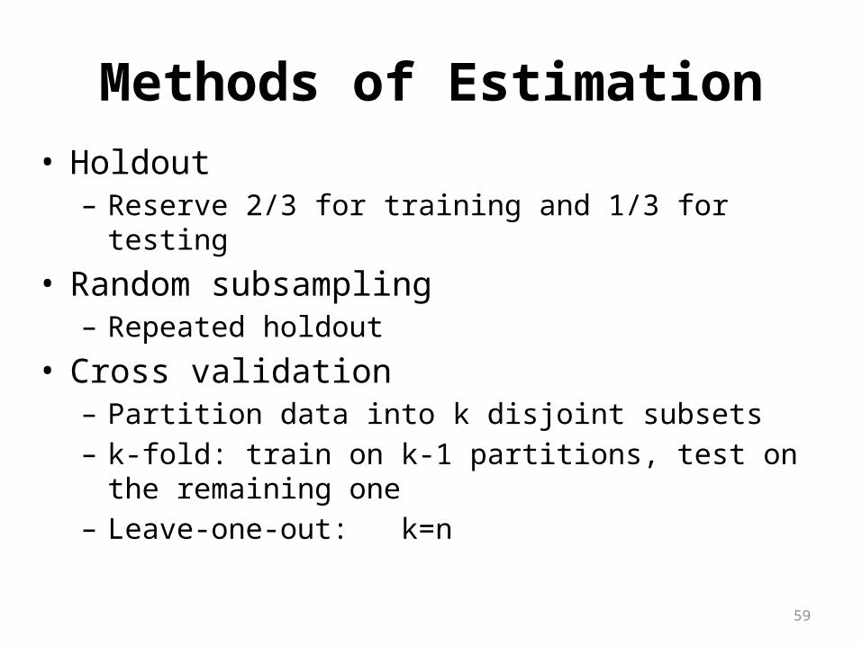
Methods of Estimation• Holdout
– Reserve 2/3 for training and 1/3 for testing
• Random subsampling– Repeated holdout
• Cross validation– Partition data into k disjoint subsets– k-fold: train on k-1 partitions, test on the remaining one– Leave-one-out: k=n
60
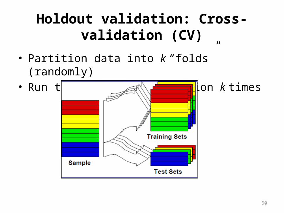
Holdout validation: Cross-validation (CV)
• Partition data into k “folds” (randomly)• Run training/test evaluation k times
61
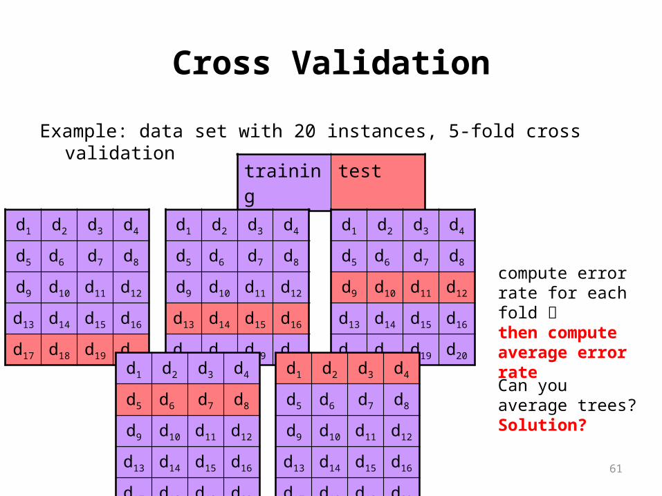
Cross Validation
Example: data set with 20 instances, 5-fold cross validation
training test
d1 d2 d3 d4
d5 d6 d7 d8
d9 d10 d11 d12
d13 d14 d15 d16
d17 d18 d19 d20
d1 d2 d3 d4
d5 d6 d7 d8
d9 d10 d11 d12
d13 d14 d15 d16
d17 d18 d19 d20
d1 d2 d3 d4
d5 d6 d7 d8
d9 d10 d11 d12
d13 d14 d15 d16
d17 d18 d19 d20
d1 d2 d3 d4
d5 d6 d7 d8
d9 d10 d11 d12
d13 d14 d15 d16
d17 d18 d19 d20
d1 d2 d3 d4
d5 d6 d7 d8
d9 d10 d11 d12
d13 d14 d15 d16
d17 d18 d19 d20
compute error rate for each fold then compute average error rate
Can you average trees?Solution?
62
Leave-one-out Cross Validation
• Leave-one-out cross validation is simply k-fold cross validation with k set to n, the number of instances in the data set.
• The test set only consists of a single instance, which will be classified either correctly or incorrectly.
• Advantages: maximal use of training data, i.e., training on n−1 instances. The procedure is deterministic, no sampling involved.
• Disadvantages: unfeasible for large data sets: large number of training runs required, high computational cost.