Embed Size (px)
Citation preview

CLASSIFICATION OF PLANTS USING IMAGES OF THEIR LEAVES
A Thesis by
BIVA SHRESTHA December 2010
APPROVED BY _____________________________________ Rahman Tashakkori Chairperson, Thesis Committee _____________________________________ Alice A. McRae Member, Thesis Committee _____________________________________ Zack E. Murrell Member, Thesis Committee _____________________________________ James T. Wilkes Chairperson, Computer Science _____________________________________ Edelma Huntley Dean, Research and Graduate Studies
CLASSIFICATION OF PLANTS USING IMAGES OF THEIR LEAVES
A Thesis by
BIVA SHRESTHA December 2010
Submitted to the Graduate School Appalachian State University
in partial fulfillment of the requirements for the degree of MASTER OF SCIENCE
December 2010 Major Department: Computer Science

Copyright by Biva Shrestha 2010 All Rights Reserved.
iv
ABSTRACT
CLASSIFICATION OF PLANTS USING IMAGES OF THEIR LEAVES
Biva Shrestha
M.S., Appalachian State University
Thesis Chairperson: Rahman Tashakkori
Plant recognition is a matter of interest for scientists as well as laymen. Computer aided
technologies can make the process of plant recognition much easier; botanists use
morphological features of plants to recognize them. These features can also be used as a
basis for an automated classification tool. For example, images of leaves of different
plants can be studied to determine effective algorithms that could be used in classifying
different plants. In this thesis, those salient features of plant leaves are studied that may
be used as a basis for plant classification and recognition. These features are independent
of leaf maturity and image translation, rotation and scaling and are studied to develop an
approach that produces the best classification algorithm. First, the developed algorithms
are used to classify a training set of images; then, a testing set of images is used for
verifying the classification algorithms.

v
ACKNOWLEDGMENTS
First and foremost, I would like to express my deepest gratitude to my advisor,
Dr. Rahman Tashakkori, for his continuous support and guidance throughout my M.S.
pursuit. His love towards research work and innovation was the biggest motivational
factor for me. He taught me to view a problem as an adventure which has led me to enjoy
my research while meeting the challenges. Without his guidance and persistent help this
thesis would not have been possible.
I would also like to express my heartfelt thanks to my co-advisors, Dr. Alice
McRae and Dr. Zack Murrell, for their valuable advice.
I would like to thank my family for continually believing in me. They have
always encouraged me never to give up in pursuing my goals. Without their love and
presence the successes as well as the failures would have been meaningless.
Finally, I would like to thank my best friend, my guide and my husband, Unnati
Ojha, for always being there for me to discuss and aid me through difficult situations.
Without his help, care and understanding, all of my achievements would have been
unreached.
vi
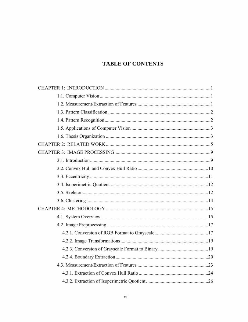
TABLE OF CONTENTS
CHAPTER 1: INTRODUCTION ....................................................................................... 1
1.1. Computer Vision ........................................................................................... 1
1.2. Measurement/Extraction of Features ............................................................ 1
1.3. Pattern Classification .................................................................................... 2
1.4. Pattern Recognition ....................................................................................... 2
1.5. Applications of Computer Vision ................................................................. 3
1.6. Thesis Organization ...................................................................................... 3
CHAPTER 2: RELATED WORK ...................................................................................... 5
CHAPTER 3: IMAGE PROCESSING ............................................................................... 9
3.1. Introduction ................................................................................................... 9
3.2. Convex Hull and Convex Hull Ratio .......................................................... 10
3.3. Eccentricity ................................................................................................. 11
3.4. Isoperimetric Quotient ................................................................................ 12
3.5. Skeleton ....................................................................................................... 12
3.6. Clustering .................................................................................................... 14
CHAPTER 4: METHODOLOGY .................................................................................... 15
4.1. System Overview ........................................................................................ 15
4.2. Image Preprocessing ................................................................................... 17
4.2.1. Conversion of RGB Format to Grayscale ............................................ 17
4.2.2. Image Transformations ........................................................................ 19
4.2.3. Conversion of Grayscale Format to Binary ......................................... 19
4.2.4. Boundary Extraction ............................................................................ 20
4.3. Measurement/Extraction of Features .......................................................... 23
4.3.1. Extraction of Convex Hull Ratio ......................................................... 24
4.3.2. Extraction of Isoperimetric Quotient ................................................... 26
vii
4.3.3. Extraction of Eccentricity .................................................................... 26
4.3.4. Extraction of Aspect Ratio ................................................................... 28
4.3.5. Extraction of Skeleton ......................................................................... 28
4.4. Pattern Classification .................................................................................. 33
4.5. Pattern Recognition ..................................................................................... 36
4.5.1. Training ................................................................................................ 37
4.5.2. Testing ................................................................................................. 38
CHAPTER 5: RESULTS .................................................................................................. 39
5.1. Image Preprocessing ................................................................................... 39
5.2. Convex Hull Ratio ...................................................................................... 41
5.3. Isoperemetric Quotient ................................................................................ 42
5.4. Eccentricity and Aspect Ratio ..................................................................... 42
5.5. Skeleton ....................................................................................................... 43
5.6. Classification ............................................................................................... 48
5.7. Recognition ................................................................................................. 53
CHAPTER 6: Conclusions and Future Recommendations ............................................... 55
6.1. Conclusion .................................................................................................. 55
6.1.1. Isoperemetric Quotient ........................................................................ 55
6.1.2. Eccentricity and Aspect Ratio ............................................................. 56
6.1.3. Convex Hull Ratio ............................................................................... 56
6.1.4. Skeleton ............................................................................................... 56
6.1.5. Summary .............................................................................................. 57
6.2. Future Recommendations ........................................................................... 57
BIBLIOGRAPHY .............................................................................................................. 59
APPENDIX A…. ............................................................................................................... 61
APPENDIX B ……………………………………………………………………………68
APPENDIX C…………………………………………………………………………… 71
VITA…………………………………………………………………………………….. 75

viii
LIST OF TABLES
Table 4-1: Different shapes of leaves used in the classification and their features……...35
Table 5-1: Results of clustering algorithm……………………………………………….53
Table 5-2: Recognition results of the test data set…………………………………….....54
ix
LIST OF FIGURES
Fig. 3.1: Illustration of a convex hull ................................................................................ 10 Fig. 3.2: The best fitting ellipse to a polygon with its major and minor axes ................... 11 Fig. 3.3: a) An arbitrary object, b) and c) various positions of maximum disks with
centers on skeleton of the object, d) the complete skeleton ............................... 13 Fig. 4.1: A sample plant specimen from I. W. Carpenter, Jr. Herbarium .......................... 16 Fig. 4.2: Steps involved in image preprocessing ............................................................... 16 Fig. 4.3: Four steps of methodology .................................................................................. 17 Fig. 4.4: a) An arbitrary RGB image, b) Grayscale equivalent using weighted
averaging, c) Grayscale equivalent using averaging .......................................... 18 Fig. 4.5: A Gaussian filter .................................................................................................. 21 Fig. 4.6: Separation of angles for determining a vertical/horizontal neighbor in non-
maxima suppression ............................................................................................ 23 Fig. 4.7: Feature extraction process ................................................................................... 23 Fig. 4.8: Convex hull by Andrew’s monotone chain algorithm ........................................ 25 Fig. 4.9: Initialization and propagation of U a) a boundary image, b) initialization of
U, c) moving front, and d) assignment of U with the propagating front. ........... 30 Fig. 4.10: a) The maximum distance to the nearest neighbor pixel and b) illustration
of skeletal points. ................................................................................................ 31 Fig. 4.11: Treatment of special boundary points: a) original object, b) initial U, c)
computed U, d) and the extracted skeleton ......................................................... 32 Fig. 4.12: a) An arbitrary triangle, b) its skeleton with green circles as the endpoints
and red circles as the junction points .................................................................. 33 Fig. 4.13: Acicular leaf ...................................................................................................... 35 Fig. 4.14: Orbicular leaf ..................................................................................................... 35 Fig. 4.15: Hastate leaf ........................................................................................................ 35 Fig. 4.16: Elliptical leaf ..................................................................................................... 36 Fig. 4.17: Palmate leaf ....................................................................................................... 36 Fig. 4.18: Lobed leaf .......................................................................................................... 36 Fig. 4.19: Palmate and doubly serrated leaf’s margin ....................................................... 36 Fig. 4.20: Heart shaped leaf ............................................................................................... 36 Fig. 4.21: Margin of a elliptic and serrated leaf ................................................................ 36 Fig. 4.22: The GUI for AppLeClass .................................................................................. 38 Fig. 5.1: a) A hastate leaf in RGB format, b) conversion to grayscale, c) conversion to
binary and d) boundary extraction from the binary image ................................. 39 Fig. 5.2: A leaf with uneven coloring and its boundary detection process ........................ 40 Fig. 5.3: The area bounded by the red polygon represents the convex hull ...................... 41 Fig. 5.4: Convex hull being affected by leaf petiole .......................................................... 41
x
Fig. 5.5: The best fitting ellipse for a) an acicular leaf b) an elliptic leaf c) an orbicular leaf ....................................................................................................... 42
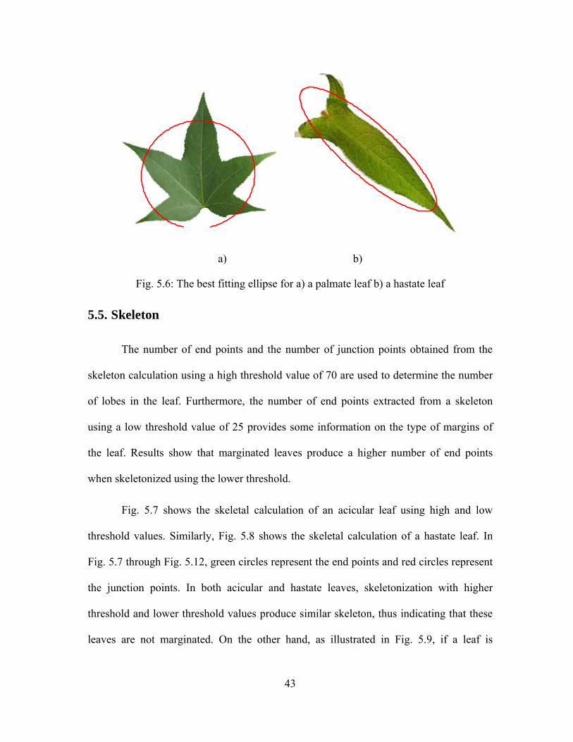
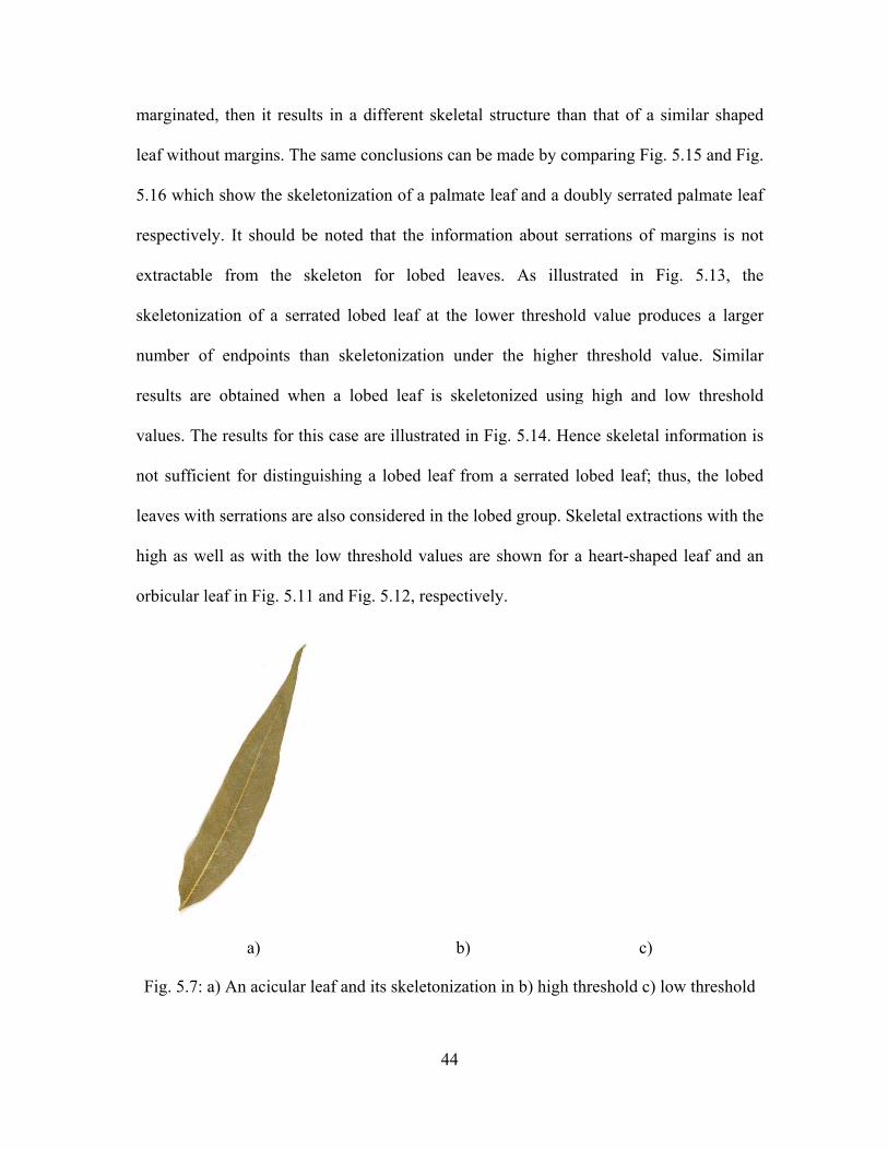
Fig. 5.6: The best fitting ellipse for a) a palmate leaf b) a hastate leaf .............................. 43 Fig. 5.7: a) An acicular leaf and its skeletonization in b) high threshold c) low
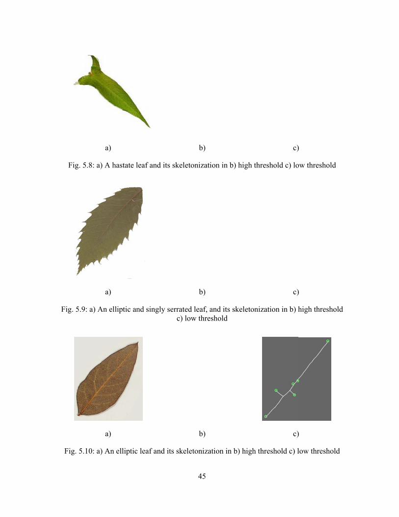
threshold ............................................................................................................. 44 Fig. 5.8: a) A hastate leaf and its skeletonization in b) high threshold c) low threshold ... 45 Fig. 5.9: a) An elliptic and singly serrated leaf, and its skeletonization in b) high
threshold c) low threshold .................................................................................. 45 Fig. 5.10: a) An elliptic leaf and its skeletonization in b) high threshold c) low
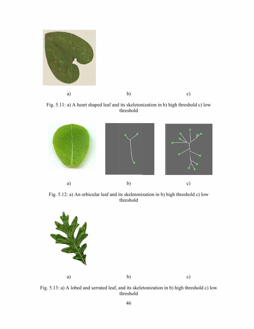
threshold ............................................................................................................. 45 Fig. 5.11: a) A heart shaped leaf and its skeletonization in b) high threshold c) low
threshold ............................................................................................................. 46 Fig. 5.12: a) An orbicular leaf and its skeletonization in b) high threshold c) low
threshold ............................................................................................................. 46 Fig. 5.13: a) A lobed and serrated leaf, and its skeletonization in b) high threshold c)
low threshold ...................................................................................................... 46 Fig. 5.14: a) A lobed leaf and its skeletonization in b) high threshold c) low threshold ... 47 Fig. 5.15: a) A palmate leaf and its skeletonization in b) high threshold c) low
threshold ............................................................................................................. 47 Fig. 5.16: a) A palmate and doubly serrated leaf, and its skeletonization in b) high
threshold c) low threshold .................................................................................. 47 Fig. 5.17: Distribution of isoperimetric quotient ............................................................... 48 Fig. 5.18: Distribution of eccentricity ................................................................................ 49 Fig. 5.19: Distribution of convex hull ratio ....................................................................... 49 Fig. 5.20: Distribution of aspect ratio ................................................................................ 50 Fig. 5.21: Distribution of number of end points estimated from high threshold
skeletonization .................................................................................................... 51 Fig. 5.22: Distribution of number of junction points estimated from high threshold
skeletonization .................................................................................................... 51 Fig. 5.23: Distribution of number of end points estimated from low threshold
skeletonization .................................................................................................... 52
1
CHAPTER 1: INTRODUCTION
1.1. Computer Vision
This thesis focuses on automation through computer vision. Computer vision is
concerned with the theory behind artificial systems that extract information from images.
The image data can take many forms, such as video sequences, views from multiple
cameras, or multi-dimensional data from a medical scanner. In other words, computer
vision is the science and technology of machines that have the ability to see. Snyder [1]
describes the term computer vision as “The process whereby a machine, usually a digital
computer, automatically processes an image and reports ‘what is in the image’, i.e., it
recognizes the content of the image. Often the content may be a machine part, and the
objective is not only to locate the part, but to inspect it as well.” Computer vision, also
known as machine vision, consists of three parts: measurement of features, pattern
classification based on those features, and pattern recognition. This thesis was conducted
to develop a system that extracts different features from a leaf image and classifies
different classes of leaves based on the extracted features. Furthermore, the system uses
the results of the classification scheme in identifying the class of new leaf images.
1.2. Measurement/Extraction of Features
Image processing technologies are used to extract a set of features/measurements
that characterize or represent the image. The values of these features provide a concise
2
representation about the information in the image. For example, a set of features that
characterize a triangle could be the length of each side of the triangle.
1.3. Pattern Classification
Pattern classification is the organization of patterns into groups of patterns sharing
the same set of properties. Given a set of measurements of an unknown object and the
knowledge of possible classes to which an object may belong, a decision about to which
class the unknown object belongs could be made. For example, if information about the
length of sides of an unknown triangle is extracted, a decision on whether the unknown
triangle is an equilateral, isosceles or scalene triangle can be made. Similarly, if a set of
features/measurements is extracted from a leaf, a decision about the possible class of the
leaf can be made. Pattern classification may be statistical or syntactic.
Statistical classification is the classification of individual items into groups based
on quantitative information of one or more features/measurements of the item and based
on a training set of previously classified items. An example of this type of classification
is clustering; this study uses clustering for pattern classification.
Syntactic classification (Structural classification) is the classification of
individual items based on a structure in the pattern of the measurements. Items are
classified syntactically only if there is a clear structure in the pattern of the
measurements.
1.4. Pattern Recognition
Pattern recognition is the process of classifying data or patterns based on the
knowledge/information extracted from patterns. The patterns to be classified are usually
3
groups of measurements or observations defining points in an appropriate
multidimensional space. In this thesis, pattern recognition is implemented on a set of test
images in order to validate and evaluate the performance of the underlying classification
scheme.
1.5. Applications of Computer Vision
Some applications of computer vision are face recognition, fingerprint
recognition, image-based searching, optical character recognition, remote sensing, and
number plate recognition.
This thesis is highly inspired by the real world applications of computer vision.
The key idea of most of these technologies is automation. Automation is an
interdisciplinary concept that uses technologies in the computer world to simplify
complex issues in other disciplines or in everyday life. This research focuses on using
image processing to automate classification and perform plant recognition based on the
images of the leaves. Automatic plant classification and recognition can assist botanists
in their study as well as help laymen in identifying and studying plants. Different shape-
related features were extracted from these images using image processing algorithms.
Depending on these features, a statistical classification of plants was conducted. The
classification scheme was then validated using a set of test images.
1.6. Thesis Organization
This thesis is organized into six chapters: Introduction, Related Work, Image
Processing, Methodology, Results, Conclusions and Future Recommendations. The
Related Work chapter gives a short preview on similar studies that have been done

4
previously and which may be grouped into different categories. The categories are:
extraction of single feature of leaf or flower, leaf image matching of single plant species,
image-based plant recognition, and image-based plant classification. The Methodology
chapter describes different image processing and feature extraction techniques used and
the classification algorithm implemented for correctly identifying the plants based on
their leaves. The Results chapter presents the results of the research and discusses the
significance of extracted features in classifying plants. Finally, the Conclusions and
Future Recommendations chapter summarizes the outcomes of this study, and discusses
possible modifications and improvements.
5
CHAPTER 2: RELATED WORK
Modern plant taxonomy starts with the Linnaeus’ system of classification [2].
This is a plant classification and nomenclature system and is currently used, albeit in a
revised version. In this classification system plants are classified based on their similarity
and dissimilarity. Linnaeus’ classification and nomenclature gives scientific names to
plants and is a universal language for botanists. Classification and nomenclature of plants
is useful only if plants can be recognized. Botanists recognize plants based on their
knowledge and expertise, but for laymen plant recognition is still a complicated task.
Plant recognition can be made simpler by using computer aided automation. A plant
recognition system should be based on a plant classification system because there are
more than one-half million of plants inhabiting the Earth and recognition without
classification is a complex task. Hence, this thesis focuses on an automated plant
classification system.
Studies have been conducted in the past decade on automation of plant
classification and recognition. A handful of these studies were about the extraction of a
single feature from the image of a plant part such as the leaf, or the flower. Some studies
were about the extraction of multiple features but from a single family of plants. Some
studies focused on image-based plant classification, while others focused on image-based
plant recognition. Warren [3] introduced an automatic computerized system that used as
6
its input 10 images of each Chrysanthemum species for testing the variation in the
images. In this study, features such as shape, size and color of the flower, petal, and leaf
were described mathematically. Different rose features were extracted and used in the
recognition scheme for pattern recognition. The study, however, was limited to
Chrysanthemum species only. Miao et al., [4] proposed an evidence-theory-based rose
plant classification using different features of roses. In another study by Heymans et al.,
[5], a back-propagating neural network approach was used to distinguish different leaves
of Opuntia species. Again, the study was limited only to the variety of the Opuntia
family. Saitoh and Kaneko [6] studied an automatic method for recognizing wild flowers.
This recognition required two images: a frontal flower image and a leaf image taken by a
digital camera. Seventeen features, eight from the flower and nine from the leaf, were fed
to a neural network. This research yielded an accuracy of 95% on 20 pairs of pictures
from 16 wild flowers. These studies dealt with a single or group of similar plant species
only.
Some studies focused on extraction of vein features. Li et al., [7] used snake
techniques [8] with cellular neural networks (CNN) to extract the leaf venation feature
from leaf images. Fu and Chi [9] also studied the extraction of leaf venation feature using
neural network. Their methodology involved a preliminary segmentation which is based
on the intensity histogram that coarsely determined the vein regions. This was followed
by segmentation using a trained artificial neural network (ANN) classifier with 10
features extracted from a window centered on pixels within the object. Qi and Yang [10]
studied the extraction of saw tooth feature of the edges of a leaf based on support vector
machine. These studies were limited to the extraction of a single feature only.
7
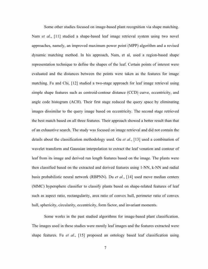
Some other studies focused on image-based plant recognition via shape matching.
Nam et al., [11] studied a shape-based leaf image retrieval system using two novel
approaches, namely, an improved maximum power point (MPP) algorithm and a revised
dynamic matching method. In his approach, Nam, et al, used a region-based shape
representation technique to define the shapes of the leaf. Certain points of interest were
evaluated and the distances between the points were taken as the features for image
matching. Fu and Chi, [12] studied a two-stage approach for leaf image retrieval using
simple shape features such as centroid-contour distance (CCD) curve, eccentricity, and
angle code histogram (ACH). Their first stage reduced the query space by eliminating
images dissimilar to the query image based on eccentricity. The second stage retrieved
the best match based on all three features. Their approach showed a better result than that
of an exhaustive search. The study was focused on image retrieval and did not contain the
details about the classification methodology used. Gu et al., [13] used a combination of
wavelet transform and Gaussian interpolation to extract the leaf venation and contour of
leaf from its image and derived run length features based on the image. The plants were
then classified based on the extracted and derived features using 1-NN, k-NN and radial
basis probabilistic neural network (RBPNN). Du et al., [14] used move median centers
(MMC) hypersphere classifier to classify plants based on shape-related features of leaf
such as aspect ratio, rectangularity, area ratio of convex hull, perimeter ratio of convex
hull, sphericity, circularity, eccentricity, form factor, and invariant moments.
Some works in the past studied algorithms for image-based plant classification.
The images used in these studies were mostly leaf images and the features extracted were
shape features. Fu et al., [15] proposed an ontology based leaf classification using
8
information from leaf images. Their ontology had two main branches, namely, shape and
venation. Shape was classified according to lobation and margin. Lobation and margin
had further sub branches describing the structure of lobe or margin. Their study, however,
did not reveal the number of test cases used and its overall success rate. Wang et al., [16]
used a MMC hypersphere classifier for classifying plants based on certain leaf features.
First, image segmentation was applied to the leaf images; then eight geometric features
such as rectangularity, circularity, eccentricity, and seven moment invariants were
extracted for classification. Finally, a hypersphere classifier was used to address these
shape features. Wu et al., [17] used a probabilistic neural network for classification of
leaf images based on 12 leaf features. A principal component analysis (PCA) was used
for reducing the 12 dimensions into five dimensions for faster processing. The 12 features
used were physiological length, physiological width, leaf area, leaf perimeter, smooth
factor, aspect ratio, form factor, rectangularity, narrow factor, perimeter ratio of diameter,
perimeter ratio of physiological length and physiological width, and vein features. The
use of scale variant features such as physiological length, physiological width, area, and
perimeter might constrain this approach into using standard size for the leaf image. If a
standard size image is not used then the features of the same leaf vary with different sizes
images. Since it is the same leaf, the value of all the features are expected to be same.
The values for these features vary for different scaled versions of the same leaf image. In
this research features used are scaling, translation and rotation invariant. In addition, a
distinct shape feature, skeleton, is introduced for classification of leaves.
9
CHAPTER 3: IMAGE PROCESSING
3.1. Introduction
An image can be defined as a two-dimensional function, ( , ),f x y where x and y
are spatial coordinates, and f is the amplitude at any pair of coordinates ( , )x y [1]. A
digital image is a two-dimensional matrix with discrete value for position as well as
intensity. Pixels represent the position and the value of the pixel represents the intensity
at that position. A binary image is an image with only two intensity values, zero or one. A
grayscale image is an image whose intensities are a range of values representing different
levels of gray. There are various formats of a colored image. In red-green-blue (RGB)
format, the intensity at each pixel is represented by a vector that contains the blue, red
and green levels.
Digital image processing refers to the processing of digital images by means of a
computer. There is a vast range of applications of digital image processing; two examples
are X-ray imaging and Gamma-ray imaging. Digital image processing is also used as a
basis for image-based automatic systems such as automatic face recognition, fingerprint
recognition, etc. This thesis focuses on using digital image processing for the purpose of
automation. Digital images of plant leaves are processed using various algorithms to
extract shape related features. Finally, the classification is done based on the extracted
10
features. Some terminologies that address various features are explained in Sec. 3.2
through Sec. 3.6.
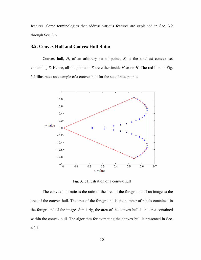
3.2. Convex Hull and Convex Hull Ratio
Convex hull, H, of an arbitrary set of points, S, is the smallest convex set
containing S. Hence, all the points in S are either inside H or on H. The red line on Fig.
3.1 illustrates an example of a convex hull for the set of blue points.
Fig. 3.1: Illustration of a convex hull
The convex hull ratio is the ratio of the area of the foreground of an image to the
area of the convex hull. The area of the foreground is the number of pixels contained in
the foreground of the image. Similarly, the area of the convex hull is the area contained
within the convex hull. The algorithm for extracting the convex hull is presented in Sec.
4.3.1.
11
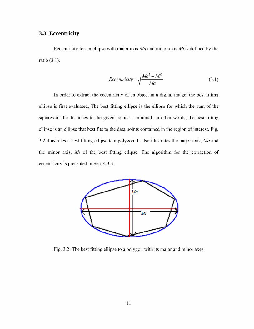
3.3. Eccentricity
Eccentricity for an ellipse with major axis Ma and minor axis Mi is defined by the
ratio (3.1).
2 2Ma MiEccentricityMa−
= (3.1)
In order to extract the eccentricity of an object in a digital image, the best fitting
ellipse is first evaluated. The best fitting ellipse is the ellipse for which the sum of the
squares of the distances to the given points is minimal. In other words, the best fitting
ellipse is an ellipse that best fits to the data points contained in the region of interest. Fig.
3.2 illustrates a best fitting ellipse to a polygon. It also illustrates the major axis, Ma and
the minor axis, Mi of the best fitting ellipse. The algorithm for the extraction of
eccentricity is presented in Sec. 4.3.3.
Fig. 3.2: The best fitting ellipse to a polygon with its major and minor axes
12
3.4. Isoperimetric Quotient
Denoting P as the perimeter of the foreground of an image and A as the area of
the foreground, the isoperimetric quotient is given by (3.2). The algorithm for extraction
of isoperimetric quotient is discussed in Sec. 4.3.2.
2
4 AIsoperemetric quoitentPπ
= (3.2)
3.5. Skeleton
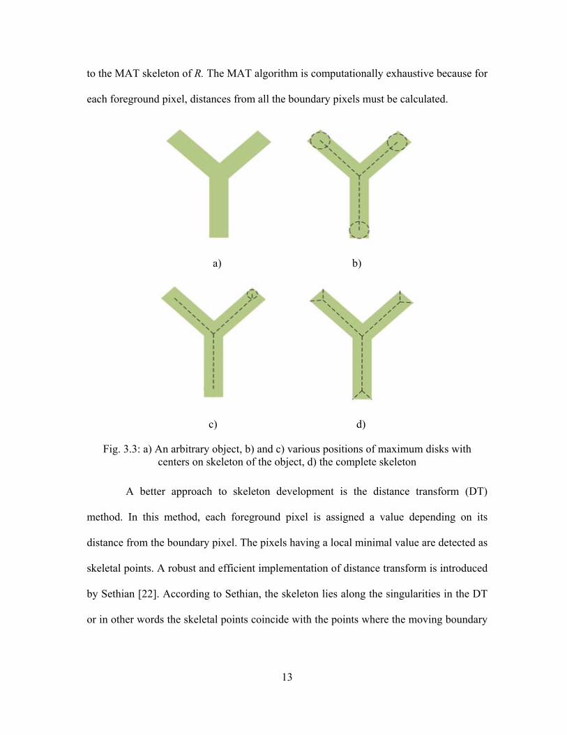
According to Talea [18] the skeleton of a shape is a compact representation of 2D
or 3D such that it preserves many of the topological and size characteristics.
Mathematically, the skeleton is the locus of centers of the maximum disk contained in the
original object [19]-[20]. As illustrated in Fig. 3.3, the line joining the centers of all the
disks touching at least two boundary points of the shape gives the skeleton of the shape.
Talea proposes three methods for the calculation of skeleton:
• Morphological Method
• Geometric Method
• Distance Transform
The morphological method, also known as morphological thinning, iteratively
peels off the boundary layer, identifying points whose removal does not affect the
object’s topology. This method has the disadvantage of missing connectivity.
The geometric method proposed by Ogniewicz [21] is a medial axis transform
(MAT) algorithm. For each point p in an arbitrary region R, its closest neighbor in the
boundary of R, is found and if p has more than one such neighbor, then p is said to belong
13
to the MAT skeleton of R. The MAT algorithm is computationally exhaustive because for
each foreground pixel, distances from all the boundary pixels must be calculated.
a) b)
c) d)
Fig. 3.3: a) An arbitrary object, b) and c) various positions of maximum disks with centers on skeleton of the object, d) the complete skeleton
A better approach to skeleton development is the distance transform (DT)
method. In this method, each foreground pixel is assigned a value depending on its
distance from the boundary pixel. The pixels having a local minimal value are detected as
skeletal points. A robust and efficient implementation of distance transform is introduced
by Sethian [22]. According to Sethian, the skeleton lies along the singularities in the DT
or in other words the skeletal points coincide with the points where the moving boundary
14
collapses onto itself. This thesis uses an augmented fast-marching method proposed by
Talea [18] for the calculation of the skeleton. The algorithm is described in Chap. 4.
3.6. Clustering
Clustering or cluster analysis is a classification method by which a set of data
points or observations are classified into subsets or clusters such that similar data points
lie in the same cluster. It is a common technique for statistical data analysis and is used in
machine vision and image analysis. One of the clustering techniques, K-means clustering,
is used in this thesis for the purpose of leaf image classification. K-means clustering is an
algorithm to classify the objects based on attributes/features into K number of groups
where K is a positive integer. The grouping is done by minimizing the sum of squares of
distances between data and the corresponding cluster centroid. K-means clustering is a
supervised learning algorithm and requires a prior knowledge of the number of clusters.
15
CHAPTER 4: METHODOLOGY
4.1. System Overview
The primary source of leaf images is the Irvin Watson Carpenter, Jr. Herbarium
located in the Department of Biology at Appalachian State University. Images are also
taken from the Robert K. Godfrey Herbarium at Florida State University, and the
University of North Carolina Herbarium. These herbaria have databases of specimens,
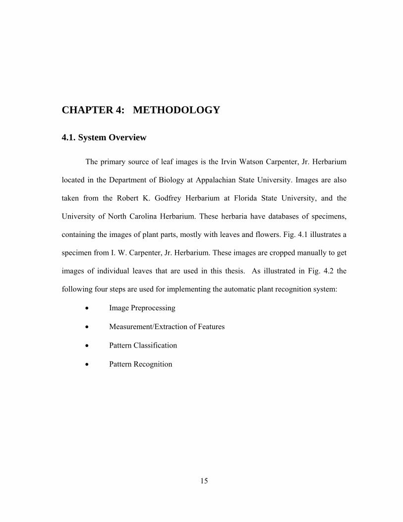
containing the images of plant parts, mostly with leaves and flowers. Fig. 4.1 illustrates a
specimen from I. W. Carpenter, Jr. Herbarium. These images are cropped manually to get
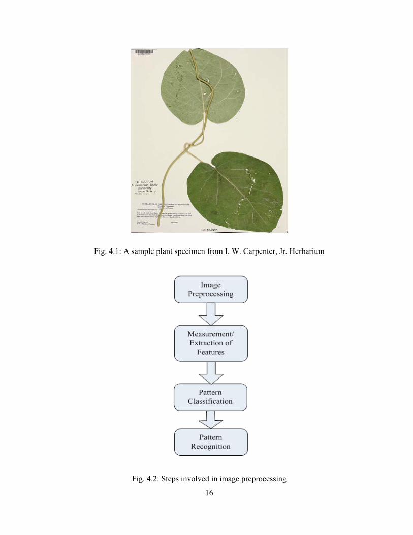
images of individual leaves that are used in this thesis. As illustrated in Fig. 4.2 the
following four steps are used for implementing the automatic plant recognition system:
• Image Preprocessing
• Measurement/Extraction of Features
• Pattern Classification
• Pattern Recognition
16
Fig. 4.1: A sample plant specimen from I. W. Carpenter, Jr. Herbarium
Fig. 4.2: Steps involved in image preprocessing
17
4.2. Image Preprocessing
The images acquired from the Irvin Watson Carpenter, Jr. Herbarium are not
suitable for image processing because they are a large size (up to 17 Megabytes) and they
are RGB images. It is computationally expensive to process a 17 Megabytes, colored
image. Extraction of features is simpler with binary images because all the pixel values in
a binary image can either be zero or one, hence, computations become simpler. Thus, the
images are preprocessed and converted into smaller size files in binary format without the
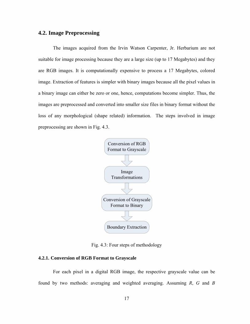
loss of any morphological (shape related) information. The steps involved in image
preprocessing are shown in Fig. 4.3.
Fig. 4.3: Four steps of methodology
4.2.1. Conversion of RGB Format to Grayscale
For each pixel in a digital RGB image, the respective grayscale value can be
found by two methods: averaging and weighted averaging. Assuming R, G and B
Conversion of RGB Format to Grayscale
Image Transformations
Conversion of Grayscale Format to Binary
Boundary Extraction
18
represent the respective intensities for red, green and blue channel of a pixel, then the
averaging algorithm would calculate the respective grayscale intensity, GI using (4.1).
3
R G BGI + += (4.1)
The weighted averaging method is similar to the averaging method except that
some weighting factor is given to each of the color intensities. The weights used in this
research are defined in (4.2).
0.2989 0.5870 0.1140GI R G B= ∗ + ∗ + ∗ (4.2)
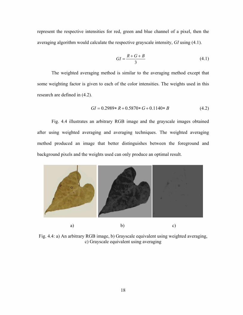
Fig. 4.4 illustrates an arbitrary RGB image and the grayscale images obtained
after using weighted averaging and averaging techniques. The weighted averaging
method produced an image that better distinguishes between the foreground and
background pixels and the weights used can only produce an optimal result.
a) b) c)
Fig. 4.4: a) An arbitrary RGB image, b) Grayscale equivalent using weighted averaging, c) Grayscale equivalent using averaging
19
4.2.2. Image Transformations
The transformation of coordinates or pixels in an image by performing operations
such as scaling, rotation, translation, and shear can be expressed in a general form as
shown in (4.3)
1 1
x vy T w⎡ ⎤ ⎡ ⎤⎢ ⎥ ⎢ ⎥=⎢ ⎥ ⎢ ⎥⎢ ⎥ ⎢ ⎥⎣ ⎦ ⎣ ⎦
(4.3)
where, (v, w) is pixel in the original image, (x, y) is the corresponding pixel coordinate in
the transformed image and T is the transformation matrix. In this thesis scaling
transformation is used to reduce the size of the image file. An example of scaling is
reducing the image size by half, which is shown in (4.4)
1 0 02
10 02
1 10 0 1
x vy w
⎡ ⎤⎢ ⎥
⎡ ⎤ ⎡ ⎤⎢ ⎥⎢ ⎥ ⎢ ⎥⎢ ⎥=⎢ ⎥ ⎢ ⎥⎢ ⎥⎢ ⎥ ⎢ ⎥⎢ ⎥⎣ ⎦ ⎣ ⎦
⎢ ⎥⎢ ⎥⎣ ⎦
(4.4)
In this research, the inverse mapping algorithm is used for image resizing. The
output pixel at each location, (x, y), is computed as an accumulated contribution of
relevant input pixels which are the neighboring pixels. The output pixel value is
determined by interpolating between the nearest input pixels.
4.2.3. Conversion of Grayscale Format to Binary
Once a grayscale image of reduced size is obtained, it is converted to binary
format. To convert a grayscale image into a binary image, Otsu’s [23] method of
automatic thresholding is used. During the thresholding process, pixels in an image are
20
marked as foreground if their values are larger than some threshold and as background
otherwise. The shape of the histogram is used for automatic thresholding and the
threshold is chosen so as to minimize the interclass variance of the black and white
pixels.
4.2.4. Boundary Extraction
The Canny edge detector is used for edge detection and extraction of the region of
interest. The Canny edge detection algorithm consists of four basic steps:
• smoothing the input image with a Gaussian filter
• computing the gradient magnitude and angle images.
• using double thresholding and connectivity analysis to detect and link
edges.
• applying non-maxima suppression to the gradient magnitude image.
Step 1: Smoothing the input image with Gaussian filter
A 2-D Gaussian function, G, expressed by (4.5) is used for image smoothing.
( )2 2
222
1,2
x yaG x y e+
−=
πσ (4.5)
where, a > 0, is a constant, σ is Euler’s constant, and ( ),f x y denotes the input image. If
G(a, b) denotes a discrete Gaussian filter of size m by n, the smoothened image, fs(i, j) is
formed by convolving G and f and the intensity value at pixel (i, j) is given by (4.6).
1 1
( , ) ( , ) ( , )m n
sa b
f i j f i a j b G a b= =
= − −∑∑ (4.6)
A Gaussian filter has an impulse response of Gaussian nature.
21
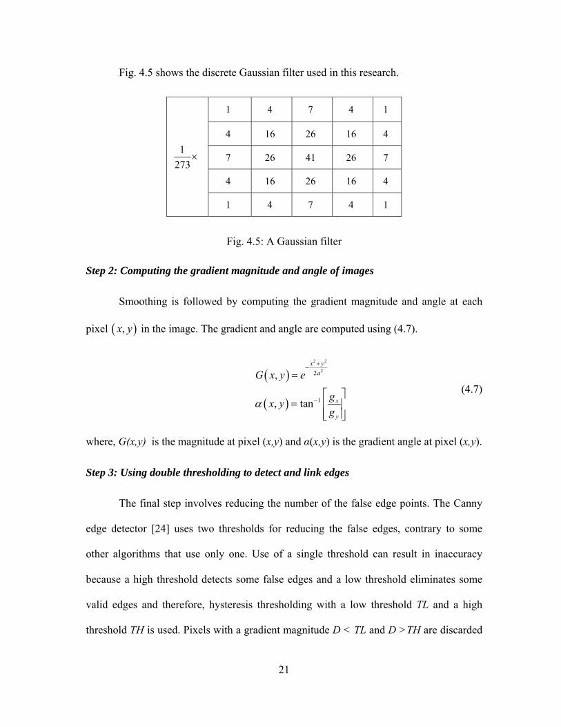
Fig. 4.5 shows the discrete Gaussian filter used in this research.
1273
×
1 4 7 4 1
4 16 26 16 4
7 26 41 26 7
4 16 26 16 4
1 4 7 4 1
Fig. 4.5: A Gaussian filter
Step 2: Computing the gradient magnitude and angle of images
Smoothing is followed by computing the gradient magnitude and angle at each
pixel ( ),x y in the image. The gradient and angle are computed using (4.7).
( )
( )
2 2
22
1
,
, tan
x ya
x
y
G x y e
gx yg
α
+−
−
=
⎡ ⎤= ⎢ ⎥
⎢ ⎥⎣ ⎦
(4.7)
where, G(x,y) is the magnitude at pixel (x,y) and α(x,y) is the gradient angle at pixel (x,y).
Step 3: Using double thresholding to detect and link edges
The final step involves reducing the number of the false edge points. The Canny
edge detector [24] uses two thresholds for reducing the false edges, contrary to some
other algorithms that use only one. Use of a single threshold can result in inaccuracy
because a high threshold detects some false edges and a low threshold eliminates some
valid edges and therefore, hysteresis thresholding with a low threshold TL and a high
threshold TH is used. Pixels with a gradient magnitude D < TL and D >TH are discarded
22
immediately; however, pixels with a magnitude D, such that TL ≤D < TH, are kept
intact.
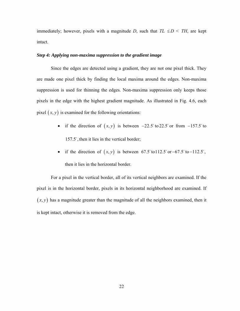
Step 4: Applying non-maxima suppression to the gradient image
Since the edges are detected using a gradient, they are not one pixel thick. They
are made one pixel thick by finding the local maxima around the edges. Non-maxima
suppression is used for thinning the edges. Non-maxima suppression only keeps those
pixels in the edge with the highest gradient magnitude. As illustrated in Fig. 4.6, each
pixel ( ),x y is examined for the following orientations:
• if the direction of ( ),x y is between 22.5− o to 22.5o or from 157.5− o to
157.5 ,o then it lies in the vertical border;
• if the direction of ( ),x y is between 67.5o to112.5o or 67.5− o to 112.5 ,− o
then it lies in the horizontal border.
For a pixel in the vertical border, all of its vertical neighbors are examined. If the
pixel is in the horizontal border, pixels in its horizontal neighborhood are examined. If
( ),x y has a magnitude greater than the magnitude of all the neighbors examined, then it
is kept intact, otherwise it is removed from the edge.
23
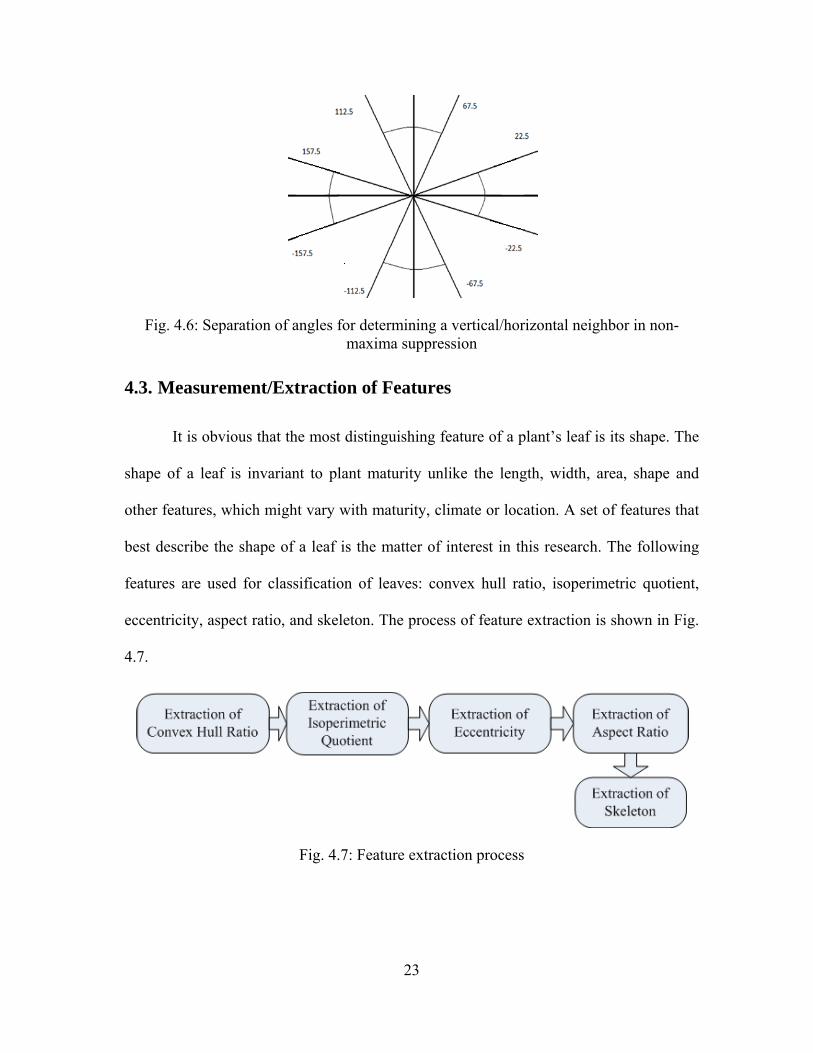
Fig. 4.6: Separation of angles for determining a vertical/horizontal neighbor in non-maxima suppression
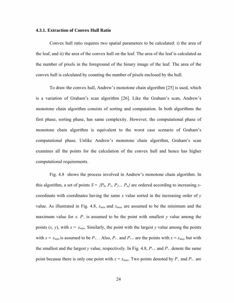
4.3. Measurement/Extraction of Features
It is obvious that the most distinguishing feature of a plant’s leaf is its shape. The
shape of a leaf is invariant to plant maturity unlike the length, width, area, shape and
other features, which might vary with maturity, climate or location. A set of features that
best describe the shape of a leaf is the matter of interest in this research. The following
features are used for classification of leaves: convex hull ratio, isoperimetric quotient,
eccentricity, aspect ratio, and skeleton. The process of feature extraction is shown in Fig.
4.7.
Fig. 4.7: Feature extraction process
24
4.3.1. Extraction of Convex Hull Ratio
Convex hull ratio requires two spatial parameters to be calculated: i) the area of
the leaf, and ii) the area of the convex hull on the leaf. The area of the leaf is calculated as
the number of pixels in the foreground of the binary image of the leaf. The area of the
convex hull is calculated by counting the number of pixels enclosed by the hull.
To draw the convex hull, Andrew’s monotone chain algorithm [25] is used, which
is a variation of Graham’s scan algorithm [26]. Like the Graham’s scan, Andrew’s
monotone chain algorithm consists of sorting and computation. In both algorithms the
first phase, sorting phase, has same complexity. However, the computational phase of
monotone chain algorithm is equivalent to the worst case scenario of Graham’s
computational phase. Unlike Andrew’s monotone chain algorithm, Graham’s scan
examines all the points for the calculation of the convex hull and hence has higher
computational requirements.
Fig. 4.8 shows the process involved in Andrew’s monotone chain algorithm. In
this algorithm, a set of points S = P0, P1, P2… Pn are ordered according to increasing x-
coordinate with coordinates having the same x value sorted in the increasing order of y
value. As illustrated in Fig. 4.8, xmin and xmax are assumed to be the minimum and the
maximum value for x. P-- is assumed to be the point with smallest y value among the
points (x, y), with x = xmin. Similarly, the point with the largest y value among the points
with x = xmin is assumed to be P+- . Also, P+- and P++ are the points with x = xmax but with
the smallest and the largest y value, respectively. In Fig. 4.8, P++ and P+- denote the same
point because there is only one point with x = xmax. Two points denoted by P-- and P+- are
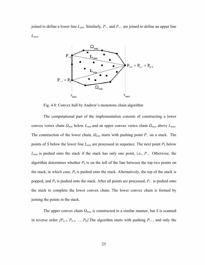
25
joined to define a lower line Lmin. Similarly, P-+ and P++ are joined to define an upper line
Lmax.
Fig. 4.8: Convex hull by Andrew’s monotone chain algorithm
The computational part of the implementation consists of constructing a lower
convex vertex chain Ωmin below Lmin and an upper convex vertex chain Ωmax above Lmax.
The construction of the lower chain, Ωmin starts with pushing point P-- on a stack. The
points of S below the lower line Lmin are processed in sequence. The next point Pk below
Lmin is pushed onto the stack if the stack has only one point, i.e., P--. Otherwise, the
algorithm determines whether Pk is on the left of the line between the top two points on
the stack, in which case, Pk is pushed onto the stack. Alternatively, the top of the stack is
popped, and Pk is pushed onto the stack. After all points are processed, P+- is pushed onto
the stack to complete the lower convex chain. The lower convex chain is formed by
joining the points in the stack.
The upper convex chain Ωmax is constructed in a similar manner, but S is scanned
in reverse order Pn-1, Pn-2, ..., P0.The algorithm starts with pushing P++, and only the
26
points above Lmax are scanned. Once the two hull chains are determined, they are joined
to form the complete convex hull.
4.3.2. Extraction of Isoperimetric Quotient
Extraction of the isoperimetric quotient required extraction of the area and the
perimeter of leaves. Given a binary leaf image, the area is calculated as the number of
pixels in the foreground. Canny edge detector is used to get the edge image for the
foreground region and perimeter is calculated as the number of pixels in the boundary of
the foreground region.
4.3.3. Extraction of Eccentricity
For the extraction of eccentricity, the best fitting ellipse is first estimated using a
region-based method. Unlike a boundary-based method, which uses boundary
information to find the best fit, this region-based method uses the moments of a shape to
estimate the best fitting ellipse. Region-based methods are faster because they are not
affected by the irregularities of the shape.
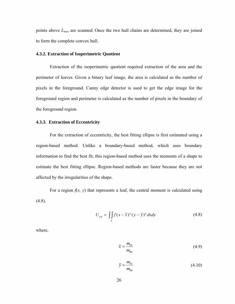
For a region f(x, y) that represents a leaf, the central moment is calculated using
(4.8).
( ) ( )p qpq
g
U f x x y y dxdy= − −∫ ∫ (4.8)
where,
10
00
mxm
= (4.9)
01
00
mym
= (4.10)
27
and ( , )x y represents the centroid of the region f. (m10,m01) is the sum of x-coordinates
and y-coordinates of points in the foreground and m00 is the area of f. The first six central
moments are expressed as shown in (4.11) through (4.15).
00 00u m= (4.11)
10 01 0u u= = (4.12)
210
20 2000
mu mm
= − (4.13)
2
0102 02
00
mu mm
= − (4.14)
10 0111 11
00
m mu mm
= − (4.15)
The normalized central moments are defined using (4.16).
00
pqpq
un
uγ= (4.16)
where,
12
p qγ += + (4.17)
The central moments are used to define the best fit ellipse. For an arbitrary shape
oriented at an angle Ø, with minor axis, a, and major axis, b, the values for these three
parameters are calculated using (4.18), (4.19) and (4.20), respectively.
0 02
11
2( )u uau+ + Δ
= (4.18)
20 02
11
2( )u ubu+ − Δ
= (4.19)
28
1 11
20 02
21 tan2
uu u
φ − ⎛ ⎞= ⎜ ⎟−⎝ ⎠
(4.20)
where,
( )2211 20 024u u uΔ = + − (4.21)
4.3.4. Extraction of Aspect Ratio
For a rectangular shape, aspect ratio is the ratio of its breadth by length. Since
leaves have irregular shapes, their aspect ratio is defined as the ratio of the minor axis to
the major axis of the best fitting ellipse.
4.3.5. Extraction of Skeleton
The skeleton of a leaf is extracted using the augmented fast marching method
(AFMM) [18]. AFMM is based on the observation that skeletal points are always
generated by compact boundary points that collapse as the moving fronts advance inward
starting across the boundary. As the name suggests, augmented fast marching is a
development in the fast marching method [22]. For extraction of the skeleton, each pixel
(i, j) in the boundary is assigned a flag value f according to the rules given below:
• f(i, j) = BAND, if the pixel belongs to the current position of the moving font.
• f(i, j) = INSIDE, if the pixel is inside the moving font.
• f(i, j) = KNOWN, if the pixel value is outside the moving font.
29
Each pixel (i, j) in the foreground is assigned a U value. With the above
assumptions the following four steps of AFMM are used: initialization, propagation,
thresholding, and special boundary points’ detection.
Step 1: Initialization
An arbitrary boundary point P, is assigned a value U = 0. Starting at P the U value
is incremented monotonically along the boundary as illustrated in Fig. 4.9 b). All the
boundary pixels are assigned f(i, j) = KNOWN since their U value is known. The pixels
inside the boundary are assigned f(i, j) = INSIDE and the pixels outside the boundary are
assigned f(i, j) = KNOWN.
Step 2: Propagation
Assuming (k, l) is a pixel with known U value, each pixel (i, j) next to the
neighbor (k, l) is assigned the value of U using the following algorithm:
If f(i, j) = INSIDE f(i, j) = BAND;
a = average of U over KNOWN neighbors of (i, j);
m = min of U over KNOWN neighbors of (i, j)
M = max of U over KNOWN neighbors of (i, j)
If ((M - m) < 2) U(i, j) = a;
else U(i, j) = U(k, l);
The evaluation of f(i, j) during propagation is done the same way as in
initialization. Fig. 4.9 a) and b) illustrate the initialization of U for a continuous
foreground. Similarly, Fig. 4.9 c) and d) illustrate the initialization of U for a
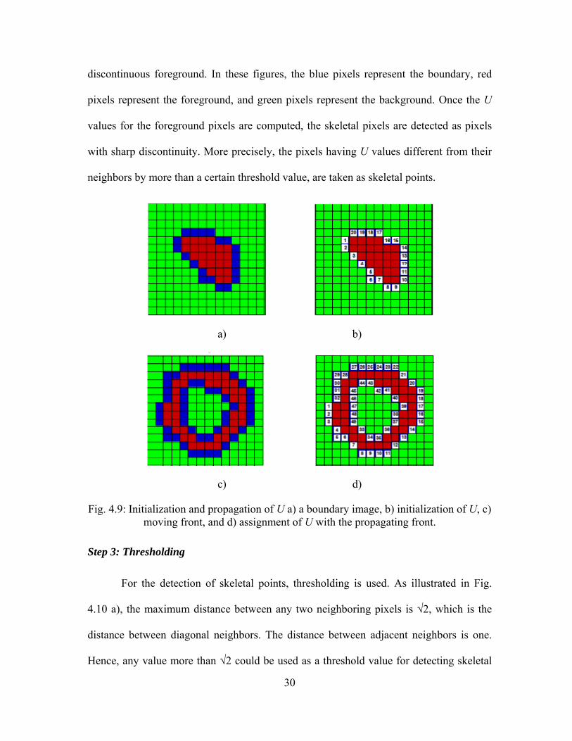
30
discontinuous foreground. In these figures, the blue pixels represent the boundary, red
pixels represent the foreground, and green pixels represent the background. Once the U
values for the foreground pixels are computed, the skeletal pixels are detected as pixels
with sharp discontinuity. More precisely, the pixels having U values different from their
neighbors by more than a certain threshold value, are taken as skeletal points.
a) b)
c) d)
Fig. 4.9: Initialization and propagation of U a) a boundary image, b) initialization of U, c) moving front, and d) assignment of U with the propagating front.
Step 3: Thresholding
For the detection of skeletal points, thresholding is used. As illustrated in Fig.
4.10 a), the maximum distance between any two neighboring pixels is √2, which is the
distance between diagonal neighbors. The distance between adjacent neighbors is one.
Hence, any value more than √2 could be used as a threshold value for detecting skeletal
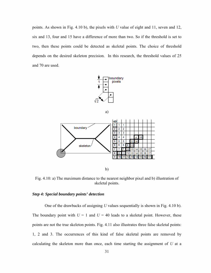
31
points. As shown in Fig. 4.10 b), the pixels with U value of eight and 11, seven and 12,
six and 13, four and 15 have a difference of more than two. So if the threshold is set to
two, then these points could be detected as skeletal points. The choice of threshold
depends on the desired skeleton precision. In this research, the threshold values of 25
and 70 are used.
a)
b)
Fig. 4.10: a) The maximum distance to the nearest neighbor pixel and b) illustration of skeletal points.
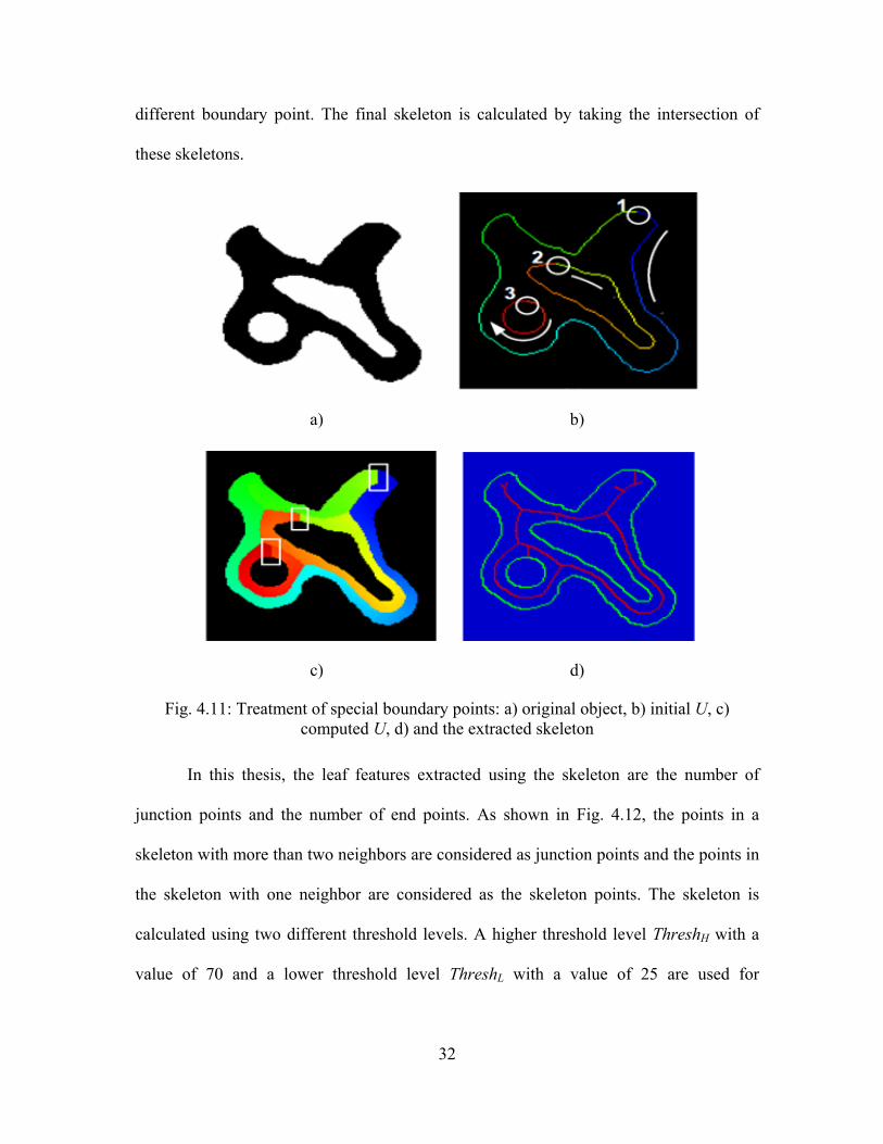
Step 4: Special boundary points’ detection
One of the drawbacks of assigning U values sequentially is shown in Fig. 4.10 b).
The boundary point with U = 1 and U = 40 leads to a skeletal point. However, these
points are not the true skeleton points. Fig. 4.11 also illustrates three false skeletal points:
1, 2 and 3. The occurrences of this kind of false skeletal points are removed by
calculating the skeleton more than once, each time starting the assignment of U at a
32
different boundary point. The final skeleton is calculated by taking the intersection of
these skeletons.
a) b)
c) d)
Fig. 4.11: Treatment of special boundary points: a) original object, b) initial U, c) computed U, d) and the extracted skeleton
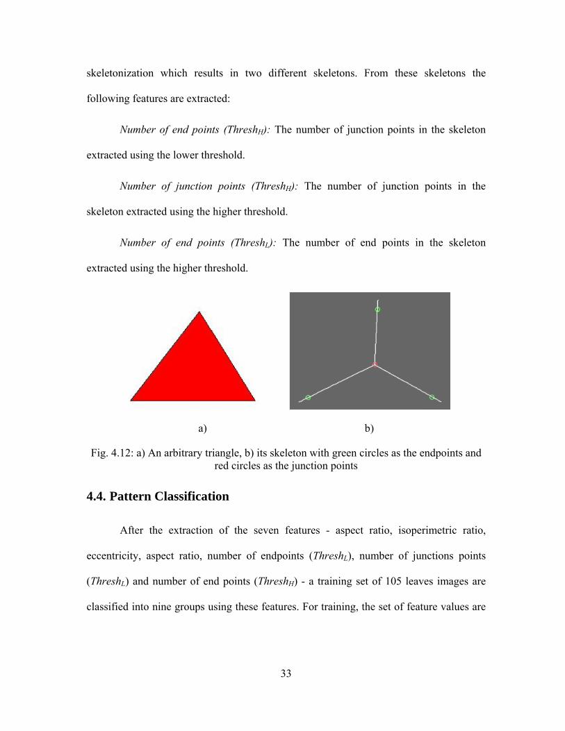
In this thesis, the leaf features extracted using the skeleton are the number of
junction points and the number of end points. As shown in Fig. 4.12, the points in a
skeleton with more than two neighbors are considered as junction points and the points in
the skeleton with one neighbor are considered as the skeleton points. The skeleton is
calculated using two different threshold levels. A higher threshold level ThreshH with a
value of 70 and a lower threshold level ThreshL with a value of 25 are used for
skele
follo
extra
skele
extra
Fig
4.4.
ecce
(Thr
class
etonization
owing featur
Number
acted using t
Number
eton extracte
Number
acted using t
. 4.12: a) An
Pattern C
After the
entricity, asp
reshL) and nu
sified into ni
which resu
es are extrac
of end poin
the lower thr
of junction
ed using the
of end poi
the higher th
a)
n arbitrary tr
Classificat
e extraction
pect ratio, n
umber of en
ine groups u
ults in two
cted:
nts (ThreshH)
reshold.
n points (Th
higher thres
ints (Thresh
hreshold.
riangle, b) itsred circles a
tion
n of the sev
number of e
nd points (Th
using these f
33
different s
): The numb
hreshH): The
shold.
hL): The num
s skeleton was the juncti
ven features
endpoints (T
ThreshH) - a
features. For
skeletons. F
ber of juncti
e number o
mber of en
b
with green ciron points
s - aspect r
ThreshL), nu
training set
r training, th
rom these
ion points in
of junction
nd points in
)
rcles as the e
ratio, isoper
umber of jun
of 105 leav
he set of feat
skeletons th
n the skeleto
points in th
n the skeleto
endpoints an
rimetric rati
nctions poin
ves images a
ture values a
he
on
he
on
nd
io,
nts
are
are
34
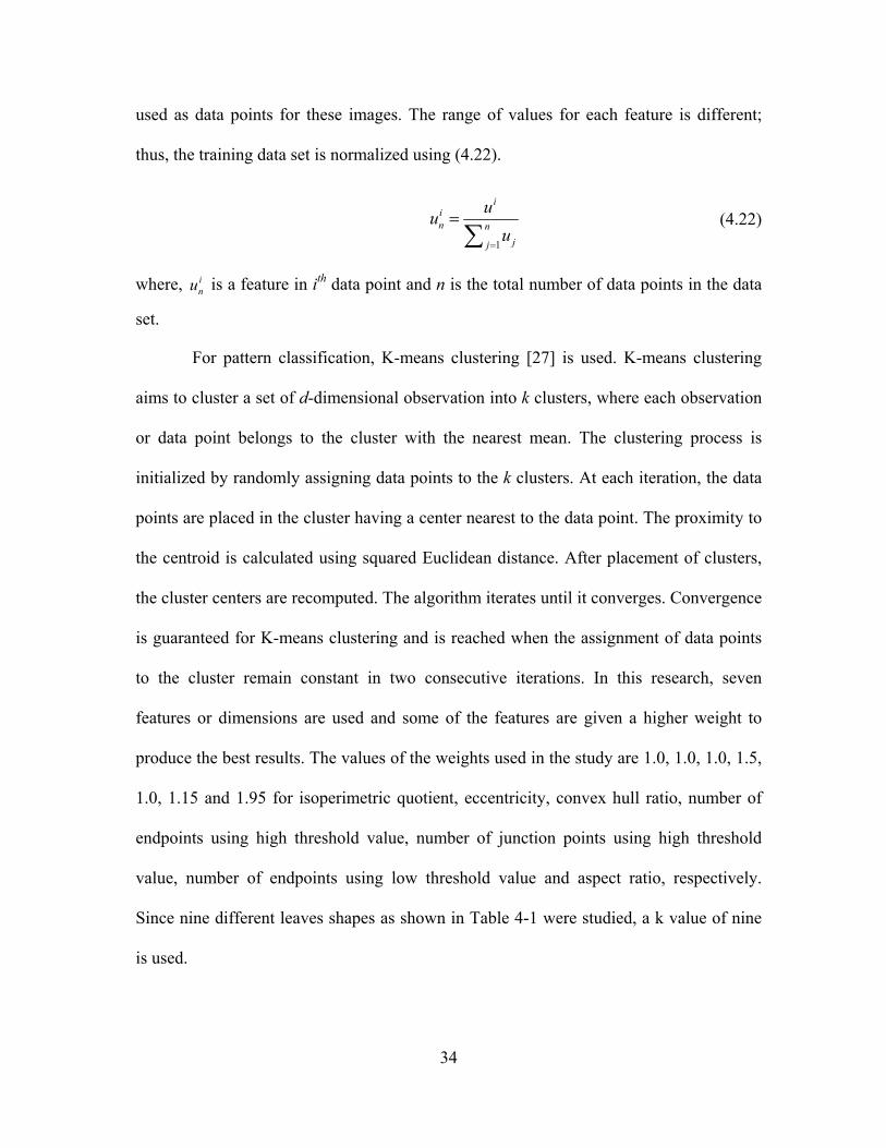
used as data points for these images. The range of values for each feature is different;
thus, the training data set is normalized using (4.22).
1
iin n
jj
uuu
=
=∑
(4.22)
where, inu is a feature in ith data point and n is the total number of data points in the data
set.
For pattern classification, K-means clustering [27] is used. K-means clustering
aims to cluster a set of d-dimensional observation into k clusters, where each observation
or data point belongs to the cluster with the nearest mean. The clustering process is
initialized by randomly assigning data points to the k clusters. At each iteration, the data
points are placed in the cluster having a center nearest to the data point. The proximity to
the centroid is calculated using squared Euclidean distance. After placement of clusters,
the cluster centers are recomputed. The algorithm iterates until it converges. Convergence
is guaranteed for K-means clustering and is reached when the assignment of data points
to the cluster remain constant in two consecutive iterations. In this research, seven
features or dimensions are used and some of the features are given a higher weight to
produce the best results. The values of the weights used in the study are 1.0, 1.0, 1.0, 1.5,
1.0, 1.15 and 1.95 for isoperimetric quotient, eccentricity, convex hull ratio, number of
endpoints using high threshold value, number of junction points using high threshold
value, number of endpoints using low threshold value and aspect ratio, respectively.
Since nine different leaves shapes as shown in Table 4-1 were studied, a k value of nine
is used.
35
Appendix B contains the information about the number of leaves in each group
used in this research. It also contains the name of the plants from which the leaves were
extracted.
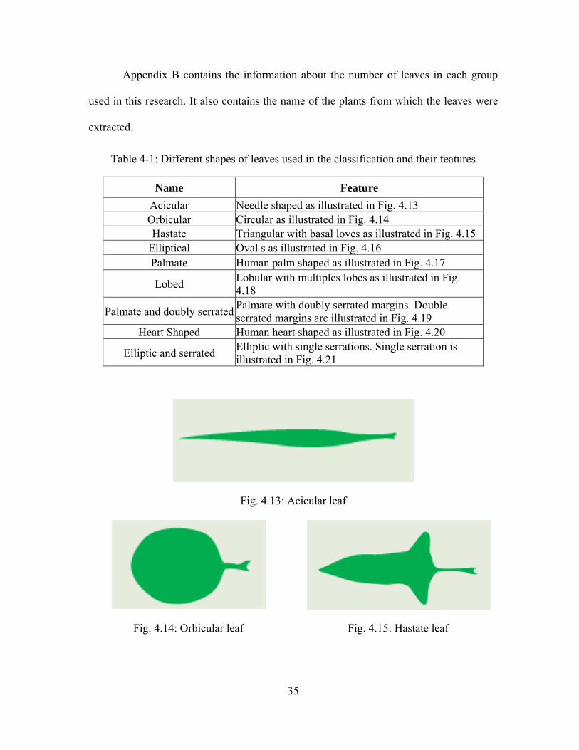
Table 4-1: Different shapes of leaves used in the classification and their features
Name Feature Acicular Needle shaped as illustrated in Fig. 4.13 Orbicular Circular as illustrated in Fig. 4.14 Hastate Triangular with basal loves as illustrated in Fig. 4.15
Elliptical Oval s as illustrated in Fig. 4.16 Palmate Human palm shaped as illustrated in Fig. 4.17
Lobed Lobular with multiples lobes as illustrated in Fig. 4.18
Palmate and doubly serrated Palmate with doubly serrated margins. Double serrated margins are illustrated in Fig. 4.19
Heart Shaped Human heart shaped as illustrated in Fig. 4.20
Elliptic and serrated Elliptic with single serrations. Single serration is illustrated in Fig. 4.21
Fig. 4.13: Acicular leaf
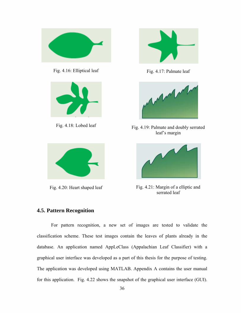
Fig. 4.14: Orbicular leaf
Fig. 4.15: Hastate leaf
36
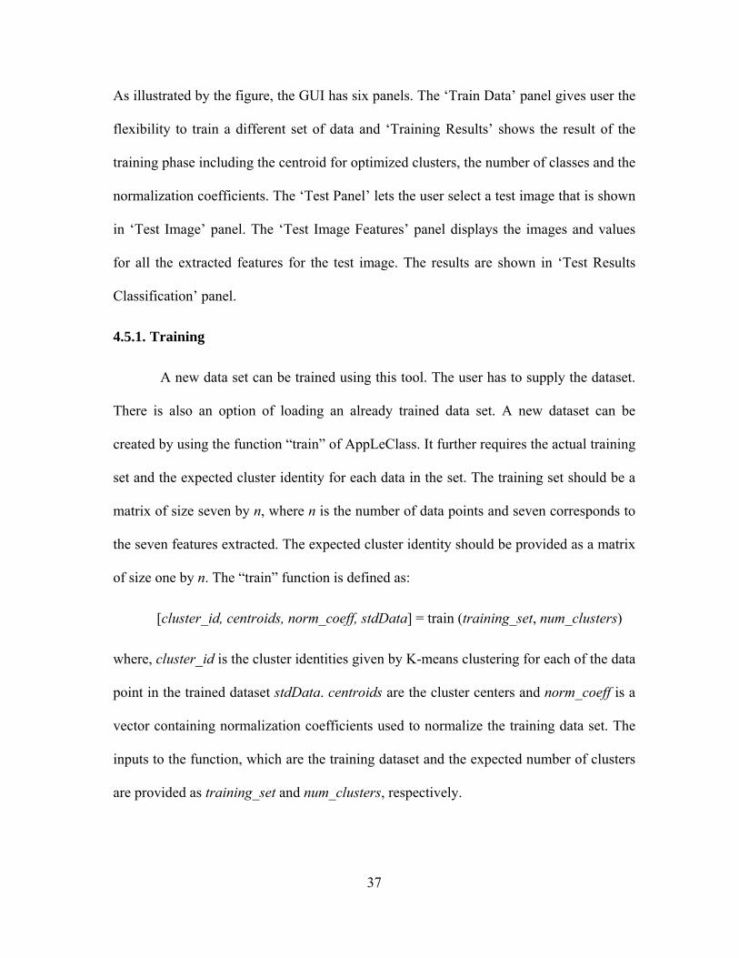
Fig. 4.16: Elliptical leaf
Fig. 4.17: Palmate leaf
Fig. 4.18: Lobed leaf
Fig. 4.19: Palmate and doubly serrated leaf’s margin
Fig. 4.20: Heart shaped leaf
Fig. 4.21: Margin of a elliptic and serrated leaf
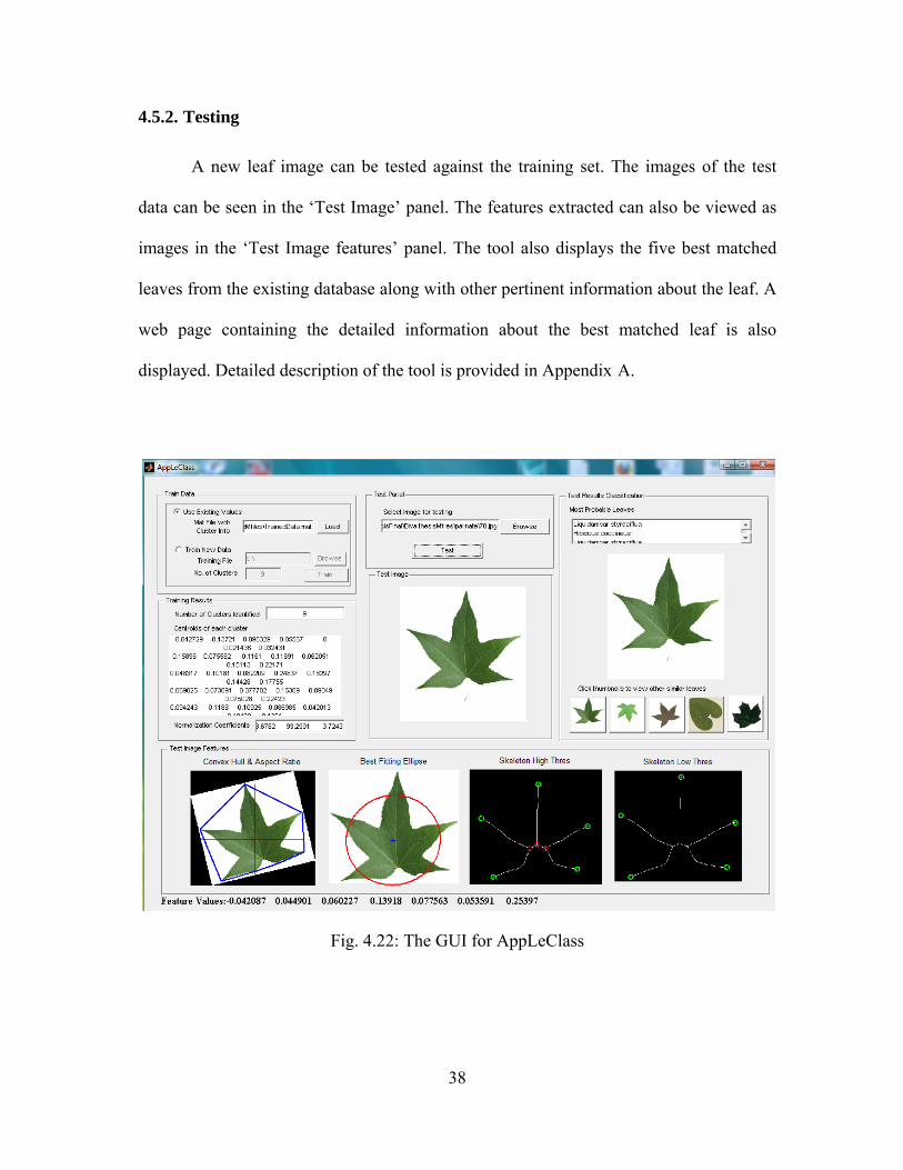
4.5. Pattern Recognition
For pattern recognition, a new set of images are tested to validate the
classification scheme. These test images contain the leaves of plants already in the
database. An application named AppLeClass (Appalachian Leaf Classifier) with a
graphical user interface was developed as a part of this thesis for the purpose of testing.
The application was developed using MATLAB. Appendix A contains the user manual
for this application. Fig. 4.22 shows the snapshot of the graphical user interface (GUI).
37
As illustrated by the figure, the GUI has six panels. The ‘Train Data’ panel gives user the
flexibility to train a different set of data and ‘Training Results’ shows the result of the
training phase including the centroid for optimized clusters, the number of classes and the
normalization coefficients. The ‘Test Panel’ lets the user select a test image that is shown
in ‘Test Image’ panel. The ‘Test Image Features’ panel displays the images and values
for all the extracted features for the test image. The results are shown in ‘Test Results
Classification’ panel.
4.5.1. Training
A new data set can be trained using this tool. The user has to supply the dataset.
There is also an option of loading an already trained data set. A new dataset can be
created by using the function “train” of AppLeClass. It further requires the actual training
set and the expected cluster identity for each data in the set. The training set should be a
matrix of size seven by n, where n is the number of data points and seven corresponds to
the seven features extracted. The expected cluster identity should be provided as a matrix
of size one by n. The “train” function is defined as:
[cluster_id, centroids, norm_coeff, stdData] = train (training_set, num_clusters)
where, cluster_id is the cluster identities given by K-means clustering for each of the data
point in the trained dataset stdData. centroids are the cluster centers and norm_coeff is a
vector containing normalization coefficients used to normalize the training data set. The
inputs to the function, which are the training dataset and the expected number of clusters
are provided as training_set and num_clusters, respectively.
38
4.5.2. Testing
A new leaf image can be tested against the training set. The images of the test
data can be seen in the ‘Test Image’ panel. The features extracted can also be viewed as
images in the ‘Test Image features’ panel. The tool also displays the five best matched
leaves from the existing database along with other pertinent information about the leaf. A
web page containing the detailed information about the best matched leaf is also
displayed. Detailed description of the tool is provided in Appendix A.
Fig. 4.22: The GUI for AppLeClass
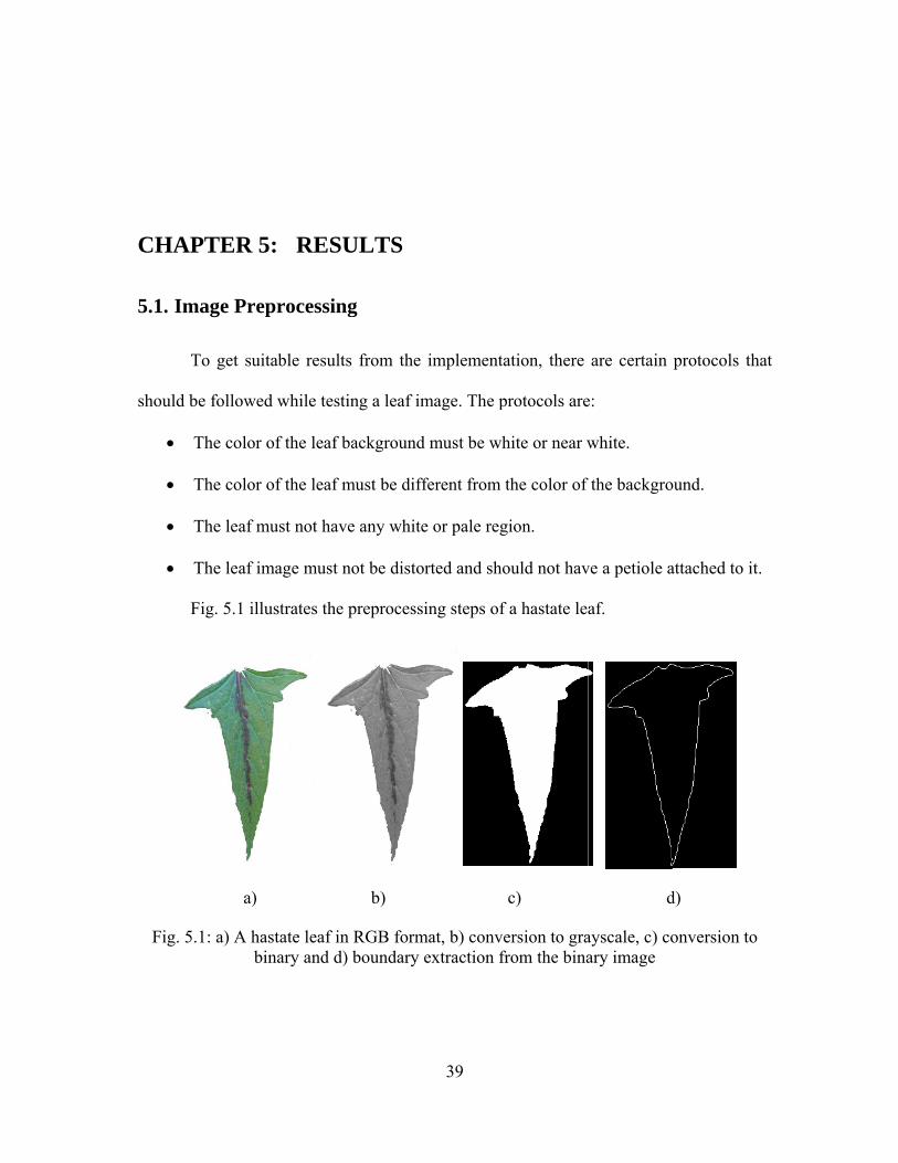
CH
5.1.
shou
•
•
•
•
Fig
HAPTER
Image Pr
To get su
uld be follow
• The colo
• The colo
• The leaf
• The leaf
Fig. 5.1 i
a)
g. 5.1: a) A h
R 5: RES
reprocessi
uitable resul
wed while tes
or of the leaf
or of the leaf
f must not ha
f image must
illustrates th
)
hastate leaf ibinary and d
SULTS
ng
lts from the
sting a leaf i
f background
f must be dif
ave any whit
t not be disto
e preprocess
b)
in RGB formd) boundary
39
e implementa
mage. The p
d must be wh
fferent from
te or pale reg
orted and sho
sing steps of
mat, b) conveextraction f
ation, there
protocols are
hite or near w
the color of
gion.
ould not hav
f a hastate le
c)
ersion to grafrom the bina
are certain
e:
white.
f the backgro
ve a petiole a
af.
d
ayscale, c) coary image
protocols th
ound.
attached to it
d)
onversion to
hat
t.
o
40
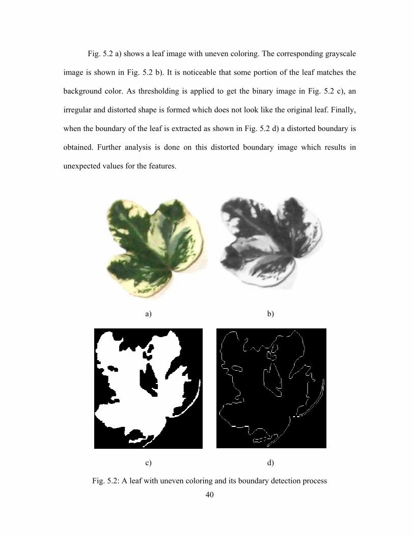
Fig. 5.2 a) shows a leaf image with uneven coloring. The corresponding grayscale
image is shown in Fig. 5.2 b). It is noticeable that some portion of the leaf matches the
background color. As thresholding is applied to get the binary image in Fig. 5.2 c), an
irregular and distorted shape is formed which does not look like the original leaf. Finally,
when the boundary of the leaf is extracted as shown in Fig. 5.2 d) a distorted boundary is
obtained. Further analysis is done on this distorted boundary image which results in
unexpected values for the features.
a) b)
c) d)
Fig. 5.2: A leaf with uneven coloring and its boundary detection process
41
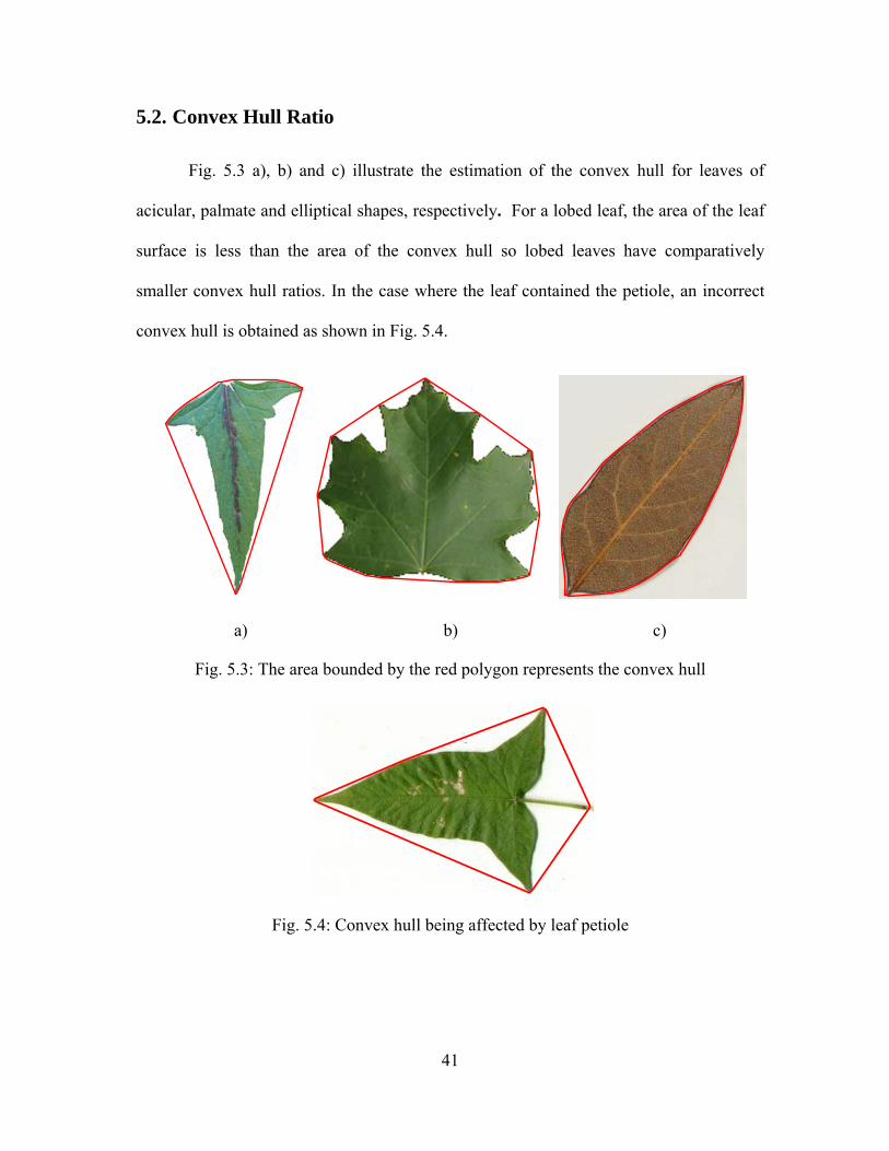
5.2. Convex Hull Ratio
Fig. 5.3 a), b) and c) illustrate the estimation of the convex hull for leaves of
acicular, palmate and elliptical shapes, respectively. For a lobed leaf, the area of the leaf
surface is less than the area of the convex hull so lobed leaves have comparatively
smaller convex hull ratios. In the case where the leaf contained the petiole, an incorrect
convex hull is obtained as shown in Fig. 5.4.
a) b) c)
Fig. 5.3: The area bounded by the red polygon represents the convex hull
Fig. 5.4: Convex hull being affected by leaf petiole
42
5.3. Isoperemetric Quotient
Results of isoperemetric quotient extraction shows that leaves with irregular
boundaries have smaller isoperemetric quotients which is attributed to the fact that they
have larger value for perimeter. Compared to leaves with irregular boundary, the leaves
with regular boundary have smaller isoperemetric quotients. There are no errors related to
the calculation of isoperimetric quotient except for the case where the leaf boundary is
distorted as seen in Fig. 5.2.
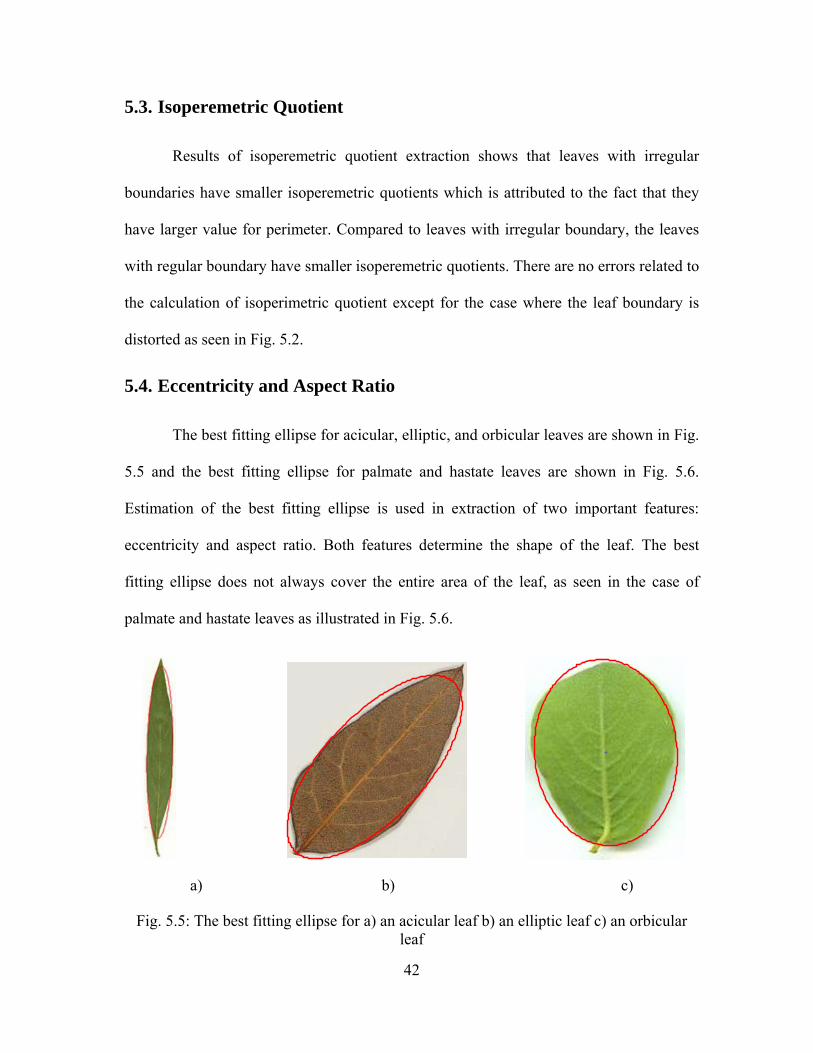
5.4. Eccentricity and Aspect Ratio
The best fitting ellipse for acicular, elliptic, and orbicular leaves are shown in Fig.
5.5 and the best fitting ellipse for palmate and hastate leaves are shown in Fig. 5.6.
Estimation of the best fitting ellipse is used in extraction of two important features:
eccentricity and aspect ratio. Both features determine the shape of the leaf. The best
fitting ellipse does not always cover the entire area of the leaf, as seen in the case of
palmate and hastate leaves as illustrated in Fig. 5.6.
a) b) c)
Fig. 5.5: The best fitting ellipse for a) an acicular leaf b) an elliptic leaf c) an orbicular leaf
43
a) b)
Fig. 5.6: The best fitting ellipse for a) a palmate leaf b) a hastate leaf
5.5. Skeleton
The number of end points and the number of junction points obtained from the
skeleton calculation using a high threshold value of 70 are used to determine the number
of lobes in the leaf. Furthermore, the number of end points extracted from a skeleton
using a low threshold value of 25 provides some information on the type of margins of
the leaf. Results show that marginated leaves produce a higher number of end points
when skeletonized using the lower threshold.
Fig. 5.7 shows the skeletal calculation of an acicular leaf using high and low
threshold values. Similarly, Fig. 5.8 shows the skeletal calculation of a hastate leaf. In
Fig. 5.7 through Fig. 5.12, green circles represent the end points and red circles represent
the junction points. In both acicular and hastate leaves, skeletonization with higher
threshold and lower threshold values produce similar skeleton, thus indicating that these
leaves are not marginated. On the other hand, as illustrated in Fig. 5.9, if a leaf is
marg
leaf
5.16
respe
extra
skele
num
resul
valu
not s
leave
high
orbic
Fig
ginated, then
without mar
which show
ectively. It
actable from
etonization
mber of endp
lts are obta
es. The resu
sufficient fo
es with serra
h as well as
cular leaf in
a
g. 5.7: a) An
n it results i
rgins. The sa
w the skeleto
should be n
m the skel
of a serrated
points than
ained when
ults for this c
or distinguish
ations are als
with the low
Fig. 5.11 an
a)
acicular leaf
in a differen
ame conclusi
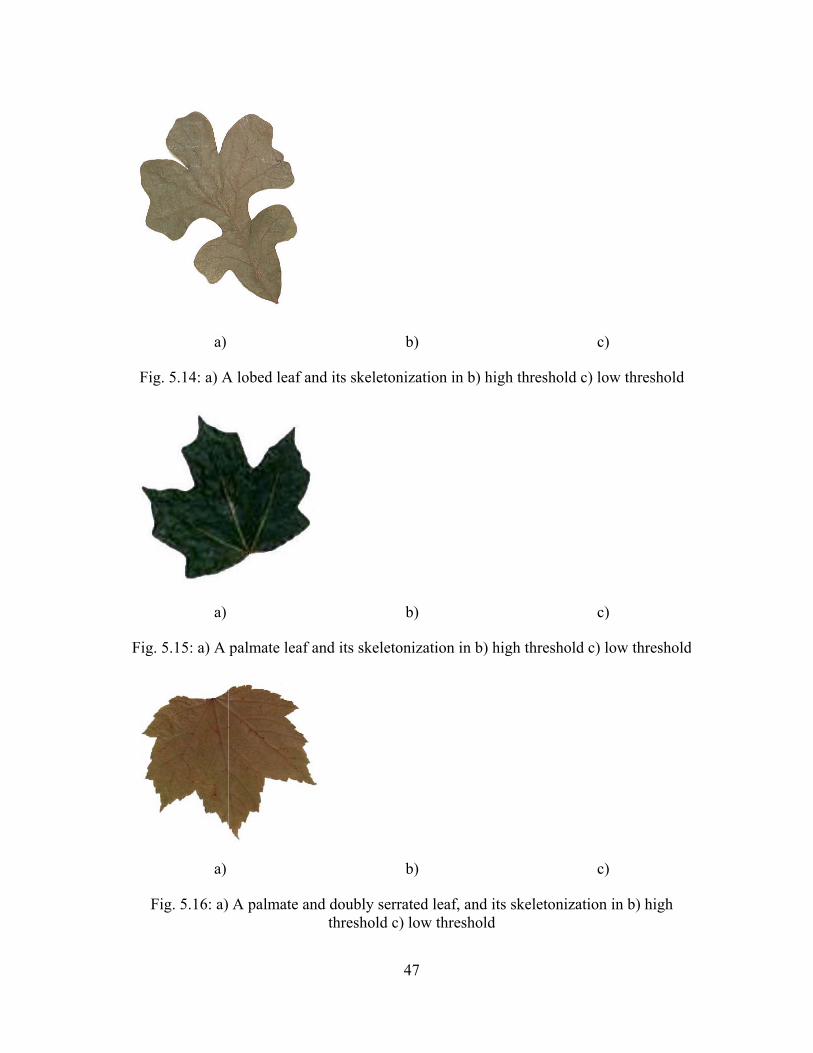
onization of
noted that th
eton for lo
d lobed leaf
skeletoniza
a lobed lea
case are illus
hing a lobed
so considere
w threshold
nd Fig. 5.12,
f and its skel
44
nt skeletal st
ions can be m
a palmate le
he informatio
obed leaves
f at the low
ation under
af is skeleto
strated in Fi
d leaf from
ed in the lobe
values are s
respectively
b)
letonization
tructure than
made by com
eaf and a dou
on about ser
s. As illust
wer threshold
the higher
onized using
g. 5.14. Hen
a serrated lo
ed group. Sk
shown for a
y.
in b) high th
n that of a s
mparing Fig.
ubly serrated
rrations of m
trated in F
d value prod
threshold v
g high and
nce skeletal
obed leaf; th
keletal extrac
a heart-shape
c)
hreshold c) l
similar shap
. 5.15 and Fi
d palmate le
margins is n
Fig. 5.13, th
duces a larg
value. Simil
low thresho
information
hus, the lob
ctions with th
ed leaf and
low threshold
ed
ig.
eaf
not
he
ger
lar
old
is
ed
he
an
d
Fi
Fig.
Fig
a)
g. 5.8: a) A
a)
5.9: a) An e
a)
. 5.10: a) An
hastate leaf
elliptic and si
n elliptic leaf
and its skele
ingly serratec) l
f and its ske
45
b)
etonization in
b)
ed leaf, and ilow threshold
b)
letonization
n b) high thr
its skeletonizd
in b) high th
c)
reshold c) lo
c)
zation in b) h
c)
hreshold c) l
)
ow threshold
)
high thresho
)
low threshol
d
old
d
F
Fig.
a)
Fig. 5.11: a)
a)
Fig. 5.12: a
a)
. 5.13: a) A l
A heart shap
a) An orbicul
lobed and se
ped leaf and
lar leaf and i
errated leaf, a
46
b)
d its skeletonthreshold
b)
its skeletonizthreshold
b)
and its skelethreshold
nization in b)
zation in b) h
etonization in
c)
) high thresh
c)
high thresho
c)
n b) high thr
)
hold c) low
)
old c) low
)
reshold c) low
w
Fi
Fig
F
a)
ig. 5.14: a) A
a)
g. 5.15: a) A
a)
Fig. 5.16: a)
A lobed leaf
palmate leaf
A palmate a
and its skele
f and its skel
and doubly sthreshold
47
b)
etonization in
b)
letonization
b)
serrated leafd c) low thre
n b) high thr
in b) high th
f, and its skeleshold
c)
reshold c) lo
c)
hreshold c) l
c)
letonization
)
ow threshold
)
low threshold
)
in b) high
d
48
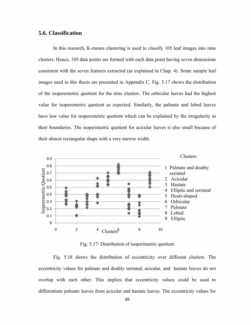
5.6. Classification
In this research, K-means clustering is used to classify 105 leaf images into nine
clusters. Hence, 105 data points are formed with each data point having seven dimensions
consistent with the seven features extracted (as explained in Chap. 4). Some sample leaf
images used in this thesis are presented in Appendix C. Fig. 5.17 shows the distribution
of the isoperemetric quotient for the nine clusters. The orbicular leaves had the highest
value for isoperemetric quotient as expected. Similarly, the palmate and lobed leaves
have low value for isoperemetric quotient which can be explained by the irregularity in
their boundaries. The isoperimetric quotient for acicular leaves is also small because of
their almost rectangular shape with a very narrow width.
Fig. 5.17: Distribution of isoperimetric quotient
Fig. 5.18 shows the distribution of eccentricity over different clusters. The
eccentricity values for palmate and doubly serrated, acicular, and hastate leaves do not
overlap with each other. This implies that eccentricity values could be used to
differentiate palmate leaves from acicular and hastate leaves. The eccentricity values for
0
0.1
0.2
0.3
0.4
0.5
0.6
0.7
0.8
0.9
0 2 4 6 8 10
Isop
erem
etric
Quo
tient
Clusters
Clusters
1 Palmate and doublyserrated
2 Acicular3 Hastate4 Elliptic and serrated5 Heart-shaped6 Orbicular7 Palmate8 Lobed9 Elliptic
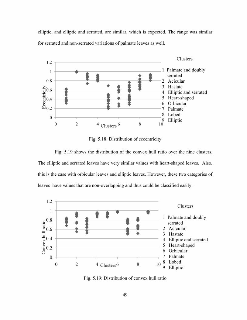
ellip
for s
The
this
leave
Ecce
ntric
ityC
onve
x hu
ll ra
tio
ptic, and ellip
serrated and
Fig. 5.1
elliptic and
is the case w
es have valu
0
0.2
0.4
0.6
0.8
1
1.2
0
y
0
0.2
0.4
0.6
0.8
1
1.2
0
ptic and ser
non-serrated
Fi
19 shows the
serrated lea
with orbicula
ues that are n
Fig.
2
2
rrated, are si
d variations o
ig. 5.18: Dis
e distributio
aves have ve
ar leaves and
non-overlapp
5.19: Distrib
4 Clusters
4 Clusters
49
imilar, whic
of palmate le
tribution of
n of the con
ry similar va
d elliptic leav
ping and thu
bution of con
6s
6 8s
h is expecte
eaves as wel
eccentricity
nvex hull rat
alues with h
ves. Howeve
us could be c
nvex hull rat
8 10
8 10
ed. The rang
ll.
tio over the
heart-shaped
er, these two
classified eas
tio
0
Clus
1 Palmate aserrated
2 Acicular3 Hastate4 Elliptic a5 Heart-sh6 Orbicula7 Palmate8 Lobed9 Elliptic
Clus
1 Palmate aserrated
2 Acicular3 Hastate4 Elliptic a5 Heart-sh6 Orbicula7 Palmate8 Lobed9 Elliptic
ge was simil
nine cluster
leaves. Als
o categories
sily.
sters
and doubly
and serratedaped
ar
sters
and doubly
r
and serratedhapedar
lar
rs.
so,
of
50
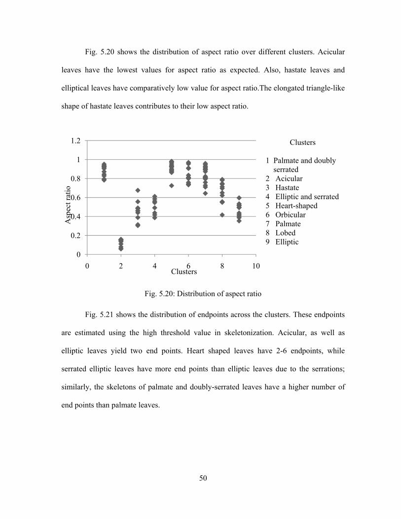
Fig. 5.20 shows the distribution of aspect ratio over different clusters. Acicular
leaves have the lowest values for aspect ratio as expected. Also, hastate leaves and
elliptical leaves have comparatively low value for aspect ratio.The elongated triangle-like
shape of hastate leaves contributes to their low aspect ratio.
Fig. 5.20: Distribution of aspect ratio
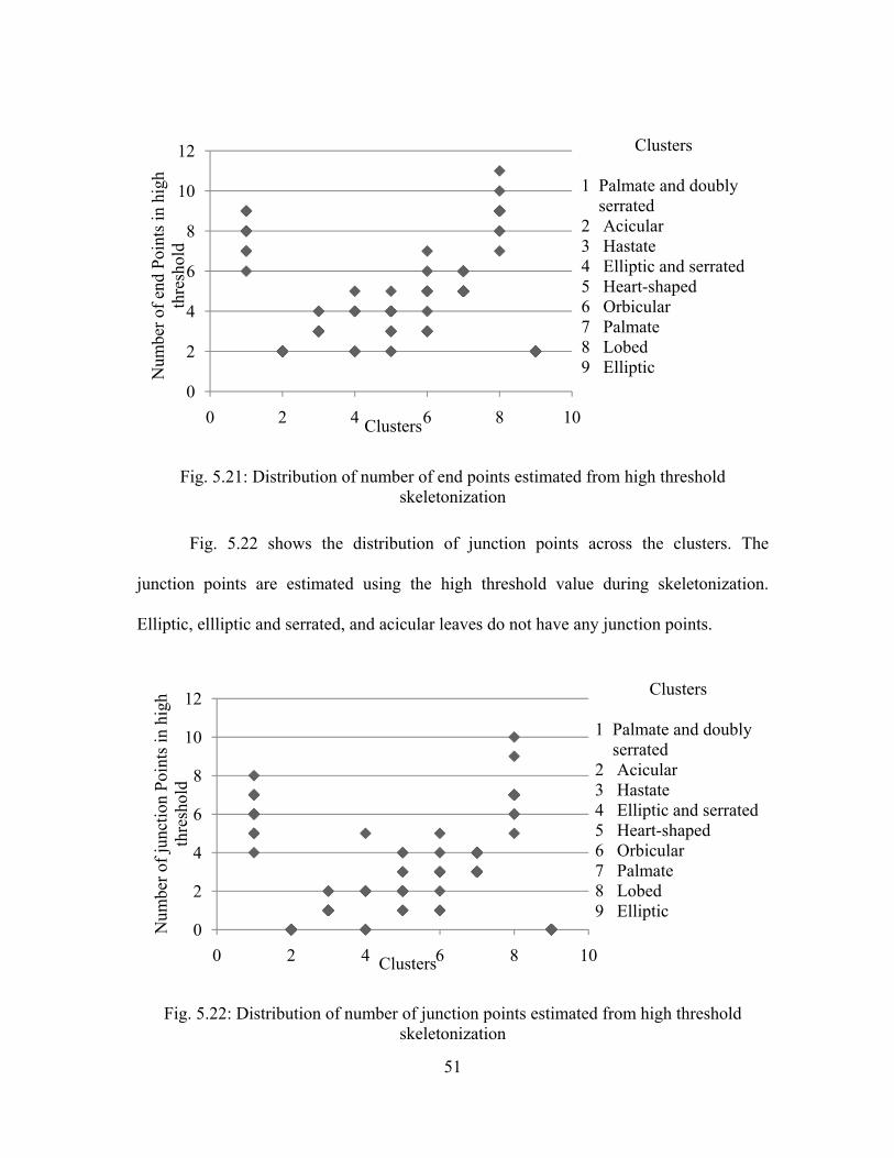
Fig. 5.21 shows the distribution of endpoints across the clusters. These endpoints
are estimated using the high threshold value in skeletonization. Acicular, as well as
elliptic leaves yield two end points. Heart shaped leaves have 2-6 endpoints, while
serrated elliptic leaves have more end points than elliptic leaves due to the serrations;
similarly, the skeletons of palmate and doubly-serrated leaves have a higher number of
end points than palmate leaves.
0
0.2
0.4
0.6
0.8
1
1.2
0 2 4 6 8 10
Asp
ect r
atio
Clusters
Clusters
1 Palmate and doublyserrated
2 Acicular3 Hastate4 Elliptic and serrated5 Heart-shaped6 Orbicular7 Palmate8 Lobed9 Elliptic
51
Fig. 5.21: Distribution of number of end points estimated from high threshold skeletonization
Fig. 5.22 shows the distribution of junction points across the clusters. The
junction points are estimated using the high threshold value during skeletonization.
Elliptic, ellliptic and serrated, and acicular leaves do not have any junction points.
Fig. 5.22: Distribution of number of junction points estimated from high threshold skeletonization
0
2
4
6
8
10
12
0 2 4 6 8 10
Num
ber o
f end
Poi
nts i
n hi
gh
thre
shol
d
Clusters
Clusters
1 Palmate and doublyserrated
2 Acicular3 Hastate4 Elliptic and serrated5 Heart-shaped6 Orbicular7 Palmate8 Lobed9 Elliptic
0
2
4
6
8
10
12
0 2 4 6 8 10
Num
ber o
f jun
ctio
n Po
ints
in h
igh
thre
shol
d
Clusters
Clusters
1 Palmate and doubly serrated
2 Acicular3 Hastate4 Elliptic and serrated5 Heart-shaped6 Orbicular7 Palmate8 Lobed9 Elliptic
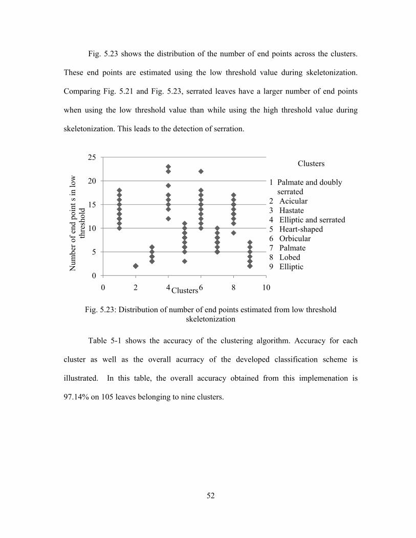
52
Fig. 5.23 shows the distribution of the number of end points across the clusters.
These end points are estimated using the low threshold value during skeletonization.
Comparing Fig. 5.21 and Fig. 5.23, serrated leaves have a larger number of end points
when using the low threshold value than while using the high threshold value during
skeletonization. This leads to the detection of serration.
Fig. 5.23: Distribution of number of end points estimated from low threshold skeletonization
Table 5-1 shows the accuracy of the clustering algorithm. Accuracy for each
cluster as well as the overall acurracy of the developed classification scheme is
illustrated. In this table, the overall accuracy obtained from this implemenation is
97.14% on 105 leaves belonging to nine clusters.
0
5
10
15
20
25
0 2 4 6 8 10
Num
ber o
f end
poi
nt s
in lo
w
thre
shol
d
Clusters
Clusters
1 Palmate and doublyserrated
2 Acicular3 Hastate4 Elliptic and serrated5 Heart-shaped6 Orbicular7 Palmate8 Lobed9 Elliptic
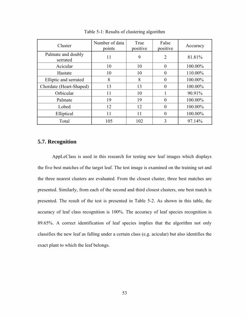
53
Table 5-1: Results of clustering algorithm
Cluster Number of data points
True positive
False positive Accuracy
Palmate and doubly serrated 11 9 2 81.81%
Acicular 10 10 0 100.00% Hastate 10 10 0 110.00%
Elliptic and serrated 8 8 0 100.00% Chordate (Heart-Shaped) 13 13 0 100.00%
Orbicular 11 10 1 90.91% Palmate 19 19 0 100.00% Lobed 12 12 0 100.00%
Elliptical 11 11 0 100.00% Total 105 102 3 97.14%
5.7. Recognition
AppLeClass is used in this research for testing new leaf images which displays
the five best matches of the target leaf. The test image is examined on the training set and
the three nearest clusters are evaluated. From the closest cluster, three best matches are
presented. Similarly, from each of the second and third closest clusters, one best match is
presented. The result of the test is presented in Table 5-2. As shown in this table, the
accuracy of leaf class recognition is 100%. The accuracy of leaf species recognition is
89.65%. A correct identification of leaf species implies that the algorithm not only
classifies the new leaf as falling under a certain class (e.g. acicular) but also identifies the
exact plant to which the leaf belongs.
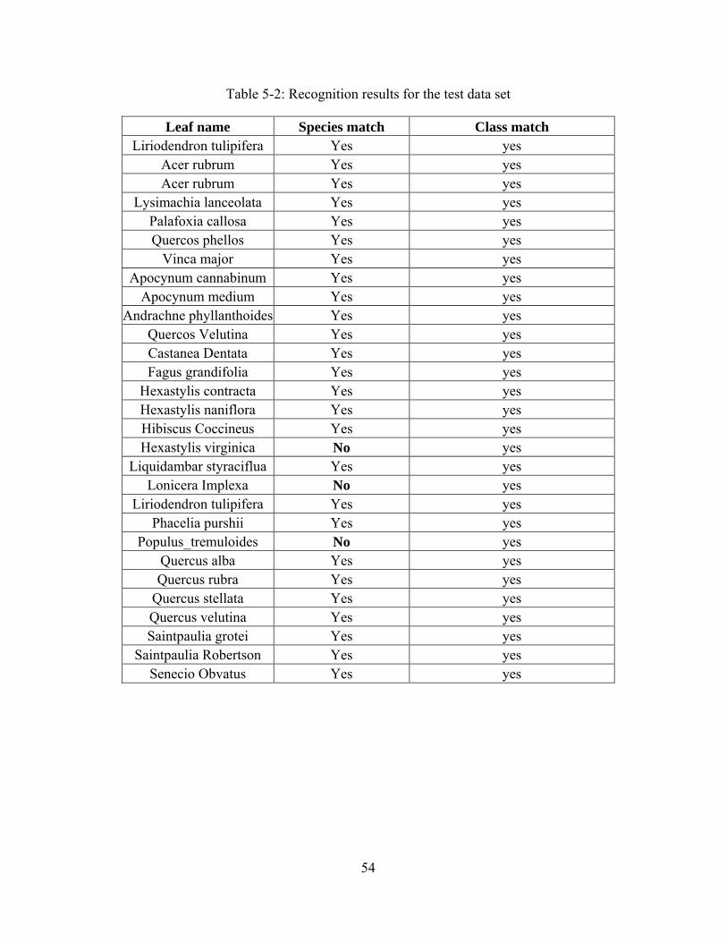
54
Table 5-2: Recognition results for the test data set
Leaf name Species match Class match Liriodendron tulipifera Yes yes
Acer rubrum Yes yes Acer rubrum Yes yes
Lysimachia lanceolata Yes yes Palafoxia callosa Yes yes Quercos phellos Yes yes
Vinca major Yes yes Apocynum cannabinum Yes yes
Apocynum medium Yes yes Andrachne phyllanthoides Yes yes
Quercos Velutina Yes yes Castanea Dentata Yes yes Fagus grandifolia Yes yes
Hexastylis contracta Yes yes Hexastylis naniflora Yes yes Hibiscus Coccineus Yes yes Hexastylis virginica No yes
Liquidambar styraciflua Yes yes Lonicera Implexa No yes
Liriodendron tulipifera Yes yes Phacelia purshii Yes yes
Populus_tremuloides No yes Quercus alba Yes yes Quercus rubra Yes yes
Quercus stellata Yes yes Quercus velutina Yes yes Saintpaulia grotei Yes yes
Saintpaulia Robertson Yes yes Senecio Obvatus Yes yes
55
CHAPTER 6: Conclusions and Future Recommendations
6.1. Conclusion
In this research, various features related to the shape of the leaves were studied
and the most appropriate features were used for leaf image-based plant classification. The
features selected in this automated plant identification were: 1) isoperimetric quotient, 2)
convex hull ratio, 3) aspect ratio, 4) eccentricity and 5) number of endpoints and junction
points in the skeleton of the leaf. These features were vital in identifying leaf shapes,
number of lobes and margin types. Leaves of nine classes were used and a classifier was
implemented and tested using 105 leaves of 38 different species.
6.1.1. Isoperemetric Quotient
The isoperemetric quotient was obtained by calculating the area and the perimeter
of the leaf. Area was calculated by counting the number of pixels in the foreground.
Similarly, perimeter was calculated by counting the number of pixels in the boundary of
the leaf. From the results of this research, observations were made that the isoperemetric
quotient is greater for circular leaves with regular margins. Elongated leaves and leaves
with irregular margins had a comparatively lower isoperemetric quotient than other
leaves.
56
6.1.2. Eccentricity and Aspect Ratio
For calculation of eccentricity, the best fitting ellipse was estimated using the
central moment of the leaf shape, which is a region-based method. A region-based
method was used instead of a boundary-based method because the region based method
was not sensitive to the irregularities in boundary of a shape. From the best fit ellipse, the
aspect ratio was also calculated. The results of the research show that eccentricity and
aspect ratio together were important in differentiating elongated leaves from circular
leaves. Aspect ratio and eccentricity were not sensitive to the margin information.
6.1.3. Convex Hull Ratio
The convex hull was calculated using Andrew’s monotone chain algorithm.
Andrew’s monotone chain algorithm worst case scenario performance was equal to the
regular Graham’s scan’s performance.
The results of this research showed that leaves without lobes and leaves with
regular boundaries have a lower convex hull ratio than leaves with irregular boundaries
and leaves with lobes.
6.1.4. Skeleton
The skeleton was calculated using an augmented fast marching method. The
results from the skeleton extracted in higher threshold were important in distinguishing
the number of lobes in a leaf. Elliptic leaves had two endpoints, and heart-shaped leaves
had three endpoints and one junction point. The number of endpoint and junction points
increased with the increase in the number of lobes. Similarly, skeleton extracted in lower
57
threshold gave some information about the boundary margins. More endpoints were
detected in palmate leaves with serrations than those in palmate leaves when skeletonized
using lower threshold.
6.1.5. Summary
All the traninng and testing was done using the application AppLeClass which
was developed as a part of the research. The tool has all the functionalities required for
testing and training. AppLeClass displays the features extracted for an image and
displays the five best matches of the target leaf. Hence, calculation of efficiency and
error was simplified and studying a pattern in the erroneous cases was convenient.
The results for the training set of images used in this research indicates an
accuracy of 97.14% for the classification algorithm. Results from the test data set show
that the classification algorithm identifies the class of these leaves 100% of the time
whereas the accuracy in identifying the exact species of the leaf was 89.65%.
The errors in identification mostly corresponded to two inaccuracies during the
image processing stage. The first incurracy was in identifying the correct type of margins.
The error propagated to the feature extraction phase. This kind of error was prominent in
leaves with very subtle margins. The second incurracy was seen in extracting the number
of lobes using the skeleton. The skeleton approach was found to be sensitive to leaf
curvature, thus sometimes giving erroneous output for lobe identification.
6.2. Future Recommendations
The research can be improved using a larger training set with other leaf shapes. In
the data collection phase, leaves were cut from a herbarium specimen manually and the

58
noise in the leaf background was removed manually. These processes can be automated
for future analyses.
The features used in this research were not robust for leaves with irregular
margins. Further analyses can be conducted to improve the current feature extraction
process and to include additional features to make the agorithm robust for all kinds of
leaf.
59
BIBLIOGRAPHY
[1] W. E. Snyder and H Qi, Machine Vision, Cambridge, MA: Cambridge university press, 2004.
[2] M. J. Dallwitz (1980). A general system for coding taxonomic description [online]. vol. 29. Available:http://delta-intkey.com
[3] D. Warren, “Automated leaf shape description for variety testing in chrysanthemums,” in Proc. 6th Int. Conf. Image Process. and Its Applicat., Duplin, Ireland, 1997.
[4] Z. Miao et al., “An oopr-based rose variety recognition system,” Engineering Applications of Artificial Intelligence, vol. 19, issue 5, Amsterdam, Elsevier, 2006, pp. 78-101.
[5] B. C. Heymans et al., “A neural network for Opuntia leaf-form recognition,” IJCNN, vol. 3, pp. 2116-2121, 1991.
[6] T. Satioh and T. Kaneko, “Automatic Recognition of Wild Flowers”, ICPR, vol. 2, pp. 2507-2510, 2000.
[7] Y. Li et al., “A leaf vein extraction method based on snakes technique,” in Proc. Neural Networks and Brain Int. Conf., Beijing, China, 2005.
[8] M. Kass et al., “Snakes: active contour models,” in Int. Journal of Computer Vision, vol. 1, Boston, MA: Kluwer Academic Publishers, 1987, pp. 321–331.
[9] H. Fu and Z. Chi, “Combined thresholding and neural network approach for vein pattern extraction from leaf images,” IEE Proc. Vision, Image and Signal Process., vol. 153, issue 6, 2006, pp. 881-892.
[10] H. Qi and J. G. Yang, “Saw tooth feature extraction of leaf edge based on support vector machine,” ICMLC, vol. 5, pp. 3039-3044, 2003.
[11] Y. Nam et al., “Elis: An efficient leaf image retrieval system”, in Proc. Advances in Pattern Recognition Int. Conf., Kolkata, India, 2005.
[12] H. Fu and J. Chi, “A two-stage approach for leaf vein extraction,” ICNNSP, vol. 1, pp. 208-211, 2003.
[13] X. Gu et al.,. Wang, “Leaf recognition based on the combination of wavelet transform and gaussian interpolation,” ICIS, vol. 3644/2005, pp. 253-262, 2005.
[14] J. X. Du et al., “Leaf shape based plant species recognition,” Applied Mathematics and Computation, vol. 185, issue 2, Amsterdam, Elsevier, 2007, pp. 883-893.
60
[15] H. Fu et al., “Machine learning techniques for ontology-based leaf classification,” ICARCV, vol. 1, pp681-686, 2004.
[16] X. F. Wang et al., “Recognition of leaf images based on shape features using a hypersphere classifier,” ICIC, vol. 3644/2005, pp. 87-96, 2005.
[17] S. Wu et al., “A Leaf Recognition Algorithm for Plant Classification Using Probabilistic Neural Network,” in Proc. Signal Process. and Inform. Technology, IEEE Int. Symp., Cairo, Egypt, 2007.
[18] A. Talea, “An augmented fast marching method for computing skeleton and centerlines,” in IEEE TCVG Sym. Visualization, Barcelona, 2002.
[19] H. Blum, “A transformation for extracting new descriptors of shape,” in Models for the Perception of Speech and Visual Form, Cambridge, MA: MIT Press, 1967, pp. 360-380.
[20] H. Blum and R. N. Nagel, “Shape description using weighted symmetric axis features,” in Pattern Recognition, vol. 10, issue 3, Amsterdam, Elsevier, 1978, pp. 167-180.
[21] R. L. Ogniewicz, “Automatic Medial Axis Pruning by Mapping Characteristics of Boundaries Evolving under the Euclidean Geometric Heat Flow onto Voronoi Skeletons,” Harvard Robotics Lab., Cambridge, MA, Tech. Rep. 95-4, 1995.
[22] J. A. Sethian, “A Fast Marching Level Set Method for Monotonically Advancing Fronts,” PNAS, vol. 40, pp. 1528-1538, 1995.
[23] S. Wu and A. Amin, “Automatic Thresholding of Gray-level Using Multi-stage approach,” IEEE Trans Syst Man Cybern, vol. 9, issue 1, pp. 62-66, 1979.
[24] J. Canny, “A Computational Approach to Edge Detection,” IEEE Trans. Pattern Anal. Mach. Intell., vol. 8, issue 6, pp. 679-698, 1986.
[25] A. M. Andrew, “Another Efficient Algorithm for Convex Hulls in Two Dimensions," Inform. Process. Lett., vol. 9, issue 5, pp. 216-219, 1979.
[26] R. L. Graham, “An Efficient Algorithm for Determining the Convex Hull of a Finite Planar Set,” Inform. Process. Lett., vol. 1, issue 4, Amsterdam, Elsevier, 1996, pp. 132-133.
[27] J. B. MacQueen, “Some methods for classification and Analysis Multivariate Observations,” in Proc. 5th Berkeley Symp. Math. Stat. and Probability, Berkley, CA, 1967.
61
APPENDIX A
User Manual for AppLeClass
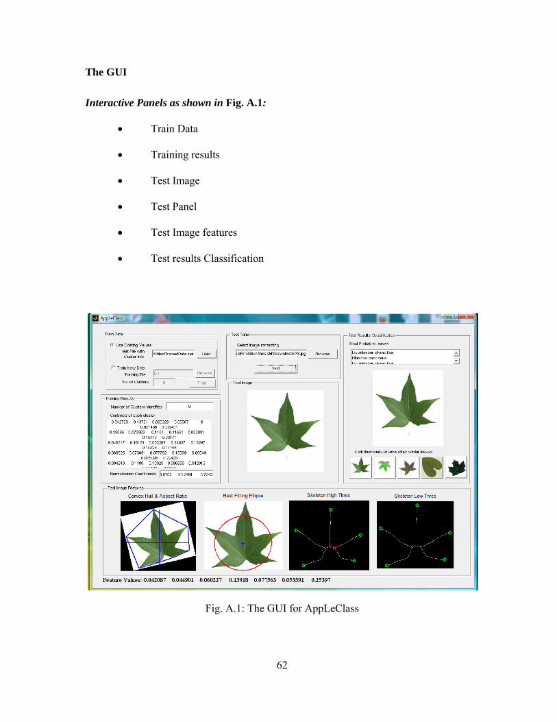
62
The GUI
Interactive Panels as shown in Fig. A.1:
• Train Data
• Training results
• Test Image
• Test Panel
• Test Image features
• Test results Classification
Fig. A.1: The GUI for AppLeClass
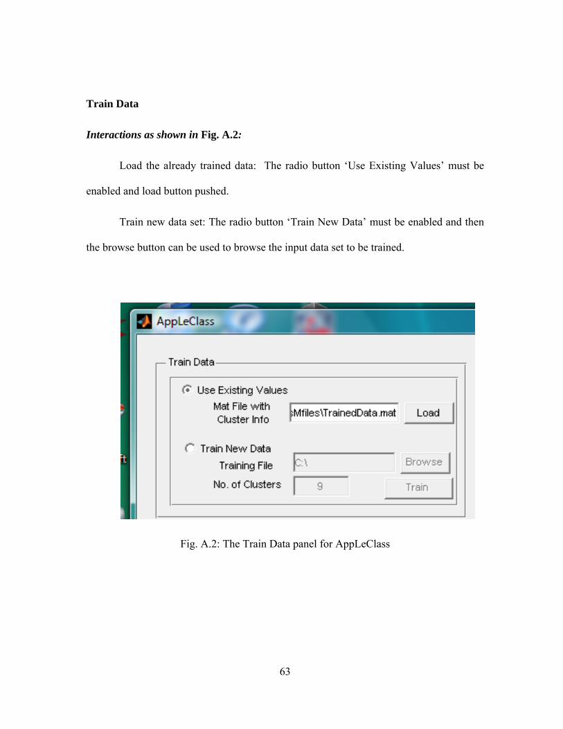
63
Train Data
Interactions as shown in Fig. A.2:
Load the already trained data: The radio button ‘Use Existing Values’ must be
enabled and load button pushed.
Train new data set: The radio button ‘Train New Data’ must be enabled and then
the browse button can be used to browse the input data set to be trained.
Fig. A.2: The Train Data panel for AppLeClass
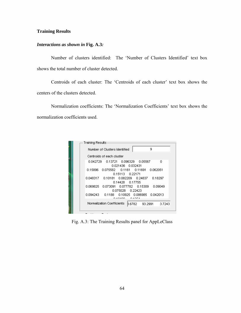
64
Training Results
Interactions as shown in Fig. A.3:
Number of clusters identified: The ‘Number of Clusters Identified’ text box
shows the total number of cluster detected.
Centroids of each cluster: The ‘Centroids of each cluster’ text box shows the
centers of the clusters detected.
Normalization coefficients: The ‘Normalization Coefficients’ text box shows the
normalization coefficients used.
Fig. A.3: The Training Results panel for AppLeClass
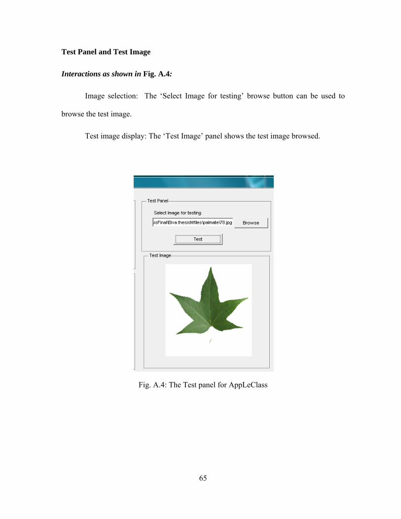
65
Test Panel and Test Image
Interactions as shown in Fig. A.4:
Image selection: The ‘Select Image for testing’ browse button can be used to
browse the test image.
Test image display: The ‘Test Image’ panel shows the test image browsed.
Fig. A.4: The Test panel for AppLeClass
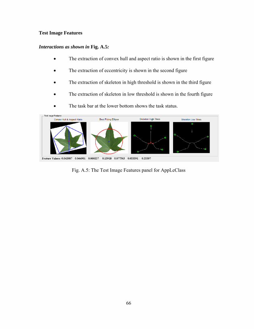
66
Test Image Features
Interactions as shown in Fig. A.5:
• The extraction of convex hull and aspect ratio is shown in the first figure
• The extraction of eccentricity is shown in the second figure
• The extraction of skeleton in high threshold is shown in the third figure
• The extraction of skeleton in low threshold is shown in the fourth figure
• The task bar at the lower bottom shows the task status.
Fig. A.5: The Test Image Features panel for AppLeClass
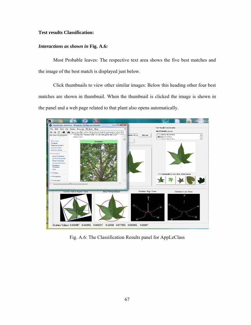
67
Test results Classification:
Interactions as shown in Fig. A.6:
Most Probable leaves: The respective text area shows the five best matches and
the image of the best match is displayed just below.
Click thumbnails to view other similar images: Below this heading other four best
matches are shown in thumbnail. When the thumbnail is clicked the image is shown in
the panel and a web page related to that plant also opens automatically.
Fig. A.6: The Classification Results panel for AppLeClass

68
APPENDIX B
Test Data Set
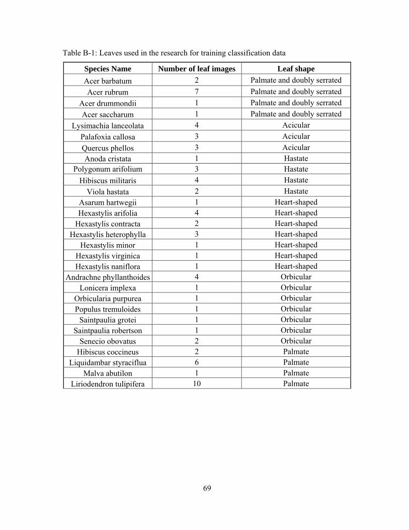
69
Table B-1: Leaves used in the research for training classification data
Species Name Number of leaf images Leaf shape Acer barbatum 2 Palmate and doubly serrated Acer rubrum 7 Palmate and doubly serrated
Acer drummondii 1 Palmate and doubly serrated Acer saccharum 1 Palmate and doubly serrated
Lysimachia lanceolata 4 Acicular Palafoxia callosa 3 Acicular Quercus phellos 3 Acicular Anoda cristata 1 Hastate
Polygonum arifolium 3 Hastate Hibiscus militaris 4 Hastate
Viola hastata 2 Hastate Asarum hartwegii 1 Heart-shaped Hexastylis arifolia 4 Heart-shaped
Hexastylis contracta 2 Heart-shaped Hexastylis heterophylla 3 Heart-shaped
Hexastylis minor 1 Heart-shaped Hexastylis virginica 1 Heart-shaped Hexastylis naniflora 1 Heart-shaped
Andrachne phyllanthoides 4 Orbicular Lonicera implexa 1 Orbicular
Orbicularia purpurea 1 Orbicular Populus tremuloides 1 Orbicular
Saintpaulia grotei 1 Orbicular Saintpaulia robertson 1 Orbicular
Senecio obovatus 2 Orbicular Hibiscus coccineus 2 Palmate
Liquidambar styraciflua 6 Palmate Malva abutilon 1 Palmate
Liriodendron tulipifera 10 Palmate
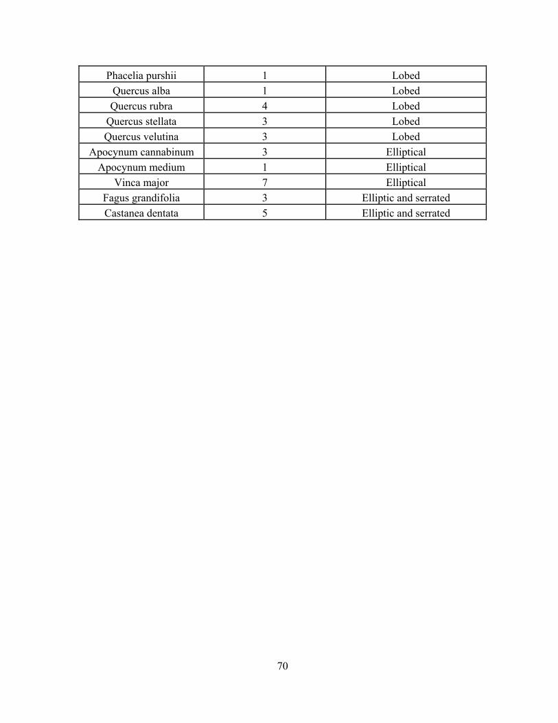
70
Phacelia purshii 1 Lobed Quercus alba 1 Lobed Quercus rubra 4 Lobed
Quercus stellata 3 Lobed Quercus velutina 3 Lobed
Apocynum cannabinum 3 Elliptical Apocynum medium 1 Elliptical
Vinca major 7 Elliptical Fagus grandifolia 3 Elliptic and serrated Castanea dentata 5 Elliptic and serrated

71
APPENDIX C
Sample Images
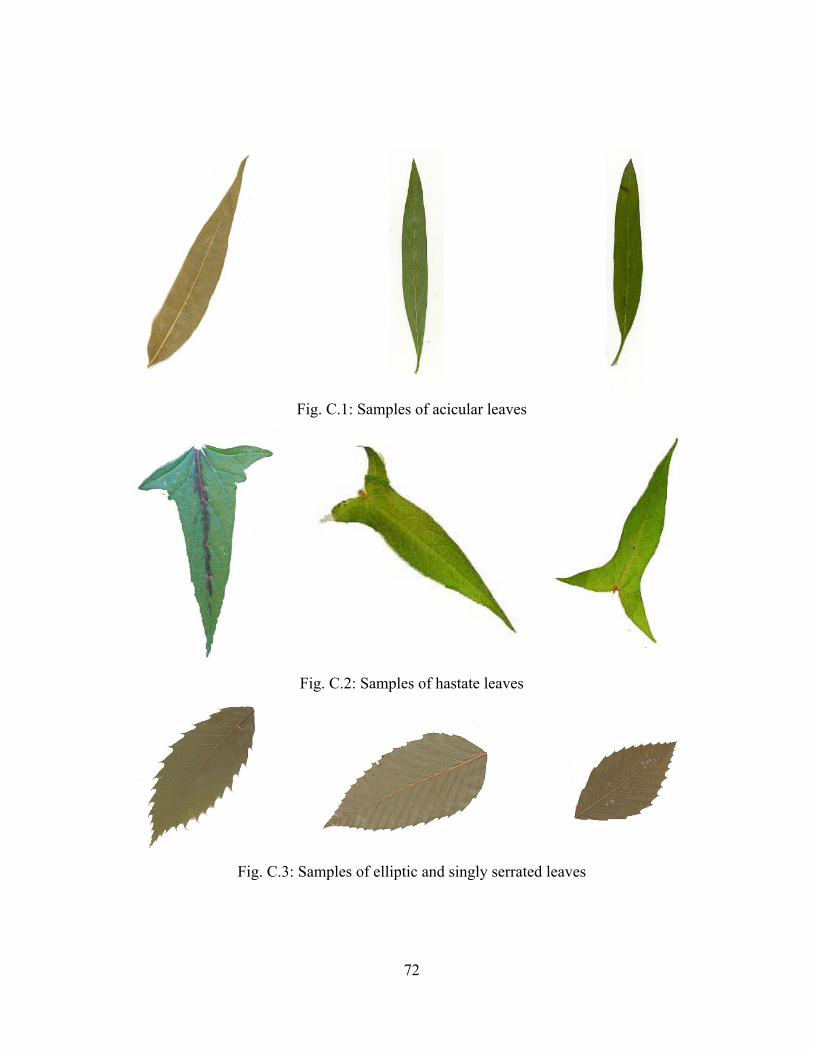
72
Fig. C.1: Samples of acicular leaves
Fig. C.2: Samples of hastate leaves
Fig. C.3: Samples of elliptic and singly serrated leaves
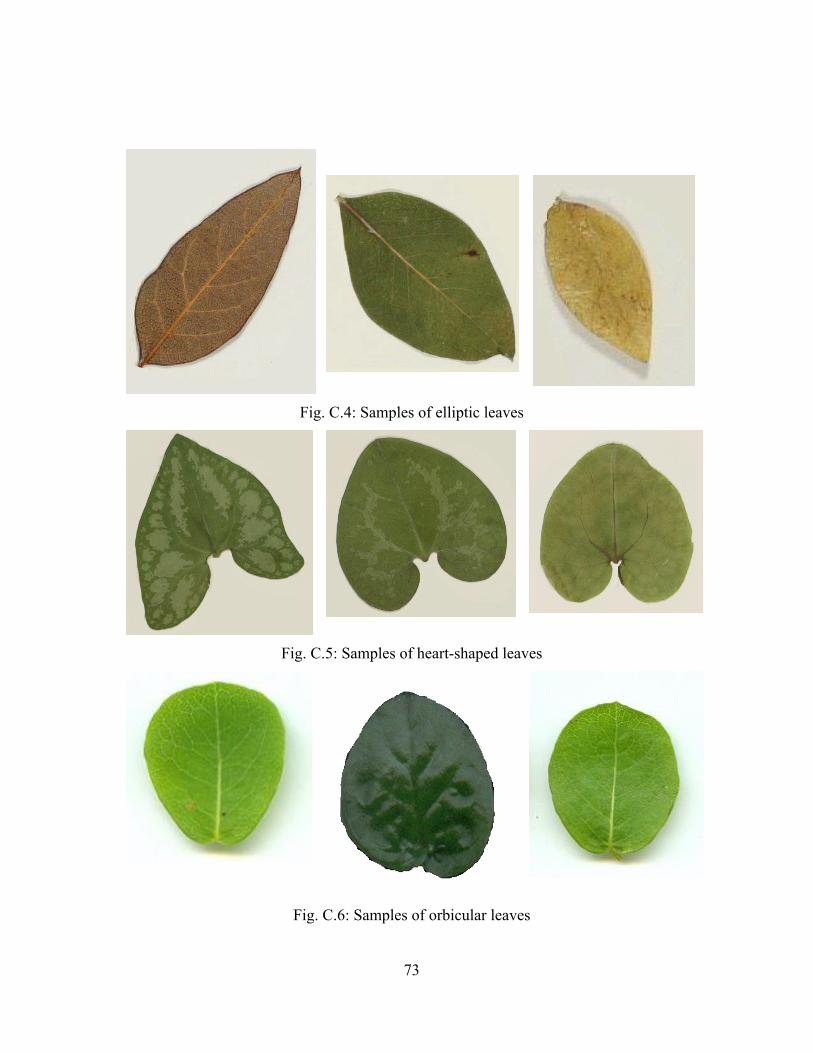
73
Fig. C.4: Samples of elliptic leaves
Fig. C.5: Samples of heart-shaped leaves
Fig. C.6: Samples of orbicular leaves
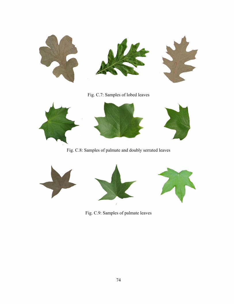
74
Fig. C.7: Samples of lobed leaves
Fig. C.8: Samples of palmate and doubly serrated leaves
Fig. C.9: Samples of palmate leaves
75
VITA
Ms. Biva Shrestha was born in the small city of Biratnagar, Nepal. After finishing
high school in Biratnagar, she moved to the capital city of Nepal, Kathmandu to pursue a
Bachelor’s degree in Computer Engineering. After graduating with a Bachelor of Science
Degree in Computer Engineering from Kathmandu Engineering College-Tribhuwan
University in 2005, she was hired as teaching faculty in the same school for 2 years. In
August 2008, she started her graduate studies at Appalachian State University, Boone, NC,
USA. During the course of her graduate studies at Appalachian State University she was
involved in the Summer Ventures Program in 2009 as a mentor. She will join the Oak Ridge
National Lab Environmental Science Department in Knoxville, Tennessee for a Post Masters
position.