Climate, ecosystem resilience and the slave trade

MPRAMunich Personal RePEc Archive

Climate, ecosystem resilience and theslave trade

James Fenske and Namrata Kala

April 2012

Online at http://mpra.ub.uni-muenchen.de/38398/MPRA Paper No. 38398, posted 27. April 2012 00:38 UTC

http://mpra.ub.uni-muenchen.de/

http://mpra.ub.uni-muenchen.de/38398/

CLIMATE, ECOSYSTEM RESILIENCE AND THE SLAVE TRADE

JAMES FENSKE† AND NAMRATA KALA?

ABSTRACT. African societies exported more slaves in colder years. Lower temperaturesreduced mortality and raised agricultural yields, lowering the cost of supplying slaves.Our results help explain African participation in the slave trade, which is associated withadverse outcomes today. We merge annual data on African temperatures with a panel ofport-level slave exports to show that a typical port exported fewer slaves in a year whenthe local temperature was warmer than normal. This result is strongest where Africanecosystems are least resilient to climate change, and is robust to several alternative spec-ifications and robustness checks. We support our interpretation using evidence from thehistories of Whydah, Benguela, and Mozambique.

1. INTRODUCTION

Africa’s lack of consistent growth has been attributed to many causes, including thecontinent’s geography, its institutions, and its ethnic divisions (Bloom and Sachs, 1998;Collier and Gunning, 1999; Easterly and Levine, 1997). The slave trades, in particular, arecritical to understanding African poverty. Regions of Africa that exported a higher num-ber of slaves suffered selective depopulation (Manning, 1990) and diverted efforts fromproductive activities towards the harvesting of slaves (Whatley and Gillezeau, 2011a).Today, these regions have lower incomes (Nunn, 2008), are less trusting (Nunn andWantchekon, 2010), have more polygamy (Dalton and Leung, 2011), and are more eth-nically divided (Whatley and Gillezeau, 2011b).

Despite the importance of the slave trade, little is known about the influence of Africanfactors on the supply of slaves. Whatley (2008) uses shifts in the demand for slaves toestimate a supply curve in Africa’s guns-for-slaves cycle. His is the only empirical studyof African supply dynamics of which we are aware, and he focuses on demand-side fluc-tuations. Our focus is on supply-side environmental shocks. Historians such as Hartwig(1979), Miller (1982), and Newitt (1995) have suggested that droughts and famines mayhave either increased or decreased the supply of slaves. Crises pushed people to sell

†UNIVERSITY OF OXFORD?YALE UNIVERSITY

E-mail addresses: [email protected], [email protected]: April 26, 2012.We are grateful to Achyuta Adhvaryu, Sonia Bhalotra, Mike Boozer, Rahul Deb, Kenneth Gillingham, Tim-othy Guinnane, Christopher Ksoll, Robert Mendelsohn, Anant Nyshadham, Florian Ploeckl, ChristopherUdry, and the participants of the Yale Environmental Economics seminar for comments.

1

2 JAMES FENSKE AND NAMRATA KALA

themselves or their dependants into slavery, but also led to death and dispersion that re-duced the availability of slaves for export. Lacking consistent data over time and space,these local qualitative studies have been unable to find the net effect of environmen-tal stress on slave supply. We provide the first such results, estimating the impact ofport-specific annual temperature fluctuations on slave exports.

Our approach is to use reconstructed annual data on African temperatures to mea-sure the year-to-year variation in weather conditions over space during the time of thetransatlantic slave trade. We combine this data with port-level annual slave exports. Thepanel nature of this data allows us to control both for port-level heterogeneity and forthe flexible evolution of the slave trade as a whole over time. We find a considerable de-crease in the number of slaves shipped from ports in warmer years. This result is robustto several alternative specifications, including aggregated units of observation, additionof port-specific time trends, and estimation on sub-samples partitioned over time andspace. In addition to studying annual temperatures, we also examine the role of longer-term environmental factors by looking at the effect of climate (that is, long-run trendsin temperature) on slave exports, and find effects that are the same in sign and muchlarger in magnitude.1

Our interpretation is that warmer temperatures led to increased costs of raiding forslaves. These are years of lower productivity for agriculture (Kurukulasuriya and Mendel-sohn, 2006; Lobell and Field, 2007; Tan and Shibasaki, 2003) and of greater mortality(Burgess et al., 2009). In our baseline specification, the magnitude of the impact of a1◦C temperature shock is roughly equal to the mean slave exports from an active port.We argue that this effect worked through higher costs of collecting taxes and tribute forlocal states, lower productivity in supporting sectors of the economy, and higher mortal-ity. We validate our interpretation using case studies of three ports that are influential inour results: Benguela, Whydah, and Mozambique. Our results confirm the importanceof supply-side environmental factors in accounting for the transatlantic slave trade.

We show that the effect we find is stronger in Africa’s sub-humid and dry savannahregions than it is in areas of moist savannah and humid forest. That is, the regions ofAfrica in which agricultural productivity is most sensitive to fluctuations in temperature(Seo et al., 2009) were those that responded most in terms of slave exports. Further, wefind that both long-run trends in climate and short-run shocks around these trends havepower to explain variation in slave exports.

Our results help explain the relationship between the environment and development.Powerful arguments have been advanced linking geography to economic growth (e.g.Bloom and Sachs (1998); Engerman and Sokoloff (1997)). The unchanging nature ofgeographic endowments makes it difficult to separate their direct effects from their in-direct impacts through institutions such as property rights and states (Acemoglu et al.,

1Climate science usually distinguishes between short-run “weather” and long-run “climate.” Climate isa statistical description, usually the mean and variability, of relevant quantities over a period of time. Asdefined by the World Meteorological Organization, this time period is 30 years (IPCC, 2007).

CLIMATE, ECOSYSTEM RESILIENCE AND THE SLAVE TRADE 3

2001; Fenske, 2010). It is also challenging to separate these from the impacts of localunobservable variables that are correlated with geography. Recent work, then, has usednatural experiments such as the eradication of endemic diseases to uncover the bur-dens imposed by geography (Bleakley, 2007; Cutler et al., 2010). Studies that have usedvariation over time in temperature and rainfall have shown that these changes affectdevelopment both over the short run (Dell et al., 2011; Jia, 2011) and over the courseof centuries (Vlassopoulos et al., 2009). The mechanisms for these effects are not yetfully understood. We provide evidence that the impact of temperature shocks on sec-tors outside of agriculture has not been confined to the industrial era, and provide onepossible mechanism by which temperature shocks affect modern incomes. The slavetrade’s effects on modern-day institutions, mistrust and and poverty in Africa are in parta reflection of the continent’s environmental history.

We also add to the existing knowledge on the economics of conflict. Strong correla-tions between economic shocks, economic grievances, and the onset of conflict havebeen asserted in the literature (Collier and Hoeffler, 2004; Miguel et al., 2004), albeitnot without controversy (Ciccone, 2011; Miguel and Satyanath, 2011). The proposedmechanisms for this link focus on the greater relative returns to insurrection over otheractivities and the diminished strength of national militaries during periods of reducedincome (Blattman and Miguel, 2010; Fearon and Laitin, 2003). It is not established thatthe same relationships have held in the past, nor has it been shown whether endemic,parasitic violence will respond in the same way to economic shocks. Violence in Colom-bia intensifies when coca or oil prices rise (Angrist and Kugler, 2008; Dube and Vargas,2008), while Japan’s long recession has cut into the yakuza’s profits from racketeering(Hill, 2006, p. 247). We argue that the returns to the violent harvesting of slaves fell dur-ing depressed periods. To the extent that current economic growth attenuates the riseof conflict (Collier and Hoeffler, 2004), we contribute to the literature that explains howhistory matters for modern conflict.

Finally, we contribute to the literature on the economics of climate change. Exist-ing studies of the importance of historical climate change have focused largely on theimpacts of abrupt and persistent changes on the collapse of civilizations through low-ered agricultural productivity, depopulation, the decline of cities and the weakening ofstates (DeMenocal et al., 2001; Haug et al., 2003; Weiss and Bradley, 2001). We provideevidence that even small, short-run changes had large impacts on the productive sec-tors and coping mechanisms of African societies. As the slave trade shaped institutionsin Africa, these effects will persist into the present.

We proceed as follows. In section 2, we outline our empirical approach and describeour sources of data on temperature shocks and slave exports. In section 3, we provideour baseline results and demonstrate their statistical robustness. We show that that theeffect of temperature differs by agro-ecological zone. We decompose the effect of tem-perature into long-run trends and fluctuations around it. In section 4, we explain the


results. We provide a simple model and argument to account for greater slave exportsduring years of better agricultural productivity and lower mortality. We discuss evidencefrom the secondary literature that connects warmer temperatures to increased mortal-ity and reduced agricultural productivity. We support our interpretation by examiningcase studies of three important slave ports – Whydah, Benguela, and Mozambique. Sec-tion 5 concludes.

2. DATA AND EMPIRICAL STRATEGY

2.1. Empirical strategy. Our data will consist of a panel of annual slave exports andtemperatures for 134 ports that were engaged in the transatlantic slave trade. The de-pendent variable of interest, the number of slaves exported from port i in year t, is cen-sored at 0. Thus, our main specification is the following:

(1) slavesi,t = max(0, α+ β temperaturei,t + δi + ηt + εi,t)

Here, slavesi,t is number of slaves exported from port i in year t. temperaturei,t is thetemperature at port i in year t, δi is a port-level fixed effect, ηt is a year fixed effect andεit is the error term. We estimate (1) using a tobit estimator. Standard errors are clus-tered by the nearest grid point in our temperature data, intersected with year, since thereare fewer grid points than there are ports. In addition to using temperature as the keyexplanatory variable of interest, we also estimate the impacts of the long-run movingaverage (climate) and variation of temperature around this average (climate shocks) onthe supply of slaves.

2.2. Data. In order to estimate (1), we use three principal sources of data. The first cov-ers temperature. The historical data are reported as temperature “anomalies,” and aretaken from Mann et al. (1998a,b). They reconstruct annual temperature anomalies us-ing multivariate calibration on a 5◦ by 5◦ grid. They used a variety of proxy climate indi-cators, combining data from several previous paleoclimatic studies that calculated his-torical temperatures using data from different proxy indicators of temperature. Theseinclude coral, ice cores, tree rings, and other long instrumental records. These anom-alies are reported for each year from 1730 to 1900, and are computed relative to thebaseline average temperature during the period 1902 to 1980. A temperature anomalyof 1◦C at port i in year tmeans that the temperature at iwas 1◦C higher during t than themean temperature at i over the period 1902-1980. We also use a separate temperatureseries from the University of Delaware, which covers the 1902-1980 period. This allows


us to reconstruct the baseline temperatures for each port, permitting us to convert theanomalies into an annual temperature series for each port.2

In addition to using these temperatures directly, we convert them into fluctuationsaround longer-run climate trends by removing the 30-year running mean from eachobservation. These are then treated as shocks over and above the long-term trend inclimate. In our analysis, we also use this running mean of climate as a regressor to es-timate the impact of changes in longer-run climate on the dynamics of the slave trade.Where data are missing on the 5◦ by 5◦ grid, we impute anomalies separately for eachyear using a cubic polynomial in latitude and longitude, with full interactions.

The second source of data that we use is the Trans-Atlantic Slave Trade Database ofEltis et al. (1999).3 The trans-Atlantic slave trade, which is the focus of this study, com-prised roughly 65% of the volume of slaves transported from Africa between 1400 and1900 (Nunn, 2008). Because the temperature data are only available after 1730, we areconfined to analyzing the the impact on the slave trade during this period. Since theoverwhelming bulk of slaves were shipped across the Atlantic in this period, we are ableto study the slave trade when it was at its most active. The database provides voyage-level data on more than 34,000 voyages, including information on the number of slavescarried, the year the ship departed Africa, and the principal port of slave purchase.

We convert these raw data into an annual port-level panel. Since not all ships em-barked from known ports or, in some cases, known regions, this requires assigning sev-eral of the slaves to ports. 60% of slaves come from ports with known latitude-longitudecoordinates. 20% come from a known region (such as the Bight of Benin) but with noport given in the raw data. 20% come from voyages in which only the year is known.4

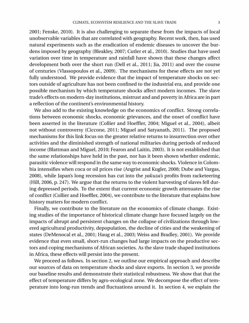
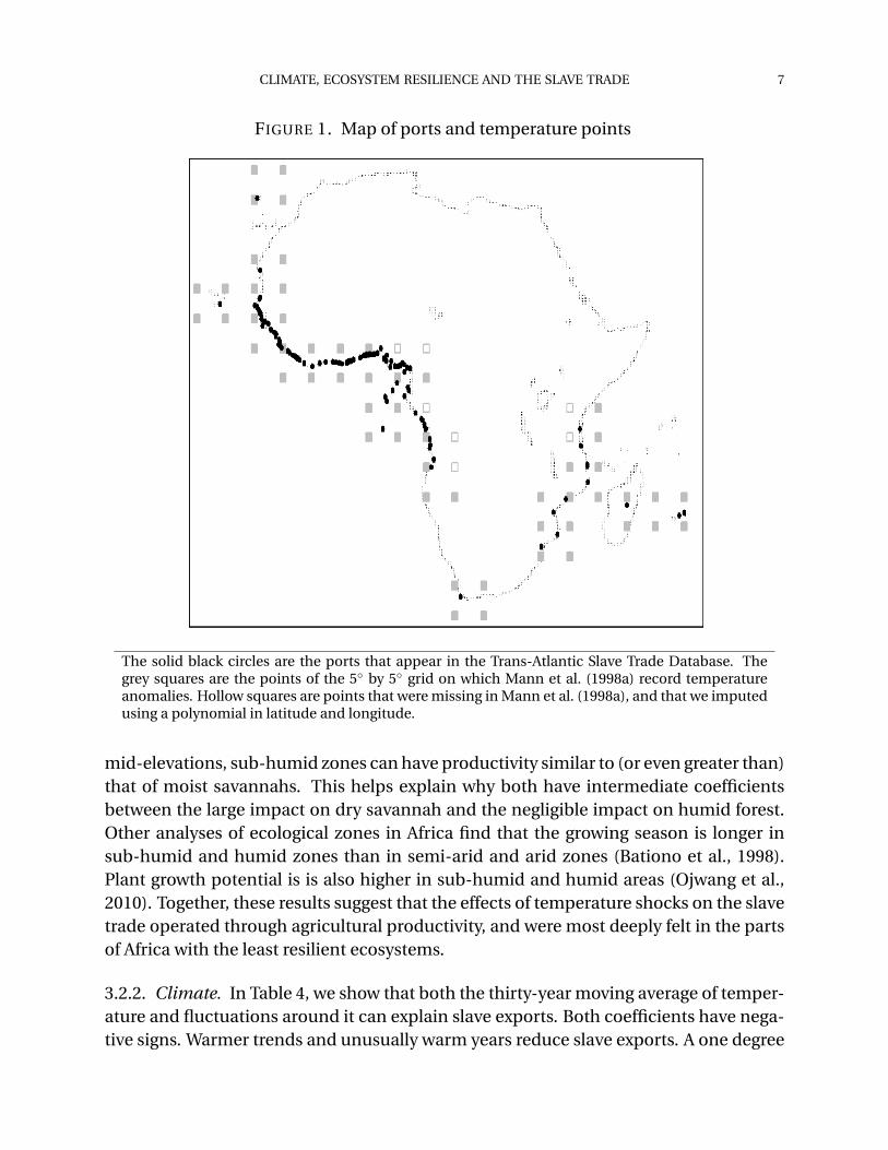
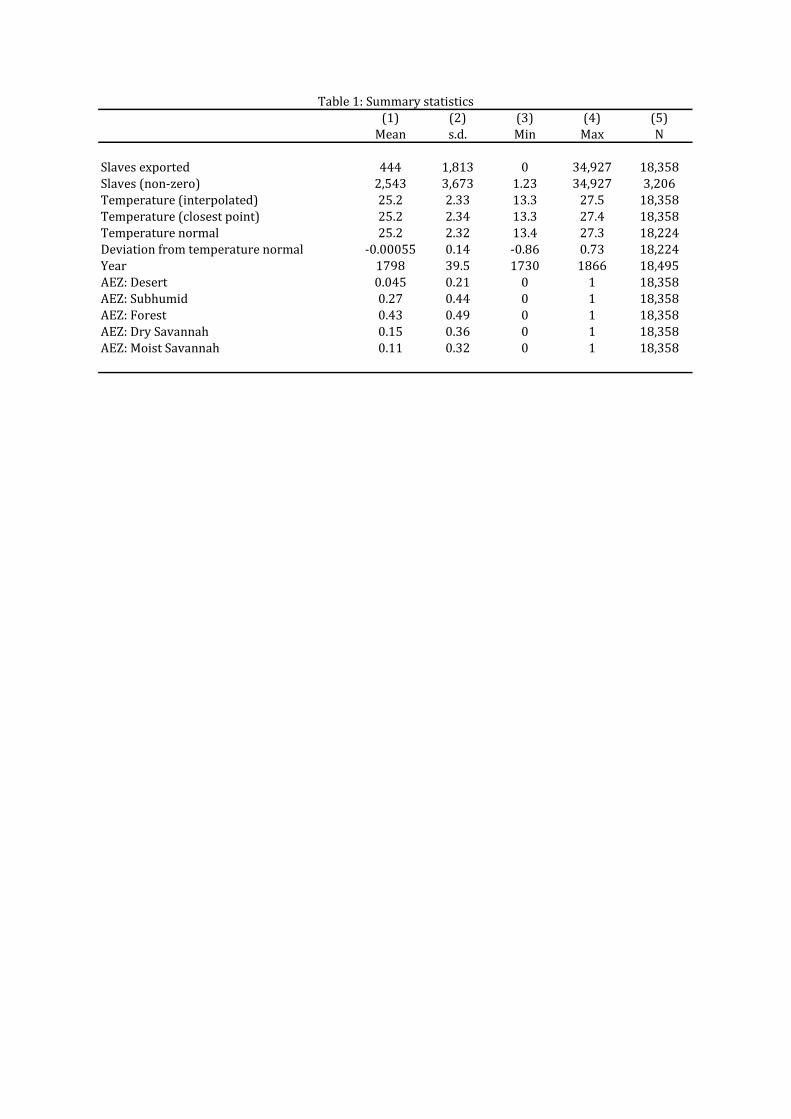
We assign slaves from ships from known regions and unknown ports in proportion tothe number of slaves that are exported from the known ports within that region in agiven year. Analogously, we assign slaves from ships from unknown regions and un-known ports in proportion to the number of slaves that are exported from all knownports within a given year. We obtain a panel of 134 ports spanning 137 years, from 1730to 1866. Temperature shocks for each port are computed by taking the four nearestpoints in the temperature data and interpolating bilinearly. We map both the tempera-ture points for which Mann et al. (1998a) report their data and the ports reported in theTrans-Atlantic Slave Trade Database in Figure 1. Summary statistics for our sample aregiven in Table 1. The mean number of slaves exported annually per port is close to 450,and increases to roughly 2,500 when we only consider ports that exported a non-zero

2Baseline temperatures can be downloaded from http://climate.geog.udel.edu/~climate/html_

pages/download.html#P2009. We originally downloaded the historical anomalies from http://picasso.

ngdc.noaa.gov/paleo/data/mann/. These have since been moved, but we are willing to provide the dataon request.3The database is online, at http://www.slavevoyages.org.4Fewer than 1% of slaves in the data come from ports to which we have been unable to assign geographiccoordinates. We treat these ports as observations with a known region, but no known port.


number of slaves in a given year. The standard deviation reported in the table con-flates differences in temperatures across ports with within-port variation. The standarddeviation of temperature with port means removed is about 0.16. We include a brief de-scription of the impacts of a one standard deviation increase in temperature in section3.

The third source of data is on agro-ecological zones (AEZs). These data classify landinto zones based on climate, elevation, soils and latitude, and are compiled by the Foodand Agriculture Organization (FAO). The original AEZ classification classifies land inAfrica into 16 zones, which includes five climatic zones each at three levels of eleva-tion (high, medium and low), and the desert. These AEZs are stable across time, sincethey are classified using factors such as long-term climate, soil, elevation and latitude.To estimate the effects of temperature separately by AEZ, we collapse the same ecolog-ical zone at each elevation into a single classification. For instance, we classify high-elevation dry savannah, mid-elevation dry savannah and low-elevation dry savannahall as “dry savannah”. Ports are assigned the AEZ of the nearest African administrativeunit in the data used by Kala et al. (2011). The 134 ports in our data comprise desert, drysavannah, moist savannah, sub-humid zone, and humid forest.

3. RESULTS

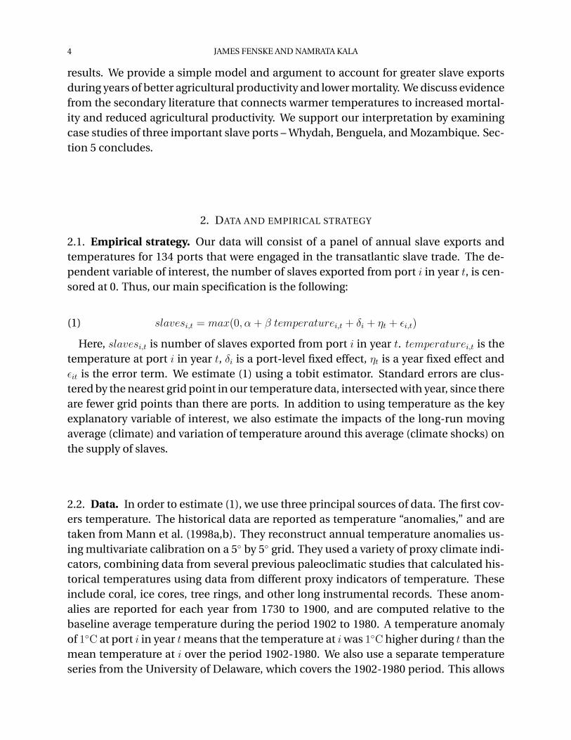
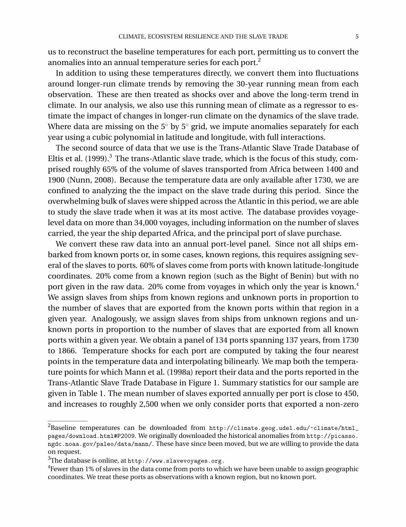
3.1. Main results. We present our main results in Table 2. We find that a one degreeincrease in temperature leads to a one-year drop of roughly 3,000 slaves from each porton average. This is a sizeable effect, roughly equal to the mean for a port whose exportsare nonzero in a given year. For a one standard deviation increase in de-meaned tem-perature (roughly 0.16◦C), the effect would be about 480 slaves.5 This is roughly a onequarter of a standard deviation movement in slave exports.

3.2. Mechanisms.

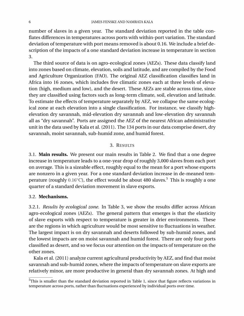
3.2.1. Results by ecological zone. In Table 3, we show the results differ across Africanagro-ecological zones (AEZs). The general pattern that emerges is that the elasticityof slave exports with respect to temperature is greater in drier environments. Theseare the regions in which agriculture would be most sensitive to fluctuations in weather.The largest impact is on dry savannah and deserts followed by sub-humid zones, andthe lowest impacts are on moist savannah and humid forest. There are only four portsclassified as desert, and so we focus our attention on the impacts of temperature on theother zones.

Kala et al. (2011) analyze current agricultural productivity by AEZ, and find that moistsavannah and sub-humid zones, where the impacts of temperature on slave exports arerelatively minor, are more productive in general than dry savannah zones. At high and

5This is smaller than the standard deviation reported in Table 1, since that figure reflects variations intemperature across ports, rather than fluctuations experienced by individual ports over time.


FIGURE 1. Map of ports and temperature points

The solid black circles are the ports that appear in the Trans-Atlantic Slave Trade Database. Thegrey squares are the points of the 5◦ by 5◦ grid on which Mann et al. (1998a) record temperatureanomalies. Hollow squares are points that were missing in Mann et al. (1998a), and that we imputedusing a polynomial in latitude and longitude.

mid-elevations, sub-humid zones can have productivity similar to (or even greater than)that of moist savannahs. This helps explain why both have intermediate coefficientsbetween the large impact on dry savannah and the negligible impact on humid forest.Other analyses of ecological zones in Africa find that the growing season is longer insub-humid and humid zones than in semi-arid and arid zones (Bationo et al., 1998).Plant growth potential is is also higher in sub-humid and humid areas (Ojwang et al.,2010). Together, these results suggest that the effects of temperature shocks on the slavetrade operated through agricultural productivity, and were most deeply felt in the partsof Africa with the least resilient ecosystems.

3.2.2. Climate. In Table 4, we show that both the thirty-year moving average of temper-ature and fluctuations around it can explain slave exports. Both coefficients have nega-tive signs. Warmer trends and unusually warm years reduce slave exports. A one degree


anomaly over the 30-year climate mean has an average impact of nearly 1,300 fewerslave exports per port per year, similar to our main temperature measure, whereas aone degree increase in the 30-year climate mean has an average impact of nearly 18,000fewer slave exports per port per year. The impact of a warm trend is much larger thanan unusually warm single year. A one standard deviation change in within-port climatecauses about 1,800 fewer slaves to be exported per port per year on average.

Part of this difference may be purely mechanical. The within-port variance of thetemperature anomalies is greater than that of the climate anomalies, and the trend forclimate will smooth over year-to-year measurement error in temperature. However,the greater impact of a warming trend is also consistent with the mechanisms throughwhich we argue that environmental factors affected the slave trade. The cumulative im-pact of a warming trend on agricultural productivity and mortality are greater than for asingle warm year. Over time, these will lead to depopulation and out-migration, makingslave exports increasingly unviable. Though societies may adapt to sustained climatechange, a prolonged period of worsening climate can lead to social collapse (DeMeno-cal et al., 2001; Haug et al., 2003).

3.2.3. Other possible mechanisms. Higher temperatures directly reduce agricultural pro-ductivity in Africa. In addition, they predict lower rainfall, which we are unable to ob-serve during the time period covered by our data. Our result, then, mixes the direct im-pact of temperature with indirect effects that operate through rainfall. To establish thesize of the correlation between temperature and rainfall, we use data on temperatureand precipitation from the University of Delaware.6 These report annual temperatureand precipitation figures for points spaced every 0.5 ◦ by 0.5 ◦ from 1900 to the present.We confine our analysis to points in Africa during the years 1900-2000. We regress thelog of annual rainfall on the log of annual temperature, point fixed effects and year fixedeffects. We find that a one percent temperature increase is associated with lower rainfallof 1.26 percent. With a standard error of 0.028, this is very significant. Though this is alarge elasticity, temperature shocks explain less than 1% of the variance in rainfall fluc-tuations.7 While our main result captures the combination of higher temperatures andlower rainfall on the supply of slaves, this suggests that the direct effect of temperatureon agriculture and mortality is what drives our results.8

An alternative reading of our results would infer that higher temperatures were associ-ated with greater natural hazards for transatlantic shippers, and that our results do notreflect “supply side” shocks within Africa. As evidence against this interpretation, we

6These are available at http://climate.geog.udel.edu/~climate/.7That is, regressing the partial residuals from a regression of log rainfall on the point and year fixed ef-fects on the partial residuals from a regression of log temperature on these same fixed effects gives anR-squared of less than 0.01.8We have also performed this same regression using levels, rather than logs, and using binary indicatorsfor whether rainfall or temperature are above their historical means. Both of these give results consistentwith the log specification.


make use of additional data from the Trans-Atlantic Slave Trade Database. For 18,942voyages that have a known year of travel and a known region or port of slave purchase,the data also record whether the journey was completed successfully, failed due to a hu-man hazard, or failed due to a natural hazard. In this sample, we regress the occurrenceof a natural hazard on temperature, port fixed effects, and year fixed effects. To com-pute a temperature for ships without known ports, we assign ships to the modal portin the region of slave purchase. We find that a 1◦C temperature increase reduces theprobability of a natural hazard by 10.4 percentage points, with a standard error of 3.5percentage points. Warmer years were associated with fewer natural hazards for thosewho shipped slaves across the Atlantic. Our main result works in the opposite direction,and overcomes this effect.

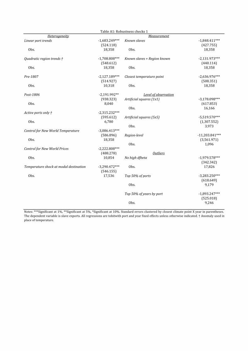
3.3. Robustness. We have tested the robustness of our main result to multiple checksfor unobserved heterogeneity, measurement of slave exports and temperature shocks,the unit of observation, outliers, the estimation method, and the inclusion of lag slaveexports as a control. The results of these tests are presented in the appendix. Notethat, in some specifications, we were unable to compute clustered standard errors usingtemperatures, and so anomalies (with nearly identical point estimates) were used intheir place.

3.3.1. Heterogeneity. To account for port-specific heterogeneity, we have allowed forport-specific linear trends and region-specific quadratic trends.9

We cannot estimate the effect of demand shifts in the slave trade as a whole, sincethese are collinear with the year fixed effects used in our principal specification. Wecan, however, account for port-specific changes in demand by destination region by in-cluding the temperature shock experienced at the nearest new world slave port. Theseports are, as in Nunn (2008), Virginia, Havana, Haiti, Kingston, Dominica, Martinique,Guyana, Salvador, and Rio. Similarly, we show that the results are robust to includingslave prices, both in the embarkation region and in the nearest new world port.10 Alter-natively, we use the disembarkation ports listed in the Trans-Atlantic Slave Trade Data-base to create a modal destination for each African port. Controlling for the anomaly atthese modal destinations also does not change the result.

9Convergence could not be achieved with port-specific quadratic trends using the tobit estimator. If theseare included in an OLS estimation, the impact of temperature on slave exports remains negative andsignificant.10Prices in Africa and the new world are taken from Eltis and Richardson (2004) and cover the years 1671-1810. There are many gaps in these series, especially for the New World ports. These are interpolatedlinearly using the values of the non-missing prices. For example, gaps in the prices of Senegambian slavesare imputed from the prices in the other African regions. The prices in Eltis and Richardson (2004) arereported for five year intervals. We treat prices as constant within these intervals.


3.3.2. Measurement. We show that the method used to assign slaves to ports is not driv-ing the results. We use only the slaves from known ports to calculate port-by-year ex-ports, and achieve similar results to our baseline approach. The effect is smaller, butin proportion to the smaller standard deviation of the dependent variable. The resultsalso survive when using slaves from known ports or regions only. Similarly, we showthat our results are not an artefact of the bilinear interpolation used to construct port-specific temperatures. We can use the temperature calculated from the closest point inthe temperature data and achieve similar results to our baseline.

3.3.3. Level of observation. Our results are not sensitive to the use of ports as the unitof observation. We collapse the African coastline into grid squares one degree in longi-tude by one degree in latitude. We take the sum of all slaves exported from within thatgrid square as slave exports, and the average temperature for ports within that squareas the temperature for that square. The results are very similar to our baseline specifi-cation. Results are similar if they are collapsed into squares five degrees by five degrees.This is equivalent to collapsing to the nearest point in the climate data. Similarly, ifwe collapse slave exports into the major regions of the slave trade (Senegambia, SierraLeone, the Windward Coast, the Gold Coast, the Bight of Benin, the Bight of Biafra, West-Central Africa, and Southeastern Africa), again using the average temperature acrossports within a region to measure the aggregated temperature, we find a large negativeimpact of temperature on slave exports.

3.3.4. Outliers. We discard statistical outliers, re-estimating the results using ordinaryleast squares (OLS), calculating dfbeta statistics, and then re-estimating the main tobitspecification without observations whose absolute dfbeta is greater than 2/

√N .11 Simi-

larly, we show that we can achieve our main results without relying on certain subsets ofthe data. We eliminate the smaller ports in the sample by removing the bottom 50% ofports by total number of slaves exported. We also show that the results are not driven byinactive ports by excluding all observations from the data where a port has either ceasedto export slaves, or has not yet begun its participation in the trade.

The results are not driven by any one region within Africa. We drop these regions oneat a time. Though the effect is clearly largest for West-Central Africa, this can in partbe accounted for by the region’s overwhelming preponderance in the slave trade. Nunn(2008) estimates that Angola alone sent more than three and a half million slaves acrossthe Atlantic.

3.3.5. Estimator. We employ several alternative estimation strategies. We begin by re-estimating the main equation using OLS. The effect of a temperature shock remainsnegative and significant. Unsurprisingly, the estimated effect is smaller if we do not

11The standard test of discarding high-leverage observations is not reported. Since no observations haveleverage greater than 2(df + 1)/N , these results are identical to the main specification.


account for censoring. We also find a significant and negative effect of temperature us-ing a binary indicator for nonzero slave exports as the dependent variable, discardingobservations with no slave exports, taking first-differences, or including lagged tem-perature as a control. The number of observations is large relative to the number offixed effects, and so the incidental parameters problem should only be a minor con-cern. However, because (1) is non-linear, Wooldridge (2002, p. 542) suggests includingport-specific mean temperatures temperaturei rather than port fixed effects. Under theassumption that the port fixed effects δi are linearly related to the port-specific means(δi = ψ + ai + λtemperaturei), this will give consistent estimates of β. The results arecongruent with our baseline specification.

3.3.6. Inclusion of lag slave exports. We include lagged slave exports as a control. Sinceslave exports in the previous year are correlated with the error term, we use the dif-ference between slaves exported two years ago and slaves exported three years ago asan instrumental variable for lagged slave exports. Although the coefficient estimate issmaller than in the baseline, the results again suggest a sizable reduction in slave ex-ports during warmer years. Roughly 1,900 fewer slaves are exported per port in a yearwith a 1◦C rise in temperature.

Wooldridge (2005) suggests that censored models with a lagged dependent variablesuch as ours can be estimated by including lagged slave exports, mean temperature, andinitial slave exports in the estimation. This is consistent under the assumption that theport-level fixed effects δi can be decomposed into δi = ψ+ai+λ1slavesi0+γtemperaturei.This decomposition assumes a relationship between the initial number of slaves fromwhen the trade first started and the port-fixed characteristics and reduces it to a regulartobit estimation. Here too, warmer temperatures predict a sizeable reduction in slaveexports, about 1,300 slaves per port in a year with a 1◦C temperature shock.

Re-estimating the same specification using the Arellano-Bond estimator (using twolags as an instrument), we find that the estimated coefficient on temperature is verysimilar to the estimate obtained using OLS. This is larger than the coefficient obtainedby including the lagged dependent variable and estimating the effect using OLS. Thissuggests that, if there is any bias on the estimated coefficient on temperature when in-cluding the un-instrumented lag, it is towards zero, understating the effect of tempera-ture on slave supply.

4. INTERPRETATION

4.1. Argument. We argue that higher temperatures raised the cost of slave capture andexport. Consider a coastal African ruler who maximizes profits from selling slaves, as inFenoaltea (1999). The ruler is a price taker, and traders at the coast will pay p per slave.The ruler “produces” a quantity S of slaves using an army that he controls. The costof raiding for S slaves is C(S, T ), where T is temperature. Costs are convex in both thequantity of slaves exported and in temperature. That is, CS > 0, CSS > 0, CT > 0, and


CST > 0. The ruler, then, will choose S to maximize pS − C(S, T ). Temperature, then,reduces exports:

dS

dT= −CST

CSS

< 0.

The critical assumption is that CST > 0. We believe this for four reasons. First, theruler’s costs of extracting tribute in order to feed a slave-harvesting army rise during badharvests. Second, the mortality of slaves, soldiers and porters will rise in warmer years.Third, higher temperatures lead to greater evapotranspiration, increasing the probabil-ity that drought will set in. Areas of slave supply become more disordered, raising thecosts of raiding directly. Finally, the slave trade depended on complementary economicactivities that provisioned ships, fed the populations of the ports, and supplementedthe incomes of slave traders.

4.2. Temperature, agriculture, and mortality. There is substantial evidence that tem-perature shocks affect agriculture and mortality in the present. Studies of the impactof climate on modern agricultural productivity in Africa (Kala et al., 2011; Kurukula-suriya and Mendelsohn, 2006) indicate that higher temperatures relative to the base-line climate have a negative impact on productivity, particularly for non-irrigated agri-culture. In addition, higher temperatures increase evapotranspiration (Brinkman andSombroek, 1996). This indicates that colder years lead to a relatively higher level of wa-ter availability for plants, which is crucial in certain stages of plant growth. Other stud-ies of temperature impacts on the productivity of tropical agriculture find similar results(Guiteras, 2009; Sanghi and Mendelsohn, 2008) Thus, the link between colder years andhigher agricultural productivity in the tropics is well established.

There is also evidence that higher temperatures increase disease burdens that raisemortality (Burgess et al., 2009). Studies of the relationship between disease and temper-ature find that higher temperatures are more conducive to the spread and transmissionof diseases such as malaria and yellow fever (Alsop, 2007). Malaria and yellow fever haveplaced a particularly heavy mortality burden on Africa throughout the continent’s his-tory (Gallup and Sachs, 2001; Ngalamulume, 2004). Further, arid AEZs and modern-daychild malnutrition are positively correlated (Sharma et al., 1996).

4.3. Case studies. In this section, we show that the histories of three major slave ports– Benguela, Whydah, and Mozambique – are consistent with our interpretation of ourempirical findings. These three cases are selected as statistically influential ports thatare well documented in the secondary literature and that come from three separate re-gions of the slave trade. We show that, in each case, the slave trade was dependent onthe health of the local agrarian economy.

4.3.1. Benguela. Benguela, in southern Angola, was founded in 1617 (Candido, 2006,p. 4). The town began its involvement in the slave trade by shipping slaves to Luanda for


re-export (Candido, 2006, p. 4). After 1716, the legal requirement that ships sail to Lu-anda before leaving Angola was removed, and Benguela grew beyond the supervision ofthe Portuguese administration centered at Luanda (Candido, 2006, p. 22). Between 1695and 1850, Candido (2006, p. 18) estimates that Benguela shipped nearly half a millionslaves to the new world, making it the fourth most important port in the transatlantictrade, behind Luanda, Whydah, and Bonny. Though most of the slaves shipped throughBenguela were Ovimbundu from the Western slopes of the highlands directly east of thetown (Curtin and Vansina, 1964, p. 189), these slaves were sold through a commercialnetwork integrated with the one that served Luanda (Miller, 1989, p. 383).

War, abduction, tribute, debt, judicial enslavement, pawnship, sale of relatives, andself-enslavement were all important sources of the slaves sold at Benguela (Candido,2006, p. 48). Warfare between local societies was seen as a legitimate method of en-slavement, though this was difficult to distinguish from “illegal” methods such as kid-napping, which became more prevalent due to rising prices during the 1830s (Candido,2006, p. 80). Judicial enslavement, similarly, only became a major source of captives inthe mid-nineteenth century (Candido, 2006, p. 66).

Miller (1982, p. 29-30) argues that droughts, famines, and epidemics served to in-crease the supply of slaves from West-Central Africa through self-enslavement and aflow of refugees. We find, however, that slave exports are negatively correlated with ad-verse temperature shocks. There are two principal mechanisms for this in the case ofBenguela. First, bad harvests created political disorder. Second, they disturbed activi-ties complementary to the slave trade.

In West-Central Africa, droughts led to “violence, demographic dispersal, and emigra-tion” (Miller, 1982, p. 32). Major confrontation between Portuguese forces and Africanstates occurred with “suspicious regularity at the end of periods of significantly reducedprecipitation” (Miller, 1982, p. 24). Tribute from local Sobas was often rendered in theform of slaves (Candido, 2006, p. 24), and disruption to this political order would haveconstricted the flow of slaves. Raids and famines both pushed Africans to resettle inmore distant regions (Candido, 2006, p. 48), raising the costs of capture.

The slave trade depended on the health of the local economy. African products, espe-cially palm-cloth and salt, figured largely in the eighteenth century Angolan slave trade(Klein, 1972, p. 910). Portuguese soldiers in the interior were often without a regularsalary, and so exchanged gunpowder inland for chickens and other agricultural prod-ucts (Candido, 2006, p. 38). Military officials, similarly, had to buy food and other com-modities using trade goods such as beads and textiles (Candido, 2006, p. 112). In ad-dition to slaves, cattle, salt, ivory and shells were shipped from Benguela to Luanda inreturn for cassava flour. These were used to buy slaves and to supply ships (Candido,2006, p. 24). Slaves held inland at Cacinda worked in agriculture to feed themselves andpassing slave coffles. Their produce was also sent directly to Benguela (Candido, 2006,p. 213).


Luso-African traders working in the interior engaged directly in slave raids (Candido,2006, p. 83). After the 1820s, slave exporters diversified increasingly into so-called “le-gitimate” goods (Candido, 2006, p. 112). Slaves were marched to the coast by caravan,and caravan porters used these as opportunities to trade on their own accounts (Can-dido, 2006, p. 124). Periods of higher temperatures, in addition to providing fewer tradeopportunities, would have been times of greater mortality for both slaves and porters.

4.3.2. Whydah. Whydah (or Ouidah), in southern Benin, was founded before the be-ginnings of European trade there in the seventeenth century (Law, 2004, p. 25). Thetown was brought under the control of Dahomey between 1727 and 1733, after whichthe volume of slaves exported declined (Law, 2004, p. 52-59). Despite the town’s pecu-liar position 4 km inland, Whydah was Dahomey’s principal port. It remained an im-portant point of slave embarkation throughout the trade. Exports were between 8,000and 9,000 persons annually during the 1750s, and some 4,500 per year circa 1788 (Law,2004, p. 125-126). In the late 1700s, these were shipped mostly to Brazil and the FrenchCaribbean (Law, 2004, p. 126).

The two principal sources of slaves traded through Whydah during the time period ofthis study were capture by the Dahomean army and purchase from the interior (Law,2004, p. 138). Whydah fits the model closely, as the supply of slaves depended greatlyon the local state’s military strength. Dahomey competed with other states of the “SlaveCoast” to supply slaves for the Atlantic trade. With the rise of Oyo in the late seventeenthcentury, the share of slaves shipped by Dahomey, and hence through Whydah, declined(Law, 2004, p. 126). Oyo attacks had made passage through Dahomey dangerous forslave suppliers (Ross, 1987, p. 369). After Dahomey’s victory over Oyo in the early 1820s,she was free to launch campaigns in the Mahi and Yoruba countries to the north-eastthat increased slave exports through Whydah (Curtin and Vansina (1964, p. 190), Law(2004, p. 160)). During the 1750s, the king of Dahomey attempted to forcibly unify theMahi polities in order to facilitate trade through the region (Law, 1989, p. 53). The Da-homean capture of Whydah itself appears to have been motivated by the state’s desireto gain better access to the slave trade, and as its involvement grew the state becamemore militarized (Law, 1986, p. 247,258).

The early literature on Dahomey supposed, wrongly, that the slave trade was a royalmonopoly. While this was not the case, captives brought by the king’s army formeda substantial part of the trade (Law, 2004, p. 111). The state also enjoyed many specialprivileges, such as regulation of prices and the right to sell slaves first (Law, 2004, p. 129).Private middlemen supplemented this royal trade by purchasing them from neighbor-ing countries (Law, 2004, p. 111). They became especially important once Dahomeybecame a significant port in the 1750s and 1760s (Law, 1989, p. 59). The ability to ac-quire slaves was tied to conditions in regions of slave supply; in the 1770s and 1780s,for example, disturbances on the coast made it difficult for Dahomey to buy slaves ineastern markets (Ross, 1987, p. 370).


This middleman trade also depended on the strength of the Dahomean army. It wasthe Dahomean conquest of alternative ports such as Jaquin and Apa that drove tradetowards Whydah (Ross, 1987, p. 361). Strict military control over the movements of Eu-ropean traders living at Whydah kept the trade in Dahomean hands (Ross, 1987, p. 367).Though Dahomey abandoned its attempts to monopolize the trade of the slave coastafter roughly 1750, it continued to attract trade by offering suppliers safer routes thanthrough the surrounding country (Ross, 1987, p. 369).

The slave trade at Whydah did not exist separately from the local economy. The slavetrade was supported by the local retail trade, agriculture, fishing and salt-making (Law,2004, p. 77). Though Whydah’s trade consisted mostly of slaves, other goods such asivory, cotton, cloth and palm oil were also exported from the port (Law, 2004, p. 125).The city depended on goods imported from the interior that were consumed locally,including kola from Asante and natron from Borno (Law, 2004, p. 83). The earningsof private merchants were spent locally, while the trade itself depended on the labourof local porters, water-rollers, and laundry women, among other workers (Law, 2004,p. 147). Markets at Whydah sold a mix of local products and imported goods (Law, 2004,p. 148).

Because Europeans extended credit in the form of goods in return for the promisethat slaves would be delivered at a future date, the trade depended on the conditions en-countered by local merchants (Law, 2004, p. 133). Even before the Dahomean capture ofWhydah, supply-side factors constrained the growth of slave exports. Law (1994, p. 82)reports that demand outpaced the Allada capacity to supply slaves in the 1630s, 1640sand 1670s, leading local merchants to become increasingly indebted to their Dutch buy-ers.

4.3.3. Mozambique. Though the Portuguese established a fort on Mozambique Islandin 1508, the slave trade developed slowly in southeastern Africa due to the greater voy-age lengths involved (Klein, 2010, p. 69). In the 1600s, Mozambique Island traded mostlyin ivory (Newitt, 1995, p. 177). Mixed-race Afro-Portuguese settlers dominated tradealong the Zambezi river until the nineteenth century, creating estates that functioned asminiature states complete with slave armies (Klein, 2010, p. 70). The slave trade that be-gan to take off after 1750 was initially in French hands, and accelerated from the 1770s(Newitt, 1995, p. 245-6). Though interrupted by the Napoleonic Wars, the slave tradeshowed an upward trend until the 1830s. In the nineteenth century, Brazilian and Arabtraders came to overshadow the French (Alpers, 1970, p. 84). There were four distinctmarkets for Mozambican slaves: French islands in the Indian Ocean, the Americas, thePortuguese East African possessions, and Madagascar (Newitt, 1972, p. 659).

Africans in the interior typically acquired female slaves through capture or purchase,while males were obtained through clientship arrangements that traded labor servicefor cattle or wives (Newitt, 1995, p. 234). Slaves exported from Mozambique were gen-erated mostly among the Makua (Newitt, 1995, p. 247). Little is known about how this


increased supply was provided. The only detailed contemporary account notes that car-avans with trade goods would pass between settlements until a local chief was able tosupply slaves. At that point, they would stop to establish a market (Newitt, 1995, p. 252).

Newitt (1995, p. 244) believes that it was the famines of the early nineteenth centurythat helped fill the slavers’ barracoons. His argument focuses on the severe droughtsthat occurred from 1794 to 1802 and from 1823 to the late 1830s that are collectively re-ferred to as the mahlatule. Local people normally responded to dry periods by intensify-ing other income-generating activities, such as hunting, gold mining and trading. Whenthese too failed, they turned to out-migration, which led to instability, war, banditry andslaving (Newitt, 1995, p. 253). The long second drought upended peasant life, and muchof the population starved, died of smallpox or moved elsewhere (Newitt, 1995, p. 254).The power of both the Afro-Portuguese and local African chieftaincies was undermined(Newitt, 1995, p. 254-55). Klein (2010, p. 71) expresses a similar view.

There are two problems with Newitt’s (1995) interpretation. First, there is no controlgroup. The first half of the nineteenth century was also a period of sustained Brazil-ian demand for slaves and British patrols that pushed trade towards West-Central andSoutheastern Africa. Newitt does not test whether Mozambique exported more slavesduring the mahlatule than would be expected given demand conditions. After 1811,Portugal allowed Brazilian ships to trade freely with its East African ports, reinforcingthis greater demand (Klein, 2010, p. 72). Second, while drought produced disorder inSoutheast Africa, it is not evident that this facilitated the supply of slaves. By disrupt-ing settlement patterns, trading networks, and local states, droughts may have actedjust as strongly to raise the costs of slaving. The Nguni states that were pushed northof the Zambezi by the mahlatule were known for their fierceness and economic self-sufficiency, both of which isolated the region from outside trade (Newitt, 1995, p. 264).The droughts similarly slowed Portuguese movement into the interior, and expansionby Afro-Portuguese along the Zambezi was only restored as peace returned in the 1850sand 1860s (Newitt, 1995, p. 264, 284). In addition, drought directly raised transportationcosts by making rivers impassable (Newitt, 1995, p. 255).

As a military fortification, the island was dependent for its food from the mainlandand neighboring islands (Newitt, 1995, p. 190). The island was often short on provisions(Alpers, 1970, p. 94). Ships engaging in the slave trade were similarly dependent on foodand other supplies from local sources (Newitt, 1995, p. 249). French traders who visitedthe island also traded in rice, meat and cattle (Alpers, 1970, p. 94). These needs werekeenly felt in periods of bad weather; the island was forced to import food during thedrought in 1831 (Alpers, 2001, p. 77). As in the other cases studied, the functioning ofthe slave trade at Mozambique depended on complementary activities in the interior.


5. CONCLUSION

We find that environmental shocks within Africa influenced the dynamics of the slavetrade. The effects we find are large. A temperature increase of one degree Celsius re-duced annual exports by roughly 3,000 slaves per port. We interpret these as shifts inthe cost of slave supply, operating through mortality and the productivity of comple-mentary sectors. The histories of Benguela, Whydah, and Mozambique support ourinterpretation.

We have advanced the existing understanding of Africa’s participation in the slavetrade by incorporating previously unutilized, time-varying measures of weather shocksspanning all sending regions. This exercise demonstrates the importance of supply-sidefactors in the dynamics of the transatlantic slave trade. This has also enabled us to pro-vide new evidence on the channels through which geography shapes economic devel-opment in a historical setting. We are able to examine the responsiveness of a differentform of conflict to economic shocks than is typically studied in the literature. Ratherthan being encouraged by economic distress, slave raiding was hindered by it.

There are, of course, limitations of our approach. Data availability prevent us to fromlooking at the dynamics of the Indian Ocean, Red Sea, or internal African slave trades.Similarly, we are unable to examine the period before 1730, or environmental factorsother than temperature. Further, our results should not be over-interpreted; we cansay little about the relative importance of the proposed mechanisms through which thelink between temperature and the slave trade worked. Depending on their resource en-dowments and institutions, societies may adapt to change, particularly to slow-movingchanges in climate. As climate scientists advance in their reconstruction of the environ-mental past, we are hopeful that it will become possible to examine further these issuesand to better understand the long-run causes of Africa’s poverty.

REFERENCES

Acemoglu, D., Johnson, S., and Robinson, J. (2001). The colonial origins of comparativedevelopment: An empirical investigation. American Economic Review, pages 1369–1401.

Alpers, E. (1970). The French slave trade in East Africa (1721-1810). Cahiers d’etudesafricaines, 10(37):80–124.

Alpers, E. (2001). A complex relationship: Mozambique and the Comoro Islands in the19th and 20th centuries. Cahiers d’etudes africaines, 41(161):73–95.

Alsop, Z. (2007). Malaria returns to Kenya’s highlands as temperatures rise. The Lancet,370(9591):925–926.

Angrist, J. and Kugler, A. (2008). Rural windfall or a new resource curse? Coca, income,and civil conflict in Colombia. The Review of Economics and Statistics, 90(2):191–215.

Bationo, A., Lompo, F., and Koala, S. (1998). Research on nutrient flows and balances inWest Africa: state-of-the-art. Agriculture, ecosystems & environment, 71(1-3):19–35.


Blattman, C. and Miguel, E. (2010). Civil war. Journal of Economic Literature, 48(1):3–57.Bleakley, H. (2007). Disease and development: Evidence from hookworm eradication in

the American South. Quarterly Journal of Economics, 122(1):73–117.Bloom, D. and Sachs, J. (1998). Geography, demography, and economic growth in Africa.

Brookings papers on economic activity, 1998(2):207–295.Brinkman, R. and Sombroek, W. (1996). The effects of global change on soil conditions in

relation to plant growth and food production. Global Climate Change and AgriculturalProduction, pages 49–63.

Burgess, R., Deschenes, O., Donaldson, D., and Greenstone, M. (2009). Weather anddeath in India. MIT Working paper.

Candido, M. (2006). Enslaving frontiers: slavery, trade and identity in Benguela, 1780-1850. PhD Thesis, York University (Canada).

Ciccone, A. (2011). Economic shocks and civil conflict: A comment. American EconomicJournal: Applied Economics, 3(4):215–227.

Collier, P. and Gunning, J. (1999). Explaining African economic performance. Journal ofeconomic Literature, 37(1):64–111.

Collier, P. and Hoeffler, A. (2004). Greed and grievance in civil war. Oxford economicpapers, 56(4):563–595.

Curtin, P. and Vansina, J. (1964). Sources of the nineteenth century Atlantic slave trade.The Journal of African History, 5(02):185–208.

Cutler, D., Fung, W., Kremer, M., Singhal, M., and Vogl, T. (2010). Early-life malaria ex-posure and adult outcomes: Evidence from malaria eradication in India. AmericanEconomic Journal: Applied Economics, 2(2):72–94.

Dalton, J. and Leung, T. (2011). Why is polygyny more prevalent in Western Africa? AnAfrican slave trade perspective. Working paper.

Dell, M., Jones, B., and Olken, B. (2011). Climate shocks and economic growth: Evidencefrom the last half century. NBER Working Paper, 14132.

DeMenocal, P. et al. (2001). Cultural responses to climate change during the lateHolocene. Science, 292(5517):667.

Dube, O. and Vargas, J. (2008). Commodity price shocks and civil conflict: Evidencefrom Colombia. manuscript, Harvard University.

Easterly, W. and Levine, R. (1997). Africa’s growth tragedy: Policies and ethnic divisions.Quarterly journal of Economics, 112(4):1203–1250.

Eltis, D., Behrendt, S. D., Richardson, D., and Klein, H. S. (1999). The trans-Atlantic slavetrade: a database on CD-ROM. Cambridge University Press.

Eltis, D. and Richardson, D. (2004). Prices of African slaves newly arrived in the Amer-icas, 1673-1865: New evidence on long-run trends and regional differentials. Slaveryin the Development of the Americas, pages 181–218.

Engerman, S. L. and Sokoloff, K. L. (1997). Factor endowments, institutions, and differen-tial paths of growth among new world economies, pages 260–304. How Latin America


Fell Behind. Essays on the Economic Histories of Brazil and Mexico, 1800-1914. Stan-ford University Press.

Fearon, J. and Laitin, D. (2003). Ethnicity, insurgency, and civil war. American PoliticalScience Review, 97(1):75–90.

Fenoaltea, S. (1999). Europe in the African mirror: the slave trade and the rise of feudal-ism. Rivista di storia economica, 15(2):123–166.

Fenske, J. (2010). Ecology, trade and states in pre-colonial Africa. Working Paper.Gallup, J. and Sachs, J. (2001). The economic burden of malaria. The American journal

of tropical medicine and hygiene, 64(1 suppl):85–96.Guiteras, R. (2009). The impact of climate change on Indian agriculture. Manuscript,

Department of Economics, University of Maryland, College Park, Maryland.Hartwig, G. (1979). Demographic considerations in East Africa during the nineteenth

century. The International Journal of African Historical Studies, 12(4):653–672.Haug, G., Gunther, D., Peterson, L., Sigman, D., Hughen, K., and Aeschlimann, B. (2003).

Climate and the collapse of Maya civilization. Science, 299(5613):1731.Hill, P. (2006). The Japanese mafia: yakuza, law, and the state. Oxford University Press,

USA.IPCC (2007). Climate change 2007: The physical science basis. contribution of working

group i to the fourth assessment report of the intergovernmental panel on climatechange. Solomon, S., D. Qin, M. Manning, Z. Chen, M. Marquis, K.B. Averyt, M.Tignorand H.L. Miller (eds.). Cambridge University Press, Cambridge, United Kingdom andNew York, NY, USA.

Jia, R. (2011). Weather shocks, sweet potatoes and peasant revolts in historical China.HiCN Working Papers.

Kala, N., Kurukulasuriya, P., and Mendelsohn, R. (2011). The impact of climate changeon agro-ecological zones: Evidence from Africa. Working Paper.

Klein, H. (1972). The portuguese slave trade from Angola in the eighteenth century. TheJournal of Economic History, 32(4):894–918.

Klein, H. (2010). The Atlantic slave trade. Cambridge Univ Pr.Kurukulasuriya, P. and Mendelsohn, R. (2006). A Ricardian analysis of the impact of cli-

mate change on African cropland. World Bank Research Policy Working Paper (forth-coming).

Law, R. (1986). Dahomey and the slave trade: Reflections on the historiography of therise of Dahomey. The Journal of African History, 27(02):237–267.

Law, R. (1989). Slave-raiders and middlemen, monopolists and free-traders: The supplyof slaves for the Atlantic trade in Dahomey c 1715-1850. Journal of African history,30:45–68.

Law, R. (1994). The slave trade in seventeenth-century Allada: a revision. African eco-nomic history, (22):59–92.


Law, R. (2004). Ouidah: the social history of a West African slaving ‘port’, 1727-1892.James Currey.

Lobell, D. and Field, C. (2007). Global scale climate–crop yield relationships and theimpacts of recent warming. Environmental Research Letters, 2:014002.

Mann, M., Bradley, R., and Hughes, M. (1998a). Global-scale temperature patterns andclimate forcing over the past six centuries. Nature, 392(6678):779–787.

Mann, M., Bradley, R., and Hughes, M. (1998b). Global six century temperature patterns.IGBP PAGES World Data Center.

Manning, P. (1990). Slavery and African Life: occidental, oriental, and African slavetrades, volume 67. Cambridge Univ Pr.

Miguel, E. and Satyanath, S. (2011). Re-examining economic shocks and civil conflict.American Economic Journal: Applied Economics, 3(4):228–232.

Miguel, E., Satyanath, S., and Sergenti, E. (2004). Economic shocks and civil conflict: Aninstrumental variables approach. Journal of Political Economy, 112(4):725–753.

Miller, J. (1982). The significance of drought, disease and famine in the agriculturallymarginal zones of west-central Africa. Journal of African History, 23(1):17–61.

Miller, J. (1989). The numbers, origins, and destinations of slaves in the eighteenth-century Angolan slave trade. Social Science History, 13(4):381–419.

Newitt, M. (1972). Angoche, the slave trade and the Portuguese c. 1844–1910. The Jour-nal of African History, 13(04):659–672.

Newitt, M. (1995). A history of Mozambique. Indiana Univ Pr.Ngalamulume, K. (2004). Keeping the city totally clean: Yellow fever and the politics

of prevention in colonial Saint-Louis-du-Senegal, 1850–1914. The Journal of AfricanHistory, 45(02):183–202.

Nunn, N. (2008). The long-term effects of Africa’s slave trades. Quarterly Journal ofEconomics, 123(1):139–176.

Ojwang, G., Agatsiva, J., and Situma, C. (2010). Analysis of climate change and variabilityrisks in the smallholder sector: Case studies of the Laikipia and Narok Districts rep-resenting major agro-ecological zones in Kenya. Department of Resource Surveys andRemote Sensing (DRSRS), Ministry of Environment and Mineral Resources, Nairobi.

Ross, D. (1987). The Dahomean middleman system, 1727-c. 1818. Journal of Africanhistory, 28(3):375.

Sanghi, A. and Mendelsohn, R. (2008). The impacts of global warming on farmers inBrazil and India. Global Environmental Change, 18(4):655–665.

Seo, N., Mendelsohn, R., Kurukulasuriya, P., Dinar, A., and Hassan, R. (2009). Differentialadaptation strategies to climate change in African cropland by agro-ecological zones.Environmental & Resource Economics, 43(3):313–332.

Sharma, M., Garcia, M., Qureshi, A., and Brown, L. (1996). Overcoming malnutrition: isthere an ecoregional dimension? 2020 vision discussion papers.


Tan, G. and Shibasaki, R. (2003). Global estimation of crop productivity and the impactsof global warming by GIS and EPIC integration. Ecological Modelling, 168(3):357–370.

Vlassopoulos, M., Bluedorn, J., and Valentinyi, A. (2009). The long-lived effects of his-toric climate on the wealth of nations. School of Social Sciences, Economics Division,University of Southampton.

Weiss, H. and Bradley, R. (2001). What drives societal collapse? Science, 291(5504):609.Whatley, W. (2008). Guns-for-slaves: The 18th century British slave trade in Africa. Work-

ing paper.Whatley, W. and Gillezeau, R. (2011a). The fundamental impact of the slave trade on

African economies. Rhode, P. Rosenbloom, J. and Weiman, D.: Economic Evolutionand Revolution in Historical Time.

Whatley, W. and Gillezeau, R. (2011b). The impact of the transatlantic slave trade onethnic stratification in Africa. The American Economic Review, 101(3):571–576.

Wooldridge, J. (2002). Econometric analysis of cross section and panel data. The MITpress.

Wooldridge, J. (2005). Simple solutions to the initial conditions problem in dynamic,nonlinear panel data models with unobserved heterogeneity. Journal of AppliedEconometrics, 20(1):3954.

(1) (2) (3) (4) (5)Mean s.d. Min Max N

Slaves exported 444 1,813 0 34,927 18,358Slaves (non-zero) 2,543 3,673 1.23 34,927 3,206Temperature (interpolated) 25.2 2.33 13.3 27.5 18,358Temperature (closest point) 25.2 2.34 13.3 27.4 18,358Temperature normal 25.2 2.32 13.4 27.3 18,224Deviation from temperature normal -0.00055 0.14 -0.86 0.73 18,224Year 1798 39.5 1730 1866 18,495AEZ: Desert 0.045 0.21 0 1 18,358AEZ: Subhumid 0.27 0.44 0 1 18,358AEZ: Forest 0.43 0.49 0 1 18,358AEZ: Dry Savannah 0.15 0.36 0 1 18,358AEZ: Moist Savannah 0.11 0.32 0 1 18,358

Table 1: Summary statistics

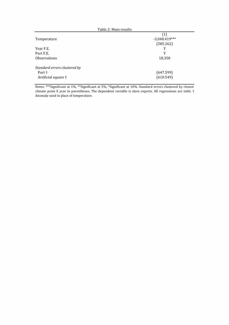
(1)Temperature -3,048.419***

(585.262)Year F.E. YPort F.E. YObservations 18,358

Standard errors clustered by Port † (647.599) Artificial square † (610.549)

Notes: ***Significant at 1%, **Significant at 5%, *Significant at 10%. Standard errors clustered by closest

climate point X year in parentheses. The dependent variable is slave exports. All regressions are tobit. †

Anomaly used in place of temperature.

Table 2: Main results

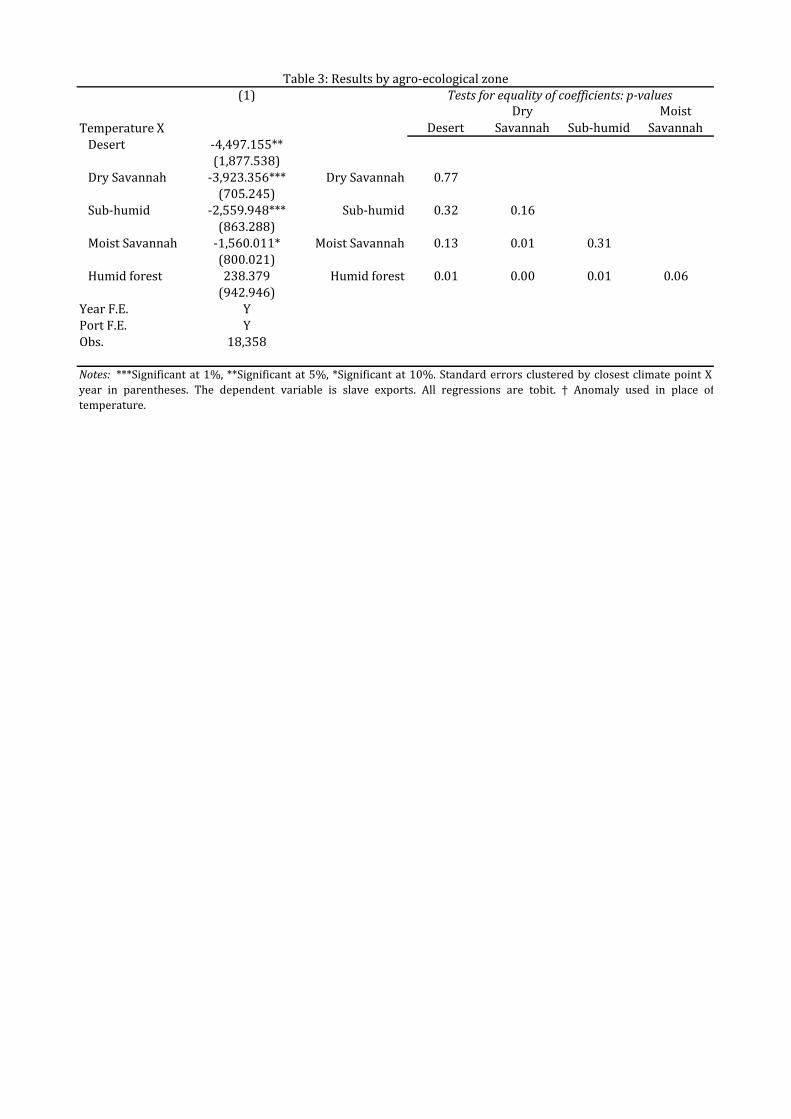
(1)

Temperature X Desert

Dry

Savannah Sub-humid

Moist

Savannah

Desert -4,497.155**(1,877.538)

Dry Savannah -3,923.356*** Dry Savannah 0.77(705.245)

Sub-humid -2,559.948*** Sub-humid 0.32 0.16(863.288)

Moist Savannah -1,560.011* Moist Savannah 0.13 0.01 0.31(800.021)

Humid forest 238.379 Humid forest 0.01 0.00 0.01 0.06(942.946)

Year F.E. YPort F.E. YObs. 18,358

Table 3: Results by agro-ecological zone

Notes: ***Significant at 1%, **Significant at 5%, *Significant at 10%. Standard errors clustered by closest climate point X

year in parentheses. The dependent variable is slave exports. All regressions are tobit. † Anomaly used in place of

temperature.

Tests for equality of coefficients: p-values

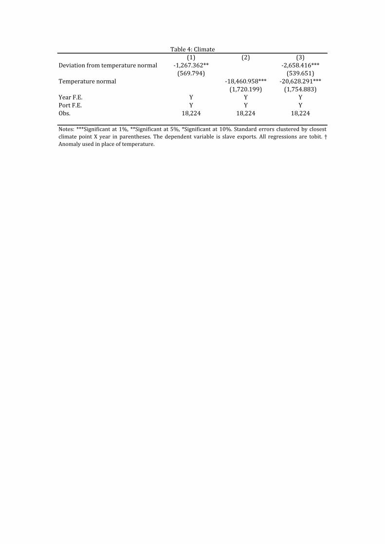
(1) (2) (3)Deviation from temperature normal -1,267.362** -2,658.416***

(569.794) (539.651)Temperature normal -18,460.958*** -20,628.291***

(1,720.199) (1,754.883)Year F.E. Y Y YPort F.E. Y Y YObs. 18,224 18,224 18,224

Table 4: Climate

Notes: ***Significant at 1%, **Significant at 5%, *Significant at 10%. Standard errors clustered by closest

climate point X year in parentheses. The dependent variable is slave exports. All regressions are tobit. †

Anomaly used in place of temperature.

Heterogeneity Measurement

Linear port trends -1,683.249*** Known slaves -1,848.411***(524.118) (427.755)

Obs. 18,358 Obs. 18,358

Quadratic region trends † -1,708.808*** Known slaves + Region known -2,131.973***(548.612) (440.114)

Obs. 18,358 Obs. 18,358

Pre-1807 -2,127.189*** Closest temperature point -2,636.976***(514.927) (508.351)

Obs. 10,318 Obs. 18,358

Post-1806 -2,191.992** Level of observation(938.323) Artificial squares (1x1) -3,178.098***

Obs. 8,040 (617.853) Obs. 16,166

Active ports only † -2,315.232***(595.612) Artificial squares (5x5) -5,519.570***

Obs. 6,780 (1,307.552) Obs. 3,973

Control for New World Temperature -3,086.413***(586.896) Region-level -11,203.841***

Obs. 18,358 (3,561.971) Obs. 1,096

Control for New World Prices -2,222.808***(488.278) Outliers

Obs. 10,854 No high dfbeta -1,979.578***(342.342)

Temperature shock at modal destination -3,290.472*** Obs. 17,826(546.155)

Obs. 17,536 Top 50% of ports -3,283.250***(618.649)

Obs. 9,179

Top 50% of years by port -1,893.247***(525.018)

Obs. 9,246

Table A1: Robustness checks 1

Notes: ***Significant at 1%, **Significant at 5%, *Significant at 10%. Standard errors clustered by closest climate point X year in parentheses.

The dependent variable is slave exports. All regressions are tobitwith port and year fixed effects unless otherwise indicated. † Anomaly used in

place of temperature.

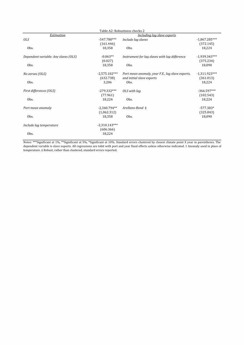
Estimation Including lag slave exports

OLS -547.780*** Include lag slaves -1,867.285***(161.446) (372.145)

Obs. 18,358 Obs. 18,224

Dependent variable: Any slaves (OLS) -0.063** Instrument for lag slaves with lag difference -1,939.343***(0.027) (375.234)

Obs. 18,358 Obs. 18,090

No zeroes (OLS) -2,575.102*** -1,311.923***(632.738) (361.013)

Obs. 3,206 Obs. 18,224

First differences (OLS) -279.332*** OLS with lag -366.597***(77.961) (102.543)

Obs. 18,224 Obs. 18,224

Port mean anomaly -2,340.794** Arellano-Bond ‡ -577.383*(1,062.312) (325.843)

Obs. 18,358 Obs. 18,090

Include lag temperature -2,310.143***(606.366)

Obs. 18,224

Table A2: Robustness checks 2

Notes: ***Significant at 1%, **Significant at 5%, *Significant at 10%. Standard errors clustered by closest climate point X year in parentheses. The

dependent variable is slave exports. All regressions are tobit with port and year fixed effects unless otherwise indicated. † Anomaly used in place of

temperature. ‡ Robust, rather than clustered, standard errors reported.

Port mean anomaly, year F.E., lag slave exports,

and initial slave exports

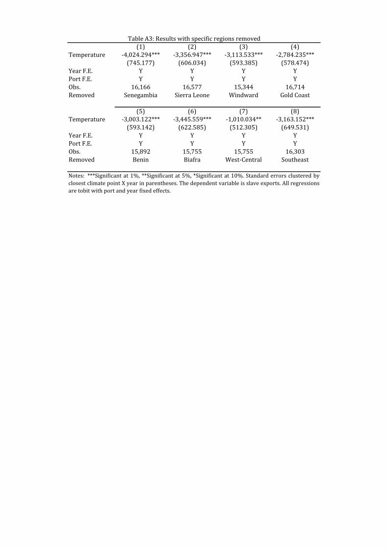
(1) (2) (3) (4)Temperature -4,024.294*** -3,356.947*** -3,113.533*** -2,784.235***

(745.177) (606.034) (593.385) (578.474)Year F.E. Y Y Y YPort F.E. Y Y Y YObs. 16,166 16,577 15,344 16,714Removed Senegambia Sierra Leone Windward Gold Coast

(5) (6) (7) (8)Temperature -3,003.122*** -3,445.559*** -1,010.034** -3,163.152***

(593.142) (622.585) (512.305) (649.531)Year F.E. Y Y Y YPort F.E. Y Y Y YObs. 15,892 15,755 15,755 16,303Removed Benin Biafra West-Central Southeast

Table A3: Results with specific regions removed

Notes: ***Significant at 1%, **Significant at 5%, *Significant at 10%. Standard errors clustered by

closest climate point X year in parentheses. The dependent variable is slave exports. All regressions

are tobit with port and year fixed effects.

Documents

Climate, ecosystem resilience and the slave trade