Embed Size (px)
Citation preview

CLIMATIC VARIATIONIN
EARTH HISTORY

CLIMATIC VARIATIONIN
EARTH HISTORY
Eric J. BarronEarth System Science Center
Pennsylvania State University
UNIVERSITY SCIENCE BOOKSSAUSALITO, CALIFORNIA

University Science Books
55D Gate Five Road
Sausalito, CA 94965
Fax: (415) 332-5393
Managing Editor: Lucy Warner
Editor: Louise Carroll
NCAR Graphics Team: Justin Kitsutaka, Lee Fortier, Wil Garcia,
Barbara Mericle, David McNutt, and Michael Shibao
Cover Design and Photography: Irene Imfeld
Compositor: Archetype Typography, Berkeley, California
This book is printed on acid-free paper.
Copyright © 1996 by University Corporation for Atmospheric
Research. All rights reserved.
Reproduction or translation of any part of this work beyond
that permitted by Section 107 or 108 of the 1976 United States
Copyright Act without the permission of the copyright owner is
unlawful. Requests for permission or further information should
be addressed to UCAR Communications, Box 3000, Boulder, CO
80307-3000.
Library of Congress Catalog Number: 95-061063
ISBN: 0-935702-82-2
Printed in the United States of America
10 9 8 7 6 5 4 3 2 1

A Note on the Global Change Instruction Program
This series has been designed by college professors to fill an
urgent need for interdisciplinary materials on the emerging
science of global change. These materials are aimed at
undergraduate students not majoring in science. The modular
materials can be integrated into a number of existing courses
—in earth sciences, biology, physics, astronomy, chemistry,
meteorology, and the social sciences. They are written to capture
the interest of the student who has little grounding in math
and the technical aspects of science but whose intellectual
curiosity is piqued by concern for the environment. The material
presented here should occupy about two weeks of classroom
time.
For a complete list of modules available in the Global Change
Instruction Program, contact University Science Books, Sausalito,
California, fax (415) 332-5393. Information about the Global
Change Instruction Program is also available on the World Wide
Web at http://home.ucar.edu/ucargen/education/gcmod/
contents.html.

ContentsPreface ix
Climatic Variation in Earth History 1
First Case Study. Plate Tectonics and Climate:
Episodes of Extensive Glaciation and Extreme Global Warmth 3
Plate Tectonics and the Surface Earth 3
How Can Plate Tectonics Influence Global Climate 6
Modeling to Explain the Extreme Warmth of the Cretaceous 9
Second Case Study. The Orbit of Earth and Pleistocene Glacial Rhythms 13
The Orbital Elements and the Insolation of Earth 15
Explanations of Glacial Rhythms 17
Summary 21
Glossary 22
Recommended Reading 23
Index 24

ix
Preface
The geologic record contains a rich and diverse history of
climatic change. This module presents two case studies from
Earth history and describes only a small sample of the recorded
inventory of trends and events that can contribute to our
understanding of Earth as a system—as a set of interacting
processes that operate over a wide range of space and time
scales. The first case study examines the contrasts between
major episodes of warm, apparently ice-free climates and times
of major glaciation. The second case study examines the
rhythms within the most recent period of glacial climate. The
primary driving forces and their time scales are very different in
the two case studies, but each provides substantial insight into
the sensitivity of Earth to change. In both cases, the primary
forcing factor pertinent to each process is insufficient to cause
the “signal” recorded in the geologic record, and, therefore, we
must understand a host of other factors.
Eric J. Barron, Director
Pennsylvania State University

Acknowledgments
This instructional module has been produced by the the Global
Change Instruction Program of the Advanced Study Program of
the National Center for Atmospheric Research, with support
from the National Science Foundation. Any opinions, findings,
conclusions, or recommendations expressed in this publication
are those of the author and do not necessarily reflect the views of
the National Science Foundation.
Executive Editors: John W. Firor, John W. Winchester
Global Change Working Group
Louise Carroll, University Corporation for Atmospheric Research
Arthur A. Few, Rice University
John W. Firor, National Center for Atmospheric Research
David W. Fulker, University Corporation for Atmospheric Research
Judith Jacobsen, University of Denver
Lee Kump, Pennsylvania State University
Edward Laws, University of Hawaii
Nancy H. Marcus, Florida State University
Barbara McDonald, National Center for Atmospheric Research
Sharon E. Nicholson, Florida State University
J. Kenneth Osmond, Florida State University
Jozef Pacyna, Norwegian Institute for Air Research
William C. Parker, Florida State University
Glenn E. Shaw, University of Alaska
John L. Streete, Rhodes College
Stanley C. Tyler, University of California, Irvine
Lucy Warner, University Corporation for Atmospheric Research
John W. Winchester, Florida State University
xi
This project was supported, in part, by the
National Science FoundationOpinions expressed are those of the authors
and not necessarily those of the Foundation

CLIMATIC VARIATIONIN
EARTH HISTORY
1
Climatic Variation in Earth History
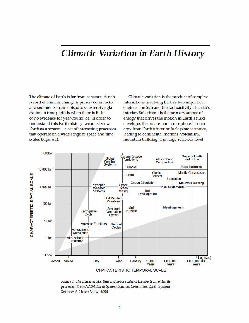
The climate of Earth is far from constant. A rich
record of climatic change is preserved in rocks
and sediments, from episodes of extensive gla-
ciation to time periods when there is little
or no evidence for year-round ice. In order to
understand this Earth history, we must view
Earth as a system—a set of interacting processes
that operate on a wide range of space and time
scales (Figure 1).
Climatic variation is the product of complex
interactions involving Earth’s two major heat
engines, the Sun and the radioactivity of Earth’s
interior. Solar input is the primary source of
energy that drives the motion in Earth’s fluid
envelope, the oceans and atmosphere. The en-
ergy from Earth’s interior fuels plate tectonics,
leading to continental motions, volcanism,
mountain building, and large-scale sea-level
Figure 1. The characteristic time and space scales of the spectrum of Earth
processes. From NASA Earth System Sciences Committee, Earth System
Science: A Closer View, 1988.
Volcanic Eruptions
Carbon-DioxideVariations
Climate
AtmosphericComposition
Origin of Earthand of Life
GlacialPeriodsEl Niño
Plate Tectonics
Mantle Convections
Speciation
Mountain BuildingOcean Circulation
SoilDevelopment
Extinction Events
Metallogenesis
Soil MoistureVariations
SoilErosion
SeasonalVegetationCycles
NutrientCycles
EarthquakeCycle
AtmosphericConvection
AtmosphericTurbulence
Global
10,000 km
1,000 km
100 km
10 km
1 km
Local
CHARACTERISTIC SPATIAL SCALE
CHARACTERISTIC TEMPORAL SCALE
Second Minute Day Year Century 10,000Years
1,000,000Years
1,000,000,000Years
Log (sec)
SynopticWeatherSystems
GlobalWeatherSystems
UpperOceanMixing
2
CLIMATIC VARIATION IN EARTH HISTORY
variations. The interactions between the solid
Earth and the fluid Earth are reflected in the
surface features of Earth and define the reser-
voirs and fluxes of biogeochemical cycles. The
climatic record appears best explained by a
combination of more than one of three basic
factors: (1) the amount and distribution of solar
energy received at the top of the atmosphere,
(2) the composition of the atmosphere, and
(3) the nature of the surface of Earth.
Two “case studies” of climate and climatic
change during Earth history illustrate this view
of the Earth system. One involves the major
episodes of glaciation and extreme warmth,
and the second examines the glacial rhythms
within the current episode of glaciation. Inter-
estingly, although the primary driving forces
and their time scales are quite different, atmo-
spheric carbon dioxide appears to play a role in
each of the case studies.
As the two examples will illustrate, contin-
ued study of Earth’s rich record of climatic
change and Earth system interactions promises
to provide many new insights into global evo-
lution and the sensitivity of Earth to
change.

3
FIRST CASE STUDY
Plate Tectonics and Climate—Episodes of Extensive Glaciationand Extreme Global Warmth
The most persuasive evidence for global cli-
matic change in Earth history is the record
of extensive glaciations separated by periods
for which there is little or no evidence of year-
round ice (Figure 2). From an Earth-history
perspective, the climate of today is distinctly
glacial. Much of the research that attempts to
explain the major changes in climate, illustrated
in Figure 2, focuses on periods of the greatest
contrast. The warm climate of the Cretaceous
period (approximately 100 million years ago)
exhibits the largest well-documented contrast
to the present glacial climate.
The evidence for global warmth comes from
every facet of the geologic record including
paleontology, geochemistry, and sedimentol-
ogy. More than 400 plant species are recorded
from latitudes above the Arctic Circle, and these
polar floras are indicative of seasonal condi-
tions with mean annual temperatures between
5 and 10°C. Fossils of large ectotherms (cold-
blooded organisms) are found at latitudes as
high as 60 degrees, whereas we know that mod-
ern relatives (alligators and crocodiles) become
inactive below 20°C and are restricted to much
lower latitudes. In the marine realm, no evi-
dence of cold-water faunas from Cretaceous
time has been discovered. Paleotemperature
data suggest that deep ocean temperatures
were between 15 and 17°C, compared to mod-
ern values of 1–2°C. Tropical surface tempera-
tures were evidently similar to modern values,
or a few degrees higher. A combination of
these data (Figure 3) suggests that the globally
averaged surface temperatures were 6–12°C
higher than at present, with polar temperatures
20–50°C higher.
Not only did the Cretaceous show substan-
tially greater warmth over millions of years, but
the transition from the warm climatic condi-
tions of the Cretaceous to the modern glacial
climate occurred slowly, over tens of millions
of years. This evidence argues for a causative
mechanism that operates over a long time.
Since the formulation of the plate tectonic
theory of crustal evolution, the changing distri-
bution of continents has become a frequently
cited explanation for the occurrence of glacial
and nonglacial climates. The following sections
explain how.
Plate Tectonics and the Surface Earth
Earth’s crust (lithosphere) consists of a series
of rigid plates that are in extremely slow but
constant motion. Plate tectonics is defined sim-
ply as the interactions between these plates.
Three types of interactions occur: (1) two plates
diverge, and new lithospheric crust is created
from hot molten rock that moves up from be-
low; (2) plates converge, forcing one beneath
the other in a process known as subduction;
and (3) two plates slide past each other without

4
CLIMATIC VARIATION IN EARTH HISTORY
Geologic Time Scale
Era Period EpochYears Beforethe Present
Holocene(Recent)
11,000Quaternary
Pleistocene(Glacial)
Cenozoic
Tertiary
Mesozoic
Paleozoic
Precambrian
Cretaceous
Triassic
Jurassic
Permian
Pennsylvanian(Upper Carboniferous)
Mississippian(Lower Carboniferous)C
arboniferous
Devonian
Silurian
Ordovician
Cambrian
Pliocene
Miocene
Oligocene
Eocene
Paleocene
1,600,000
570,000,000
5,300,000
23,700,000
36,600,000
57,800,000
66,400,000
144,000,000
208,000,000
245,000,000
286,000,000
320,000,000
360,000,000
408,000,000
438,000,000
505,000,000
Proterozoic
Archean
2,500,000,000
3,800,000,000
Figure 3. Mean annual surface temperatures in
Cretaceous times, compared with modern values (after
Barron, 1983). Some of the major constraints are based on
oxygen isotopes (in benthic and planktonic Foraminifera,
bottom-dwelling and floating microorganisms that secrete
a CaCO3 shell, and belemnites, ancient relatives of a
nautilus), reef distribution, and the absence of year-
round ice.
N
4600
A
3000 2500 2000 1500 1000 900 800 700 600 500 400 300 200 100 0
Glacial Record of the Earth
EP LP C O S D C P T J K P
M.Y.B.P.Probable Age RangePossible Age Range
Figure 2, above and right. The probable time range
of glacial episodes during Earth history. Times of
uncertainty in interpreting the record are given as
possible ranges of glaciation.
80N 40 0 40 80S
0
40
30
20
10
-10
-20
-30
-40
-50
LATITUDE
TEMPERATURE (°C)
"Warmest" Cretaceous"Coolest" CretaceousPresent Day
No year-round ice
Belemnites
Reefs
PlanktonicForaminifera
BenthicForaminifera

5
convergence or divergence. The idealized
plate in Figure 4 includes both continental and
oceanic crust. The plate is growing with the
addition of new material (accretion) at the
midoceanic ridge on the right, and oceanic
crust is being destroyed (subducted) where
the idealized plate converges with the adjacent
plate on the far left. Throughout the world,
subduction is indicated by the distribution of
deep-sea trenches, by explosive volcanism, and
by deep-seated earthquakes. In Figure 4, the
ocean basin to the right of the continent is
growing in area while the ocean basin to the
left of the continent decreases in size.
One consequence of plate tectonics is that the
distribution of continents is continually chang-
ing. The Atlantic Ocean first formed about 165
million years ago, at which time the world con-
sisted of a single megacontinent, Pangaea, and
a single super-ocean called Panthalassa. We
can find times in Earth history when Greenland
straddled the equator and times when the
Sahara Desert was at the South Pole.
The topography or elevation of the conti-
nents is also governed by plate tectonics.
With continued motion of the plates, collision
between continents is inevitable. Usually, the
thinner and more dense oceanic lithosphere is
subducted beneath the thicker and less dense
continental lithosphere. For example, the exist-
ence of the Andes mountain range is a direct
consequence of South America’s being at the
boundary of an active or converging plate. The
Himalayan-Tibetan Plateau region, the highest
topography in the world, is the product of the
collision of India and Asia nearly 50 million
years ago.
Plate tectonics also influences sea level.
At boundaries where new crust is created (pre-
dominately at midocean ridges), hot, thick
lithosphere is accreted to the margins of diverg-
ing plates. Over tens of millions of years the
thick lithosphere cools and contracts. In fact, the
new crust is clearly evident as ridges (midocean
ridges) on maps of the depth of the ocean. Con-
sequently, at times when new sea floor is cre-
ated more rapidly by faster spreading at
divergent boundaries or increased length of
midocean ridges, the holding capacity of the
ocean basins decreases and some continental
flooding occurs. For example, most estimates
suggest that during the middle Cretaceous new
sea floor was created at a rate twice as fast as it
is today. The theory of lithospheric cooling and
contraction suggests that such a fast sea-floor
spreading rate would yield a global sea-level
rise of 200 to 300 meters (this may be compared
with 65 meters if we melted the modern ice
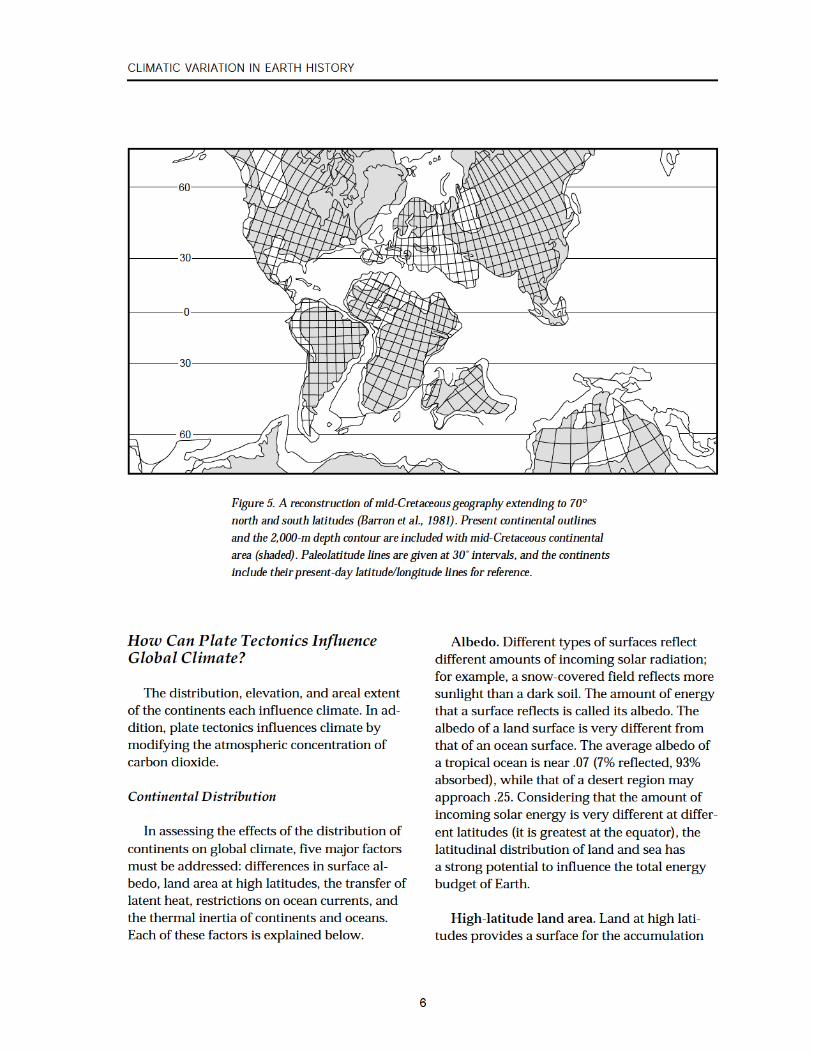
caps). In fact, almost 20% of the modern con-
tinents was covered by ocean in the middle
Cretaceous (Figure 5). In short, plate tectonic
processes affect not only the distribution and
elevation of the continents, but also the area
of continents above sea level.
Figure 4. From right to left, the motion of lithospheric plates in response to mantle convection.
Subduction:cooled lithosphere sinks
Lithosphere cools as it spreads
Mid-oceanicridge
Lithosphere formsfrom rising hot magma
Lithosphere remelts
TrenchOcea
n OceanContinental raft
Lithosphere
Asthenosphere(upper mantle)
70 km
PLATE TECTONICS AND CLIMATE
6
CLIMATIC VARIATION IN EARTH HISTORY
60
30
0
30
60
How Can Plate Tectonics InfluenceGlobal Climate?
The distribution, elevation, and areal extent
of the continents each influence climate. In ad-
dition, plate tectonics influences climate by
modifying the atmospheric concentration of
carbon dioxide.
Continental Distribution
In assessing the effects of the distribution of
continents on global climate, five major factors
must be addressed: differences in surface al-
bedo, land area at high latitudes, the transfer of
latent heat, restrictions on ocean currents, and
the thermal inertia of continents and oceans.
Each of these factors is explained below.
Albedo. Different types of surfaces reflect
different amounts of incoming solar radiation;
for example, a snow-covered field reflects more
sunlight than a dark soil. The amount of energy
that a surface reflects is called its albedo. The
albedo of a land surface is very different from
that of an ocean surface. The average albedo of
a tropical ocean is near .07 (7% reflected, 93%
absorbed), while that of a desert region may
approach .25. Considering that the amount of
incoming solar energy is very different at differ-
ent latitudes (it is greatest at the equator), the
latitudinal distribution of land and sea has
a strong potential to influence the total energy
budget of Earth.
High-latitude land area. Land at high lati-
tudes provides a surface for the accumulation
Figure 5. A reconstruction of mid-Cretaceous geography extending to 70°
north and south latitudes (Barron et al., 1981). Present continental outlines
and the 2,000-m depth contour are included with mid-Cretaceous continental
area (shaded). Paleolatitude lines are given at 30̊ intervals, and the continents
include their present-day latitude/longitude lines for reference.

7
of snow and year-round ice. Snow and ice have
a very high albedo; for fresh snow it approaches
.65 to .80. Consequently, high-latitude land
area, if snow-covered, can also dramatically
influence the energy budget of the atmosphere-
ocean system.
Transfer of latent heat. Changes in albedo
are not the only mechanism by which continen-
tal distribution affects the global energy budget
and, hence, the global climate. An examination
of the surface energy budget, in terms of sen-
sible and latent heat fluxes (Figure 6), reveals a
third means by which continental distribution
influences climate. The largest energy fluxes at
the surface of Earth involve moisture (latent
heat flux). Clearly, the distribution of land and
sea will influence evaporation and precipitation
and therefore the total energy budget of the
atmosphere.
Restrictions on ocean currents. Continents
act as barriers to the flow of oceanic currents.
The oceans transport a substantial amount of
heat poleward (a maximum of 2–4 x 10¹⁵ watts
at latitudes of 20–30 degrees, representing one-
third to one-half of the total poleward heat
transport by the oceans and the atmosphere).
The distribution of land can block poleward
heat transport by the ocean and may influence
polar climates and the subsequent extent of ice
and snow cover. Thus, the shape and size of the
ocean basins become a factor in controlling
global climate.
Thermal inertia. A continental surface has
little thermal inertia. Basically, a continental
surface responds rapidly to the current solar
input. In contrast, the oceans have a large heat
capacity. They store solar energy in summer
and release it in winter. Therefore, the thermal
inertia of the oceans tends to moderate the role
of the seasonal cycle of insolation. The range of
summer or winter temperatures could influence
whether or not snow accumulated in the winter
or melted in the summer. Again, in this ex-
ample, the distribution of land and sea may be
a controlling factor in the occurrence of glacial
or nonglacial climates.
R = Net Solar and IR Radiation (W/m2)E = Evaporation/Transpiration (W/m2)S = Sensible Heat (W/m2)α ≡ Surface Albedo
Subtropical Landα ≡0.25
50 15
Subtropical Oceanα ≡0.07
85 80 5
Near-Equatorial Landα ≡0.12
60 45 15
35
PLATE TECTONICS AND CLIMATE
R E S
Figure 6. Heat balances for some representative surface
types. On average, net radiative heating of the surface
is balanced by evaporative and sensible heat loss.
Evaporation is the preferred mode of heat loss at warm
temperatures; thus subtropical oceans lose heat mainly
through evaporation.
8
CLIMATIC VARIATION IN EARTH HISTORY
Continental Elevation
Climate is also influenced in a number of
ways by the elevation of continents. Examples
of this factor include temperature change and
varying moisture content with changing eleva-
tion, the effect of mountains on large-scale at-
mospheric circulation, the effect of mountains
on regional climate, and influences of topo-
graphy on the general circulation of the
atmosphere.
Effects of changing elevation. Atmospheric
temperature decreases with height, a decrease
referred to as the lapse rate. The average lapse
rate is 6.5°C per kilometer of height. The colder
temperatures at higher elevations promote
snow accumulation, and therefore mountains
become a base region for glaciation. Again,
snow and ice have a very high albedo, so the
occurrence of year-round snow and ice pro-
motes cooling through modification of the en-
ergy balance.
Effects on large-scale circulation. The distri-
bution of mountains influences the large-scale
circulation of the atmosphere. In the simplest
form, this influence is analogous to that of a
large rock in a stream. The rock acts as a barrier
to the flow of the fluid, and the current pattern
is modified around and downstream from the
barrier. The positions of the continents and
oceans (causing differences in heating) and the
distribution of regions of high topography con-
trol the position of the large-scale waves in the
atmosphere, such as the jet stream, and there-
fore control the pattern of the weather. A
change in topography may well control the
distribution of cold air masses or the track
of winter storms. Such changes could initiate
glaciation in a particular region by promoting
even greater cooling, or they could warm high-
latitude regions which may otherwise be cool.
Effects on regional climate. The regional
differences in climate associated with
topography might be considered a third mecha-
nism of climatic change. The windward sides of
mountains tend to be much wetter, while a
rain-shadow effect occurs in the lee of moun-
tains. On the windward side the air is forced
upward, cooling with increasing elevation.
Since cooler air can hold less moisture, the cool-
ing air mass reaches saturation and precipita-
tion occurs. In the lee, deserts develop because
the sinking air warms and therefore the level of
saturation decreases as the air descends. For
this reason, the different sides of mountain belts
tend to have very different climates.
Effects on general circulation. Topography
can exert an influence on the general circulation
of the atmosphere or large-scale wind patterns.
The general circulation is very complex, but it
can be understood by a series of thought experi-
ments. First, imagine a nonrotating Earth. On
average, the air near the equator is heated the
most and the air near the poles the least. In
response to this, the cold, dense air at the poles
sinks and spreads toward the equator, while
the air over the equator rises and moves toward
the poles. In this case the Northern Hemisphere
winds near the surface would be from the north
and the winds at higher altitudes would be
from the south.
What happens if Earth rotates about its axis?
Every point on Earth makes a complete circuit
in a day. Near the poles, each point on the
Earth’s surface hardly moves; points on the
equator, being farthest from Earth’s axis, move
most rapidly. What does this mean for the
wind? Consider the case of air moving north-
ward from the equator. The surface north of the
equator moves more slowly, so the air moves
toward the east—the winds are now from the
southwest instead of the south. Similarly, the
sinking cold air at the poles has almost no east-
ward speed, but south of the pole, the surface
beneath moves eastward faster. Thus the polar
air, which started out moving southward, be-
gins to turn southwestward. The winds are
from a northeasterly direction.
9
Because of the rotation of Earth, the circula-
tion in each hemisphere tends to be broken up
into three cells. On the surface of the Northern
Hemisphere, the winds near the poles are from
the northeast (the polar easterlies), and the
winds near the equator are from the northeast
(the northeast trade winds). They are separated
by a broad zone of west winds in the middle
latitudes (the midlatitude westerlies). The east-
erlies and westerlies exert a frictional drag on
the surface of the earth that must balance.
Now let’s add mountain belts. A mountain
belt in the easterly wind belt would exert a
westward frictional drag on the winds. The
opposite would occur in the region of the west-
erlies. Differences in pressure across mountains
would play a role similar to the frictional drag.
Therefore, the strength and the distribution of
the easterlies and westerlies would change for
an Earth with fewer mountains or a different
distribution of mountains.
Carbon Dioxide and Plate Tectonics
There are numerous mechanisms by which
aspects of plate tectonics directly modify the
atmospheric or oceanic circulation, or directly
influence the surface energy balance (albedo
changes). Plate tectonic processes also modify
the carbonate-silicate geochemical cycle.
Increased sea-floor spreading rates and in-
creased plate destruction by subduction (faster
plate tectonic processes) should result in greater
outgassing of carbon dioxide from volcanoes.
On long time scales, carbon dioxide production
is balanced by consumption during weathering
of igneous and metamorphic rocks. To maintain
the atmospheric carbon dioxide concentration,
the amount of carbon dioxide consumed by
silicate weathering would also have to increase.
Many researchers suggest that during the Cre-
taceous the rate of sea-floor spreading was
nearly twice as great as the modern rate.
In addition, as stated earlier, higher rates of
plate accretion are associated with higher sea
level. For those times for which much higher
sea-floor spreading rates are hypothesized, in-
creased continental flooding should occur (e.g.,
covering 20% of the present-day continental
area in the middle Cretaceous). Consequently,
not only was it likely that volcanic outgassing
of carbon dioxide was higher than today, but
the area of continental rocks exposed that
would consume atmospheric carbon dioxide
through the weathering of silicate rocks was
substantially less.
This simple argument suggests that changes
in the rates of plate tectonic processes can pro-
duce changes in the atmospheric concentration
of the important greenhouse gas carbon diox-
ide. Such changes would occur on a time scale
of tens of millions of years. Interestingly, the
times of high sea level are often associated with
planetary warmth and the times of low sea level
are associated with cooler climates. This asso-
ciation may reflect the fact that atmospheric
carbon dioxide concentration is tied to plate
tectonics as part of the carbonate-silicate cycle.
Modeling to Explain the ExtremeWarmth of the Cretaceous
A large number of mechanisms related to
plate tectonics may be responsible for, or con-
tribute to, the occurrence of major glaciations or
extreme climatic warmth in Earth history. Cli-
mate models provide an opportunity to probe
whether any specific forcing factor has been
important in regulating past climates. Models
are mathematical representations of the climate
system. By changing a specific factor, such as
land-sea distribution, a scientist can examine
the model response and compare it with the
information derived from the geologic record.
Evaluation of all the mechanisms described
above is not straightforward. In fact, multiple
mechanisms may be responsible for changes
in climate, and there is no reason to suppose
that the same mechanism produced each of the
major climatic episodes illustrated in Figure 2.
Since the changes in Cretaceous geography are
PLATE TECTONICS AND CLIMATE

10
CLIMATIC VARIATION IN EARTH HISTORY
Figure 7. A comparison of the zonally averaged surface
temperature (averaged across latitudinal belts) for the
present-day control and “realistic” Cretaceous simulation.
large and well known (Figure 5), study of the
effects of the distribution of land and sea is a
logical starting point to try to explain Creta-
ceous warmth. In order to assess the impor-
tance of geography, the model results can be
compared with the surface temperature data
plotted in Figure 3.
Paleogeography and Cretaceous Warmth
A hierarchy of climate models, from simple
two-dimensional models that consider only
the equator-to-pole temperature contrast to
three-dimensional models that simulate the
atmospheric circulation, has been applied to
the study of the extreme climatic warmth of the
Cretaceous. The results from each type of
model simulation suggest that Cretaceous land-
sea distribution is an important factor contrib-
uting to the extreme warmth. For example, one
of the most comprehensive models of the atmo-
sphere has been utilized to simulate the climate
for the Cretaceous, based on the geography
illustrated in Figure 5. The global average tem-
perature for a simulated Cretaceous climate,
based on this geography and without polar ice
caps, was 4.8°C higher than for a present-day
control simulation. The warming was accentu-
ated at high latitudes (Figure 7 shows a 15°C
and 35°C increase at high northern and south-
ern latitudes, respectively), corresponding very
closely to the sense of the warming estimated
from the geologic record. However, this result
is problematic. Even though the warming is in
the right sense, the magnitude is only half of
what is required to explain the geologic
evidence.
Interpreting the result is more difficult
because the simulated Cretaceous warming
includes changes in several different model
parameters at once (continental positions, to-
pography, sea level, and removal of the ice
caps), relative to the present-day control simu-
lation. What factors are responsible for the
4.8°C warming? Modelers attempt to dissect
such complex cause-and-effect relationships by
repeating the experiments, changing only one
variable at a time to determine which were
most responsible for the net change.
Interestingly, as Figure 8 shows, the warm-
ing of the Southern Hemisphere was due al-
most entirely to the removal of the Antarctic
ice cap. (Remember that the difference between
warm, ice-free climates and glacial climates is
what we are trying to explain, yet the total
simulated temperature difference at high south-
ern latitudes seems to be associated with the
removal of ice rather than some geographic
factor!) Most of the Northern Hemisphere
warming can be attributed to the difference in
the amount of high-latitude land. The model
showed no sensitivity to sea level, and although
topography played an important role in gov-
erning regional climates, removal of all mod-
ern-day topography did not result in a
substantial change in the global temperature.
The results of the climate model experiments
are of considerable interest, and there are sev-
eral possible ways to interpret them. First, as-
sume that the model simulations are accurate.
Clearly, then, the actual geographic changes
result in only a modest Northern Hemisphere
60N 30 0 30 60S
0
40
20
-20
-40
LATITUDE
TEMPERATURE (°C)
Present Day ControlCretaceous

11
Figure 8. (a) A comparison of the zonally averaged surface
temperature for the present-day simulation with and
without specified permanent snow (fixed high albedo) on
Antarctica and Greenland. (b) A comparison of the zonally
averaged surface temperature for the present-day
simulation with mountains and without mountains.
Mountains
No mountains
Specified snow
No specified snow
40 0 40 80S
0
30
20
-20
LATITUDE
TEMPERATURE (°C)
10
80N
0
40
20
-40
TEMPERATURE (°C)
-20
(a)
(b)
warming and the cause of the difference be-
tween global warmth and glaciation remains
unsolved. Some additional mechanism would
be required to explain the extreme warmth of
the Cretaceous. Alternatively, assume that the
geologic data is in substantial error. Certainly
many difficulties are associated with determin-
ing the temperatures prior to the historical
record. However, the model-simulated
warming deviates considerably from the ob-
servations; the simulations are well below even
the lower limit of the geologic interpretations.
Second, assume that the modern climate
models that are used here to simulate the Cre-
taceous climate may be missing some funda-
mental process or feedback mechanism, and
therefore are unable to correctly simulate cli-
mates very different from today’s. This is a very
real possibility as mathematical models are
highly idealized representations of the climate.
For example, the role of the oceans and the
characteristics of the ice caps are poorly repre-
sented in many climate models. Some research-
ers have suggested that the role of the oceans,
with their tremendous ability to store heat, is a
key to the problem. Because of this storage of
heat, oceanic regions have a smaller seasonal
change in temperature than land areas at the
same latitude. Using an energy balance climate
model, Thomas Crowley and his colleagues
demonstrated that the presence of oceanic re-
gions near the poles can reduce summer tem-
peratures over adjacent polar continental
regions in comparison with situations of high
polar continentality (see their article in Recom-
mended Additional Reading). These research-
ers suggested that cooler summer temperatures
may not melt winter snow and ice, thus initiat-
ing glaciation. The results suggest that the role
of geography has not yet been fully explored
and that the models must link the oceans, the
atmosphere, and the ice caps in order to pro-
vide an understanding of the history of Earth’s
climate.
What is the solution? Is the geologic record
misinterpreted? Are models far too inaccurate?
Do we need some additional forcing factor? The
geological record and the model simulations
provide one additional clue that helps to focus
the investigation. Remember that global
warmth appears to be well correlated with
times of high sea level, yet the climate model
results described earlier exhibited almost no
response in an experiment that flooded 20%
PLATE TECTONICS AND CLIMATE

12
CLIMATIC VARIATION IN EARTH HISTORY
and that higher levels in the Cretaceous are
likely, there are no accurate measurements of
atmospheric gas concentrations for periods tens
of millions of years ago. However, continued
experimentation with the climate model sug-
gests that quadrupling the atmospheric carbon
dioxide level in the Cretaceous, in addition to
the differences in geography, could produce an
8°C increase in temperature compared to the
present. For the first time the model-simulated
temperatures (Figure 9) are close to the limits
of the observations from the geologic record. A
quadrupled level of carbon dioxide for the Cre-
taceous is well within the limits suggested by
the geochemical models of the carbonate-
silicate cycle.
Of course, improved models may give very
different results. The carbon dioxide level re-
quired to achieve the extreme climatic warmth
of the Cretaceous may be greater than or less
than four times the present level. More impor-
tantly, the experiments suggest that several
factors are required to explain the climate of
a single time period, and, significantly, the
mechanisms are interrelated. Earth’s internal
heat engine, which drives plate tectonics, alters
climate directly through interactions of the at-
mosphere and oceans with the surface of Earth,
and indirectly through geochemical interactions
that alter the greenhouse character of the
atmosphere. Both the direct effects of plate
tectonics and the influence of plate tectonics on
geochemical processes are required, in concert,
to explain the large-scale changes in climate—
from episodes of extreme warmth to the major
periods of polar glaciation.
of the area of the continents. This point suggests
that something fundamental is missing from
our simulation. We then remember that times
of continental flooding are associated with
rapid sea-floor spreading rates, and presumably
higher carbon dioxide degassing rates.
Carbon Dioxide and Cretaceous Warmth
Although the geochemical models of the
carbonate-silicate cycle indicate that changes in
atmospheric carbon dioxide levels are plausible
Figure 9. A comparison of the estimates of Cretaceous
temperature limits (dotted lines) with predicted zonally
averaged surface temperatures for Cretaceous geography
(solid line) and for Cretaceous geography plus quadrupled
carbon dioxide (dashed line). Predicted temperatures were
derived from a general circulation model of the atmosphere
(Barron and Washington, 1984).
Estimated Cretaceous temperature limits
Cretaceous geography
Cretaceous geography and 4 x CO2
60N 30 0 30 60S
0
40
30
20
-10
LATITUDE
TEMPERATURE (°C)
50
10

13
SECOND CASE STUDY
The Orbit of Earth andPleistocene Glacial Rhythms
The first unequivocal evidence of a large
Antarctic ice cap is the occurrence of ice-rafted
detritus in deep-sea cores dated at 28 million
years of age. (Ice-rafted detritus is an indicator
that continental ice carrying material eroded
from the continents was transported out to sea
by icebergs.) Greenland was clearly glaciated
3 million years ago. A closer examination of the
record of glaciation during the last 1.9 million
years (the Pleistocene) reveals considerable
climatic variability in the form of repeated ad-
vances and retreats of the polar ice caps.
The movement of ice over the land surface is
an extremely destructive process, mechanically
grinding the rock surface and carrying the gla-
cial debris downstream. On land the history of
glaciation is recorded by glacial tracks and
scours and by the deposition of glacial debris
at the front (terminal moraines) and sides of
glaciers and ice caps. In North America and
Europe four major groups of terminal or end
moraines are preserved from the Pleistocene.
Does this record suggest four major glacial ad-
vances of the modern ice cap? Moraines
give scientists only the evidence of the farthest
extent of glaciation. A more recent glaciation
would destroy the record of any previous ice
age where the maximum extent of the ice was
less than that of the most recent advance. Until
1950, the end moraines were the only record of
the ice age, and only four major glaciations
were identified.
A much better record was derived from the
deep sea with the invention of coring devices in
1950. The coring of oceanic sediments retrieved
a continuous record of microscopic fossil shells
composed of calcium carbonate (CaCO3). This
new-found record was examined in detail with
an innovative chemical methodology based on
isotopes.
A chemical element is defined by the number
of protons in its nucleus. The number of neu-
trons in the nucleus can vary. Isotopes are ele-
ments with different mass numbers defined by
the total number of neutrons and protons. Be-
cause isotopes have different masses, different
physical and chemical processes may separate,
or fractionate, them. For example, oxygen has
three isotopes: oxygen-16, -17, and -18. In the
process of evaporation from the surface of the
ocean, water containing oxygen with the light-
est isotope value is preferentially evaporated.
Likewise, in precipitation there is a preference
to rain out water with the heaviest isotope,
oxygen-18, first. The atmosphere is, in a sense,
distilling the oxygen isotopic composition of the
moisture it transports through the processes of
evaporation and precipitation. The moisture
that is finally deposited on the ice caps is ex-
tremely enriched in the light isotope, and there-
fore, during times of extensive glaciation, the
ocean becomes depleted in oxygen-16. The mi-
croscopic organisms in the ocean that grow
CaCO3 shells preserve the oxygen isotopic com-
position of the oceanic water in which they live
and build their shells.
The record of oxygen isotopes for the last
700,000 years (Figure 10) reveals a remarkably

14
CLIMATIC VARIATION IN EARTH HISTORY
rhythmic record of repeated glaciation. More
oxygen-18 recorded by shells indicates more of
the lighter oxygen-16 stored as ice on land. Note
that the oxygen-18 record for each ice age has a
similar amplitude and that the record for each
ice age has a ramp-like structure suggesting
slow buildup to full glaciation and then rapid
retreat. The current climate is best described as
“interglacial” and the last major ice advance
(“glacial”) was approximately 18,000 years ago.
A wide variety of theories has been pre-
sented to explain these glacial cycles, involving
Earth orbital variability, volcanism, variations
in the magnetic field of Earth, solar variability,
interstellar dust, internal oscillations, Antarctic
ice surges, atmospheric carbon dioxide concen-
tration, and deep ocean circulation changes.
The remarkably rhythmic nature of the glacial
cycles, undiscovered until more complete
records from the deep sea were collected,
has proven to be a major test for the theories
of glaciation. A deterministic view of the cli-
matic system would suggest that the glacial-
interglacial rhythms were the product of some
periodic climatic forcing factor.
In the first half of the twentieth century,
Milutin Milankovitch, a Yugoslavian astrono-
mer, proposed that periodic changes in Earth’s
orbital characteristics were the major control
over glaciation. Milankovitch computed
periods for the variation in the time of year
during which Earth is closest to the Sun,
governed by the orbital precession of the equi-
noxes (approximately 19,000 to 23,000 years—
see discussion below); the axial tilt of Earth
approximately 41,000 years); and the eccentric-
ity of Earth’s orbit around the Sun (approxi-
mately 100,000 years). Milankovitch’s
hypothesis was rejected at the time due to the
weight of evidence from continental regions
suggesting that there were only four major
glaciations.
James Hays, John Imbrie, and Nick
Shackleton revitalized the Milankovitch hy-
pothesis when they calculated the timing of
variations for three geologic factors—surface
temperature, oxygen isotopes, and the abun-
dance of a particular plankton species—from
high-resolution, continuous deep-sea cores
representing the last 700,000 years (see their
paper in the Recommended Additional Read-
ing). They found that these variables illustrated
a rhythm with intervals of 19,000, 24,000,
43,000, and 100,000 years (Figure 11). The domi-
nant climatic periodicity is 100,000 years. The
correspondence of the periods from the geo-
logic data with the periods of the Earth’s orbital
characteristics is unmistakable.
Figure 10. Oxygen isotopic record for the last 700,000 years, illustrating
glacial/interglacial cycles (after Emiliani, 1978). Higher oxygen-18 levels show
interglacial periods.
Change in Oxygen-18 Isotopes
(parts per thousand)
1
0
0 100 200 300 400 500 600 700
Age ∞ 1,000 Years

15
The Orbital Elements andthe Insolation of Earth
The gravitational effects of the planets within
our solar system perturb the orbit of Earth.
Since the input of solar energy is dependent on
the distance between Earth and Sun and on
the solar angle, these orbital changes alter the
seasonal and latitudinal distribution of incom-
ing solar energy (called insolation).
Eccentricity
Due largely to interactions with Jupiter and
Saturn, the orbit of Earth about the Sun varies
from a circle (an eccentricity of 0) to an ellipse
(a maximum eccentricity of .07), with a period
of 96,600 years (Figure 11a). The Sun is cur-
rently nearest Earth in January and farthest
away in July. During periods of maximum ec-
centricity, the differences in Earth-Sun distance
from summer to winter can greatly accentuate
the contrast between the seasons. However,
on an annual average, variations in the eccen-
tricity result in less than a 1% range in the total
insolation.
Figure 11a. The orbit of Earth changes shape from nearly
circular to more elliptical. This is termed eccentricity and
is expressed as a percentage (after Imbrie and Imbrie,
1979).
Ellipses with different eccentricities
Changing shape of the ellipse
Earth Sun
040%
55%
65%
75%
Figure 11b. Variation in the tilt of Earth’s axis from
maximum to minimum, and the effect of axial tilt on the
distribution of sunlight. When the tilt is decreased from its
present value of 23.5°, the polar regions, in summer,
receive less sunlight; when the tilt is increased, polar
regions receive more sunlight (after Imbrie and Imbrie,
1979).
N
S
N
S
N
S
N
S
N
S
SUN
SUN
SUN
N
S
Tilt = 0°
Tilt = 54°
Tilt = 23.5°
EquatorialPlaneof Earth
June 21 December 21
OrbitPlane of
Present
Minimum Tilt
Maximum Tilt
THE ORBIT OF EARTH AND PLEISTOCENE GLACIAL RHYTHMS

16
CLIMATIC VARIATION IN EARTH HISTORY
Figure 11c: Precession of the equinoxes. Owing to axial
precession and to other astronomical movements, the
positions of equinox (March 20 and September 22) and
solstice (June 21 and December 21) shift slowly around
Earth’s elliptical orbit, and complete one full cycle about
every 22,000 years. Eleven thousand years ago, the winter
solstice occurred near one end of the orbit. Today, the
winter solstice occurs near the opposite end of the orbit.
Figure 12. Variations in Earth’s orbital elements,
eccentricity, tilt (obliquity), and time of perihelion
(precession of the equinoxes) computed for the last 500,000
years with a computer program written by Tamara Ledley
and Starley Thompson following Berger (1988).
Obliquity
The obliquity of Earth is measured as the tilt
of Earth’s axis from the normal to the plane of
its orbit (Figure 11b). Today the obliquity is 23.4
degrees (the latitude of the tropics of Cancer
and Capricorn). With a period of 41,000 years
the obliquity varies from 22 degrees to 24.5
degrees. The condition of higher obliquity
(greater tilt toward and away from the Sun)
produces more pronounced differences be-
tween winter and summer seasons and greater
total solar energy at the polar region. The con-
dition of low obliquity (less tilt) reduces the
seasonal cycle, but a smaller amount of insola-
tion is received in polar regions during the year.
The variation in obliquity produces a difference
of approximately 10% in polar insolation.
Precession of the Equinoxes
Solar and lunar torques on the equatorial
bulge of Earth cause the time of perihelion (the
time at which Earth is closest to the Sun) to vary
MAR. 20MAR. 20
DEC. 21
SEPT. 22
TODAY
JUNE 21
DEC. 21
SEPT. 22
JUNE 21
5,500 YEARS AGO
MAR. 20
SEPT. 22
JUNE 21
MAR. 20
11,000 YEARS AGO
DEC 21
ECCENTRICITY
TIME OF PERIHELIONTILT (deg)
TIME BEFORE PRESENT (1,000 yrs)
SEP
DEC
MAR
JUN
SEP
23
22
24
25
0
0.02
0.04
0.06
500 400 300 200 100 0
ORBITAL ELEMENTS
17
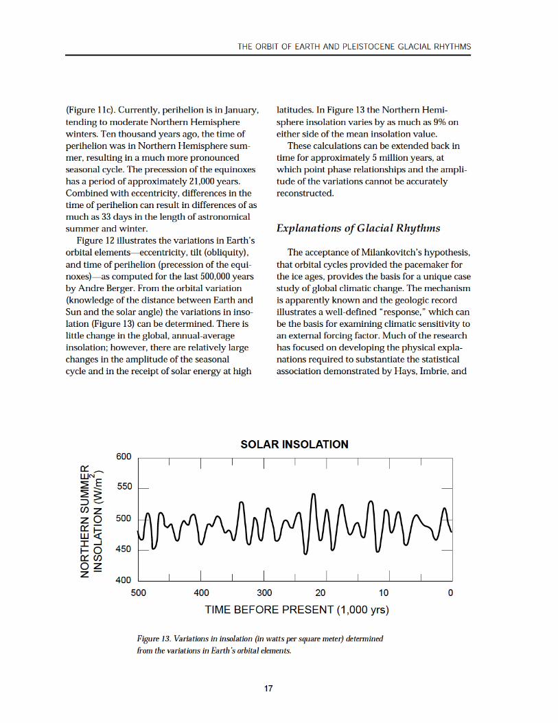
Figure 13. Variations in insolation (in watts per square meter) determined
from the variations in Earth’s orbital elements.
(Figure 11c). Currently, perihelion is in January,
tending to moderate Northern Hemisphere
winters. Ten thousand years ago, the time of
perihelion was in Northern Hemisphere sum-
mer, resulting in a much more pronounced
seasonal cycle. The precession of the equinoxes
has a period of approximately 21,000 years.
Combined with eccentricity, differences in the
time of perihelion can result in differences of as
much as 33 days in the length of astronomical
summer and winter.
Figure 12 illustrates the variations in Earth’s
orbital elements—eccentricity, tilt (obliquity),
and time of perihelion (precession of the equi-
noxes)—as computed for the last 500,000 years
by Andre Berger. From the orbital variation
(knowledge of the distance between Earth and
Sun and the solar angle) the variations in inso-
lation (Figure 13) can be determined. There is
little change in the global, annual-average
insolation; however, there are relatively large
changes in the amplitude of the seasonal
cycle and in the receipt of solar energy at high
latitudes. In Figure 13 the Northern Hemi-
sphere insolation varies by as much as 9% on
either side of the mean insolation value.
These calculations can be extended back in
time for approximately 5 million years, at
which point phase relationships and the ampli-
tude of the variations cannot be accurately
reconstructed.
Explanations of Glacial Rhythms
The acceptance of Milankovitch’s hypothesis,
that orbital cycles provided the pacemaker for
the ice ages, provides the basis for a unique case
study of global climatic change. The mechanism
is apparently known and the geologic record
illustrates a well-defined “response,” which can
be the basis for examining climatic sensitivity to
an external forcing factor. Much of the research
has focused on developing the physical expla-
nations required to substantiate the statistical
association demonstrated by Hays, Imbrie, and
NORTHERN SUMMER
INSOLATION (W/m2)
400
500 400 300 20 010
450
500
550
600
TIME BEFORE PRESENT (1,000 yrs)
SOLAR INSOLATION
THE ORBIT OF EARTH AND PLEISTOCENE GLACIAL RHYTHMS

18
CLIMATIC VARIATION IN EARTH HISTORY
Shackleton in 1976 (see their paper in the Rec-
ommended Additional Reading).
The complex general circulation models
(GCMs) utilized in the investigation of Creta-
ceous warmth require too much computer time
to simulate the thousands of years of glacial
climate. Climatologists instead have turned
to simpler models governed by consideration
of Earth’s energy balance. Max Suarez (Uni-
versity of California, Los Angeles) and Isaac
Held (NOAA Geophysical Fluid Dynamics
Laboratory) made one of the early attempts to
verify the Milankovitch theory with a climate
model. Their energy balance climate model was
zonally symmetric and included seasonal
changes in the insolation.
In this model, changes in snow cover (simply
based on predicted surface temperature) and
associated changes in albedo play the dominant
role in determining the sensitivity of the model
to orbital changes. The model results showed
substantial sensitivity to orbital variations (a
2.4°C difference in Northern Hemisphere tem-
perature between different orbital conditions).
The results indicated significant sensitivity to
obliquity and precession.
However, two problems were evident:
(1) the models failed to reproduce the dominant
100,000-year cycle of glaciation and the ramp-
like nature of the glacial growth and decay, and
(2) the models failed to reproduce a lag between
insolation changes and the buildup and decay
of glaciation. The results are not unexpected.
Eccentricity alone does not have a major in-
fluence on insolation, and a 100,000-year
rhythm is not evident in the insolation
calculation illustrated in Figure 13. What
could explain the discrepancies?
The discrepancies noted from the early
attempts to simulate glacial rhythms are a road
map to improvement of climate models. The
simulation’s lack of a lag between cause and
effect suggests that some of the long time con-
stants of the climate system must be considered,
such as deep-ocean processes and ice-sheet
dynamics. The inability to simulate the 100,000-
year signal guides us to a consideration of other
forcing factors and other amplifiers or modula-
tors of the climatic response. In summary, the
research on the ice ages began to focus our
attention on some of the slower “physics” of
the climatic system, most notably ice-sheet
dynamics.
The first step was to add an ice sheet to the
energy balance model in order to include cli-
matic system inertia based on the volume of the
ice sheets. When the model was run, the simu-
lated changes in ice-sheet volume were 20 to
50% of the observations (Figure 14), and only
the oscillations due to obliquity and precession
were apparent. The second major step was to
include the response of the lithosphere to ice-
sheet buildup. Essentially, the weight of the ice
sheet depresses the lithosphere.
Johannes Oerlemans of the University of
Utrecht, Netherlands, suggested that after
extensive growth of the ice sheet, the slow sink-
ing of the bedrock might bring much of the ice
sheet below the snowline, resulting in rapid
deglaciation. When they set the bedrock re-
sponse time to ice loading at 10,000 years, they
were able to simulate the ramp-like nature of
the 100,000-year glacial cycle.
Problems still remain, however. Although
the simulations are now qualitatively in line
with the observations, they do not achieve the
necessary magnitude of response to orbital
variations. The most logical explanation is that
the models are far too simple. Perhaps such
factors as carbon dioxide concentration, topog-
raphy, snow accumulation, or seemingly minor
effects such as how fast ice sheets “calve,” or
break apart, must be included before the simu-
lations provide a full explanation.
The association of glacial rhythms with
variations in atmospheric carbon dioxide con-
centrations is particularly fascinating. The ice
sheets consist of layers representing thousands
of years of annual accumulation. Air bubbles
trapped within the ice record the composition
of the ancient air. The composition of the air
throughout glacial cycles has been measured

19
from ice cores, revealing a 200- to 280-ppm
variation in carbon dioxide from glacial to inter-
glacial conditions (Figure 15). Lower atmo-
spheric carbon dioxide concentration during
glacial episodes should intensify the response
to orbital variations. Many hypotheses have
been offered to explain these variations, includ-
ing changes in plant productivity, changes in
the deep-ocean circulation, and variations in
nutrient availability.
Ice cap–bedrock feedbacks and the effect of
atmospheric carbon dioxide concentration are
not the only mechanisms under investigation
to explain glacial cycles, nor is the scientific
community in full agreement on the role of
Milankovitch orbital variations. For example,
several researchers have shown that different
feedbacks, if sufficiently out of phase, can yield
a limited cyclic behavior. In short, the complex
interactions of the climatic system may produce
rhythms even though the causative factors were
not periodic.
Importantly, the glacial rhythm “case study”
of climatic change suggests the interrelation-
ships in the climatic system. Knowledge of sev-
eral factors, in addition to the direct effect of
orbital variations, is required to understand the
rhythm of the ice ages, including ice-sheet dy-
namics, bedrock feedbacks, and the effect of
atmospheric carbon dioxide concentration.
Figure 14. A comparison of (a) oxygen-18 record from Hays et al. (1976) with
(b) an ice age simulation of Northern Hemisphere ice volume from the energy
balance climate model with an explicit ice sheet formulation from Pollard et al.
(1980). Note the correspondence of secondary cycles but the absence of the
dominant ramp-like glacial-interglacial signal in the model simulation.
400
1.0
300 200 100 0
0.5
0
3.0
2.5
2.0(a)
(b)
NORMALIZED
ICE SHEET
VOLUME
CHANGE IN
OXYGEN-18
(per mil)
TIME BEFORE PRESENT (1,000 yrs)
~~ ~~
THE ORBIT OF EARTH AND PLEISTOCENE GLACIAL RHYTHMS

20
CLIMATIC VARIATION IN EARTH HISTORY
Figure 15. A comparison of the temperature history of Earth over the last
160,000 years with the carbon dioxide history recorded in bubbles trapped in
glacial ice.
160
0
140 120 100 80 60 40 20 0
2
3
4
5
∆T°C
1
THOUSANDS OF YEARS AGO
280 ppm
280 ppm
CO2
T
21
The climatic variation preserved in rocks and
sediments is the product of complex interac-
tions involving Earth’s two major heat engines,
the Sun and the radioactivity of Earth’s interior.
Changes in the amount and distribution of solar
energy received at the top of the atmosphere
cause changes in climate through their influ-
ence on the circulation of the oceans and atmo-
sphere. The energy from Earth’s interior fuels
plate tectonics, leading to changes in continen-
tal positions, volcanism, mountain building,
and sea-level variations, which in turn modify
climate.
The two case studies we have examined il-
lustrate the importance of these two major heat
engines in governing past climates: (1) The dra-
matically different geography of the Cretaceous
resulted in global warming. The increased rate
of sea-floor spreading also resulted in higher
levels of atmospheric carbon, which promoted
additional warming and resulted in one of the
warmest climates that can be well documented.
(2) During the last 1.9 million years (the Pleis-
tocene) changes in Earth’s orbit resulted in
variations in the distribution and amount of
Summary
incoming solar energy, causing rhythmic glacial
advances and retreats. The glacial advances are
associated with decreases in atmospheric car-
bon dioxide, thus amplifying the global cooling
associated with the changes in orbit. Each case
study indicates that several factors are required
to explain the climate of any time period, and,
significantly, the mechanisms are interrelated.
In the Cretaceous, plate tectonics altered cli-
mate directly by modifying the oceanic and
atmospheric circulation and indirectly by
changing the composition of the atmosphere.
In the Pleistocene, the changes in Earth’s orbit
modified the climate directly by changing the
incoming solar energy, and indirectly by cli-
mate-related changes in the composition of the
atmosphere.
Both extensive observations of the past and
the application of climate models that incorpo-
rate a representation of how the climate system
operates are required to decipher the ancient
climate record. Knowledge of how the climate
of Earth has responded in the past contributes
to our understanding of the sensitivity of our
climate to change.

22
CLIMATIC VARIATION IN EARTH HISTORY
GLOSSARY
accretion—the addition of new oceanic crust at the margins
of a divergent plate boundary (e.g., midocean ridge) by the
cooling of molten material
albedo—the ratio of the amount of radiation reflected by a body
to the amount incident upon it
ecotherm—a cold-blooded organism
flux—the rate of transfer of fluid, particles, or energy across a
surface
lapse rate—the change in temperature with height in the
atmosphere
latent heat—heat released or absorbed by a system through
reversible change of state (solid, liquid, vapor)
lithosphere—the outer solid crust of Earth
sensible heat—energy exchanged by a change in temperature
subduction—the destruction of crustal material at a converging
plate boundary where one lithospheric plate is forced beneath
the other
surface energy balance—the balance of net solar and infrared
radiation, sensible heat, and latent heat at the surface

23
RECOMMENDED READING
Barron, E.J. Ancient climates: Investigations
with climate models. Reports on Progress in
Physics 47 (1985), 1563–99.
––––. A warm, equable Cretaceous: The nature
of the problem. Earth Science Reviews 19
(1983), 305–38.
––––, C.G.A. Harrison, J.L. Sloan, and W.W.
Hay. Paleogeography, 180 million years ago
to present. Ecologae Geol. Helv. 74 (1981),
443–70.
–––– and W.M. Washington. The role of
geographic variables in explaining
paleoclimates: Results from Cretaceous
climate model sensitivity studies. J. Geophys.
Res. 89 (1984), 1267–79.
Berger, A. Milankovitch theory and climate.
Reviews of Geophysics 26(4) (1988), 624–57.
COHMAP Members. Climatic changes of the
last 18,000 years: Observations and model
simulations. Science 241 (1988), 1043–52.
Crowley, T.J., D.A. Short, J.G. Mengel, and G.R.
North. Role of seasonality in the evolution of
climate during the last 100 million years.
Science 231 (1986), 579–84.
Emiliani, C. The causes of the ice ages. Earth
and Planetary Science Letters 37 (1978),
349–52.
Hays, J.D., J. Imbrie, and N.J. Shackleton.
Variations in the Earth’s orbit: Pacemaker of
the ice ages. Science 194 (1976): 1121–32.
Imbrie, J., and K.P. Imbrie. Ice Ages, Solving the
Mystery. Short Hills, New Jersey: Enslow
Publishing, 1979.
Oerlemans, J. Model experiments on the
100,000-year glacial cycle. Nature 287 (1980),
430–32.
Pollard, D. A simple ice sheet model yields
realistic 100 kyr glacial cycles. Nature 296
(1982), 334–38.
––––, A.P. Ingersoll, and J.G. Lockwood.
Response of a zonal climate–ice sheet
model to the orbital perturbation, during
the Quaternary ice ages. Tellus 32 (1980),
301–19.

24
CLIMATIC VARIATION IN EARTH HISTORY
INDEX
albedo, 6
carbon dioxideCretaceous, 12Plate tectonics, 6, 9Pleistocene, 18–20
climate changealbedo, 6carbon dioxide, 9, 12, 18–20causes, 6–9, 14–17continental distribution, 6–7, 10continental elevation, 8–10ice-bedrock effects, 18–19land area, high latitudes, 6–7, 10ocean currents, 7one hundred thousand year rhythms, 18–19orbital variations, 14–20regional, 8, 10sea level, 11space scales, 1thermal inertia, 7, 11time scales, 1, 3, 13–20
climate models, 9, 18carbon dioxide, 12, 18Cretaceous, 10–12geography, 10–11orbital variations, 18–20
Cretaceousclimate, 3, 10–12geography, 6, 10sea level, 5temperatures, 3–4, 12time scale, 4
Crowley, Thomas, 1 1
elevation, 8–9, 10energy budgetsurface, 7latent heat, 7sensible heat, 7
general circulationeasterlies, 9topographic effects, 8westerlies, 9
geologic time scale, 4Cretaceous, 4Pleistocene, 4
glacial cycles, 13–20rhythms, 14–20theories, 14
glaciationglacial record, 4ice cap formation, 13moraines, 13rhythms, 13–14
Hays, James, 14, 17–18heat transportoceans, 7
Held, Isaac, 18
ice capsformation, 13
Imbrie, John, 14, 17–18isotopesoxygen,13–14
lapse rate, 8
Milankovitch, Milvtin, 14, 17–18
ocean currents, 7Oerlemans, Johannes, 18orbital elements, 14–17climate sensitivity, 18–19eccentricity, 15, 18obliquity, 16, 18precession of the equinoxes, 16, 18tilt, 15, 18

25
plate tectonics, 1, 3accretion, 5carbon dioxide, 9climate change, 6–9, 12mid-ocean ridges, 5Pangaea, 5Panthalassa, 5sea floor spreading, 5, 9subduction, 5
Pleistoceneclimate, 13–20oxygen isotopes, 14rhythms, 13–14time scale, 4
INDEX
regional climatetopographic effects, 8
sea level, 5, 9, 11Shackleton, Nick, 14, 17–18solar insolation, 15, 17Suarez, Max, 18
thermal inertia, 7
warmthextremes, 2evidence for, 3, 4

[AIUH /,NO (t.'\lfltONM(NTAt SCIENCE
CLIMATIC V1\RIATION IN EARTH HISTORY
The geologic record contains a rich and divetse history of climatic char\ge that can contribute to our understanding of Earth as a system. This mod. ulc prcsc-nls two case .studies from Earth history: the nrst examines the cora1ras1s be1ween major episodes or warm. apparent!J iCe·rrec climates and limes or major glac.lallon: the second considers the rhythms within the most recent period of glacial climate. Each ana!}tsis provides sub-stantial insight into the Earth's sensilivi~ to change.
GLOBAL CHANGE INSTRUCTION PROGRAM Created by univcrsily p<olessors 10 ll)CCI che need ror int<;rdi$(iplinary m31e rials on globil Chan£(°. the Global Change ln~t1ucli011 Prog,ani has been de· vcloped to capture the interest of oonsdcncc majors. Each booklet rcquut'S approxfmatdy h~o wttks of class llmc. ~·ailable modules Include:
• SvSrtM 6(t1Av10R ~ SYSTEM ~too£LL,,:G. by Arthu, A. Few. Winner ol the 1993 EDUCO,\tl award. mcludt'S STELIA• II demo 50ftwttrc ror 1\il:.1($ and Windows
• INSTR.tJCTOl(S MANu,.t fOR S\'ST(M 6(11Av10R Af\O SV'ST(M Moot:IJC\'G, by Arthur A Few
• THt SuN• tAAn-t SvsnM. ~ k>h.n Sveete • Ct0U0S.AN0 CuMA(C CIIANGI.. b-j Glenn E. Shaw • f.t N11'1() ANO THF. PF.RIMAN 1\NCH()VY f lSHf'.RV, ~ F.6,:ard A laws • PON..11.J\TION Growrn. t,_ ludilh E. Jacobsen • Bi0t0G1CAt CONSEQ!JLNCLS Or GlOML CUi\lArt. Ct lANGF.. by
Christine A. f.nnJ;s and N:incy H. Marcu;s
Abe.> l'r.l1l:1blc fmm Univcr)ity Sdcra- Boob: • (ONSll)f.R A Sf>Hf.JUCAL Cow. by lohn Hane • TH( °™II.MIC Etwtll()NM(NT. CoM"'UTER Mooru TO AcCOI\H~NV
CONSIO(A A si-11~('AL cow. by Len Soltzbcrg. Includes STELIA• 11 demo software to transrorm cm•ironmcntal sdence Into :in Inter· aclh'C eo:pcrknce. Mac and Wind<).,,s \'tr$10tlS a,e avail\lble.
UNIVERSITY SCIENCE BOOKS SSO C3tt fi,..t Rood. S:.usalito. CA ?49&S fit( (41S) ll2·Sl?l