Code Breaking for Automatic Speech Recognition

Veera Venkataramani

A dissertation submitted to the Johns Hopkins University in conformity with the

requirements for the degree of Doctor of Philosophy.

Baltimore, Maryland

2005

Copyright c© 2005 by Veera Venkataramani,

All rights reserved.

Abstract

Code Breaking is a divide and conquer approach for sequential pattern recognition

tasks where we identify weaknesses of an existing system and then use specialized

decoders to strengthen the overall system. We study the technique in the context of

Automatic Speech Recogniton. Using the lattice cutting algorithm, we first analyze

lattices generated by a state-of-the-art speech recognizer to spot possible errors in its

first-pass hypothesis. We then train specialized decoders for each of these problems

and apply them to refine the first-pass hypothesis.

We study the use of Support Vector Machines (SVMs) as discriminative models

over each of these problems. The estimation of a posterior distribution over hypoth-

esis in these regions of acoustic confusion is posed as a logistic regression problem.

GiniSVMs, a variant of SVMs, can be used as an approximation technique to estimate

the parameters of the logistic regression problem.

We first validate our approach on a small vocabulary recognition task, namely,

alphadigits. We show that the use of GiniSVMs can substantially improve the per-

formance of a well trained MMI-HMM system. We also find that it is possible to

derive reliable confidence scores over the GiniSVM hypotheses and that these can be

used to good effect in hypothesis combination.

We will then analyze lattice cutting in terms of its ability to reliably identify, and

provide good alternatives for incorrectly hypothesized words in the Czech MALACH

domain, a large vocabulary task. We describe a procedure to train and apply SVMs to

strengthen the first pass system, resulting in small but statistically significant recog-

nition improvements. We conclude with a discussion of methods including clustering

for obtaining further improvements on large vocabulary tasks.

Advisor: Prof. William Byrne.

Readers: Prof. William Byrne and Prof. Gert Cauwenberghs.

ii

Thesis Committee: Prof. William Byrne, Prof. Gert Cauwenberghs, Prof. Gerard

G. L. Meyer and Prof. Frederick Jelinek.

iii

Acknowledgements

I would first like to thank my advisor, Prof. William Byrne, without whose

guidance none of this work would have been possible. He has not only given me the

freedom to explore ideas but also given me direction whenever I was lost. I am deeply

grateful for the faith he has shown in me over all these years.

I thank Prof. Frederick Jelinek for giving me the opportunity and the privilege to

work at CLSP. I also thank Prof. Sanjeev Khudanpur for his helpful comments on my

research and work in general.

I would also like to thank the members of my dissertation committee, Professors

Frederick Jelinek and Gerard G. L. Meyer for their insightful comments.

It was a real pleasure to work with Prof. Gert Cauwenberghs. This thesis was

born as the class project in his Kernel Machine Learning course. My exchanges

with him have always been a source of inspiration to me. I thank Prof. Shantanu

Chakrabartty for writing, providing and supporting the GiniSVM toolkit. I have

benefited immensely from the countless technical discussions I have had with him.

The interpretation given in Section 5.4 was joint work with Shantanu.

I thank AT&T Research for use of the AT&T large vocabulary decoder and

AT&T FSMTools, Murat Saraclar for help with the pronunciation modeling tools,

Terri Kamm for the ML Alphadigits system and Vlasios Doumpiotis for the MMI

Alphadigits and MALACH systems.

The CLSP seniors (Dimitra Vergyri, Vaibhava Goel, Murat Sarclar, Asela Gu-

nawardhana and Ciprian Chelba) created an amazing environment that was both in-

tellectually stimulating and fun. I am deeply indebted to them. I also have to thank all

the CLSP students since then: Kumar Shankar, Vlasios Doumpiotis, Stavros Tsaka-

lidis, Ahmad Emami, Peng Xu, Yongang Deng, Milutin Stenacevic, Jia Cui, Paola

Virga, Woosung Kim, Sourin Das, Erin Fitzgerald, Yi Su, Arnab Goshal, Ali Yaz-

gan, and Srividya Mohan for their friendship and support. I especially thank Kumar,

Yongang, and Peng for all the technical discussions and exchanges I have had with

them. I also thank everyone who have read my many drafts of write-ups and have

endured my dry-runs for their constructive criticisms.

iv

I would like to thank Vijay Parthasarathy (besides for his help on MATLAB),

Karthik Vishwanathan, Sachin Gangaputra, Neha Bhatia, Divya Gupta nee Krish-

namurthy, Elliot Drabeck, Sameer Jadhav, Melody George, and Charles Schafer for

patiently listening to my rants and keeping me sane (especially in the latter stages).

I have to thank the Indian crowd who made me feel at home in Baltimore: Guneet

Singh, Srinadh Madhavapeddi, Amitabha Bagchi, Vikrant Kasarabada, Prabhakar

Kadavasal, Sathya Ravichandran, Rahul Raina, Kapil Gupta, Arun Sripati, Swati

Mehta, Anshumal Sinha, Amitabh Chaudhary, and so many others who will not fit

in this space.

I would like to acknowledge the professionalism of Laura Graham, Sue Porterfield,

Conway Benishek, Wilhelmena Braswell, and Janet Lamberti of CLSP, and Gail

O’Connor of the ECE department and for shielding me from administrative matters.

I also thank Dave Smith, Daniel Bell, and Eiwe Lingefors who ensured that the CLSP

machines always ran smoothly.

Its numbing to think that Bhavesh Gandhi who was with me in the very early days

(culture shock, exchange rate, homework, etc.) of my graduate studies is not around

to see it end. I can only hope I have achieved a fraction of what he was promising to.

Last but not least, I thank Sankar and Sujanita Srinivas, who have guided me

through the most difficult situations in my life.

v

To my parents

vi

Contents

List of Figures x

List of Tables xiii

1 Introduction 1

1.1 Motivation . . . . . . . . . . . . . . . . . . . . . . . . . . . . . . . . . 31.2 Organization of Thesis . . . . . . . . . . . . . . . . . . . . . . . . . . 4

2 An Overview of Automatic Speech Recognition 5

2.1 Acoustic Modeling . . . . . . . . . . . . . . . . . . . . . . . . . . . . 62.2 Language Modeling . . . . . . . . . . . . . . . . . . . . . . . . . . . . 102.3 ASR Decoding, Lattices, and Posterior Probability Estimates . . . . . 102.4 Evaluation Criteria . . . . . . . . . . . . . . . . . . . . . . . . . . . . 13

3 Identification of Confusions 15

3.1 Lattice Cutting . . . . . . . . . . . . . . . . . . . . . . . . . . . . . . 163.2 The Sequential Binary-Problem Formulation . . . . . . . . . . . . . . 203.3 Comparing Alternate Methods for Obtaining Confusions with Lattice

Cutting . . . . . . . . . . . . . . . . . . . . . . . . . . . . . . . . . . 223.3.1 A Priori Confusions . . . . . . . . . . . . . . . . . . . . . . . . 233.3.2 Errors from the Decoding Output . . . . . . . . . . . . . . . . 233.3.3 Obtaining Confusions from a Lattice . . . . . . . . . . . . . . 24

3.4 Obtaining Relevant Training data for the Binary Classifiers . . . . . . 253.5 Framework for Novel Techniques . . . . . . . . . . . . . . . . . . . . . 27

4 Kernel Regression Methods 29

4.1 Support Vector Machines . . . . . . . . . . . . . . . . . . . . . . . . . 304.2 Probabilistic Kernel Regression Framework . . . . . . . . . . . . . . . 344.3 GiniSupport Vector Machines . . . . . . . . . . . . . . . . . . . . . . 384.4 Rationale for Large Margin Methods . . . . . . . . . . . . . . . . . . 38

vii

5 Code-Breaking with GiniSupport Vector Machines 41

5.1 Motivation and Challenges . . . . . . . . . . . . . . . . . . . . . . . . 425.2 Feature Spaces . . . . . . . . . . . . . . . . . . . . . . . . . . . . . . 43

5.2.1 Fisher score-space . . . . . . . . . . . . . . . . . . . . . . . . . 435.2.2 Log-likelihood ratio score-space . . . . . . . . . . . . . . . . . 43

5.3 Sequential Multi-class Classification . . . . . . . . . . . . . . . . . . . 455.4 Posterior Distributions Over Segment Sets by Logistic Regression . . 46

5.4.1 GiniSVMs as Parameter Estimators . . . . . . . . . . . . . . 485.5 Modeling Issues . . . . . . . . . . . . . . . . . . . . . . . . . . . . . . 49

5.5.1 Estimation of sufficient statistics . . . . . . . . . . . . . . . . 495.5.2 Normalization . . . . . . . . . . . . . . . . . . . . . . . . . . . 505.5.3 Dimensionality Reduction . . . . . . . . . . . . . . . . . . . . 515.5.4 GiniSVM and its Kernels . . . . . . . . . . . . . . . . . . . . 52

5.6 The SVM-Code Breaking framework . . . . . . . . . . . . . . . . . . 545.7 Summary . . . . . . . . . . . . . . . . . . . . . . . . . . . . . . . . . 555.8 Previous Work . . . . . . . . . . . . . . . . . . . . . . . . . . . . . . 56

5.8.1 Approaches Related to Code Breaking . . . . . . . . . . . . . 565.8.2 Applications of SVMs in Speech . . . . . . . . . . . . . . . . . 58

6 Validating Code Breaking 62

6.1 The OGI-Alphadigits corpus . . . . . . . . . . . . . . . . . . . . . . . 636.2 Baseline Systems . . . . . . . . . . . . . . . . . . . . . . . . . . . . . 64

6.2.1 ML and MMI models . . . . . . . . . . . . . . . . . . . . . . . 646.2.2 Lattice Pinching . . . . . . . . . . . . . . . . . . . . . . . . . 646.2.3 PLMMI Models . . . . . . . . . . . . . . . . . . . . . . . . . . 666.2.4 Quantifying the Search Space Approximations . . . . . . . . . 67

6.3 SVM code-breaking systems . . . . . . . . . . . . . . . . . . . . . . . 686.3.1 Voting . . . . . . . . . . . . . . . . . . . . . . . . . . . . . . . 706.3.2 Systems trained from PLMMI models . . . . . . . . . . . . . . 71

6.4 Training Set Refinements for Code-Breaking . . . . . . . . . . . . . . 736.5 SVM Score-Spaces from Constrained Parameter Estimation . . . . . . 76

6.5.1 Deriving Score-Spaces through Constrained Parameter Estima-tion . . . . . . . . . . . . . . . . . . . . . . . . . . . . . . . . 76

6.6 Summary of Experiments . . . . . . . . . . . . . . . . . . . . . . . . . 78

7 Code-Breaking for Large Vocabulary Continuous Speech Recogni-

tion 79

7.1 Characterizing Confusion Pairs . . . . . . . . . . . . . . . . . . . . . 807.2 Baseline System Description . . . . . . . . . . . . . . . . . . . . . . . 827.3 Lattice Pinching . . . . . . . . . . . . . . . . . . . . . . . . . . . . . . 837.4 Effectiveness of Segment Set Pruning . . . . . . . . . . . . . . . . . . 83

7.4.1 Evaluating the quality of a collection of Segment Sets . . . . . 84

viii

7.4.2 Choosing the code-breaking set . . . . . . . . . . . . . . . . . 857.5 Training Specialized Decoders . . . . . . . . . . . . . . . . . . . . . . 89

7.5.1 Training Acoustic HMMs . . . . . . . . . . . . . . . . . . . . . 897.5.2 Training Acoustic SVMs . . . . . . . . . . . . . . . . . . . . . 917.5.3 SVM-MAP Hypothesis Combination . . . . . . . . . . . . . . 94

7.6 Summary of Experiments . . . . . . . . . . . . . . . . . . . . . . . . . 94

8 Clustering and MLLR Techniques for Pronunciation Modeling 96

8.1 Clustering Confusions . . . . . . . . . . . . . . . . . . . . . . . . . . . 968.2 Modeling Pronunciation Variation . . . . . . . . . . . . . . . . . . . . 978.3 MLLR Pronunciation Modeling . . . . . . . . . . . . . . . . . . . . . 99

8.3.1 Review of Prior Work . . . . . . . . . . . . . . . . . . . . . . . 1008.4 Pronunciation Modeling Experiments . . . . . . . . . . . . . . . . . . 1018.5 Conclusions . . . . . . . . . . . . . . . . . . . . . . . . . . . . . . . . 104

9 Conclusions 106

9.1 Directions for Future Work . . . . . . . . . . . . . . . . . . . . . . . . 1069.1.1 Language Model Code Breaking . . . . . . . . . . . . . . . . . 1069.1.2 Multi-Class classifiers . . . . . . . . . . . . . . . . . . . . . . . 107

9.2 Contributions . . . . . . . . . . . . . . . . . . . . . . . . . . . . . . . 108

A Weighted Finite State Automata 110

A.1 Composition . . . . . . . . . . . . . . . . . . . . . . . . . . . . . . . . 111

Bibliography 112

ix

List of Figures

1.1 Code Breaking for ASR. . . . . . . . . . . . . . . . . . . . . . . . . . 2

2.1 Example of an Hidden Markov Model (from the HTK manual [27]). . 62.2 Hierarchy of representations in an acoustic model (from M. Saraclar [86]). 72.3 Example of a Lattice, the MAP hypothesis and the true transcription.

The arcs in the most likely hypothesis have been highlighted. . . . . . 13

3.1 Lattice Segmentation. a: First-pass lattice with MAP path in bold;b: Alignment of the lattice to the MAP path under the Levenshteindistance; the link labels give the word hypothesis, segment index, editoperation, and its alignment cost; ǫ denotes a NULL link; c: Collapsedsegment sets; The numbers the bottom give the indices of the collapsedsegment set . . . . . . . . . . . . . . . . . . . . . . . . . . . . . . . . 17

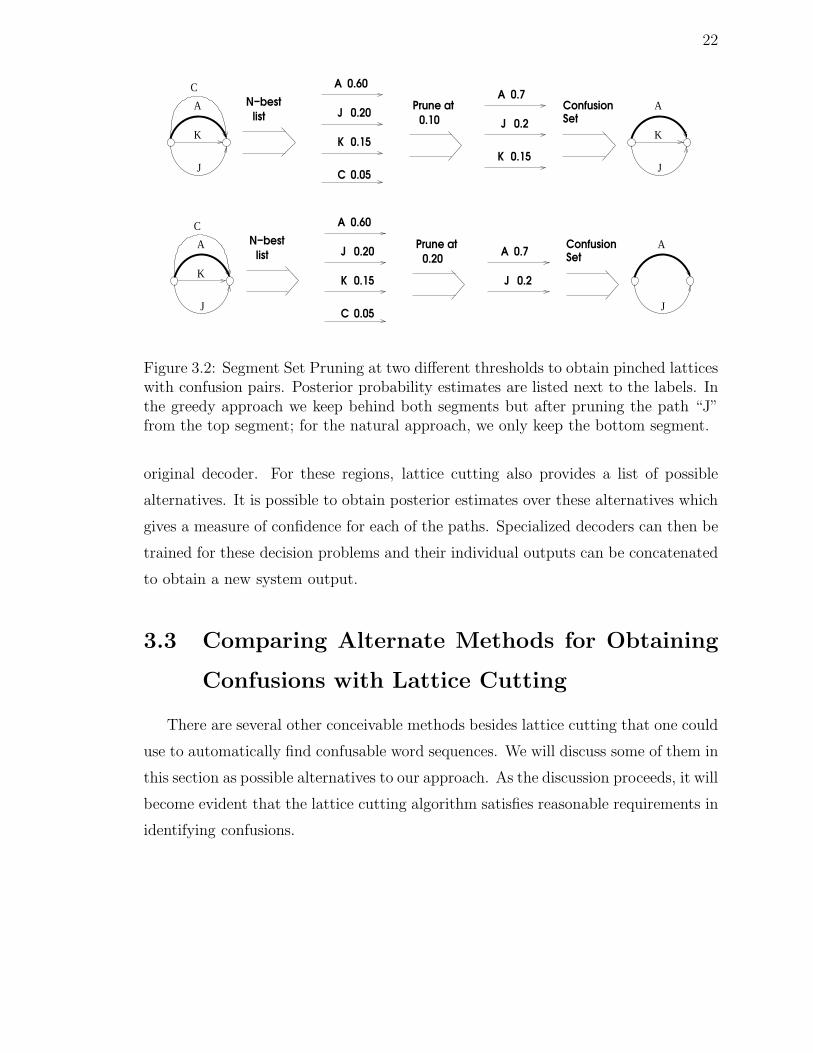
3.2 Segment Set Pruning at two different thresholds to obtain pinched lat-tices with confusion pairs. Posterior probability estimates are listednext to the labels. In the greedy approach we keep behind both seg-ments but after pruning the path “J” from the top segment; for thenatural approach, we only keep the bottom segment. . . . . . . . . . 22

3.3 Locating training instances when the truth of the decoded data is avail-able. Erroneous segments #3 and #6 can be taken as training data. . 26

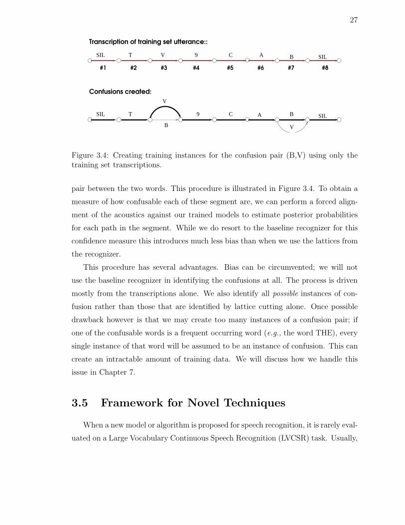
3.4 Creating training instances for the confusion pair (B,V) using only thetraining set transcriptions. . . . . . . . . . . . . . . . . . . . . . . . . 27

4.1 A hyperplane classifier over two class data. The two classes are indi-cated by circles and squares. . . . . . . . . . . . . . . . . . . . . . . . 31

4.2 An original two-dimensional linearly non-separable problem becomesseparable in three dimensions after applying a feature transformationζ(·). . . . . . . . . . . . . . . . . . . . . . . . . . . . . . . . . . . . . 34

x

4.3 Graphical solution for a classical formulation of a soft-margin SVMformulation. The top plot shows the loss associated with training dataas a function of its distance from the margin; the bottom left gives ameasure of the sparseness of the final solution; the bottom right givesthe potential function . . . . . . . . . . . . . . . . . . . . . . . . . . . 36

4.4 Graphical solution for Probabilistic Kernel Logistic Regression. Thetop plot shows the loss associated with training data as a function ofits distance from the margin; the bottom left gives a measure of thesparseness of the final solution; the bottom right gives the potentialfunction, the Shannon Entropy function. Note the loss function neverreaches 0; hence the solution is not sparse. . . . . . . . . . . . . . . . 37

4.5 Graphical solutions for binary GiniSVM. The top plot shows the lossassociated with training data as a function of its distance from themargin; the bottom left gives a measure of the sparseness of the finalsolution; the bottom right gives the potential function, a quadraticfunction. Note the loss function is 0 for zi > 4γ; hence sparsity can becontrolled. . . . . . . . . . . . . . . . . . . . . . . . . . . . . . . . . . 39

5.1 A pinched lattices with the models on each path of a confusion pairtagged with the index of the corresponding confusion pair. . . . . . . 46

5.2 Kernel Map K( Ψ(Oi; θ), Ψ(Oj; θ) ) for the linear kernel over two classdata. . . . . . . . . . . . . . . . . . . . . . . . . . . . . . . . . . . . . 53

5.3 Kernel Map K( Ψ(Oi; θ), Ψ(Oj ; θ) ) for tanh kernel over two class data. 53

6.1 WERs for different PLMMI seeded SVM code-breaking systems as theglobal SVM trade-off parameter (C) is varied. . . . . . . . . . . . . . 72

6.2 WERs for the sequence of incremental PLMMI SVM code-breaking sys-tems. Origin refers to no confusion pairs considered, i.e., the PLMMIHMM system. X-axis = 1 refers to the system that considers onlythe confusion pair with the most of amount of training data; X-axis= 2 refers to the system that considers the two confusion pairs withthe most amount of training data; and so on. The blue Y-axis givesthe WER of various systems. The green Y-axis gives the count of thetraining instances for the SVM that has been added to the IncrementalPLMMI SVM code-breaking system. . . . . . . . . . . . . . . . . . . 74

7.1 Examples of different kinds of confusions. Each path is labeled withboth the word and its phonetic sequence. left: a homonym confusionpair. center: a non-homonym confusion pair. right: a phonetic confu-sion pair. . . . . . . . . . . . . . . . . . . . . . . . . . . . . . . . . . . 80

7.2 Code Breaking schematic for automatic speech recognition. The figureshows some examples of he specialized decoders that can be used incode-breaking. . . . . . . . . . . . . . . . . . . . . . . . . . . . . . . . 81

xi

7.3 Labeling identified binary confusions as CPCOR or CPERR and asMAPCOR or MAPERR. The MAP hypothesis in the pinched latticeis shown in bold. Segments #2 and #6 are MAPCOR and CPCOR;segment #3 is MAPERR and CPERR; segment #7 is MAPERR andCPCOR. . . . . . . . . . . . . . . . . . . . . . . . . . . . . . . . . . . 84

7.4 Error counts over individual confusion pairs. The confusion pair withtheir indices are listed in Table 7.6 . . . . . . . . . . . . . . . . . . . 92

8.1 Phonetic Transformation Regression Tree. The symbols are elaboratedin Table 8.2 . . . . . . . . . . . . . . . . . . . . . . . . . . . . . . . . 104

xii

List of Tables

6.1 Performance of various baseline HMM systems. ML: Baseline HMMstrained under the ML criterion; MMI: The ML HMMs are trainedusing MMI; PLMMI: The MMI HMMs were MMI trained on the MMIpinched lattices. The restriction in the last column is that the confusionpairs allowed are only the 50 most frequently observed ones in the MMIcase. . . . . . . . . . . . . . . . . . . . . . . . . . . . . . . . . . . . . 65

6.2 Frequent confusion pairs found by lattice cutting on the MMI lattices.Indices provided indicate the rank of the confusion pair as determinedfrom their number of errors identified on the test set; more number ofidentified errors implies a higher rank. From V. Doumpiotis et al. [22]. 66

6.3 Measuring the approximations induced by restricting pinched test setlattices to binary confusion problems. ‘50 frequent binary confusionsLER’ refers to to LER after restricting the pinched lattice to the 50most frequently occurring confusion found on the MMI training set lat-tices. ‘Binary confusions LER’ is the LER after restricting the pinchedlattice to all identified binary confusions. . . . . . . . . . . . . . . . . 67

6.4 WERs of various HMM and SVM code-breaking systems. ML: BaselineHMMs trained under the ML criterion; MMI: The ML HMMs aretrained using MMI; PLMMI: The MMI HMMs were MMI trained onthe MMI pinched lattices . . . . . . . . . . . . . . . . . . . . . . . . . 69

6.5 WERs for PLMMI seeded SVM code-breaking systems with trade-offparameter tuning. . . . . . . . . . . . . . . . . . . . . . . . . . . . . . 72

6.6 Piecewise Rule for choosing the trade-off parameter (C) through thenumber of training observations (N). . . . . . . . . . . . . . . . . . . 72

6.7 WERs of various HMM and SMBR-SVM systems. A: Baseline HMMstrained under the ML criterion; B: The HMMs from A are trained usingMMI; C: The HMMs from A were trained using Forward-Backward ononly the confusable segments; D: The HMMs from A were cloned andtagged as illustrated in Fig. 3.1, d and were trained using Forward-Backward on only the confusable segments; . . . . . . . . . . . . . . . 75

xiii

6.8 WERs of HMM systems with and without MLLR transforms; SMBR-SVM systems were trained in the Score-Space of the transformed models 78

7.1 LER of various lattices prior to and after pruning. . . . . . . . . . . . 837.2 Lattice Pinching and LER. The average number of hypotheses per

segment set, number of distinct segment sets, and total number ofsegment sets after posterior-based pruning. Threshold 0.0 correspondsto Fig. 3.1 c with NULL hypotheses discarded. . . . . . . . . . . . . . 86

7.3 Ratio of #CPCOR/#CPERR segments and #MAPERR/#MAPCORsegments for the confusion pairs observed at least 100 times in the 25hour test set. . . . . . . . . . . . . . . . . . . . . . . . . . . . . . . . 87

7.4 To demonstrate that the optimal pruning threshold for the ‘natural’approach to finding confusions can be chosen robustly over an held outset. . . . . . . . . . . . . . . . . . . . . . . . . . . . . . . . . . . . . . 87

7.5 Performance of various models when evaluated on the ‘confusion pairstraining set’ created to train MMI word level HMMs. The hypothesisof each model for each segment set was taken to be the word that wasassigned an higher likelihood. No language model information is usedduring this evaluation. . . . . . . . . . . . . . . . . . . . . . . . . . . 90

7.6 Confusion Pairs and their Indices listed in Figure 7.4 . . . . . . . . . 93

8.1 Baseform and Surface Acoustic Model Performance. . . . . . . . . . . 1028.2 Base Acoustic Classes Used to Construct Phonetic Transformation Re-

gression Classes. Classes are based on vowel manner and place of ar-ticulation: front, central, back, high, middle, low. . . . . . . . . . . . 103

8.3 Pronunciation Modeling Performance Showing Phone Error Rate Re-duction as Phonetic Transformation Regression Classes are Introduced. 105

xiv

1

Chapter 1

Introduction

Automatic Speech Recognition (ASR) is a sequential pattern recognition problem

in which the patterns to be hypothesized are words while the evidence presented to

the recognizer is the acoustics of a spoken utterance. Given an acoustic signal, a

speech recognizer attempts to classify it as the sequence of words that was spoken.

The goal of the speech recognizer is to guess as many of the words correctly

as possible. However due to various factors like inaccurate modeling assumptions,

insufficient training data, mismatched training and test conditions, an ASR system

may not correctly hypothesize all the spoken words. If these erroneous hypotheses can

be reliably identified and characterized, we can then develop special purpose decoders

that work only to fix these specific errors made by the original recognizer. By the

use of these decoders we can attempt a refinement of the first-pass hypothesis so as

to improve overall recognition performance.

This dissertation presents and develops this idea of what can be done to identify

and correct the errors that occur consistently in the output of the speech recognizer.

We term this technique of decoding as code-breaking.

Code-breaking is an approach that attempts to improve upon the performance of

the original decoder rather than replace it. It is a divide-and-conquer technique where

we first identify regions where a decoder is weak and then use specialized decoders to

fix those problematic regions. The regions of uncertainty or confusion are found in

an unsupervised manner and this appears as a list of alternative hypotheses for each

2

[I],[???],[apples]]

high confidenceregion outputs

First−passDecoder

HypothesisSpace Identification

of "difficult"regions

output FinalHypothesis

SpecializedDecoder

low confidenceregions

I love apples

[love]

Measurements

I love apples

Spectral

[love,dove,live]

I live applesI love applesI dove apples

Figure 1.1: Code Breaking for ASR.

region. This identification process reduces a complex sequential pattern classification

problem into a sequence of smaller independent problems. The idea behind code-

breaking is to attack these smaller problems using special-purpose decoders trained

specifically to find the true hypothesis in the confusable regions.

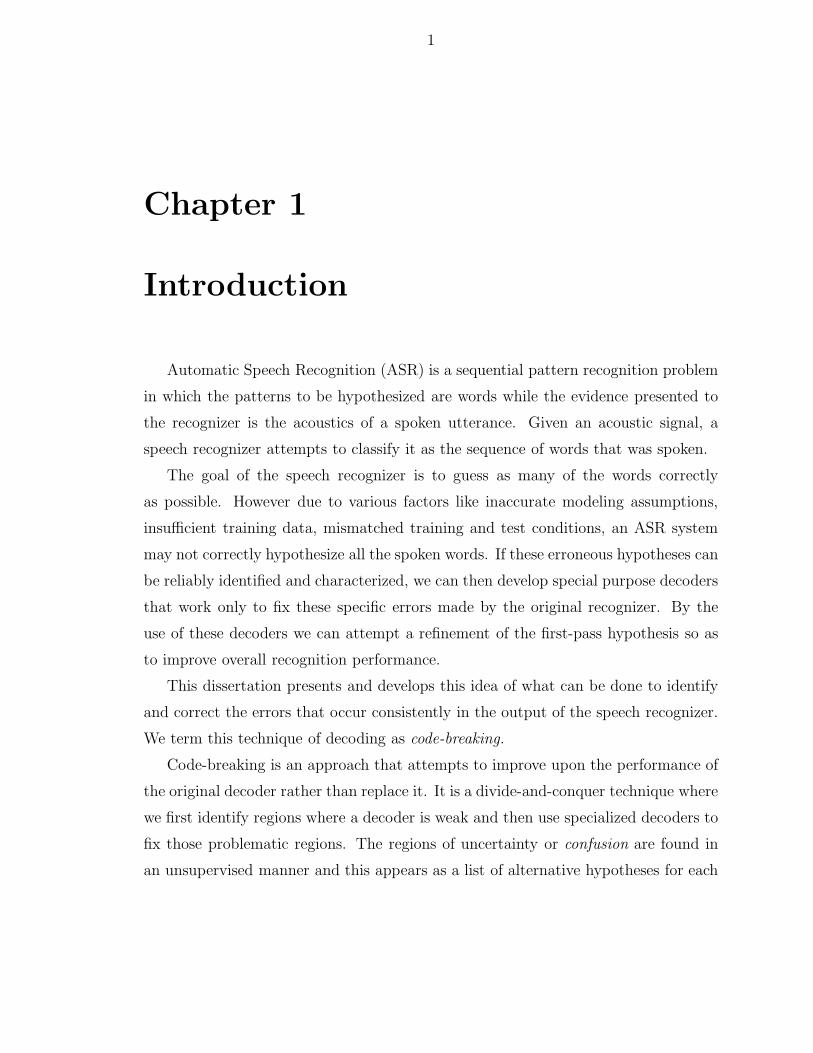
A schematic of the code-breaking framework applied to speech recognition is given

in Figure 1.1. We only process those segments that are “difficult” for the first-pass

decoder. The other segments are simply retained and concatenated in place with the

outputs of the specialized decoder to obtain the final system output.

Code Breaking also entails locating relevant training data for the specialized de-

coders. We take the relevant data to be instances in the training data that can help

in distinguishing between the confusable words.

There have been previous research efforts which can be interpreted as code-

breaking. We will review them in Section 5.8 and discuss how they differ from the

framework that we propose.

This dissertation mainly focuses on two-word confusion problems, e.g., DOG vs.

BOG, BEAR vs. BARE, etc. We will investigate the use of Support Vector Ma-

chines (SVMs) as our specialized decoders; however, any other binary classifier can

also be used. While multiclass decoders are also suitable for code-breaking, the aim

of this thesis is to demonstrate the idea for binary problems. We consider extending

3

the approach to multi-class problems to be a separate research issue.

1.1 Motivation

There are several reasons to want to apply code-breaking for ASR. Since the

original recognizer has little a priori knowledge, it will have to distinguish between

the words (say) DOG and BOG and between the words DOG and DOT. Now assume

that the recognizer has eliminated DOT as a choice but is unable to choose between

DOG and BOG. Code-breaking makes it possible to use a specialized decoder capable

of distinguishing between ‘DOG’ and ‘BOG’ without having to account for ‘DOT’.

Without the analysis of the first-pass hypothesis, such a simple choice would not have

been possible for the original speech recognizer.

It is also arguable that the optimal decoder for a binary recognition problem is

one that is specialized to distinguish between the two words only. The original speech

recognizer is no longer the optimal decoder since it was built to distinguish between

all possible words sequences that can be spoken. Code-breaking makes it possible to

use a specialized decoder capable of making a more informed choice.

While discriminative training procedures have been successfully developed for ASR

systems, it is possible that they do so at the cost of one word sequence over the

other. Code-breaking attempts to uniformly reduce the errors within confusable word

sequences.

When identifying regions of confusions, we will transform ASR from a complex

recognition task into a sequential problem composed of smaller independent classifi-

cation tasks. We can now apply simple decoders to each these smaller classification

problems. Thus code-breaking provides a framework for incorporating models that

might not otherwise be appropriate for continuous speech recognition.

ASR systems are also used in tasks like indexing oral archives where the goal is to

provide easy access to a large collection of audio data. These tasks are mainly driven

through the identification of keywords in the collection. Code-breaking can identify

confusions involving these keywords so as to make the ASR system robust to errors

involving these keywords.

4

1.2 Organization of Thesis

The rest of the chapters are organized as follows:

• Chapter 2 gives an overview of Hidden Markov Modeled based ASR systems

and introduces speech recognition terminology used in the thesis.

• Chapter 3 describes the algorithm we use to identify regions of confusions and

the methods we use to find relevant training data for building specialized de-

coders.

• Chapter 4 reviews the Support Vector Machine (SVM), a large-margin classifier

and the GiniSVM, a variant of the SVM which we will use to obtain posterior

probability estimates.

• Chapter 5 discusses the issues involved in applying GiniSVMs in ASR and

code-breaking in particular. We also give a review of prior work that can be

interpreted as code-breaking and the usage of SVMs in ASR.

• Chapter 6 presents experiments over a small vocabulary corpus that is designed

to validate the idea of code-breaking.

• Chapter 7 demonstrates the feasibility of code-breaking on a large vocabulary

corpus. We will also discuss the sparsity issue that has to be addressed to obtain

further improvements on large vocabulary tasks.

• Chapter 8 presents clustering in the context of pronunciation modeling as a

means of capturing consistent acoustic changes.

• Chapter 9 lists the contributions of this thesis and gives directions for future

work.

5

Chapter 2

An Overview of Automatic Speech

Recognition

This chapter gives an overview of Automatic Speech Recognition (ASR) systems.

We will also introduce terminology that will be used through the rest of this thesis.

Let a speaker who says a word string W = w1 · · ·wN generate a waveform A. The

goal of the the ASR system is then to recover the word string W from A.

This speech waveform A is first digitized by sampling at a high frequency; typically

44.1KHz for microphone audio or 8KHz for telephone channel speech. The sampled

waveform is then converted into a T -length observation vector sequence O = o1 · · ·oT

by the Acoustic Processor or the front-end of the speech recognizer.

The maximum a posteriori (MAP) recognizer can then be formulated as follows [2,

81, 53]: choose the most likely word string (W ) given the acoustic data:

W = argmaxW∈W

P (W |O), (2.1)

where W represents all possible word strings. Using Bayes rule we can write,

W = argmaxW∈W

P (O|W )P (W )

P (O). (2.2)

Since the search in Equation (2.2) is independent of O, it follows the recognizer can

search according to the rule

W = argmaxW∈W

P (O|W )P (W ). (2.3)

6

We will now briefly discuss the individual components of a MAP recognizer.

2.1 Acoustic Modeling

To compute P (O|W ) we employ an acoustic model, usually a Hidden Markov

Model (HMM). L. Rabiner and B-H Juang [81] and F. Jelinek [53] give a detailed

description of the HMM methodology used in speech recognition. An HMM is defined

by

• a finite state space 1, 2, · · · , S;

• an output space O, usually RD;

• transition probabilities between states, aij = P (st = i|st−1 = j); and

• output distributions for states, bj(·) = P (ot|st = j).

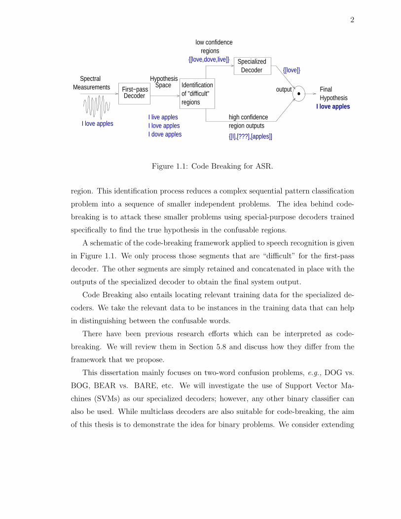
An example of an HMM borrowed from the HTK manual [27] is illustrated in Fig-

ure 2.1.

a12 a23 a34 a 45

a22 a33 a44

1 2 3 4 5

a24 a35

b2( ) b3( ) b4( )

a13

Figure 2.1: Example of an Hidden Markov Model (from the HTK manual [27]).

The HMM representation of a hypothesis W is a concatenation of HMMs that

represent smaller units. Each word w is represented by a sequence of phones and

7

A

W

O

q

B

u

Word sequence give an example to illustrate

eh g z ae m p ax l

ae.3ae.2ae.1

Time sequence of states

State sequence

Phone sequence

Time sequence of

Acoustic signal

acoustic observationvectors

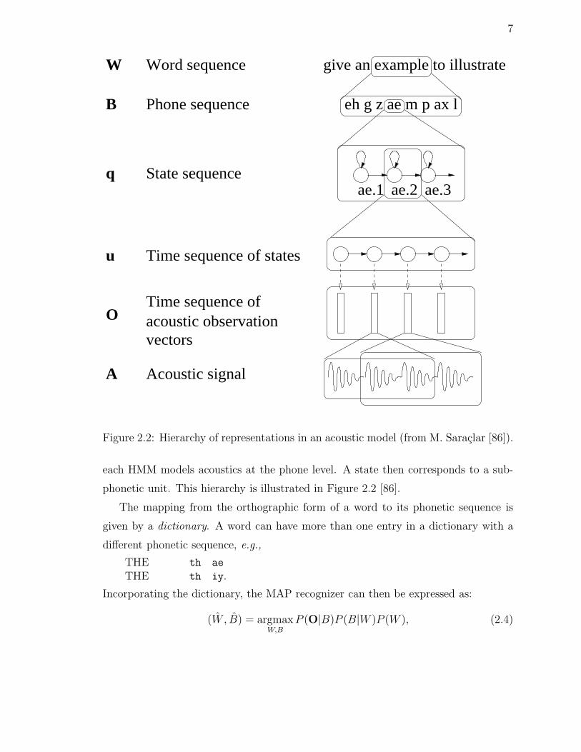
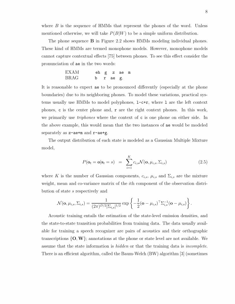
Figure 2.2: Hierarchy of representations in an acoustic model (from M. Saraclar [86]).

each HMM models acoustics at the phone level. A state then corresponds to a sub-

phonetic unit. This hierarchy is illustrated in Figure 2.2 [86].

The mapping from the orthographic form of a word to its phonetic sequence is

given by a dictionary. A word can have more than one entry in a dictionary with a

different phonetic sequence, e.g.,

THE th ae

THE th iy.

Incorporating the dictionary, the MAP recognizer can then be expressed as:

(W , B) = argmaxW,B

P (O|B)P (B|W )P (W ), (2.4)

8

where B is the sequence of HMMs that represent the phones of the word. Unless

mentioned otherwise, we will take P (B|W ) to be a simple uniform distribution.

The phone sequence B in Figure 2.2 shows HMMs modeling individual phones.

These kind of HMMs are termed monophone models. However, monophone models

cannot capture contextual effects [75] between phones. To see this effect consider the

pronunciation of ae in the two words:

EXAM eh g z ae m

BRAG b r ae g.

It is reasonable to expect ae to be pronounced differently (especially at the phone

boundaries) due to its neighboring phones. To model these variations, practical sys-

tems usually use HMMs to model polyphones, l-c+r, where l are the left context

phones, c is the center phone and, r are the right context phones. In this work,

we primarily use triphones where the context of c is one phone on either side. In

the above example, this would mean that the two instances of ae would be modeled

separately as z-ae+m and r-ae+g.

The output distribution of each state is modeled as a Gaussian Multiple Mixture

model,

P (ot = o|st = s) =

K∑

i=1

ci,sN (o, µi,s, Σi,s) (2.5)

where K is the number of Gaussian components, ci,s, µi,s and Σi,s are the mixture

weight, mean and co-variance matrix of the ith component of the observation distri-

bution of state s respectively and

N (o, µi,s, Σi,s) =1

(2π)D/2|Σi,s|1/2exp

−1

2(o − µi,s)

⊤Σ−1i,s (o − µi,s)

.

Acoustic training entails the estimation of the state-level emission densities, and

the state-to-state transition probabilities from training data. The data usually avail-

able for training a speech recognizer are pairs of acoustics and their orthographic

transcriptions O,W; annotations at the phone or state level are not available. We

assume that the state information is hidden or that the training data is incomplete.

There is an efficient algorithm, called the Baum-Welch (BW) algorithm [3] (sometimes

9

called the Forward-Backward (FB) algorithm) that enables the estimation of model

parameters given incomplete training data under the Maximum-Likelihood (ML) cri-

terion. Baum-Welch is an instance of the Expectation Maximization (EM) technique.

The EM algorithm is an iterative technique. We first assign initial values to the

model parameters. Then we maximize the expected log-likelihood (known as the

auxiliary function) where the expectation is over the hidden variables. The expec-

tation (E-step) is calculated with the current model parameters. Then we maxi-

mize (M-step) the auxiliary function with respect to the model parameters to obtain

new estimates. We can now iterate with these new estimates. The EM algorithm

guarantees not to decrease the likelihood assigned to the training data. A. P. Demp-

ster et al. [21] give a formal treatment of the EM algorithm.

If θ is the set of the current parameters for the HMMs, the auxiliary function is

given by

Q(θ, θ′) =∑

q∈Q

P (s|O,W; θ) logP (O, s|W; θ′) (2.6)

where Q are all state sequences that can represent W and θ′ are the newly estimated

parameters of the HMM.

The training data is usually speech obtained from hundreds of speakers; the re-

sultant system is therefore termed as a Speaker-Independent (SI) system. During

testing when speech from an unseen speaker has to be decoded, to reduce mismatch,

a linear transform (A) is applied to the parameters of the SI models to better match

the speech from the test speaker. These Speaker-Dependent (SD) models are usually

obtained by transforming the means of the Gaussians alone. The new observation

densities are given by

P (o|s) =

K∑

i=1

ci,s

(2π)D/2|Σi,s|1/2exp

−1

2(o − Aµi,s)

⊤Σ−1i,s (o − Aµi,s)

. (2.7)

The most popular transform used is the Maximum Likelihood Linear Regression (MLLR)

transform [60]. This transform (A) is computed so as to increase the likelihood as-

signed by the SD models to the hypothesis of the SI system. Referring to Equation 2.6,

the parameters to be re-estimated are now the transforms A, the acoustics O are from

the test speaker and the W are now the transcriptions obtained from the SI system.

10

The ML paradigm attempts to increase the likelihood assigned to the training

data by the corresponding model. There are discriminative training frameworks that

besides increasing the training set likelihood under the corresponding models also

attempts to lower the likelihood assigned by competing model sequences. Maximum

Mutual Information (MMI) [74, 43, 102] is one such criterion which tries to maximize

the mutual information between the training word sequences W and the observation

sequences O. Formally MMI attempts to estimate parameters as

θ′ = argmaxθ

logP (O|W )P (W )

∑

W ′ P (O|W ′)P (W ′). (2.8)

2.2 Language Modeling

P (W ), the prior over the word strings that can be hypothesized is estimated by a

language model [51]. It is usually an n-gram model as,

P (W ) =M∏

i=1

P (wi|wi−1wi−2 · · ·wi−n+1) (2.9)

where M is the number of words in W . Typically, the language model used is a

bigram or a trigram language model where n = 2 or n = 3 respectively.

2.3 ASR Decoding, Lattices, and Posterior Prob-

ability Estimates

Since the acoustic model is HMM-based and the language model can be repre-

sented by a Markov model, the joint model can be thought of as a large HMM. MAP

decoding according to Equation 2.4 involves searching this huge network and deter-

mining the most likely path given the acoustic observations. Usually a form of Viterbi

decoding [96] is used to obtain the MAP hypothesis.

The token passing model [84] is one such formulation of the Viterbi algorithm.

As we traverse the large HMM structure, we associate a token with each state j at

time t (a brute force implementation requires the replication of the the huge network

11

structure for each time instant t). Among other information, the token contains the

likelihood of the most likely path that ends in state j while observing all observations

until time t. The token also has back pointers that give the most likely state sequence

that reached j. This token is then passed on to all states that connect to j and

the log-likelihood of the token is updated with the corresponding transition and the

observation likelihoods. If there are multiple tokens that arrive at a state, we only

keep the highest scoring token. Once all the speech (or all the acoustic observations)

has been processed we then use the trace back information of the token on the best

scoring state and recover the most likely word sequence.

We can also keep behind all tokens at each state that have a likelihood within a

predetermined window of the top scoring token for that state. The trace back infor-

mation then produces a compact representation of the set of most likely hypotheses.

Such a representation is called a lattice (see Figure 2.3, top). We can then generate

the N most likely hypotheses according to the speech recognizer. Such a list is called

an N-best list.

Each link l in the lattice represents a single word hypothesis. Associated with

each link are also the start and end times of the word hypothesis and the acoustic

and language model scores for that word. We would like to associate a measure of

a-posteriori probability to each link in the lattice; this will give us both a means of

comparing two links in a lattice and a measure of confidence of the system in its

hypothesis.

We follow the framework introduced by Wessel et al. [101] and then developed by

Evermann and Woodland [30]. The link posterior probability γ(l|O) is defined as the

ratio of the sum of the likelihoods of all paths passing through l to the likelihood of

the observed data. Formally,

γ(l|O) =

∑

QlP (W,O)

P (O)(2.10)

where W is a hypothesis in the lattice, Ql are all paths passing through l, and P (O)

is approximated by the sum of the likelihoods of all the paths in the lattice. The

summation over Ql can be efficiently performed with the FB algorithm over the links

of the lattice links using its start and end times.

12

A number of links in the lattice can represent multiple hypotheses of a word at

a given time instant. This is due to different acoustic segmentations and also due to

different word contexts. One method of obtaining a word posterior distribution for a

given time frame is to add the posterior probabilities of all links that span the given

frame and correspond to the word [101]. Thus each word in a hypothesis from the

lattice can be associated with a posterior probability estimate for each time instant

t. For convenience we omit O in the notation of the posterior word probability as

γw(t).

Each link representing a word in the lattice can be broken down into a sequence

of links representing HMM states. With a similar analysis just described (replacing

the words with the states), we can define posterior probability estimates γi,s(t) of

the state s of the ith HMM at time t. The posterior probabilities of the component

mixtures at time t are then estimated as

γi,s,j(t) = γi,s(t)N (ot, µi,s,j, Σi,s,j)

∑

x N (ot, µi,s,x, Σi,s,x)(2.11)

where j is the mixture component index of state s under the ith HMM. Mixture

posterior probabilities can readily be estimated when we have a single hypothesis W

for an acoustic observation sequence O. In this case, we first estimate the state-level

posterior probabilities using the FB algorithm and then use Equation 2.11.

Given a observation string O = o1, o2, · · · , oT and a word string W , forced align-

ment or viterbi alignment refers to finding the most likely state sequence that could

have generated the observations along with the time segments corresponding to each

state. This alignment can be obtained by using the Viterbi algorithm.

A standard decoding framework for state-of-the-art LVCSR systems is lattice

rescoring. Say we use a monophone based HMM speech recognizer to generate a

set of lattices over the test set. The links in the lattices have besides the start and

end times and the language model scores, the acoustic scores from the monophone

based HMMs. Now assume we want to make use of a triphone based acoustic model (it

may have been too computationally expensive to use the triphone-based model and

generate a first-pass lattice). We can now estimate new acoustic scores for each link

with the triphone HMMs using the time segments given in the lattice and then re-

13

TODAYARE YOU ALL

First−Pass lattice:

</s>

</s>

</s>

MAP hypothesis:

NOWHELLO ARE YOU ALL TODAY

Truth:

HOWHELLO

ARE

ARE

WELL TO

HELLO

WELL

YOU

YOU

ALL

TODAYO

NOW

NOW

YOU

TODAY

TO

DAY

DAY

ARE

HOW

HOW

Figure 2.3: Example of a Lattice, the MAP hypothesis and the true transcription.The arcs in the most likely hypothesis have been highlighted.

place the lattice acoustic scores with the newly estimated ones. We can now search

within the lattice to obtain a different and possibly better MAP hypothesis. The

method of rescoring a lattice by replacing the acoustic model scores is called acoustic

rescoring while replacing the language model scores and rescoring is called language

model rescoring.

2.4 Evaluation Criteria

ASR systems are usually evaluated under the Word Error Rate (WER) criterion.

The WER is defined to be the ratio of the number of recognition errors to the number

of words in the truth. The number of recognition errors is the minimum number of

insertions, deletions and substitutions required to obtain the truth from the recognizer

output. This measure also called the Levenshtein distance [61] can be efficiently

calculated using dynamic programming techniques. The truth is usually taken to be

human transcriptions; humans listen to the speech closely and write down what they

think was spoken. In the example given in Figure 2.3, since there is a substitution

error between HOW and NOW, the WER is 1/6 ≈ 18%.

14

Another performance measure is the Phone Error Rate (PER). Its is defined sim-

ilarly as the WER but the transcriptions are compared at the phone level. The PER

is especially of interest in the context of pronunciation modeling, where we attempt

to model variations of speech at the phone level.

The quality of lattices produced by a speech recognizer can be measured by the

Lattice Error Rate (LER). It is the WER of the lattice hypothesis with lowest WER

with respect to the truth. The brute force method of obtaining the LER would be

to expand the lattice into an exhaustive list of individual hypotheses; computing the

WER for each of them; and finding the minimum value among the WERs. However

in practice, the LER is found via an efficient lattice-based search. In the example in

Figure 2.3, the LER is 0%.

15

Chapter 3

Identification of Confusions

The previous chapter gave a brief overview of an Automatic Speech Recogni-

tion (ASR) system. Given a sequence of acoustic observations, the system searches

through a network of allowed hypotheses, and finds the most likely hypothesis that

could have generated the input acoustics. As the system searched through the net-

work the recognizer could have encountered regions of acoustics where the alternatives

to the most likely word were nearly nearly just as likely. We will refer to these re-

gions where the recognizer is not sure about its guess as ‘confusable regions’ and the

sets of words and phrases that were assigned comparable probability estimates as

‘confusions’.

Our first step in code-breaking is to analyze the lattices generated by a speech

recognizer to locate the confusable regions and identify the different confusions that

the speech recognizer encountered. This step will be done in an ‘fair’ and unsupervised

manner, i.e., we will not access the true transcriptions of the decoded speech.

In this chapter, we will first describe an algorithm called lattice pinching that can

transform a first-pass lattice into a sequence of smaller sub-lattices. These sub-lattices

will contain words and phrases which can be considered as likely alternatives to the

MAP hypothesis. The original models (say the acoustic or language) are weak over

these regions in that the system was unable to pick a clear winner from among the

competing hypotheses; these sub-lattices essentially define the regions of weaknesses

that remain after the first recognition pass. We will discuss the relationship between

16

the first-pass lattice and the sub-lattices along with some of the issues involved in

identifying regions of confusion in this way. We will also discuss alternate methods,

not pursued here, for identifying such confusions of a speech recognizer.

Once we have identified the confusions, which we also refer to as sub-problems,

we want to resolve them with specialized decoders. For building these kinds of de-

coders we need to obtain training data that can help in distinguishing the confused

words. We will discuss methods of choosing appropriate training data under various

scenarios, e.g., depending on the availability of held-out data, availability of reference

transcriptions, etc. We will conclude this chapter by pointing out the new framework

that lattice cutting allows for evaluation of novel techniques in speech recognition.

To make the presentation clearer, the illustrations in this chapter will be from a

corpus [72] whose vocabulary is alphabets and digits alone. Thus the letter B and

the number 8 will be among the words to be recognized by the system.

3.1 Lattice Cutting

For our purposes, lattice cutting [42, 57] is a procedure that segments an input

lattice into sub-lattices. These sub-lattices when concatenated together can represent

all the paths in the original lattice. More importantly, the sub-lattices contain words

and phrases which can be considered as likely alternatives to the MAP hypothesis.

Figure (3.1, top) shows a lattice output by a decoder. The primary hypothesis is

highlighted in bold. Figure (3.1,bottom) gives the sub-lattices that have been con-

catenated together.

Lattice Cutting takes as input a lattice (L) with posterior probabilities on the

links, a primary hypothesis (W ), and a loss function l(·, ·) between two word strings.

Our description of the lattice cutting algorithm is in terms of Finite State Machine

operations; a brief tutorial is given in the Appendix A. Further details of the algo-

rithm can be obtained from the paper by V. Goel et al. [42]. We closely follow their

description.

1. Lattice to Primary Hypothesis Path Alignment. The first step is to obtain all

17

ε

A

A A V

B

K

J4

OHSIL SIL9

C

K(3,sub,1)

A(3,.,0) 9(4,.,0)

V(7,.,0)

SIL(1,.,0) OH(2,.,0)

4(2,sub,1)

J(3,sub,1) 9(4,.,0)

9(4,.,0)SIL(8,.,0)

A(6,sub,1)

C(3,sub,1)

OH

C

A

J

4

9

9

K

SIL

SIL8V

AA

First−pass lattice:

Aligned Lattice:

Pinched Lattice:

Alignment

CollapsingAlignedSegments

9

(5,del,1)8(6,.,0)

8

A(5,.,0)

ε

#1 #2 #3 #4 #5 #6 #7 #8

Lattice−to−path

EB

B

SIL(8,.,0)B(7,sub,1)

E(7,ins,1)

B(7,sub,1)

SIL(8,.,0)

B

SIL

E

SIL

Figure 3.1: Lattice Segmentation. a: First-pass lattice with MAP path in bold;b: Alignment of the lattice to the MAP path under the Levenshtein distance; thelink labels give the word hypothesis, segment index, edit operation, and its alignmentcost; ǫ denotes a NULL link; c: Collapsed segment sets; The numbers the bottomgive the indices of the collapsed segment set

18

possible alignments between the reference word string and the lattice. For

this, we create a simple transducer (T ) that has links representing alignments

between all words (not paths) in the lattice to the words in the reference hy-

pothesis. We obtain a new lattice by the composition L T W that specifies

all possible string-edit operations that can transform any possible path in the

original lattice to the primary hypothesis.

2. Least cost alignment between all paths to the reference path. We then obtain the

best alignment for each path in the lattice to the reference path. This process

implies enumerating all possible alignments of each path in the lattice to the

reference hypothesis and then choosing the best among them. This is simply

intractable. However there is an approximate efficient algorithm [41, 57] that

transforms the original lattice to a form (see Figure 3.1,middle) that contains

all the information needed to find the best alignments of every word string to

the reference hypothesis W . The information contained for every word in the

lattice consists of the identity of the word in the primary hypothesis it is aligned

to, the edit-operation involved in the alignment and the cost of alignment.

3. Lattice Pinching. Using the alignment information we can then collapse word

strings that align with the same reference string segment. This transforms the

original lattice into a form in which all paths in the lattice are represented as

alternatives to the words in the reference string W (see Figure 3.1,bottom). We

refer to this collapsing of lattice segments as pinching and the resultant lattice

as a pinched lattice.

The pinched lattice contains a sequence of collapsed segments, or segment sets.

They have been indexed in Figure (3.1,c). Some of the segments (e.g., #4) are

regions where the reference hypothesis does not align with any other path. These

indicate high-confidence regions where the recognizer was sure about its hypothesis.

Other segments (e.g., #2, #3, #6, and #7), where the primary hypothesis has many

alternatives indicate low confidence regions. These low-confidence regions can be

viewed as ASR sub-problems that the original decoder could not solve with a high

19

degree of confidence. Note that while the hypothesis space L has been segmented,

we emphasize the observed acoustics O remain unsegmented.

The process of lattice cutting did not remove any paths from the lattice; any

path in the original lattice (Figure (3.1,top)) remains in the pinched lattice (Fig-

ure (3.1,bottom)). This ensures that the Lattice Error Rate (LER) is less than or

equal to that of the first-pass lattice. In fact new paths are usually added; the LER

of the pinched lattice is typically lower compared to the original lattice.

Some of the segment sets can contain NULL links. In Figure 3.1, segment set #5

has a NULL (ǫ) link. These are contributed by lattice paths that are shorter than

the reference.

Lattice cutting does not disrupt the structure of the original lattice. Since the

alignment was done at the lattice-path level rather than at the word level, we ensured

that the relative order of the links was not changed. We can still perform lattice

rescoring of the pinched lattices with refined acoustic or language models to obtain

improvements.

Unless otherwise stated, our loss function l(·, ·) will be the Levenshtein loss. In

this case, the segment sets defined will be under a loss function that does not use the

scores on the links of the original lattice. However, if we inspect Figure (3.1,top) and

Figure (3.1,middle), we see that they have identical word sequences. Therefore we

can get the acoustic and language model scores for the aligned lattice by composing

it with the original lattice. This will enable us to define posterior distributions over

the segment sets obtained in Figure (3.1,bottom). We will be using these posterior

probability estimates extensively to decide on what ASR sub-problems we want to

resolve. For the collapsed lattices, the posterior probability of a link l will be the sum

of the posterior probabilities of all links in the original lattice that are now represented

by l.

The lattice segmentation procedure, in its current implementation [42], leads to

loss of time information present in the nodes of the original lattice. To obtain start

and end times of a link with respect to a path in the pinched lattice we can perform

forced alignment against the acoustic data.

The Levenshtein loss function is insensitive to the identity of the word, i.e., the

20

loss for different words is always the same irrespective of the words being compared.

This is meaningful if we are interested in confusions of the decoder in general and

we can set l(G,Z) = l(C,Z). However, if we are only interested in locating specific

confusions like those that arise from voicing, we would set l(G,Z) > l(C,Z).

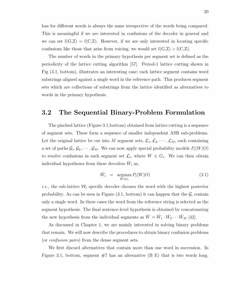
The number of words in the primary hypothesis per segment set is defined as the

periodicity of the lattice cutting algorithm [57]. Period-1 lattice cutting shown in

Fig (3.1, bottom), illustrates an interesting case; each lattice segment contains word

substrings aligned against a single word in the reference path. This produces segment

sets which are collections of substrings from the lattice identified as alternatives to

words in the primary hypothesis.

3.2 The Sequential Binary-Problem Formulation

The pinched lattice (Figure 3.1,bottom) obtained from lattice cutting is a sequence

of segment sets. These form a sequence of smaller independent ASR sub-problems.

Let the original lattice be cut into M segment sets, L1,L2, · · · ,LM , each containing

a set of paths G1,G2, · · · ,GM . We can now apply special probability models Pi(W |O)

to resolve confusions in each segment set Li, where W ∈ Gi. We can then obtain

individual hypotheses from these decoders Wi as,

Wi = argmaxWǫGi

Pi(W |O) (3.1)

i.e., the sub-lattice Wi specific decoder chooses the word with the highest posterior

probability. As can be seen in Figure (3.1, bottom) it can happen that the Gi contain

only a single word. In these cases the word from the reference string is selected as the

segment hypothesis. The final sentence-level hypothesis is obtained by concatenating

the new hypothesis from the individual segments as W = W1 · W2 · · · WM [42].

As discussed in Chapter 1, we are mainly interested in solving binary problems

that remain. We will now describe the procedures to obtain binary confusion problems

(or confusion pairs) from the dense segment sets.

We first discard alternatives that contain more than one word in succession. In

Figure 3.1, bottom, segment #7 has an alternative (B E) that is two words long.

21

When these alternate paths are removed, it gives groups of single word hypothesis.

The presence of a NULL requires answering the question “Should the word in the

primary hypothesis be deleted?”. Since the MAP hypothesis could easily contain a

wrongly inserted word or phrase, this is clearly a problem of interest and specialized

detectors could be built to attack it. But we mostly ignore this problem; we simply

discard the NULL links. The effect of this approximation can be measured by the

increase the LER.

The segment sets obtained after the above operations (dropping successive words

and epsilons) can still be very dense. Towards obtaining binary problems, we follow

one of two pruning strategies:

1. The greedy approach. We simply keep the two most likely paths (the MAP

hypothesis and the most likely alternative) in each segment set. This approach

is greedy is the sense that we attempt to consider as many binary confusions as

possible.

2. The natural confusions approach. As we shall see in Chapter 7, many of the

alternatives will have very small posterior probability estimates and can be dis-

carded without catastrophic degradation in the LER. We can thus use posterior

based pruning schemes to reduce the number of likely alternatives. Figure 3.2

illustrates pruning at a couple of thresholds. After pruning, some segment sets

become “natural” binary confusions, i.e., these segments have only two paths

each with a posterior probability estimate greater than the pruning thresh-

old (Figure 3.2, bottom). Other segment sets with more than two paths can

remain. In these cases, we simply prune back to the one-best.

We are now finally left with a pinched and pruned lattice that is a sequence of

segments that either have just a single word or have pairs of confusable words, shown

in Figure 3.3, top. These segment sets contain the words labels and the estimated

word posteriors on each path. G(1) and G(2) refer to the individual words. We can

now use binary pattern classifiers to choose from these two words.

In summary, lattice cutting converts ASR into a sequence of smaller, independent

sub-problems. These smaller regions of acoustic confusion indicate weaknesses of the

22

A

N−best

list

A 0.7

0.2J

K 0.15

C 0.05

Prune at

0.10

ConfusionSet

J

A

A 0.60

0.20J

K 0.15

K

J

C

A

K

N−best

list A 0.7

0.2JK 0.15

C 0.05

Prune at

0.20

ConfusionSet

J

A

A 0.60

0.20J

K

J

C

Figure 3.2: Segment Set Pruning at two different thresholds to obtain pinched latticeswith confusion pairs. Posterior probability estimates are listed next to the labels. Inthe greedy approach we keep behind both segments but after pruning the path “J”from the top segment; for the natural approach, we only keep the bottom segment.

original decoder. For these regions, lattice cutting also provides a list of possible

alternatives. It is possible to obtain posterior estimates over these alternatives which

gives a measure of confidence for each of the paths. Specialized decoders can then be

trained for these decision problems and their individual outputs can be concatenated

to obtain a new system output.

3.3 Comparing Alternate Methods for Obtaining

Confusions with Lattice Cutting

There are several other conceivable methods besides lattice cutting that one could

use to automatically find confusable word sequences. We will discuss some of them in

this section as possible alternatives to our approach. As the discussion proceeds, it will

become evident that the lattice cutting algorithm satisfies reasonable requirements in

identifying confusions.

23

3.3.1 A Priori Confusions

The dictionary of an ASR system lists the words and their phonetic representa-

tion that is modeled by the HMMs. Word pairs that are within a small number of

edit-string operations of each other can be assumed to be confusable. Consider the

dictionary entries for the words DOG and BOG:

DOG d ao g

BOG b ao g.

The phonetic representation of these words differs by only one substitution of the first

phone. It seems reasonable to assume that these words as confusable.

We can then proceed to find relevant training data to obtain examples to build a

decoder to tell the words apart. However such a listing only gives a-priori confusions

and is not directly related to the acoustic properties of the HMMs or the linguistic

properties of the language model. Most of the confusions we hypothesize will not

occur during decoding. We want to focus instead on word sequences that are truly

confusable in practice for the recognizer rather than all those that are potentially

confusable. This suggests that the process of identification has to be driven from the

regions of confusion that occur in the decoding process.

3.3.2 Errors from the Decoding Output

The decoding output is a single hypothesis with posterior probability estimates

of how likely the decoder finds the words in the hypothesis. Words with higher

estimates indicate high confidence of the recognizer in its output. However a low

estimate implies that the recognizer could not make a sure guess. This can indicate

a region of confusion where the recognizer is unable to find the truth and instead

chooses a wrong path in the lattice. It is also possible that the truth is an OOV

token and could not be hypothesized by the system at all.

To identify confusions we need to find what word sequences were confused with the

low-confidence word sequences. It would be ideal to have what was really spoken, i.e.,

the true transcriptions, as alternates in these low-confidence regions. If the specialized

decoders then picked the alternative paths, this would be exactly what code-breaking

24

was meant to do: identify flaws that remain after the training of the decoder and then

rectify them. Since we do not assume any access to the transcriptions for the test set,

we need to find a method to generate reasonable alternatives for the low-confidence

regions.

3.3.3 Obtaining Confusions from a Lattice

The lattices output by the recognizer naturally provide alternate paths to the

one-best hypothesis. While we are not assured that any one of the alternate paths

is the truth, for a well-trained ASR system the LER of the lattices produced will be

much lower than the WER of the 1-best path. Thus if we were able to use all the

alternate paths collectively there is scope for significant improvements.

Identifying confusions directly from lattices is not trivial. Typical lattices in large

vocabulary tasks are very dense and extremely complex; it is not uncommon to have

thousands of links for a time frame.

A reasonable path to consider for generating alternatives to the low-confidence

regions in the one-best path is the second-most likely path. Unfortunately, it is often

the case the second best path will be different from the best path in just one word.

This does not give us enough variability to identify all confusions in an utterance. An

alternative approach is to generate an N-best list and attempt to identify confusions

from aligning each hypothesis to the one-best path. Some of the problems in using

N-best lists are (i) listing out enough number of alternatives to cover a substantial

portion of the lattice becomes intractable, (ii) there are a large number of duplicate

alternatives with different time segmentations and (iii) identifying confusions becomes

inefficient when the size of the list increases.

We need to process the lattice and transform the lattice for highlighting the prob-

lems the decoder encountered by the decoder. We would like any transformation of

the lattice for locating confusion be such that it (i) keeps the structure of the original

lattice. By this we mean that the relative order of the words must be preserved; for

any pair of words in the initial lattice such that the second word is a successor of the

first word, the same relative order must be preserved in the transformed lattice. This

25

is so that rescoring the transformed lattices with the specialized decoder is sensible;

otherwise this can result in catastrophic WER degradation. We also want to ensure

that (ii) we do not lose any paths in the original lattice. This restriction is more

obvious; we want the LER to remain low. We would like to do this alignment and

comparison of posteriors over all paths in the lattice. As we saw early on in this

chapter, lattice cutting [42] does perform alignment of all paths in the lattice against

a word string and satisfies the two conditions that are mentioned here.

3.4 Obtaining Relevant Training data for the Bi-

nary Classifiers

We have so far discussed the identification of confusions in a test set in an un-

supervised manner. Once we have identified the confusions or the sub-problems, we

want to resolve them with specialized decoders. For building these kinds of decoders

we need to obtain training data that can help in distinguishing the confused words.

In contrast with the methods discussed so far, this process need not be unsupervised;

we can access the true transcriptions of the training data. We will now discuss the

two methods we used.

1. Matched confusions. The first method we used was to repeat the entire process

of identifying confusions on the test set for the training set as well. We generated

lattices on the training set; cut the lattices; and then pruned them. This process will

identify confusions (that remain) in the data over which the recognizer was trained on.

We used the true transcription of the training set as the reference hypothesis for the

lattice cutting procedure. Since the lattice cutting procedure does not require scores

on the paths, we can still create segment sets. For pruning to get binary confusions,

we simply kept behind the truth and the most probable hypothesis for each segment.

One issue with this method is that cutting and pruning the training set lattices

can be quite computationally intensive. A less intensive approach would be to simply

process the one-best hypothesis obtained by decoding the training set and take all

errors as confusions to be resolved. Since we have the transcriptions of the training

26

4

OH AASIL SIL

OH ASIL SILK A

truth:

pinched lattices with confusion pairs:

#5 #8#6#3 #4 #7#1 #2

A

J

9

9

8 V

B

B

Figure 3.3: Locating training instances when the truth of the decoded data is avail-able. Erroneous segments #3 and #6 can be taken as training data.

set we can align both these hypotheses and any errors in the recognized output will

be highlighted by costs in the alignment. An example is illustrated in Figure 3.3.

We can see that K and A have been misrecognized as A and 8 in segments #3 and

#6 respectively. The segments can then be used as training data for the specialized

decoder to help fix these errors. However, this approach is suboptimal since we

identify errors rather than confusions; we will end up with much less training data.

There are also some bias issues with using the output of the recognizer over the

training data in identifying confusions; the decoder could have learnt the training

data well enough that it will not make as many or even the same kind of errors as

on unseen data. To handle the kind of errors problem, we can use a held-out set.

Finding as many instances of confusions to be able to perform reliable training of

the specialized decoder then becomes a problem; its rare to have enough transcribed

held-out data comparable to the size of the training data itself.

2. Transcription based confusions. The second method we used was an even less

intensive approach that does not use the outputs of a recognizer at all; we only use

the transcriptions of the training set. Suppose we have identified a confusion between

the words w1 and w2 after analysis of the test set lattices. We simply assume every

instance of the word w1 in the training set is an instance of confusion with w2 and

vice-versa. For every utterance with the word w1 we created an instance of a confusion

27

A

SIL

CSIL SIL

V

B

9

V

BT

T C SILA

#5 #8#6#3 #4 #7#2

9 B

Transcription of training set utterance::

Confusions created:

V

#1

Figure 3.4: Creating training instances for the confusion pair (B,V) using only thetraining set transcriptions.

pair between the two words. This procedure is illustrated in Figure 3.4. To obtain a

measure of how confusable each of these segment are, we can perform a forced align-

ment of the acoustics against our trained models to estimate posterior probabilities

for each path in the segment. While we do resort to the baseline recognizer for this

confidence measure this introduces much less bias than when we use the lattices from

the recognizer.

This procedure has several advantages. Bias can be circumvented; we will not

use the baseline recognizer in identifying the confusions at all. The process is driven

mostly from the transcriptions alone. We also identify all possible instances of con-

fusion rather than those that are identified by lattice cutting alone. Once possible

drawback however is that we may create too many instances of a confusion pair; if

one of the confusable words is a frequent occurring word (e.g., the word THE), every

single instance of that word will be assumed to be an instance of confusion. This can

create an intractable amount of training data. We will discuss how we handle this

issue in Chapter 7.

3.5 Framework for Novel Techniques

When a new model or algorithm is proposed for speech recognition, it is rarely eval-

uated on a Large Vocabulary Continuous Speech Recognition (LVCSR) task. Usually,

28

the evaluation is done on a small corpus or is compared to an extensively simplified

baseline system. The reason for this recourse is the sheer complexity involved in im-

plementing a new technique in an LVCSR task. Consider the case of a new pattern

classifier that seems to show promise in complex binary classification tasks. Attempt-

ing to use such a classifier directly in an LVCSR task is very daunting. One method

to evaluate the new classifier in LVCSR tasks is to reduce the complex ASR task into

a sequence of binary tasks.

The techniques described in this chapter can be used to define sub-problems within

a LVCSR task. Lattice cutting can reduce ASR into a sequence of independent smaller

decision problems. We can specify the complexity of the tasks using the periodicity of

the cutting and with pruning. To use simple binary pattern classifiers, we can create

a sequence of binary decision problems. The characteristics of the sub-problems can

be chosen by using different loss function during the lattice-to-word-string alignment.

We can also assess the value that a new model or algorithm can add to an existing

state-of-the-art recognizer. Suppose that the new technique is really powerful in dis-

tinguishing a particular class of words, e.g., words with voiced and unvoiced features.

Lattice cutting can then be used to find out how often the baseline system encounters

confusions between these kinds of words. This will give a measure on how much the

new technique can possibly help in performance on top of the existing recognizer.

In the following chapters we will show Support Vector Machines, a class of com-

paratively simple classifiers, can be gainfully used to improve the performance of an

ASR system in this framework.

29

Chapter 4

Kernel Regression Methods

Chapter 2 described how Hidden Markov Models (HMMs) are used in Automatic

Speech Recognition (ASR). The basic idea was to attempt to learn the generative

process (P (A|W )) and then use Bayes Rule to find argmaxW P (A|W )P (W ). In con-

trast, large margin classifiers attempt to find decision boundaries directly rather than

through estimating a probability distribution over the training data.

We first briefly review the most popular large margin classifier, the Support Vec-

tor Machine (SVM) [93]. One drawback of the basic SVM is that its raw outputs

are unnormalized scores and have to transformed to obtain conditional probability

estimates. We then present an unified framework called Probabilistic Kernel Regres-

sion [49] that subsumes SVMs. Normalized scores can be generated from some large

margin classifiers under this framework. Finally, we present the GiniSupport Vector

Machine [15], an approximation to the Kernel Logistic Regression (KLR) [50]. Unlike

KLR, the GiniSVM produces both sparse solutions and has a quadratic optimization

function. We will conclude this chapter with a brief discussion justifying the use of

large margin classifiers.

As discussed in Chapter 1, we are primarily interested in using binary classifiers

as our specialized decoders. Hence we will restrict the discussion in this chapter to

binary classifiers alone; multi-class classifiers will not add value to our discussions.

30

4.1 Support Vector Machines

Support Vector Machines (SVMs) [93] are pattern recognizers that classify data

without making any assumptions about the underlying process by which the observa-

tions were generated. In their basic formulation SVMs are binary classifiers. Given a

data sample to be classified, the SVM will assign it as belonging to one of two classes.

An SVM is defined by a hyperplane. The points x that lie on the hyperplane

satisfy φ · x + b = 0, where φ is the normal to the hyperplane (we use φ rather than

the conventional w to represent the normal to the hyperplane to avoid confusion with

representing words as w), b/||φ|| is the perpendicular distance from the hyperplane

to the origin and ||φ|| is the Euclidean norm of φ.

Let xili=1 be the training data and yil

i=1 be the corresponding labels, where

xi ∈ Rd and yi ∈ −1, +1. We assume that the training data is drawn independently

from a fixed distribution P (x, y) defined over RD × +1,−1.

The goal of the SVM algorithm is to find the hyperplane that discriminates the

data from the two classes. The measure of discrimination is formalized by the “margin

width”, defined as the distance from the separating hyperplane to the positive and

the negative samples. If the distance from the hyperplane to the closest training data

point is normalized to unity, the margin is given by 2/||φ||. Figure 4.1 illustrates the

situation described.

Assuming that the training data are separable by the hyperplane (Figure 4.1

without the two error vectors), the optimal hyperplane has the maximum margin and

classifies the training data correctly. In other words, we can locate the hyperplane if

we minimize 12||φ||2 under the following constraints:

xi · φ + b ≥ +1 ∀yi = +1

xi · φ + b ≤ −1 ∀yi = −1

or combining them together,

yi(xi · φ + b) − 1 ≥ 0 ∀i. (4.1)

When the training data is not separable, we would like to relax the constraints for

those points that have been incorrectly classified. This is usually done by introducing

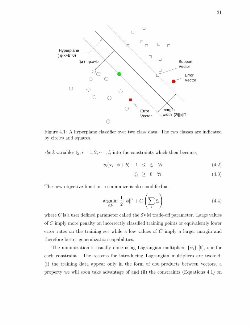
31

.x+b=0)

marginwidth

Hyperplane

SupportVector

(

ErrorVector

ErrorVector (2/||φ||)

f(x)= φ.x+b

φ

Figure 4.1: A hyperplane classifier over two class data. The two classes are indicatedby circles and squares.

slack variables ξi, i = 1, 2, · · · , l, into the constraints which then become,

yi(xi · φ + b) − 1 ≤ ξi ∀i (4.2)

ξi ≥ 0 ∀i (4.3)

The new objective function to minimize is also modified as

argminφ,b

1

2||φ||2 + C

(

∑

i

ξi

)

(4.4)

where C is a user defined parameter called the SVM trade-off parameter. Large values

of C imply more penalty on incorrectly classified training points or equivalently lower

error rates on the training set while a low values of C imply a larger margin and

therefore better generalization capabilities.

The minimization is usually done using Lagrangian multipliers αi [6], one for

each constraint. The reasons for introducing Lagrangian multipliers are twofold:

(i) the training data appear only in the form of dot products between vectors, a

property we will soon take advantage of and (ii) the constraints (Equations 4.1) on

32

the training data will be replaced with constraints on the Lagrangian multipliers

themselves, which are much easier to handle.

The primal Lagrangian [34] is given by

argminφ,b

1

2||φ||2 + C

∑

i

ξi −∑

i

αi(yi(xi · φ + b) − 1 + ξi) −∑

i

λiξi (4.5)

where λi are Lagrangian multipliers to enforce the positivity of ξi. Maximizing the

primal w.r.to φ, b and ξ under first order conditions we get,

φ =∑

i

αiyixi (4.6)

∑

i

αiyi = 0 (4.7)

C − αi − λi = 0 (4.8)

and

λiξi = 0 (4.9)

Equation 4.6 shows that the solution φ is determined only by the points whose αi 6= 0.

These are points that lie on the hyperplane or whose zi ≤ 1. They are termed support

vectors in the sense that the SVM solution depends on them. So, if we want sparse

solutions, we want to have αi = 0 for a substantial number of training data.

Substituting these solutions in the primal gives the dual problem [34]:

argmaxαi

∑

i

αi −1

2

∑

ij

αiαjyiyj(xi · xj) (4.10)

subject to

0 ≤ αiC, (4.11)∑

i

αiyi = 0 (4.12)

Note that in the dual only the αis need be estimated. The SVM obtained as the

solution is called the soft-margin SVM classifier.

The solution for the hyperplane is given by

φ =∑

i

αiyixi (4.13)

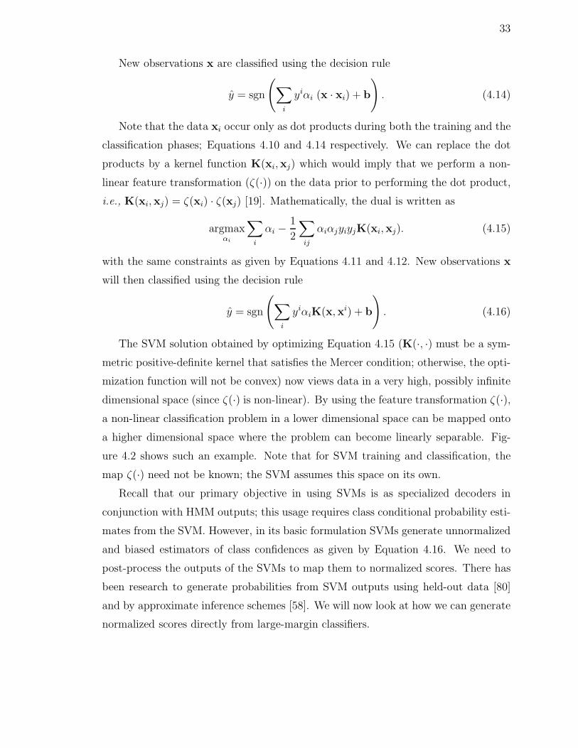
33

New observations x are classified using the decision rule

y = sgn

(

∑

i

yiαi (x · xi) + b

)

. (4.14)

Note that the data xi occur only as dot products during both the training and the

classification phases; Equations 4.10 and 4.14 respectively. We can replace the dot

products by a kernel function K(xi,xj) which would imply that we perform a non-

linear feature transformation (ζ(·)) on the data prior to performing the dot product,

i.e., K(xi,xj) = ζ(xi) · ζ(xj) [19]. Mathematically, the dual is written as

argmaxαi

∑

i

αi −1

2

∑

ij

αiαjyiyjK(xi,xj). (4.15)

with the same constraints as given by Equations 4.11 and 4.12. New observations x

will then classified using the decision rule

y = sgn

(

∑

i

yiαiK(x,xi) + b

)

. (4.16)

The SVM solution obtained by optimizing Equation 4.15 (K(·, ·) must be a sym-

metric positive-definite kernel that satisfies the Mercer condition; otherwise, the opti-

mization function will not be convex) now views data in a very high, possibly infinite

dimensional space (since ζ(·) is non-linear). By using the feature transformation ζ(·),

a non-linear classification problem in a lower dimensional space can be mapped onto

a higher dimensional space where the problem can become linearly separable. Fig-

ure 4.2 shows such an example. Note that for SVM training and classification, the

map ζ(·) need not be known; the SVM assumes this space on its own.

Recall that our primary objective in using SVMs is as specialized decoders in

conjunction with HMM outputs; this usage requires class conditional probability esti-

mates from the SVM. However, in its basic formulation SVMs generate unnormalized

and biased estimators of class confidences as given by Equation 4.16. We need to

post-process the outputs of the SVMs to map them to normalized scores. There has

been research to generate probabilities from SVM outputs using held-out data [80]

and by approximate inference schemes [58]. We will now look at how we can generate

normalized scores directly from large-margin classifiers.

34

ζ (•)

Figure 4.2: An original two-dimensional linearly non-separable problem becomes sep-arable in three dimensions after applying a feature transformation ζ(·).

4.2 Probabilistic Kernel Regression Framework

In the primal SVM formulation presented above (Equation 4.5), we used slack

variables to increase the cost of each misclassified data point. These slack variables

can be viewed as a loss incurred by erroneously classifying the corresponding training

data point. We can formalize this notion by introducing a loss function g(·) [12] which

would be a function of z = yi(w · x + b), the absolute distance of vector xi from the

hyperplane. We can now rewrite the primal cost function (L) as

argminφ,b

1

2|φ|2 + C

∑

i

g(zi) (4.17)

where g(·) is a non-negative convex loss function. Taking derivatives of Equation 4.17

with respect to φ and b and applying first order conditions we have,

∂L

∂w= φ + C

∑

i

g′(zi)yixi = 0 (4.18)

∂L

∂b= C

∑

i

g′(zi)yixi = 0 (4.19)

where g′(·) is the derivative of g(·).

Let

αi = −Cg′(zi). (4.20)

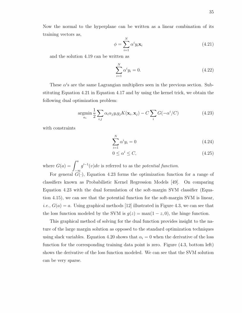
35

Now the normal to the hyperplane can be written as a linear combination of its

training vectors as,

φ =N∑

i=1

αiyixi (4.21)

and the solution 4.19 can be written as

N∑

i=1

αiyi = 0. (4.22)

These αis are the same Lagrangian multipliers seen in the previous section. Sub-

stituting Equation 4.21 in Equation 4.17 and by using the kernel trick, we obtain the

following dual optimization problem:

argminαi

1

2

∑

i,j

αiαjyiyjK(xi,xj) − C∑

i

G(−αi/C) (4.23)

with constraints

N∑

i=1

αiyi = 0 (4.24)

0 ≤ αi ≤ C, (4.25)

where G(a) =

∫ a

−∞

g′−1(v)dv is referred to as the potential function.

For general G(·), Equation 4.23 forms the optimization function for a range of

classifiers known as Probabilistic Kernel Regression Models [49]. On comparing

Equation 4.23 with the dual formulation of the soft-margin SVM classifier (Equa-

tion 4.15), we can see that the potential function for the soft-margin SVM is linear,

i.e., G(a) = a. Using graphical methods [12] illustrated in Figure 4.3, we can see that

the loss function modeled by the SVM is g(z) = max(1 − z, 0), the hinge function.

This graphical method of solving for the dual function provides insight to the na-

ture of the large margin solution as opposed to the standard optimization techniques

using slack variables. Equation 4.20 shows that αi = 0 when the derivative of the loss

function for the corresponding training data point is zero. Figure (4.3, bottom left)

shows the derivative of the loss function modeled. We can see that the SVM solution

can be very sparse.

36

g(zi)

zi = yi.(φ.xi+ b)

1

1

g’(zi)

zi

-1

1

C

Cα

i

G

Figure 4.3: Graphical solution for a classical formulation of a soft-margin SVM for-mulation. The top plot shows the loss associated with training data as a function ofits distance from the margin; the bottom left gives a measure of the sparseness of thefinal solution; the bottom right gives the potential function

Due to their use of the kernel trick, Probabilistic Kernel Regression Models still

retain several advantages of the original SVM formulation. In addition if the potential

function is chosen appropriately, we will see that they can also generate normalized

scores.

The common choice for the potential function is the Shannon entropy function,

H(a) = −a log a − (1 − a) log(1 − a). Substituting this form of H(a) as G(a) in

Equation 4.23 gives the the dual corresponding to binary kernel logistic regression [50]:

argminαi

1

2

∑

i,j

αiαjyiyjK(xi,xj) + C∑

i

( αi/C ) log( αi/C )

+ C∑

i

( 1 − (αi/C) ) log( 1 − (αi/C) )(4.26)

with constraints 4.24 and 4.25. Once again, using graphs (shown in Figure 4.4)

we can see that the corresponding loss function being modeled is given by g(z) =

log(1 + exp(−z)). This is the maximum likelihood loss function corresponding to the

37

g(zi)

zi = yi.(φ.xi + b)

1

-1

g’(zi)

zi

-1

C ln2

Cα

i

G

Figure 4.4: Graphical solution for Probabilistic Kernel Logistic Regression. The topplot shows the loss associated with training data as a function of its distance fromthe margin; the bottom left gives a measure of the sparseness of the final solution;the bottom right gives the potential function, the Shannon Entropy function. Notethe loss function never reaches 0; hence the solution is not sparse.

binary Kernel Logistic Regression probability model

P (+1|x) =1

1 + exp( −f(x) )(4.27)

where f(x) =∑

i yiαiK(xi,xj). The bias of the hyperplane has been subsumed as an

extra dimension of the features. Thus we can obtain normalized scores directly from

Kernel Logistic Regression.

Figure (4.4, bottom left) shows the derivative of the loss function g′(z). We see

that g′(z) is not zero for any value of z. Hence all training points contribute to

the solution; there is no sparsity. For large training sets, this can easily turn out

to be prohibitive due to memory and run-time constraints. Also, while the dual

optimization problem is both continuous and convex, it is not quadratic; rather it is

logistic. This precludes the use of fast quadratic programming (QP) techniques.

We would like to choose an appropriate potential function that can give normalized

scores while at the same have the properties of the original SVM: sparse solutions

and a quadratic optimization function.

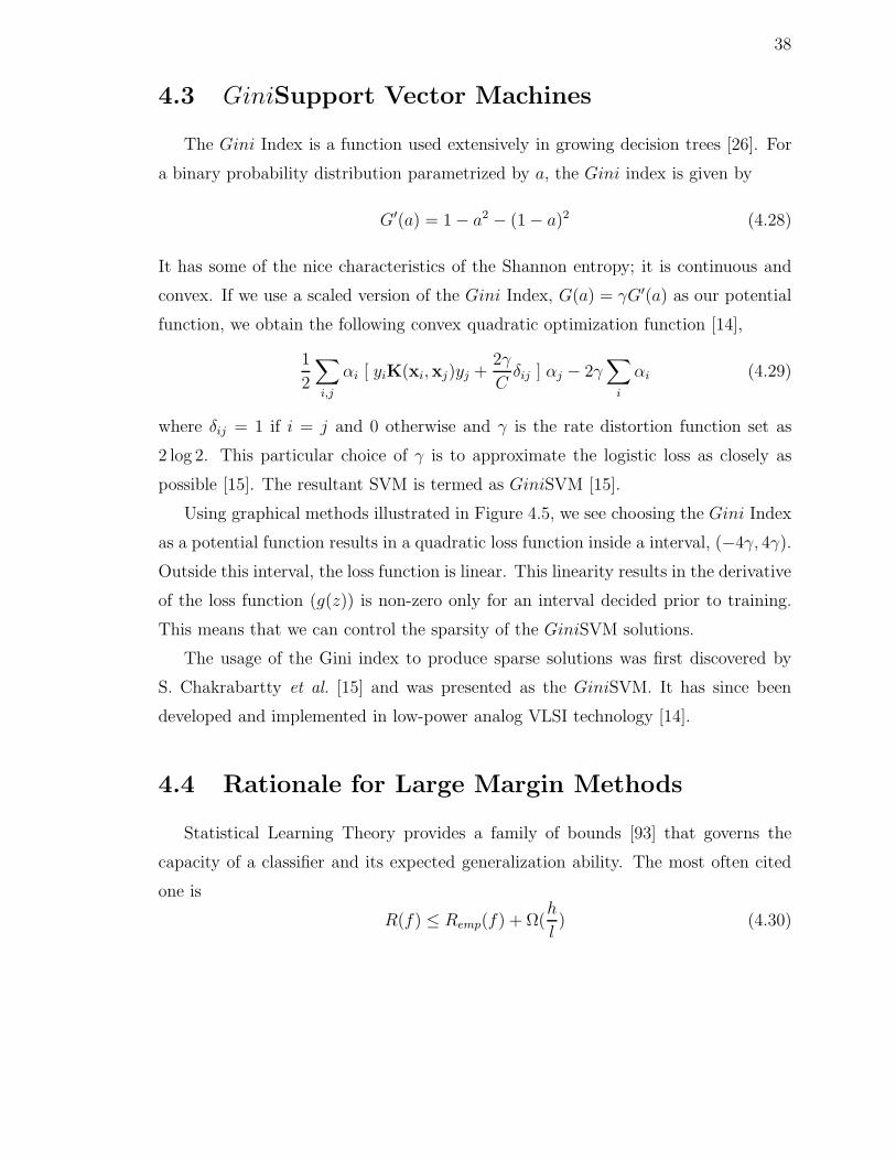
38

4.3 GiniSupport Vector Machines

The Gini Index is a function used extensively in growing decision trees [26]. For

a binary probability distribution parametrized by a, the Gini index is given by

G′(a) = 1 − a2 − (1 − a)2 (4.28)

It has some of the nice characteristics of the Shannon entropy; it is continuous and

convex. If we use a scaled version of the Gini Index, G(a) = γG′(a) as our potential

function, we obtain the following convex quadratic optimization function [14],

1

2

∑

i,j

αi [ yiK(xi,xj)yj +2γ

Cδij ] αj − 2γ

∑

i

αi (4.29)

where δij = 1 if i = j and 0 otherwise and γ is the rate distortion function set as

2 log 2. This particular choice of γ is to approximate the logistic loss as closely as

possible [15]. The resultant SVM is termed as GiniSVM [15].

Using graphical methods illustrated in Figure 4.5, we see choosing the Gini Index

as a potential function results in a quadratic loss function inside a interval, (−4γ, 4γ).

Outside this interval, the loss function is linear. This linearity results in the derivative

of the loss function (g(z)) is non-zero only for an interval decided prior to training.

This means that we can control the sparsity of the GiniSVM solutions.

The usage of the Gini index to produce sparse solutions was first discovered by

S. Chakrabartty et al. [15] and was presented as the GiniSVM. It has since been

developed and implemented in low-power analog VLSI technology [14].

4.4 Rationale for Large Margin Methods

Statistical Learning Theory provides a family of bounds [93] that governs the

capacity of a classifier and its expected generalization ability. The most often cited

one is

R(f) ≤ Remp(f) + Ω(h

l) (4.30)

39

g(zi)

zi = yi.(φ.xi+ b)-4γ

g’(zi)

zi

-1

γC

Cα

G4γ

4γ

Figure 4.5: Graphical solutions for binary GiniSVM. The top plot shows the lossassociated with training data as a function of its distance from the margin; the bottomleft gives a measure of the sparseness of the final solution; the bottom right gives thepotential function, a quadratic function. Note the loss function is 0 for zi > 4γ; hencesparsity can be controlled.

where R(f) is the expected error rate on unseen test data of a classifier f drawn from

a family S, Remp(f) is the empirical error rate, Ω is a monotonic function, h is a

complexity parameter and l is the size of the training set.

The second summand in Equation 4.30 gives a measure of the structural risk de-

termined by the complexity or the power of the classifier family S. Among classifiers

with the same performance on the training set, the classifier with the least complexity

has the best generalization ability. The complexity of a family of classifiers is formal-

ized as the VC-dimension. For the family of hyperplane classifiers, the complexity

parameter is bounded from above as

h ≤ min

(

R2

∆2, n

)

+ 1 (4.31)

where n is the dimension of the hyperplane space, R is the radius of the sphere

containing all the the training data points and ∆ is the margin of separation between

the two classes for the family S. Thus among hyperplane classifiers that classify the

training data correctly, the hyperplane with the largest margin generalizes the best.

40

It is of interest to compare the primal objective function of the SVM (Equation 4.4)

to Equation 4.30. We repeat the former for convenience.

argminφ,b

1

2||φ||2 + C

(

∑

i

ξi

)

We can see that the first term corresponds to inverse of the margin width while the

second term to the empirical error. Thus we see the SVM algorithm attempts to

jointly minimize the empirical risk and the structural risk. During implementation,

the empirical risk is first implicitly fixed by setting the SVM trade-off parameter (C)

and then the structural risk is minimized by choosing the hyperplane with the largest

margin. This margin maximization is the power of SVMs; without it, SVMs will

overfit the data in the high dimensional feature space.

It might be worth pointing out that Equation 4.30 represents the worst-case sce-

nario; the test data is assumed to be as mismatched as possible in terms of perfor-

mance of the classifier family S.

41

Chapter 5

Code-Breaking with GiniSupport

Vector Machines

The previous chapter discussed large-margin classification methods and reviewed

how the GiniSupport Vector Machine (GiniSVM). We reviewed how the GiniSVM

uses large margin techniques to perform classification while at the same time gives

normalized scores as its outputs. These normalized scores are then interpreted as

posterior probability estimates.

This chapter will discuss the modeling issues involved when using SVMs in speech

recognition in general and also in the code-breaking framework. We will first discuss

score-spaces, the features obtained to train the GiniSVMs. We will also show that

GiniSVMs trained in these score-spaces is an approximate solution for the parameters

of the logistic regression problem of estimation of a posterior distribution over the

hypotheses of a segment set. We will briefly discuss the kernels that we found were

useful in obtaining discriminatory information in the score-spaces and also discuss

some of the practical issues involved in estimating sufficient statistics for each segment

set. We will finally lay out the steps involved in incorporating GiniSVMs in the code-

breaking framework. In the course of presenting this approach, we do discuss issues

and factors that led to the final modeling strategy, and in Section 5.8 we review and

compare this modeling approach to other prior work in this area.

42

5.1 Motivation and Challenges

Support Vector Machines (SVMs) are discriminative pattern classifiers that have

shown remarkable performance [8, 24, 59] in static pattern classification tasks (by

static we mean that the observations of the patterns to be classified are of a fixed

dimension, d). Some of these tasks include handwriting recognition [59] and text

classification. They show good generalization performance due to both the “large-

margin” property of the defining hyperplane and the hyperplane being determined

by a small number of training data points.

As we saw in Chapter 2 speech recognition systems are based on Hidden Markov

Models (HMMs), a generative methodology for pattern classification. By using SVMs

in speech recognition it is hoped that some of the beneficial properties of SVMs can

be realized in ASR.

There are however some significant challenges in applying SVMs to Automatic

Speech Recognition (ASR). We focus here on two of them:

1. Variable length observations. SVMs are static classifiers; a data sample to be

classified must belong to an input space (Rd). Speech recognition is inherently

a dynamic pattern recognition problem. Two utterances of the same word

from the same speaker still cannot be expected to be of equal length. The

variable length observations from the speech signal have to be mapped into

fixed dimensional space if SVMs can be used at all.

2. Sequential multi-class classification task. The goal of an ASR system is basically

to transcribe an acoustic observation sequence as a sentence. While SVMs can

be applied to the classification of utterances as whole sentences, the number

of sentences to be considered is infinite. HMMs handle this issue by breaking

down the sentences into smaller speech units such as words and phones. This

introduces other complications such as context-dependency, efficient parameter

estimation procedures, etc. A framework that incorporates a large number of

SVMs in a sequence classification task is still an active research problem [1, 92].

43

5.2 Feature Spaces

We will first discuss methods to transform variable length sequences into vectors

of fixed dimension. Towards this end, we would also like to use the HMMs that we

have trained so that some of the advantages of the generative models can be used

along with the discriminatively trained models.

5.2.1 Fisher score-space

Fisher scores [48] are a method that transform variable length sequences into vec-

tors of fixed dimension. It assumes the existence of a parametrized generative model

for the observed data. Each component of the Fisher score is defined as the sensi-

tivity of the likelihood of the observed sequence to each parameter of the generative

model. Since a generative model has a fixed number of parameters, this yields a

fixed-dimension feature even for variable length observations. Mathematically, the

Fisher score is given by

ϕF (O; θ) = ∇θ ln p(O; θ) (5.1)

where O is the variable length observation sequence, θ are the parameters of the

generative model, and p(O; θ) is the likelihood associated by the generative model to

O. To justify the use of Fisher scores, Jaakkola and Haussler [48] showed that logistic

regression with the Fisher Kernel under suitable assumptions is at least as powerful

a classifier as the underlying generative model.

5.2.2 Log-likelihood ratio score-space

Fisher scores were extended in the case when the generative model is an HMM by

A. Ganapathiraju [39] and by N. Smith et al. [91]. They were also extended to better

model the case when there are two competing HMMs [90] for a given observation

sequence. This formulation has the added benefit that the features provided to the

SVM can be derived from a well-trained HMM recognizer. For a complete treatment

of score-spaces applied to HMMs, see the technical report by N. Smith et al. [91].

44

For discriminative binary classification problems, the log likelihood-ratio score-

space has been found to perform best among a variety of possible score-spaces. If we

have two HMMs with parameters θ1 and θ2 and corresponding likelihoods p1(O; θ1)

and p2(O; θ2), the projection of an observation sequence (O) into the log likelihood-

ratio score-space is given by

ϕ(O) =

[

1

∇θ

]

ln

(

p(O|θ1)

p(O|θ2)

)

=

ln p(O|θ1)p(O|θ2)

∇θ1 ln p(O|θ1)

−∇θ2 ln p(O|θ2)

(5.2)

where θ = [θ1 θ2]. Note by this formulation we can term the Fisher scores as log-

likelihood scores.

Score-subspaces can be defined by considering a subset of the parameters θ. For

example, if we were to take the derivatives with respect to only the means of the

Gaussians, we generate the mean score-subspace. Similarly we can define the vari-

ance score-subspace, the transition score-subspace and so on. Smith et al. [91] give a

detailed derivation of these score-subspaces and study the corresponding performance

of the SVMs trained in these subspaces [90]. Under a series of less stringent assump-

tions, Smith et al. [90] also show that linear classifiers trained on these log-likelihood

ratio score-spaces can recover approximations to the true Bayes classifier.

In our experiments we derive the score space solely from the means of the multiple-

mixture Gaussian HMM state observation distributions, denoted via the shorthand

θi[s, j, k] = µi,s,j[k], where k denotes a component of a vector; the decision to focus

only on the Gaussian means will be discussed in Section 6.3. We first define the

parameters of the jth Gaussian observation distribution associated with state s in

HMM i as (µi,s,j, Σi,s,j). The gradient with respect to these parameters [91, 39] is

∇µi,s,jln P (O; θi) =

T∑

t=1

γi,s,j(t)[

(ot − µi,s,j)⊤Σ−1

i,s,j

]⊤, (5.3)

where γi,s,j is the posterior for mixture component j, state s under the ith HMM, and

45

T is the number of frames in the observation sequence. γi,s,j is given by Equation 2.11

and can be found via the Forward-Backward procedure.

5.3 Sequential Multi-class Classification

Using score-spaces, we have seen how we can convert a variable length observation

sequence into a fixed dimensional vector. Thus given a variable length observation

sequence we can use an SVM to label it as a particular class. However as we discussed

in Section 5.1, the concept of “class” is complex in speech recognition. Decoding

usually involves finding the most likely sub-word units. To bypass this problem, we

would like to reduce a sequential multi-class problem into isolated decision problem

to use SVMs.

Section 3.5 addressed this precise problem. We have a new technique (namely,

Support Vector Machines) that we want to use in speech recognition; it shows great

promise in simpler pattern classification tasks; it appears to be a complimentary

technique to the HMMs used in ASR; however, evaluating performance of the new

technique directly in ASR is just too complex. Instead of evaluating on a much simpler

corpus or comparing to a reduced baseline, we can use the technique of lattice cutting

followed by pruning to reduce ASR into sequence of independent multi-class problems.

We can then apply SVMs for these independent classification problems and study if

the SVMs can improve upon a well-trained HMM-based speech recognizer.

Putting it all together, lattice cutting and pruning will create a pinched lattice

with confusion pairs as shown in Figure 5.1. For each confusion pair, e.g., (B:7,V:7),

we will generate scores using the models we have trained for each of the words. These

scores will then be input to the GiniSVM that has been trained to discriminate

between the two words. We perform decoding with the GiniSVM to estimate a

posterior distribution over the hypotheses; using this distribution we select a second-

pass hypothesis for that segment.

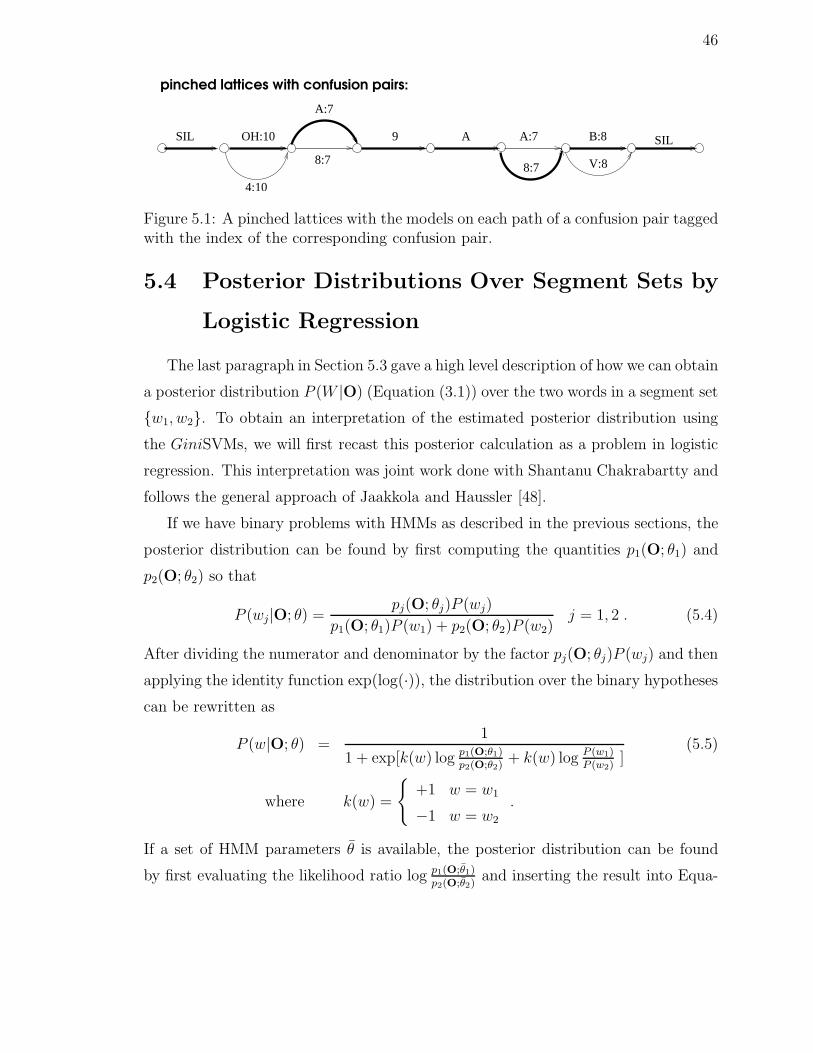
46

OH:10 ASIL SIL

pinched lattices with confusion pairs:

9

8:7

A:7

B:8

V:8

A:7

8:7

4:10

Figure 5.1: A pinched lattices with the models on each path of a confusion pair taggedwith the index of the corresponding confusion pair.

5.4 Posterior Distributions Over Segment Sets by

Logistic Regression

The last paragraph in Section 5.3 gave a high level description of how we can obtain

a posterior distribution P (W |O) (Equation (3.1)) over the two words in a segment set

w1, w2. To obtain an interpretation of the estimated posterior distribution using

the GiniSVMs, we will first recast this posterior calculation as a problem in logistic

regression. This interpretation was joint work done with Shantanu Chakrabartty and

follows the general approach of Jaakkola and Haussler [48].

If we have binary problems with HMMs as described in the previous sections, the

posterior distribution can be found by first computing the quantities p1(O; θ1) and

p2(O; θ2) so that

P (wj|O; θ) =pj(O; θj)P (wj)

p1(O; θ1)P (w1) + p2(O; θ2)P (w2)j = 1, 2 . (5.4)

After dividing the numerator and denominator by the factor pj(O; θj)P (wj) and then

applying the identity function exp(log(·)), the distribution over the binary hypotheses

can be rewritten as

P (w|O; θ) =1

1 + exp[k(w) log p1(O;θ1)p2(O;θ2)

+ k(w) log P (w1)P (w2)

](5.5)

where k(w) =

+1 w = w1

−1 w = w2

.

If a set of HMM parameters θ is available, the posterior distribution can be found

by first evaluating the likelihood ratio log p1(O;θ1)

p2(O;θ2)and inserting the result into Equa-

47

tion (5.5). If a new set of parameter values becomes available, the same approach

could be used to reestimate the posterior. Alternatively, the likelihood ratio could

be considered simply as a continuous function in θ whose value could be found by a

Taylor Series expansion around θ

logp1(O; θ1)

p2(O; θ2)= log

p1(O; θ1)

p2(O; θ2)+ (θ − θ) ∇θ log

p1(O; θ1)

p2(O; θ2)+ · · · (5.6)

which of course is only valid for θ ≈ θ.

If we ignore the higher order terms in this expansion, we can rewrite Equation 5.6

as

logp1(O; θ1)

p2(O; θ2)≈[

1 (θ − θ)]

log p1(O;θ1)

p2(O;θ2)

∇θ log p1(O;θ1)

p2(O;θ2)

. (5.7)

Note that the row vector on the R.H.S. are parameters that can be re-estimated

and the column vector on the R.H.S. is the log-likelihood ratio score-space, i.e., a

collection of statistics. If we augment these statistics as the following vector,

Ψ(O; θ) =

ln p1(O;θ1)p2(O;θ2)

∇θ1 ln p1(O; θ1)

−∇θ2 ln p2(O; θ2)

1

(5.8)

we can rewrite the posterior distribution (Equation 5.5) to obtain the following ap-

proximation at θ

P (w|O; θ) ≈1

1 + exp[ k(w) [1 (θ1 − θ1) (θ2 − θ2) log P (w1)P (w2)

] Ψ(O; θ) ]. (5.9)

We will realize this quantity by the logistic regression function

Pa(w|O; φ) =1

1 + exp[ k(w) φ⊤ Ψ(O; θ) ](5.10)

and Equation (5.9) is realized exactly if we set φ, the parameters to be estimated as,

φ =

φ0

φ1

φ2

φ3

=

1

θ1 − θ1

θ2 − θ2

log P (w1)P (w2)

. (5.11)

48

Our goal is to use estimation procedures developed for large margin classifiers

to estimate the parameters of Equation (5.10) and in this we will allow φ to vary

freely. This has various implications for our modeling assumptions. If we allow φ3

to vary, this is equivalent to computing Pa under a different prior distribution than

initially specified (However, in our experiments with GiniSVMs and score-spaces, we

always set φ3 as zero; this is reasonable since the log-likelihood ratio scores do not

provide any word information). If φ1 or φ2 vary, we allow the parameters of the

HMMs to vary from their nominal values θ1 and θ2. This might produce parameter

values that lead to invalid models, although we restrict ourselves here to the means

of the Gaussian observation distributions which can be varied freely. Variations in

φ0 are harder to interpret in terms of the original posterior distribution derived from

the HMMs; despite that, for the sake of improved performance we still allow this

parameter to vary (we will discuss the practical effect of φ0 in Chapter 6).

5.4.1 GiniSVMs as Parameter Estimators

Taking the form of Equation (5.10), we assume that we have a labeled training

set Oj , wjj and that we wish to refine the distribution Pa over the data according

to the following objective function

minφ

1

2‖φ‖2 − C

∑

j

log Pa(wj|Oj; φ) , (5.12)

where C is a trade-off parameter that determines how well Pa fits the training data.

The role of the regularization term ‖φ‖2 penalizes HMM parameter estimates that

vary too far from their initial values θ. Similarly, it allows reestimation of the prior

over the hypotheses, but prefers estimates that assign comparable likelihood to hy-

potheses.

If we define a binary valued indicator function over the training data

yj =

+1 wj = w1

−1 wj = w2

we can use the approximation techniques of S. Chakrabartty and G. Cauwenberghs[15]

49

to minimize Equation (5.12) where the dual is given by

1

2

∑

i,j

αi [ K( Ψ(Oi; θ), Ψ(Oj; θ) ) +2γ

Cδij ] αj − 2γ

∑

i

αi (5.13)

subject to∑

i

yiαi = 0, 0 ≤ αi ≤ C, (5.14)

where γ is the rate distortion factor chosen as 2 log 2 in the case of binary classes and

δij is the Kronecker delta function. The optimization can be carried out using the

GiniSVM Toolkit which is available online [13].

After the optimal parameters α are found, the posterior distribution of an obser-

vation is found as

Pa(w|O; φ) =1

1 + exp[ k(w) φ⊤ ζ( Ψ( O; θ ) ) ](5.15)

=1

1 + exp[ k(w)∑

i yi αi K( Ψ(Oi; θ), Ψ(O; θ) ) ]

, (5.16)

and φ can be written as φ =∑

i αi yi ζ( Ψ(Oi; θ) ), where ζ( · ) is the high-

dimensional space implied by the kernel K( · , · ) (see Section 4.1).

Using GiniSVM in this way allows us to estimate the posterior distribution under

penalized likelihood criterion of Equation (5.12). The distribution that results can be

used directly in the classification of new observations with the added benefit that the

form of the distribution in Equation (5.16) makes it easy to assign ‘confidence scores’

to hypotheses. This will be useful in the weighted hypothesis combination rescoring

procedures that will be described subsequently.

5.5 Modeling Issues

We will now discuss some of the modeling issues in training and decoding with

GiniSVMs in the code breaking framework.

5.5.1 Estimation of sufficient statistics

Calculating the features for training GiniSVMs, namely the scores, primarily re-

quires the estimation of the mixture-level posterior probabilities γi,s,j(t) in Equa-

50

tion (5.3). There are two algorithms one can use for computing them: the Viterbi

and the Baum-Welch algorithm.

We want to apply SVMS to word hypotheses in continuous speech recognition. In

these cases, the start and end times of the hypotheses are uncertain. One possibility

is to take the timing information from the first pass ASR output. Another alter-

native can be seen from the example in Figure 3.1, d. Consider the confusion pair

A:17 vs. J:17. We can compute the statistics by performing two Forward-Backward

calculations with respect to the transcriptions

SIL OH A:17 NINE A EIGHT B SILSIL OH J:17 NINE A EIGHT V SIL

where A:17 and J:17 are cloned versions of models A and J respectively. In this case,

since word boundaries are not fixed, duration is unknown and cannot be used for

normalization. The sum of the state occupancies as mentioned earlier can be used in

this case.

When we perform Forward-Backward calculations over the entire utterance, it is

possible to also consider the alternatives paths in the neighboring confusion segments.

For the confusion pair B:5 vs. V:5 in Figure 3.1, d, this would imply considering the

following four hypotheses:

SIL OH A NINE A EIGHT B:5 SILSIL OH A NINE A EIGHT V:5 SILSIL OH A NINE A A B:5 SILSIL OH A NINE A A V:5 SIL

5.5.2 Normalization

Scores have to be normalized for the sequence length T , as they are accumulators

over the individual observations o. If time segmentations of the utterance at the

word level are available, we can simply normalize the scores with the length of the

word. Otherwise, it is more appropriate to scale each mixture posterior estimate by

the sum of the state occupancy over the entire utterance is more appropriate [90],

i.e.,∑T

t=1 γs(t), where s is the state index and γs(t) is as defined in Section 2.3.

While a linear classifier can subsume a bias in the training, the parameter search (αi

in Equation 5.13) can be made more effective by ensuring that the training data is

51

normalized. We first adjust the scores for each acoustic segment via mean and vari-

ance normalization. The normalized scores are given by

ϕN(O) = Σ−1/2sc [ϕ(O) − µsc], (5.17)

where µsc and Σsc are estimates of the mean and variances of the scores as computed

over the training data of the SVM. Ideally, the SVM training will subsume the µsc

bias and the variance normalization would be performed by the scaling matrix Σsc as

ϕN(O) = Σ−1/2sc ϕ(O) (5.18)

where Σsc =∫

ϕ(O)′ϕ(O)P (O|θ)dO. For implementation purposes, the scaling ma-

trix is approximated over the training data as

Σsc =1

N − 1

∑

(ϕ(O) − µsc)⊤(ϕ(O) − µsc) (5.19)

where µsc = 1N

∑

ϕ(O), and N is the number of training samples for the SVM.

However we used a diagonal approximation for Σsc since the inversion of the full

matrix Σsc is problematic.

5.5.3 Dimensionality Reduction

For efficiency and modeling robustness there may be value in reducing the di-

mensionality of the score-space. There has been research [5, 90] to estimate the

information content of each dimension so that non-informative dimensions can be

discarded. Assuming independence between dimensions, the goodness of a dimension

can be found based on Fisher discriminant scores as [90]

g[d] =|µsc[1][d] − µsc[2][d]|

Σsc[1][d] + Σsc[2][d](5.20)

where µsc[i](d) is the dth dimension of the mean of the scores of the training data

with label i and Σsc[i][d] are the corresponding diagonal variances. SVMs can then be

trained only in the most informative dimensions by applying a pruning threshold to

g[d].

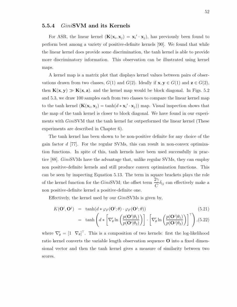
52

5.5.4 GiniSVM and its Kernels

For ASR, the linear kernel (K(xi,xj) = xi′ · xj), has previously been found to

perform best among a variety of positive-definite kernels [90]. We found that while

the linear kernel does provide some discrimination, the tanh kernel is able to provide

more discriminatory information. This observation can be illustrated using kernel

maps.

A kernel map is a matrix plot that displays kernel values between pairs of obser-

vations drawn from two classes, G(1) and G(2). Ideally if x,y ∈ G(1) and z ∈ G(2),

then K(x,y) ≫ K(x, z). and the kernel map would be block diagonal. In Figs. 5.2

and 5.3, we draw 100 samples each from two classes to compare the linear kernel map

to the tanh kernel (K(xi,xj) = tanh(d ∗ xi′ · xj)) map. Visual inspection shows that

the map of the tanh kernel is closer to block diagonal. We have found in our experi-

ments with GiniSVM that the tanh kernel far outperformed the linear kernel (These

experiments are described in Chapter 6).

The tanh kernel has been shown to be non-positive definite for any choice of the

gain factor d [77]. For the regular SVMs, this can result in non-convex optimiza-

tion functions. In spite of this, tanh kernels have been used successfully in prac-

tice [88]. GiniSVMs have the advantage that, unlike regular SVMs, they can employ

non positive-definite kernels and still produce convex optimization functions. This

can be seen by inspecting Equation 5.13. The term in square brackets plays the role

of the kernel function for the GiniSVM; the offset term2γ

Cδij can effectively make a

non positive-definite kernel a positive-definite one.

Effectively, the kernel used by our GiniSVMs is given by,

K(Oi,Oj) = tanh(d ∗ ϕF (Oi; θ) · ϕF (Oj; θ)) (5.21)

= tanh

(

d ∗

[

∇′θ ln

(

p(Oi|θ1)

p(Oi|θ2)

)]

·

[

∇′θ ln

(

p(Oj |θ1)

p(Oj |θ2)

)]⊤)

,(5.22)

where ∇′θ = [1 ∇θ]

⊤. This is a composition of two kernels: first the log-likelihood

ratio kernel converts the variable length observation sequence O into a fixed dimen-

sional vector and then the tanh kernel gives a measure of similarity between two

scores.

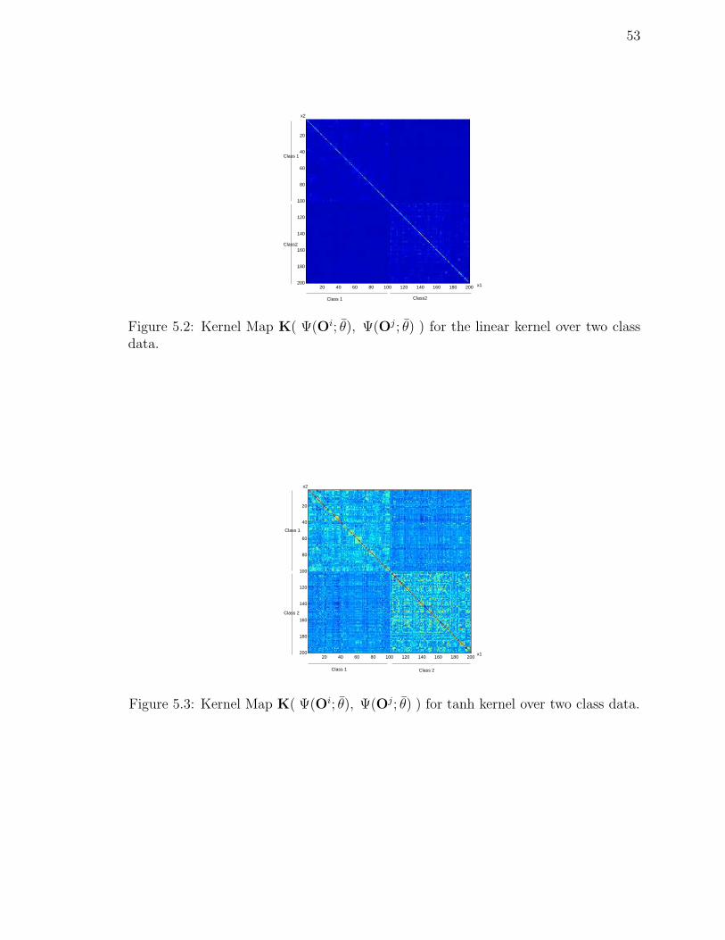
53

20 40 60 80 100 120 140 160 180 200

20

40

60

80

100

120

140

160

180

200

Class 1

Class 1

Class2

Class2

x2

x1

Figure 5.2: Kernel Map K( Ψ(Oi; θ), Ψ(Oj ; θ) ) for the linear kernel over two classdata.

20 40 60 80 100 120 140 160 180 200

20

40

60

80

100

120

140

160

180

200

Class 1

Class 1

Class 2

Class 2

x2

x1

Figure 5.3: Kernel Map K( Ψ(Oi; θ), Ψ(Oj; θ) ) for tanh kernel over two class data.

54

5.6 The SVM-Code Breaking framework

We now describe the steps we performed to incorporate SVMs in the code breaking

framework.

1. Identifying confusion sets in the test set. Initial test set lattices are generated us-

ing the baseline HMM system to decode the speech in the test set. The lattices

produced are then aligned against the reference transcriptions [42]. Period-1

lattice cutting is performed and each sub-lattice is pruned (by the word poste-

rior) to contain two competing words (the methods of pruning were elaborated

in Section 3.2). This process identifies regions of confusion in the test set.

The most frequently occurring confusion pairs (confusable words) are kept, and

their associated acoustic segments are identified, retaining time boundaries (if

required for the estimation of sufficient statistics) and the true identity of the

word spoken.

2. Identifying appropriate training data. To obtain training data, we either repeat

the process of identification of confusions over the training set with the differ-

ence that the path for alignment is the transcription of the utterance or we

simply create training data for each confusion pair between w1 and w2 as every

instance of the individual words. These methods are elaborated and contrasted

in Section 3.4.

3. Training SVMs for each confusion pair. For each acoustic segment in every sub-

lattice of the training set, likelihood-ratio scores as given by Equation (5.2) are

generated. The dimension of these scores is equal to the sum of the number of

parameters of the two competing HMMs plus one. If necessary, the dimension

of the score-space is reduced using the goodness criterion (Equation (5.20))

with appropriate thresholds. SVMs for each confusion pair are then trained in

our normalized score-space using the appropriate acoustic segments identified

as above.

55

4. Decoding with SVMs. We then generate appropriate likelihood-ratio scores for

each segment in the test set associated with each confusion pair in the lattice.

The corresponding SVM is applied to each acoustic segment. If we simply use

the SVMs to make hard decisions, we can then concatenate the outputs of the

SVMs in the regions of low confidence with the HMM outputs in the regions

of high confidence. This can then be taken as the final hypothesis of the code-

breaking system.

5. Posterior-based System Combination. We can also apply the SVM to each

acoustic segment to obtain posterior probability estimates over the hypotheses

in the segment. We now have the HMM and the SVM-code breaking system

hypotheses along with their posterior estimates. If these posterior estimates

serve as reliable confidence measures, we can combine the system hypotheses to

yield better performance. Several voting schemes have been proposed on how

to choose between the outputs of two or more systems. We use either

p+(i) =ph(i) + ps(i)

2. (5.23)

or

p×(i) =ph(i)ps(i)

ph(1)ps(1) + ph(2)ps(2). (5.24)

where ph(1) and ph(2) are the posterior estimates of the two competing words

in a segment as estimated by the HMM system and ps(1) and ps(2) of the

SVM-code-breaking system. Both these schemes then pick the word with the

new higher estimate. We can then concatenate the outputs from the individual

segments with the HMM outputs in the regions of high confidence to obtain our

final hypothesis.

5.7 Summary

This chapter discussed the framework for using Support Vector Machines (SVMs)

in the code-breaking framework. For each of the segment sets of a confusion pair,

we use the Hidden Markov Models (HMMs) representing the two words to generate

56

fixed dimensional features for the SVMs; we use the GiniSVMs to estimate posterior

probabilities over the hypotheses for each segment set; and we finally use the posterior

probability estimates to combine the outputs of the original HMMs and the SVMs.

In the next chapter, we will validate this new framework on a speech recognition task.

5.8 Previous Work

There have been some research efforts which can be interpreted as code-breaking.

We will review them first and point out the differences compared to our approach.

SVMs have also been used previously in other speech tasks; we will briefly review

these approaches.

5.8.1 Approaches Related to Code Breaking

Code-breaking for speech recognition was first proposed by F. Jelinek [52] as a

technique to enhance an HMM speech recognizer. The idea was to build a special-

ized language (or acoustic) model for the word sequences (or state sequences) that

appear in each lattice. We have extended this idea by introducing the concept of low-

confidence regions and of training specialized decoders only for specific confusions of

the original decoder.

M. J. F. Gales and M. Layton [38] extend the framework introduced by Smith et

al [91] to large vocabulary continuous speech recognition using the ideas presented

by V. Venkataramani et al [95]. Lattices are converted into a sequence of confusion

networks, similar in structure to confusion pairs. Their training of the HMMs to

generate scores is interesting: the HMM parameter estimation procedure is coupled

with that of the SVM’s. This leads to scores that are more discriminative in nature.

They report a decrease in errors counts over a RT04 development set [29] but no

improvements in error rates. While their framework is very similar to ours, when we

apply code-breaking to large vocabulary recognition, we will choose the instances of

confusion pairs we want to process based on a threshold that results in high quality

segment sets; this filtering of the segment sets will be elaborated in Chapter 7.

57

AdaBoost [36] is a learning algorithm that first identifies training data that are

erroneously classified. Several instances of the original classifier are trained over dif-

ferent distributions of the training data with an emphasis on the erroneously classified

data. The individual classifiers then vote to produce the final output. Note that this

identification is done over the training data and not over the test data. We attempt to

identify possible errors of the original classifier over the test data in an unsupervised

fashion. We then build decoders for each specific confusion pair.

S. Fine et al. [33] propose a technique that is close to code-breaking. A Confusion

Set (CS) is created by comparing GMM likelihoods of alternate phone hypotheses

to the baseline. SVMs then process the HMM feature vectors to choose the output

phone. They note that improvements can only be obtained if the SVMs perform better

than the GMMs on the CS. S. Fine et al. [33] attempt to exploit the fact that GMM

and SVM classifiers, with roughly the same level of performance exhibit uncorrelated

errors, can be combined to produce a better classifier. An all-pair Error-Correcting

Output Code technique was used to map the binary classifiers into a multi-class

framework. They note substantial improvements on a connected digit recognition

task at matched or slightly noisy conditions. While our motivation is similar in

that we only want to apply SVMs in low confidence regions, we derive our word

based confidence sets from lattice posteriors and alignments. The use of score-spaces

derived from word based models gives us word hypotheses directly.

J. Fritsch and M. Finke [37] uses a hierarchical clustering approach to break down

the task of discriminating between thousands of classes (HMM states) into a smaller

classification tasks; their motivation is the application of connectionist methods [7]

for large vocabulary recognition. The smaller tasks are determined ahead of recogni-

tion by agglomerative clustering on information divergence. During recognition, the

posterior probability of a class (HMM state) is obtained by traversing the hierarchy

and reaching a leaf. While we also propose a divide-and-conquer approach, we are

motivated to identify regions of weakness of a GMM-based HMM based recognizer

and during the process of recognition; we then produce a second-pass hypothesis in

these regions. We are explicitly attempting to enhance an existing system rather than

modify it.

58

5.8.2 Applications of SVMs in Speech

In this subsection, we will first describe earlier work involving the use of SVMs in

speech recognition and then distinguish them from our approach. We will also look at

the extensions to Fisher scores beyond log-likelihood ratio scores. For thoroughness,

we finally briefly discuss the use of SVMs in other speech based tasks like speaker

identification, utterance classification, web audio classification, etc.

S. E. Golowich and D. X. Sun [44] used SVMs in a hybrid approach to model

the emission densities in a HMM based phone recognizer. SVMs were viewed as

an approximation to smoothing spline logistic regression [97] to directly generate

normalized scores. The connectionist acoustic modeling approach [7] was followed to

obtain generative probabilities for each frame. Polynomial kernels were used. It was

found that the error structure of the outputs obtained from the SVM/HMM based and

the Gaussian-HMM based system was substantially different and thus improvements

could be obtained upon system combination on a TIMIT corpus. While ours is also

a hybrid approach we apply our SVMs in low-confidence regions alone as a rescoring

approach; we still use GMMs as emission densities in our first pass HMM system. We

also derive our SVM features from the HMMs and not the HMM input features.

A. Ganapathiraju et al. [40] developed an HMM/SVM hybrid system in an N-

best list rescoring framework. The N-best lists and acoustic segmentations for each

hypothesis were obtained from baseline HMM models. Each phone segment in an hy-

pothesis was broken into three regions in the ratio 3-4-3. The acoustic observations

belonging to each of these regions were averaged resulting in a fixed dimensional vec-

tor. RBF kernels and polynomial kernels were used. One-vs-all flavor SVMs were then

applied to estimate posterior probabilities which were used for system combination

with the original HMM system and for rescoring the N-best list. Significant improve-

ments were reported on a Switchboard task; this was the first instance of use of SVMs

in a complex large-vocabulary task. While we also use a rescoring framework, the

rescoring is done selectively on regions of low-confidence identified in lattices; we do

not apply SVMs for every segment. Also, our SVMs features are derived from HMMs

themselves and not from the input features.

59

P. Clarkson and P. Moreno [17] used the same 3-4-3 idea as [40] and studied the

performance of SVMs in vowel and phone classification. They also give a detailed

analysis of challenges involved in applying SVMs for speech recognition.

N. Smith et al. [91, 90] introduced and developed several techniques (log-likelihood

ratio score-spaces, score-space normalization, selection of dimensions in score-spaces)

that are used in this thesis. They were the first to apply Fisher Kernels to speech

recognition. They evaluated their techniques on an isolated letter database and

showed that a hard-decision SVM system outperforms a state-of-the-art MMI trained

HMM-based system. They used RBF, linear, and polynomial kernels. With our code-

breaking framework we have extended the use of score-spaces and SVMs to continuous

speech recognition. Moreover with GiniSVMs we are able to estimate posterior prob-

abilities to study system combination schemes and also use tanh kernels.

J. Salomon et al. [85] use a frame-by-frame classification approach to estimate a

phone conditional probability density function. By decoding this pdf sequence into

a word string they avoid the problem of dealing with variable-length feature vectors.

They notice the problem of scaling in SVMs when given massive amounts of training

data and use of the Kernel Fisher Discriminant [65] to alleviate the problem.

I. Bazzi and D. Katabi [4] create a fixed length observation by selecting a fixed

number of the most dissimilar feature vectors. They used Principal Component Anal-

ysis to reduce the dimensions and then used to train SVMs. They compared 1-vs.rest

classifiers and 1-vs-1 classifiers on a digit recognition task. They report the 1-v-rest

flavor performed better. We consider a continuous speech recognition task and use

SVMs in a smart rescoring framework.

A. Juneja and C. Espy-Wilson [54] use SVMs for binary phonetic feature classifi-

cation to represent speech as bundles of binary valued articulatory phonetic features

or landmarks. Pronunciation models based on phonetic features are used to constrain

the landmark sequences and to narrow the classification of place and voicing. They

show that their Event-Based system performs favorably to HMM based system on a

TIMIT database. We do not propose a change in the front end or to supplant HMMs.

We use SVMs only in low-confidence regions of the HMMs.

The Landmark team [46] of the 2004 Johns Hopkins Summer Workshop studied

60

the integration of landmarks (detected using SVMs in the same way as A. Juneja

and C. Espy-Wilson [54]) in speech recognition systems as features for pronunciation

models that are based on either SVMs, dynamic Bayesian networks, or maximum

entropy classification. These pronunciation models were then used to rescore word

level lattices on the 2003 NIST rich text transcription task. The word lattices were

restricted to confusion networks using local information [100]. They report WER

reductions on training data and on a subset of the development test data, but no

statistically significant WER reductions the complete test set. While we also propose

using SVMs only in low-confidence regions, these regions are found using utterance

level information that does not disrupt the original structure of the lattice. The

features for our SVMs are also obtained from well-trained HMMs.

Forward Decoding Kernel Machines (FDKM) [15] perform maximum a poste-

riori forward sequence decoding. The transition probabilities are regressed by the

GiniSVM, which was reviewed here. A kernel expansion of acoustic features is ob-

tained; training is performed by maximizing a lower bound on a regularized form of

cross-entropy. FDKM techniques were mainly developed to implement speech algo-

rithms in low power VLSI technology.

There has also been considerable use of SVMs in speaker verification also. Fine et

al. [32, 31] used Fisher Kernels to obtain features for the SVMs. They exploited the

fact that when GMM and SVM classifiers with roughly the same level of performance

exhibit uncorrelated errors they can be combined to produce a better classifier.

N. Oliver et al [76] study extend the Fisher kernels to Natural kernels and study

its properties. W. M. Campell [10] developed an alternate kernel for speaker recog-

nition, the Generalized Linear Discriminant Sequence (KDLS) kernel. The KLDS

kernel combines a speaker model with a generalized linear approximation and allows

processing of utterances as entire sequences.

V. Wan and S. Renalis [98] have studied the use of the log-likelihood ratio score-

space for speaker verification tasks and report improvements over the Fisher Kernel.

They also use a different method of normalization called spherical normalization,

to reduce variations in magnitude of the dot products. Later, V. Wan and S. Re-

nals [99] compared the performance of a variety of kernels when using support vector

61

machines on speaker verification and speaker identification tasks. They found the

likelihood ratio kernel to be the best performing kernel among a variety of kernels.

W. M. Campbell et al. [11] performed speaker verification using idiolectal information,

i.e., a vector of unigram and bigram stats, as the feature space for training SVMs.

Y. Liu et al. [103] account for different costs in misclassification when training SVMs.

P. Moreno and R. Rifkin [69] have also used Fisher Scores for web audio classifi-

cation. P. J. Moreno and P. Ho [67] later used SVMs with Fisher Scores for speaker

verification. They developed a Kullback-Leibler Divergence Based Kernel and showed

superior performance when compared to Fisher Kernels. Instead of assuming a gener-

ative model for the data, they represent each observation sequence by its unique PDF;

the similarity measure between two observation sequences is taken to be the diver-

gence of the PDFs estimated for two sequences. They report extremely good results

even with a simple single full covariance Gaussian models. Moreno et al. have also

applied these Kullback-Leibler Divergence Based Kernels also to image classification

tasks [68].

SVMs have also been used for other speech tasks also. C. Cortes et al. [18]

developed rational kernels that use the word (or phone) strings in two lattices to

determine if the lattices are similar. This lattice based kernel was used in a spoken-

dialog system to classify an utterance as one of a finite number of classes. SVMs

have also been used to guess the emotion of the speaker using features derived from

the signal, pitch, energy, and spectral contours [89]. C. Ma and M. A. Rudolph [62]

used SVMs for utterance verification. Kernel ideas have also been used in eigen voice

adaptation [63]. M. Davy and S. Godsill [20] use SVMs as a novelty detector for

audio signal representation. B. Krishnapuram and L. Carin [56] use Fisher Scores for

multiaspect target recognition. SVMs have also been used to detect stop consonants

in continuous speech [71]. SVMs have been used to classify speech as either adult

or child voiced [70] based on acoustic and linguistic scores. N. Mesgarani et al. [64]

use SVMs to discriminate speech from non-speech sounds using SVMs trained on

auditory features.

62

Chapter 6

Validating Code Breaking

We have now introduced and described all the various stages and some of the mod-

eling issues involved in the code-breaking framework. Chapter 3 described the lattice

cutting algorithm and the appropriate pruning procedures to obtain binary confusion

sets. Chapter 4 reviewed the GiniSupport Vector Machines (GiniSVMs) and how

we obtain posterior probability estimates from them. Chapter 5 discussed how to

use GiniSVMs in speech recognition and in code-breaking in particular, to estimate

posterior probabilities over the hypotheses in the segment sets; it also discussed the

system combination schemes between the original HMM and the SVM code-breaking

systems to obtain our final system output.

This chapter will put the code-breaking framework into practice and present ex-

periments validating the approach. We will first describe the corpus we studied before

describing the baseline Hidden Markov Model (HMM) systems. We then present the

Support Vector Machines (SVM) code-breaking systems and discuss their perfor-

mance and also the improvements we obtain from system combination schemes. We

then discuss some alternate baseline systems that arise due to the refinement of the

training data. We conclude with a discussion of using constrained estimation methods

to apply code-breaking to Large Vocabulary tasks.

63

6.1 The OGI-Alphadigits corpus

The specific corpus we use is the OGI-Alphadigits corpus [72]. This is a small

vocabulary task that is fairly challenging. The baseline Word Error Rates (WERs)

for HMM systems trained under the Maximum-Likelihood (ML) criterion are around

10%; this ensures that there are enough number of errors to support analysis. The

corpus has a vocabulary of 36 words: 26 letters and 10 digits. The corpus has 46,730

training and 3,112 test utterances. There is no restriction on the sequence of the

words allowed; each utterance is a random six word string.

There are several reasons to work on such a corpus. When the size of the vocab-

ulary increases, the complexity of state-of-the-art speech recognizers also increases.

We chose a small vocabulary task so that we can present our ideas without having to

account for such complications.

A large vocabulary would also introduce issues of sparsity (discussed in detail in

later chapters); i.e., the most frequently occurring confusions will not occur enough

number of times for us to obtain substantial improvements. While we are ultimately

interested in obtaining substantial improvements, sparsity is not directly related to

the feasibility of the code-breaking framework; it only fixes an upper bound on the

improvements that we can expect from the framework. We are now interested in find-

ing out if the second-pass decoders (namely, GiniSVMs) can show any improvements

in the low-confidence regions of HMM decoders.

Our main goal right now is to validate the idea of acoustic code-breaking; i.e.,

code-breaking where the specialized decoders are trained on acoustic information

only (specifically, GiniSVMs trained on score-spaces). A corpus with language model

information would imply that there is extra information besides the acoustics which

cannot be captured by the score-spaces we described. So, we want a corpus where all

discriminative information is available in the acoustics alone.

In spite of these restrictions, such a task is not unrelated to real-world systems.

There are various applications like package tracking systems or flight information

systems where the user is asked to say a string of letters and digits.

64

6.2 Baseline Systems

6.2.1 ML and MMI models

We will now describe the training procedure for the various baseline models. The

data are parametrized as 13 dimensional Mel-Frequency Cepstral Coefficient (MFCC)

vectors with first and second order differentials. The baseline ML models were trained

following the standard HTK procedure [27]. Word based HMMs were trained for each

of the 36 words. The word models were left-to-right with approximately 20 states

each, and had 12 mixtures per speech state.

The number of states for each word was chosen to be one-half of the mean duration

of the word [55]. The word durations are determined by first training a system with

each word model having 10 states. Then a forced alignment of the models to the

training data is generated and the word duration statistics are computed from this

forced word alignment. The baseline system has a total of 825 states.

The AT&T decoder [66] was used to generate lattices on both the training and the

test set. Since each utterance is a random six word string, an unweighted free loop

grammar was used during decoding. The ML baseline WER is 10.70%; the Lattice

Oracle Error Rate for the ML lattices is 2.00%. MMI training [74, 102] was then

performed at the word level using word time boundaries taken from the lattices. A

new set of lattices for both the training and the test sets was then generated using

the MMI models. The MMI WER was 9.07% and the Lattice Oracle Error Rate for

these lattices was 1.70%. A more detailed description of the MMI training can be

found in the paper by V. Doumpiotis et al. [23]. The WERs of these HMM systems

are listed in the WER column of Table 6.1.

6.2.2 Lattice Pinching

We then performed period-1 lattice cutting on both the training and test MMI

lattices as we described in Section 3.1. We discard the NULL hypothesis and alter-

natives more than a word long in each segment. The number of confusable words in

each segment was restricted to two by keeping behind the two most probable words

65

HMM Training Word LatticeCriterion Error Rate Error Rate

ML 10.73 2.00MMI 9.07 1.70

PLMMI 7.98 1.80

Table 6.1: Performance of various baseline HMM systems. ML: Baseline HMMstrained under the ML criterion; MMI: The ML HMMs are trained using MMI;PLMMI: The MMI HMMs were MMI trained on the MMI pinched lattices. Therestriction in the last column is that the confusion pairs allowed are only the 50 mostfrequently observed ones in the MMI case.

in each segment. We will study the effects of restricting the lattices hypothesis on

LER in the next section. At this point there are two sets of confusion pairs from the

pinched lattices: one set comes from the training data, and the other from the test

data. Examples of the frequent confusion pairs are (F,S), (B,V) and (TWO,U).

Rationale. The most ambitious formulation of acoustic code-breaking is to first

identify all acoustic confusions in the test set, and then return to the training set to

find any data that can be used to train models to remove the confusion. To present

these techniques and show that they can be effective, we have chosen for simplicity,

to focus on modeling the most frequent errors found in training.

Earlier work [22] has verified that training set errors found in this way are good

predictors of errors that will be encountered in unseen data. Table 6.2 compares the

count of the number of instances of frequently occurring confusion pairs found on the

training set to that found on the test set. The index listed in the first column gives

the rank of the confusion pair as determined by the number of errors found on the

test set. A segment set is counted as an error if the MAP hypothesis in the set is

not the truth. More errors involving the confusion pair F S was identified than those

involving V Z; Table 6.2 appropriately lists F S a higher rank (rank 1) than V Z(rank

2). There is good agreement among the top eight sets identified in each case, after

which there is some divergence. Thus we are justified in focusing on modeling the

most frequent errors found in training.

We keep the 50 confusion pairs that are observed most frequently in the training

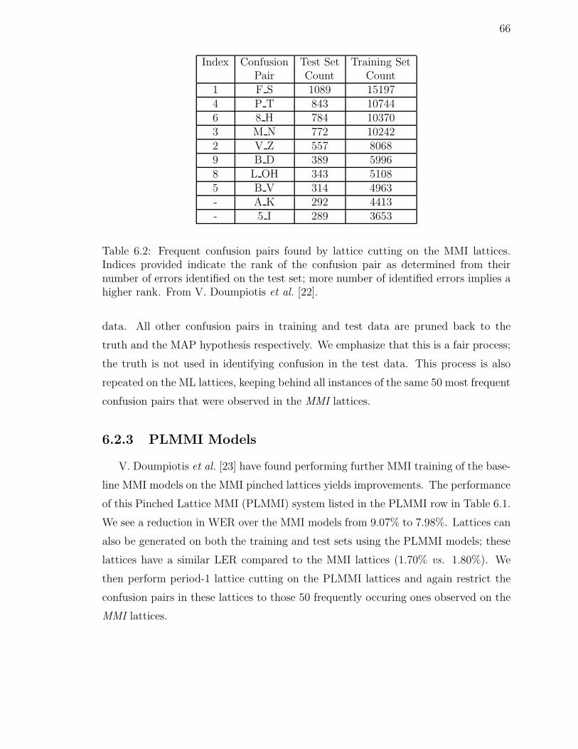
66

Index Confusion Test Set Training SetPair Count Count

1 F S 1089 151974 P T 843 107446 8 H 784 103703 M N 772 102422 V Z 557 80689 B D 389 59968 L OH 343 51085 B V 314 4963- A K 292 4413- 5 I 289 3653

Table 6.2: Frequent confusion pairs found by lattice cutting on the MMI lattices.Indices provided indicate the rank of the confusion pair as determined from theirnumber of errors identified on the test set; more number of identified errors implies ahigher rank. From V. Doumpiotis et al. [22].

data. All other confusion pairs in training and test data are pruned back to the

truth and the MAP hypothesis respectively. We emphasize that this is a fair process;

the truth is not used in identifying confusion in the test data. This process is also

repeated on the ML lattices, keeping behind all instances of the same 50 most frequent

confusion pairs that were observed in the MMI lattices.

6.2.3 PLMMI Models

V. Doumpiotis et al. [23] have found performing further MMI training of the base-

line MMI models on the MMI pinched lattices yields improvements. The performance

of this Pinched Lattice MMI (PLMMI) system listed in the PLMMI row in Table 6.1.

We see a reduction in WER over the MMI models from 9.07% to 7.98%. Lattices can

also be generated on both the training and test sets using the PLMMI models; these

lattices have a similar LER compared to the MMI lattices (1.70% vs. 1.80%). We

then perform period-1 lattice cutting on the PLMMI lattices and again restrict the

confusion pairs in these lattices to those 50 frequently occuring ones observed on the

MMI lattices.

67

HMM Training WER LER 50 frequent binary Binary confusionsCriterion confusions LER LER

ML 10.73 2.00 5.60 4.87MMI 9.07 1.70 4.65 4.07

PLMMI 7.98 1.80 4.68 3.93

Table 6.3: Measuring the approximations induced by restricting pinched test setlattices to binary confusion problems. ‘50 frequent binary confusions LER’ refersto to LER after restricting the pinched lattice to the 50 most frequently occurringconfusion found on the MMI training set lattices. ‘Binary confusions LER’ is theLER after restricting the pinched lattice to all identified binary confusions.

6.2.4 Quantifying the Search Space Approximations

To quantify the approximations in the search spaces induced by focusing on the

50 most frequent confusion pairs alone, we measured the LERs of the corresponding

lattices. These LERs for the various lattices are listed in Table 6.3.

For the ML lattices, this approximation increased the Lattice Oracle Error Rate

from 2.00% to 5.60% and for the MMI lattices from 1.70% to 4.11%. Note that

while the LERs of the original lattices generated from the ML and the MMI models

are comparable (2.00% vs. 1.70%), the restricted LER for the MMI models are

significantly better (5.60% vs. 4.65%). This is in spite of the number of identified

confusions in the test set being the same for both the models (≈8400 instances). This

illustrates the discriminative power of the MMI models; the correct hypothesis was

perceived more probable by the MMI models more often than by the ML models and

thus created more instances of confusions with the truth as one of the hypotheses.

However, note that while the performance of the PLMMI models are significantly

better than that of the MI models (9.07% vs. 7.98%) the LER of the PLMMI lattices

and their restricted versions are are not better than their MMI counterparts (4.65% vs.

4.68%). While the PLMMI models allow fewer instances of confusion pairs compared

to the MMI models (there were ≈8400 instances for the MMI case and ≈5400 instances

for the PLMMI case), we would still expect the PLMMI models to find a better search

space than the MMI models.

The reason for this seemingly inconsistent result becomes clear when we look

68

at the last column ‘Binary confusions LER’ of Table 6.3. When we consider all

possible binary confusions, the PLMMI lattices do give a better search space than

the MMI lattices (4.07% vs. 3.93%). This points to the mismatch in the frequent

confusions observed by the PLMMI models to those observed by the MMI models.

The weaknesses of the MMI models are no longer the weaknesses of the PLMMI

models.

Finally, note that for all the models, restricting the generated lattices to the 50

most frequent binary confusions still offers scope to obtain substantial improvements

over the corresponding baselines. Specifically, if we solve all binary confusions identi-

fied in the MMI lattices correctly, we would have obtained a (9.07-4.65)/9.07=48.7%

relative improvement.

6.3 SVM code-breaking systems

GiniSVMs were trained for the 50 dominant confusion pairs using the GiniSVM

Toolkit [13] based on the lattices generated by the ML system. The word time

boundaries of the training samples were extracted from the lattices by performing two

forced alignments (as described in Section 5.5.1). The statistics needed for the SVM

computation were found using the Forward-Backward procedure over these segments;

in particular the mixture posteriors of the HMM observation distributions were found

in this way. Log-likelihood ratio scores were generated from the 12 mixture MMI

models and normalized by the segment length as described in Section 5.5.1.

We initially investigated score spaces constructed from both Gaussian mean and

variance parameters. However training SVMs in this complete score space is imprac-

tical since the dimension of the score space is prohibitively large; the complete dimen-

sion is approximately 40,000. Filtering these dimensions based on Equation( 5.20)

made training feasible, however performance was not encouraging. We hypothesize

that there is significant dependence between the model means and variances so that

the underlying assumptions of the goodness criterion are violated.

We then used only the filtered mean sub-space scores for training SVMs (training

on the unfiltered mean sub-space is still impractical because of the prohibitively high

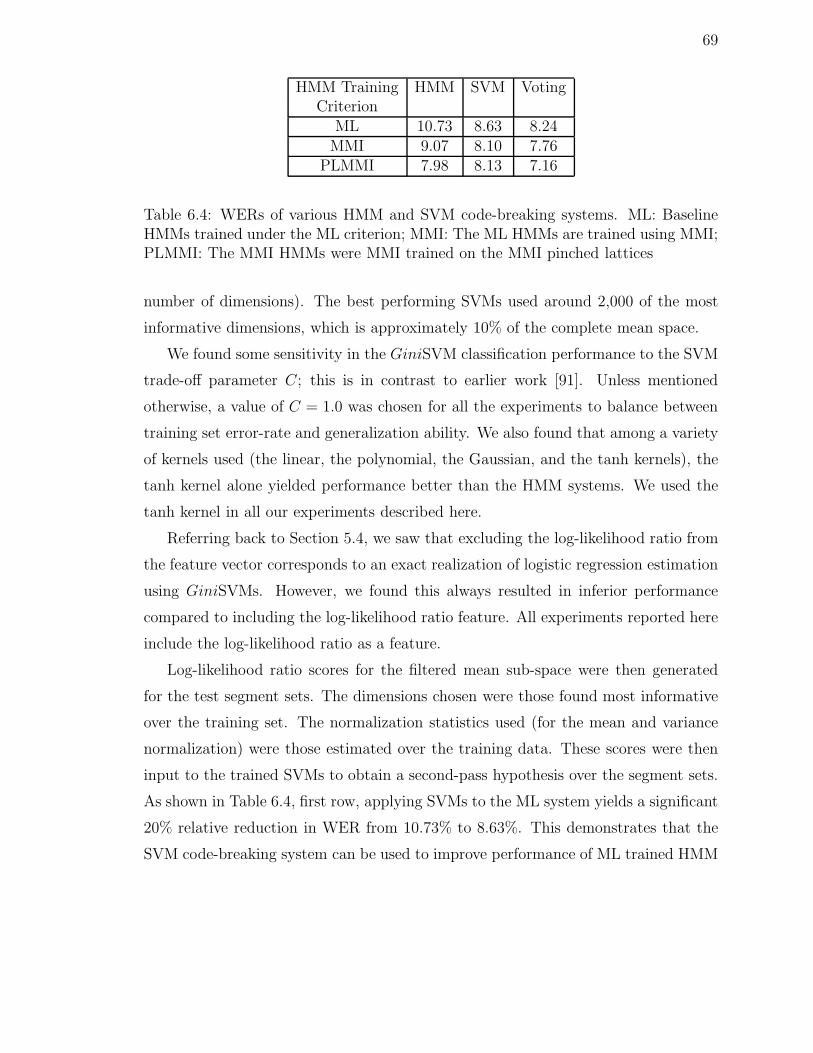
69

HMM Training HMM SVM VotingCriterion

ML 10.73 8.63 8.24MMI 9.07 8.10 7.76

PLMMI 7.98 8.13 7.16

Table 6.4: WERs of various HMM and SVM code-breaking systems. ML: BaselineHMMs trained under the ML criterion; MMI: The ML HMMs are trained using MMI;PLMMI: The MMI HMMs were MMI trained on the MMI pinched lattices

number of dimensions). The best performing SVMs used around 2,000 of the most

informative dimensions, which is approximately 10% of the complete mean space.

We found some sensitivity in the GiniSVM classification performance to the SVM

trade-off parameter C; this is in contrast to earlier work [91]. Unless mentioned

otherwise, a value of C = 1.0 was chosen for all the experiments to balance between

training set error-rate and generalization ability. We also found that among a variety

of kernels used (the linear, the polynomial, the Gaussian, and the tanh kernels), the

tanh kernel alone yielded performance better than the HMM systems. We used the

tanh kernel in all our experiments described here.

Referring back to Section 5.4, we saw that excluding the log-likelihood ratio from

the feature vector corresponds to an exact realization of logistic regression estimation

using GiniSVMs. However, we found this always resulted in inferior performance

compared to including the log-likelihood ratio feature. All experiments reported here

include the log-likelihood ratio as a feature.

Log-likelihood ratio scores for the filtered mean sub-space were then generated

for the test segment sets. The dimensions chosen were those found most informative

over the training set. The normalization statistics used (for the mean and variance

normalization) were those estimated over the training data. These scores were then

input to the trained SVMs to obtain a second-pass hypothesis over the segment sets.

As shown in Table 6.4, first row, applying SVMs to the ML system yields a significant

20% relative reduction in WER from 10.73% to 8.63%. This demonstrates that the

SVM code-breaking system can be used to improve performance of ML trained HMM

70

continuous speech recognition systems.

This process was then repeated for the case of the MMI models; the word time

boundaries were obtained from the MMI lattices. From the second row in Table 6.4,

we see that the SVM system gives a significant 10% relative decrease in WER from

9.07% to 8.10%. This demonstrates that the SVM code-breaking system can be also

used to improve performance of discriminatively trained HMM continuous speech

recognition systems. Finally we can see that MMI-SVM performs comparably to

PLMMI HMM systems also (8.10% vs. 7.98%).

6.3.1 Voting

We observed the MMI and the SVM code-breaking system hypotheses greatly

differed from each other i.e., if we took the MMI hypotheses as the truth and scored

the SVM code-breaking system hypotheses against it, we find a WER of around

4%. Such situations where the HMM and SVM hypotheses have uncorrelated error

patterns have been observed in some but not all previous work [32, 44, 91]. This

suggests that hypothesis selection can produce an output better than either of the

individual outputs. Ideally the voting schemes will be based on posterior estimates

provided by each system. Transforming HMM acoustic likelihoods into posteriors is

well established [101]. However we need to validate the posterior estimates of the

GiniSVM hypothesis as confidence scores. The quality of a confidence score can be

measured by the Normalized Cross-Entropy (NCE) as used by [30].

NCE =

Hmax +∑

correct w

log2(p(w)) +∑

incorrect w

log2(1 − p(w))

Hmax(6.1)

where Hmax = −n log2(pc) − (N − n) log2(1 − pc)

n = # of correctly hypothesized words

N = # of hypothesized words

pc = average probability that an output word is correct(n

N)

p(w) = the confidence measure as a function of the output word w.

NCE is such that the higher the score the better the relative reliability of a system’s

71

confidence estimates. The NCE estimates for the GiniSVM output were encouraging

in that they appeared as good as the HMM system NCE estimates.

We then performed system combination as described in Section 5.6, Item 5 be-

tween the MMI HMM and the MMI-SVM code-breaking systems. This combined

system (‘Voting’ in Table 6.4) yielded improvements over the MMI system (9.08% vs.

7.76% ) and the result is even better than that of the PLMMI HMM systems (7.98%

vs. 7.76%). Both the sum and the product scheme yield the same output even to

the level of individual word hypotheses; infact for the case of binary word confusions

they cannot give different outputs.

6.3.2 Systems trained from PLMMI models

SVMs were also trained on the filtered mean only sub-space of the 12 mixture

PLMMI models. The best performing SVMs which in this case also used 10% of the

most informative dimensions, yielding a WER of 8.13%. While the performance was

comparable to the PLMMI HMM system, we still do not improve upon it (8.13%

vs. 7.98%). This lack of improvement could be due to the mismatch in the frequent

confusions that we noticed in Section 6.2.4. However, the same system combina-

tion scheme outlined in the previous section does produce significant gains over the

PLMMI HMM system (7.98% vs. 7.16%).

We investigated the performance and sensitivity with respect to some tuning pa-

rameters. We first studied the effect of the SVM trade-off parameter (C in Equa-

tion (5.14)). Figure 6.1 presents the WER results from training the SVMs for the

confusion pairs at different values of C. We find some sensitivity to C, however opti-

mal performance was found over a fairly broad range of values (0.3 to 1.0). We also

investigated tuning the trade-off parameter for each SVM. The results in Table 6.5

show that further gains can be obtained by finding the optimal value of this parameter

for each SVM. The oracle result is obtained by ‘cheating’ and choosing the parameter

for each SVM that yields the lowest class error rate. An alternative systematic rule

for choosing the parameter based on the number of training examples is presented in

Table 6.6 where C decreases with the amount of training data. WER results using

72

Figure 6.1: WERs for different PLMMI seeded SVM code-breaking systems as theglobal SVM trade-off parameter (C) is varied.

HMM SVM

PLMMI 7.98 8.01

Oracle - 7.77

Piecewise C - 7.88

Table 6.5: WERs for PLMMI seeded SVM code-breaking systems with trade-offparameter tuning.

N N > 10,000 N < 10,000 N < 5,000 N < 500N > 5,000 N > 500

C 0.33 0.75 1.0 2.0

Table 6.6: Piecewise Rule for choosing the trade-off parameter (C) through the num-ber of training observations (N).

73

SVMs trained with the trade-off parameter set by this rule are presented in Table 6.5.

By this tuning we find that the SVMs have the potential to improve over the PLMMI

HMMs.

Training data sparsity is an issue for the PLMMI SVM code-breaking system

not improving upon the PLMMI HMM system. The total number of instances of

confusion pairs reduced drastically in the training set from ≈120,000 for the MMI

lattices to ≈80,000 for the PLMMI lattices. To see how this reduction in training

instances affects system performance, we look at the relationship between the available

training data for a confusion pair and the performance of the corresponding SVM.

Figure. 6.2 plots the WERs for a sequence of SVM systems where we at first

look at the WER of the system that considers only the confusion pair with the most

amount of training data (F S from Table 6.2). We then add the confusion pair with

the next most amount of training data (P T from Table 6.2) to the system and so on.

We can see that the WER improves initially when we consider only those confusion

pairs that have more instances of training data; however this improvement stops at

around the 10th most frequently occurring confusion pair in the training set and by

the 20th most frequently occurring confusion pair, the improvements have vanished;

we finally end up at the performance of SVM code-breaking system (8.13%).

This suggests the need for a methodical way of selecting confusion pairs and

segment sets for which we should perform code-breaking. We will investigate this issue

further in Chapter 7 where we consider code-breaking systems for a large vocabulary

corpus.

6.4 Training Set Refinements for Code-Breaking

Moving away from algorithms and modeling approaches to improve the perfor-

mance of SVM code-breaking systems, we now investigate the effect of training set re-

finements in acoustic code-breaking. We propose a technique, namely code-breaking,

that first identifies errors, then identifies training data associated with each error type,

and finally applies models trained to fix those errors. We have shown that the use

of SVMs improves over recognition with HMMs; however some of the improvement

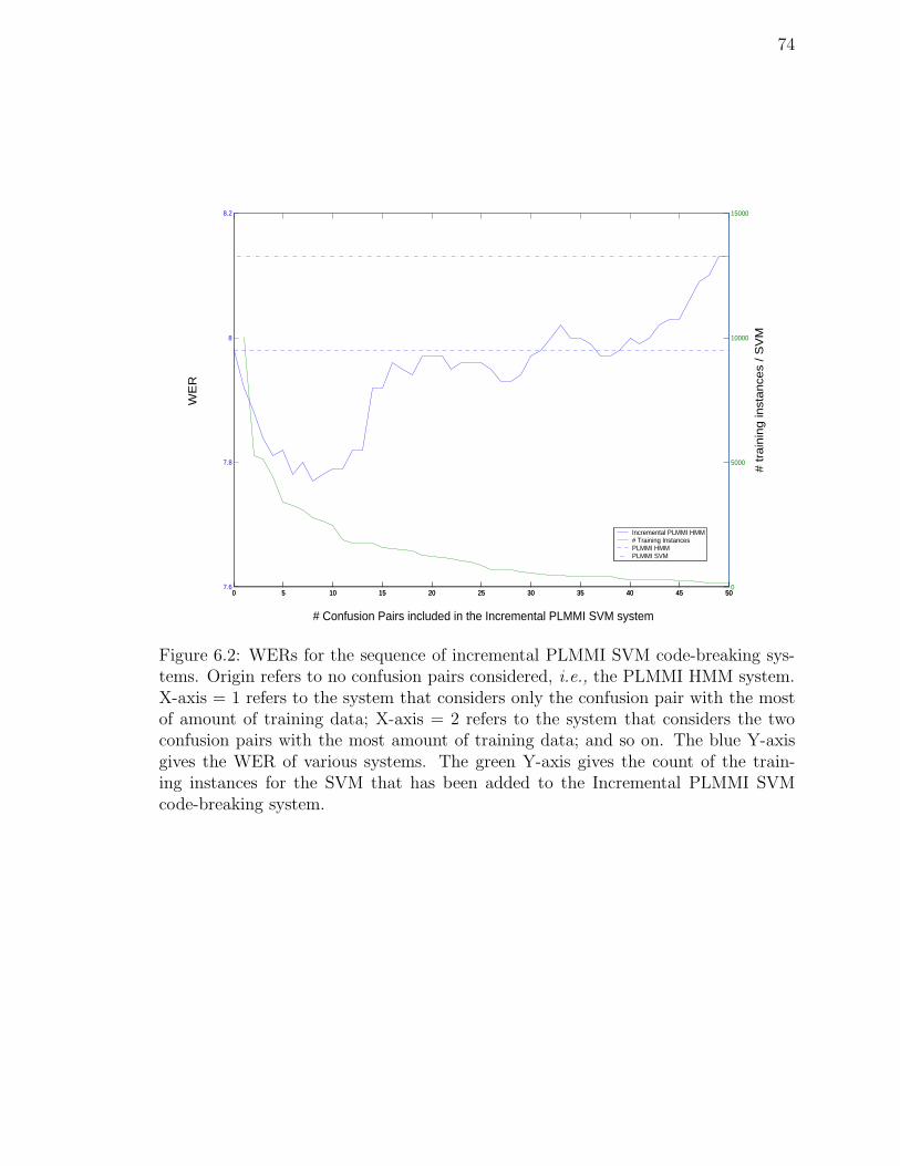
74

0 5 10 15 20 25 30 35 40 45 507.6

7.8

8

8.2

0 5 10 15 20 25 30 35 40 45 500

5000

10000

15000

Incremental PLMMI HMM# Training InstancesPLMMI HMMPLMMI SVM

# Confusion Pairs included in the Incremental PLMMI SVM system

WE

R

# tra

inin

g in

sta

nce

s / S

VM

Figure 6.2: WERs for the sequence of incremental PLMMI SVM code-breaking sys-tems. Origin refers to no confusion pairs considered, i.e., the PLMMI HMM system.X-axis = 1 refers to the system that considers only the confusion pair with the mostof amount of training data; X-axis = 2 refers to the system that considers the twoconfusion pairs with the most amount of training data; and so on. The blue Y-axisgives the WER of various systems. The green Y-axis gives the count of the train-ing instances for the SVM that has been added to the Incremental PLMMI SVMcode-breaking system.

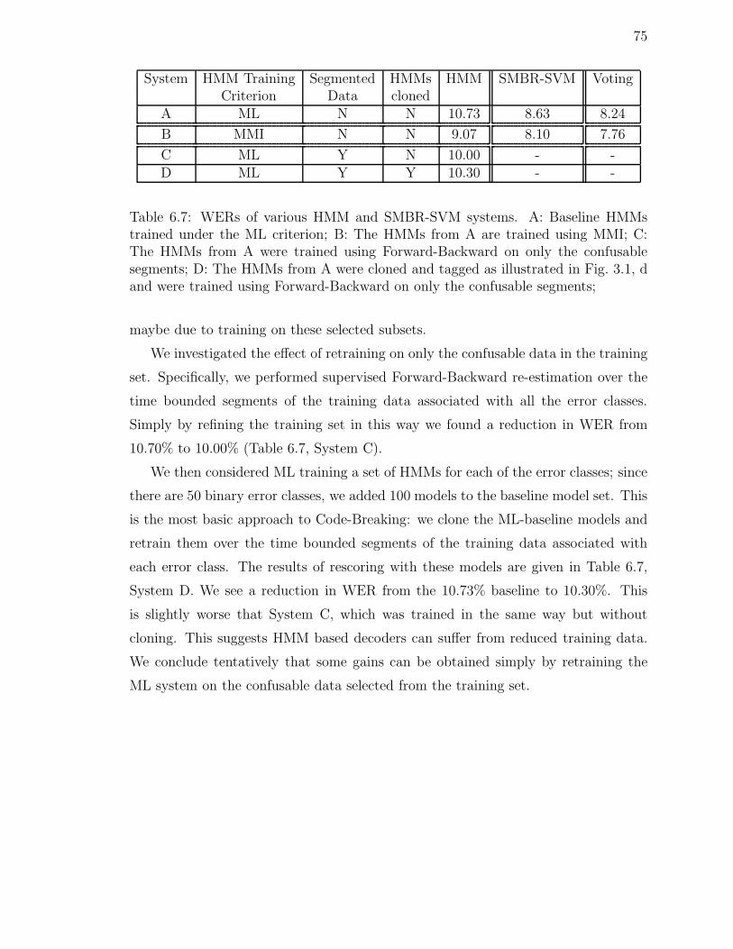
75

System HMM Training Segmented HMMs HMM SMBR-SVM VotingCriterion Data cloned

A ML N N 10.73 8.63 8.24

B MMI N N 9.07 8.10 7.76

C ML Y N 10.00 - -D ML Y Y 10.30 - -

Table 6.7: WERs of various HMM and SMBR-SVM systems. A: Baseline HMMstrained under the ML criterion; B: The HMMs from A are trained using MMI; C:The HMMs from A were trained using Forward-Backward on only the confusablesegments; D: The HMMs from A were cloned and tagged as illustrated in Fig. 3.1, dand were trained using Forward-Backward on only the confusable segments;

maybe due to training on these selected subsets.

We investigated the effect of retraining on only the confusable data in the training

set. Specifically, we performed supervised Forward-Backward re-estimation over the

time bounded segments of the training data associated with all the error classes.

Simply by refining the training set in this way we found a reduction in WER from

10.70% to 10.00% (Table 6.7, System C).

We then considered ML training a set of HMMs for each of the error classes; since

there are 50 binary error classes, we added 100 models to the baseline model set. This

is the most basic approach to Code-Breaking: we clone the ML-baseline models and

retrain them over the time bounded segments of the training data associated with

each error class. The results of rescoring with these models are given in Table 6.7,

System D. We see a reduction in WER from the 10.73% baseline to 10.30%. This

is slightly worse that System C, which was trained in the same way but without

cloning. This suggests HMM based decoders can suffer from reduced training data.

We conclude tentatively that some gains can be obtained simply by retraining the

ML system on the confusable data selected from the training set.

76

6.5 SVM Score-Spaces from Constrained Parame-

ter Estimation

We have studied a simple task so that we could develop the SMBR-SVM modeling

framework and describe it without complications. Our ultimate goal is to apply

this framework to large vocabulary speech recognition. Large vocabulary systems

typically consist of sub-word models that are shared across words. We could apply

the approach we have described thus far in a brute force manner by cloning the models

in the original large vocabulary HMM system and retraining them over confusion sets.

From systems C & D in Table 6.7 we saw there is value in retraining. However there

are some drawbacks to such an approach which we discuss in the following subsection.

6.5.1 Deriving Score-Spaces through Constrained Parameter

Estimation

Apart from the unwieldy size of a cloned system, the main problem with the brute

force approach of cloning models would be data sparsity in calculating statistics for

SVM training. This situation suggests the use of models obtained via constrained

estimation. We can use Linear Transforms (LT) such as Maximum Likelihood Linear

Regression (MLLR) [60] to estimate model parameters. Following the approach we

have developed, these transforms are estimated over segments in the acoustic training

set that were confused by the baseline system. We emphasize that the LTs are not

used as a method of adaptation to test set data.

Consider the case of distinguishing between two words in a large vocabulary sys-

tem. We need to construct models θ1 and θ2 from which we will produce the statistics

needed to train an SVM. We identify all instances of this confusion pair G in the train-

ing set and estimate two transforms L1 and L2 relative to the baseline HMM system.

These are trained via supervised adaptation e.g., MLLR. One approach is to derive

77

our Score-Space from the LT Score-Space is

ϕ(O) =

1

∇LG(1)

∇LG(2)

ln

(

p(O|LG(1) · θG(1))

p(O|LG(2) · θG(2))

)

. (6.2)

The LT Score-Space has attractive qualities. By using regression classes we can

control the dimensionality of the Score-Space. This will also allow us to address data

sparsity problems by clustering together similar error patterns into regression classes.

However, the Score-Space as found in Equation (6.2) was unsuitable for classification.

We hypothesize that since the LT scores can give no more than a direction in the

HMM parameter manifold, the SMBR-SVM system cannot build effective decision

boundaries in the LT Score-Space. When we inspected the kernel maps, we saw

no evidence of the block diagonal structure which would indicate features useful for

pattern classification.

An alternative is to create a constrained Score-Space by applying MLLR trans-

forms to original models to derive a new set of models. Our Score-Space is the original

mean Score-Space while the HMM parameters are modified by a LT estimated as de-

scribed above. If θ′G(i) = LG(i) · θG(i) and θ′ = [θ′G(1) θ′G(2)] then,

ϕ(O) =

[

1

∇θ′

]

ln

p(

O|θ′G(1)

)

p(

O|θ′G(2)

)

. (6.3)

Although intended for LVCSR, we investigated the feasibility of the approach in our

small vocabulary experiments. The results are tabulated in Table 6.8. We estimate

MLLR transforms with respect to the MMI models over the confusion sets. A single

transform was estimated for each word hypothesis in each confidence set. We then

apply the transforms to the MMI models and estimate statistics as described in

Equation (6.3). The performance is shown in Table 6.8, System B. We see a reduction

in WER with respect to the MMI baseline from 9.07% to 8.00%. We conclude that

the severely constrained estimation is able to generate Score-Spaces that perform at

similar WERs to those of unconstrained estimation. For completeness, we rescored the

confusions sets using the transformed MMI models. As can be expected performance

78

System HMMs HMM SMBR-SVMUsed

A MMI 9.07 8.10B MMI+MLLR 9.35 8.00

Table 6.8: WERs of HMM systems with and without MLLR transforms; SMBR-SVMsystems were trained in the Score-Space of the transformed models

degrades slightly from 9.07% to 9.35% suggesting that performing ML estimation

subsequent to MMI estimation undoes the discriminative training [73].

6.6 Summary of Experiments

This chapter presented experiments designed to validate the code-breaking frame-

work. We chose the Alphadigits corpus so that we could discuss the experiments

without complications. We found that for both the ML and the MMI HMMs, the

SVM code-breaking systems are able to substantially improve upon their respective

baseline systems. We are able to perform system combination based on the posterior

estimates from the HMM and SVM code-breaking systems to obtain further gains.

The PLMMI SVM code-breaking system performs comparably to the PLMMI HMM

system; training data sparsity was shown to be an issue for obtaining improvements

in this case. Upon system combination however, we are able to significantly improve

system performance. We also discussed various baseline HMM systems that result due

to the refinement in the training data. Finally we discussed constrained estimation

HMM systems towards implementing code-breaking in LVCSR tasks.

79

Chapter 7

Code-Breaking for Large

Vocabulary Continuous Speech

Recognition

The previous chapter described a set of experiments that showed how SVMs used

in a code-breaking framework can substantially improve the performance of an HMM-

based speech recognizer in low confidence regions. We showed improvements on top

of ML and MMIE trained HMMs and upon system combination over the PLMMI

HMMs. We also saw that in the case of PLMMI HMMs sparse training data can hurt

performance which indicated the need for a careful selection of confusion pairs as a

code-breaking set.

In this chapter we will first characterize confusion pairs that can arise in a large

vocabulary system. We will then describe the baseline system and the procedure to

obtain binary confusions. We will demonstrate the feasibility of the code-breaking

framework on a large vocabulary task by showing statistically significant improve-

ments relative to a baseline MMI system using SVMs. These descriptions will lead

to discussions on what challenges we face when we apply code-breaking on a large

vocabulary task. We will finally discuss approaches designed to obtain further im-

provements.

80

THEBEAR(b ey r)

BARE

DOG

(b ey r)

(d ao g)

THE(th ae)

(th iy)

BOG

(b ao g)

Figure 7.1: Examples of different kinds of confusions. Each path is labeled withboth the word and its phonetic sequence. left: a homonym confusion pair. center: anon-homonym confusion pair. right: a phonetic confusion pair.

7.1 Characterizing Confusion Pairs

In the previous chapter, we used lattice cutting techniques followed by pruning

(the greedy approach described in Section 3.2) to identify pairs of words that are

confusable. We defined the task so that only the acoustic model was relevant during

recognition. For a large vocabulary task all components of the recognizer play an

important role; ignoring any of them can lead to catastrophic degradation in per-

formance. Recall from Chapter 2 that some of the high level components of the

recognizer are the acoustic model that estimates P (O|B), the dictionary P (B|W )

and the language model that estimates P (W ), where O is the observations sequence

and B is a phonetic sequence of the word W . The difficulty in discriminating (cor-

rectly) between two words could have been due to short-comings in one of various

components of the baseline recognizer. This introduces several new challenges.

The first challenge is that lattice cutting does not directly tell us which compo-

nent of the recognizer could not distinguish (correctly) between the words. However,

a simple analysis of the confusable words and their baseforms can indicate which

component encountered difficulty in distinguishing words.

Let B1 and B2 be the phonetic sequence of the words W1 and W2 respectively. If B1

and B2 are the same for two distinct words (Figure 7.1, left), then the acoustic model

cannot distinguish between the two words. In fact any decoder that uses acoustic

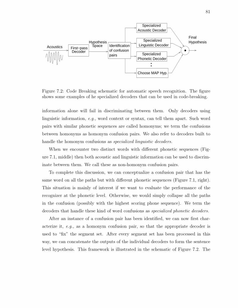
81

of confusionFirst−passDecoder

HypothesisSpace Identification

pairs

Acoustics

FinalHypothesis

SpecializedAcoustic Decoder

Linguistic DecoderSpecialized

Phonetic DecoderSpecialized

Choose MAP Hyp.

Figure 7.2: Code Breaking schematic for automatic speech recognition. The figureshows some examples of he specialized decoders that can be used in code-breaking.

information alone will fail in discriminating between them. Only decoders using

linguistic information, e.g., word context or syntax, can tell them apart. Such word

pairs with similar phonetic sequences are called homonyms; we term the confusions

between homonyms as homonym confusion pairs. We also refer to decoders built to

handle the homonym confusions as specialized linguistic decoders.

When we encounter two distinct words with different phonetic sequences (Fig-

ure 7.1, middle) then both acoustic and linguistic information can be used to discrim-

inate between them. We call these as non-homonym confusion pairs.

To complete this discussion, we can conceptualize a confusion pair that has the

same word on all the paths but with different phonetic sequences (Figure 7.1, right).

This situation is mainly of interest if we want to evaluate the performance of the

recognizer at the phonetic level. Otherwise, we would simply collapse all the paths

in the confusion (possibly with the highest scoring phone sequence). We term the

decoders that handle these kind of word confusions as specialized phonetic decoders.

After an instance of a confusion pair has been identified, we can now first char-

acterize it, e.g., as a homonym confusion pair, so that the appropriate decoder is

used to “fix” the segment set. After every segment set has been processed in this

way, we can concatenate the outputs of the individual decoders to form the sentence

level hypothesis. This framework is illustrated in the schematic of Figure 7.2. The

82

last block (“Choose MAP Hyp.”) in the list of decoders is for the high-confidence

segments that were identified and also for instances when none of the other decoders

come to a consensus.

The other issues involved in studying code-breaking on a large vocabulary system

will arise as we describe our experiments. We begin with a description of the corpus

we worked with and the HMM baseline system.

7.2 Baseline System Description

We evaluate our approach in the MALACH spontaneous Czech conversational do-

main [28]. The corpus consists of testimonials (or interviews) of Holocaust survivors.

There are around 350 interviews given in Czech, each around 2 hours long. Of this,

65 hours (24065 utterances) of transcribed speech from 336 interviews was selected

as the training set.

The baseline HMM system consists of speaker independent, continuous mixture

density, tied state, cross-word, gender-independent, triphone HMMs trained HTK-

style [27]. The speech was parameterized into 39-dimensional, MFCC coefficients,

with delta and acceleration coefficients. We used a bigram language model based on

a 83000 word vocabulary trained on the transcriptions of the interviews and interpo-

lated with web data as described in the paper by W. Byrne et al [28]. The AT&T

Large Vocabulary Decoder was used to generate lattices over the training and test

sets. Lattice-based MMI [102, 23] was then performed.

The test set consisted of ten testimonials from ten held-out speakers. There

were approximately 8400 utterances (≈ 25 hours of speech). Unsupervised MLLR

transforms for each of the ten test-set speakers were estimated on a 1000 utterance

subset of the test set. The baseline system produced a test set lattices with WER of

45.6% and 13.5% LER (listed in Table 7.1).

83

Lattices LER

One-best 45.6Baseline 13.5Pre-pinch (pruning links based on posteriors) 22.3Pinch and keeping NULL links 18.6Pinch and discarding NULL links 27.3

Table 7.1: LER of various lattices prior to and after pruning.

7.3 Lattice Pinching

We next proceed to pinching the test set lattices. We were not able to directly

pinch the baseline lattices at 13.5% LER. The reason is that the lattices have many

more links than those in the Alphadigits corpus and so the intermediate lattices

that are produced during pinching (steps 1 and 2 described in Section 3.1) become

prohibitively large. We therefore performed pruning of the links in the lattices based

on their posteriors (as defined in Equation 2.10). The LER for the set of the pruned

lattices was 22.3%, listed as ‘Pre-pinch’ in Table 7.1; these were the set of lattices

that were finally pinched.

The pinched lattices have an LER of 18.6%, listed as ‘Pinch and keeping NULL

links’ in Table 7.1. The decrease from 22.3% is due to pinching introducing additional

paths. Some of these additional paths are due to the NULL links in the segment sets.

We discard the NULL links since we want to focus on problems of choosing between

two words rather then choosing to delete words. Ignoring the NULL hypotheses from

the pinched lattices increases the LER to 27.3%. These are the lattices over which

we will attempt to find binary confusions.

7.4 Effectiveness of Segment Set Pruning

Let us assume we have restricted the pinched lattices to a sequence of binary

segment sets with utmost two paths, each one word long, as shown in Figure (7.3,

top). If we select an instance of a confusion pair to be ‘fixed’, we need to be fairly

confident that (a) the MAP hypothesis is actually wrong in that pair, and that (b)

84

V:5

B:5

A:7ASIL SIL

OH ASIL SILK

truth:

pinched lattices restricted to confusion pairs:

#5 #8#6#3 #4 #7#1 #2

9

9

B

4:23

OH:23

J:17

A:17

8:7

8

Figure 7.3: Labeling identified binary confusions as CPCOR or CPERR and as MAP-COR or MAPERR. The MAP hypothesis in the pinched lattice is shown in bold.Segments #2 and #6 are MAPCOR and CPCOR; segment #3 is MAPERR andCPERR; segment #7 is MAPERR and CPCOR.

the other hypothesis is actually the truth. While we found that both these issues

are manageable in small vocabulary tasks, in large vocabulary tasks, we face sparsity

issues due to the diversity of word confusions that arise; it may be difficult to ensure

the presence of the truth in a confusion pair. We now study the degree to which we

can ensure (a) and (b).

7.4.1 Evaluating the quality of a collection of Segment Sets

We first Levenshtein-align the confusion pair-only pinched lattices (Figure 7.3,

top) to the truth (Figure 7.3, bottom). We first count the number of Confusion Pair

Errors (CPERR), which are confusion pairs that do not contain the truth. For ex-

ample, in Figure 7.3, (A:17, J:17) is classified as CPERR since it does not contain

the true word ‘K’; the other sets are classified as Confusion Pair Oracle Correct (CP-

COR). While it is desirable to produce as few CPERR sets as possible, those CPERR

instances that do occur can be ignored. These are ‘lost causes’, where lattice pinching

failed to provide a good alternative and further processing can pick randomly from

the confusion pair without any meaningful effect on the overall WER.

The CPCOR segments are those which we are interested in. Within the CPCOR

segments we can distinguish those in which the MAP path agrees with the oracle

85

path (MAPCOR) and those in which the MAP path is in error (MAPERR). In

Fig. 3.1, d the pair (V:5, B:5) is classified as MAPERR, and the pairs (OH:23, 4:23)

and (A:7, 8:7) are MAPCOR; both these sets are CPCOR. It is desirable that we

do not create MAPCOR segment sets. We noticed that when we used the ‘greedy

approach’ (described in Section 3.2) to identify frequent confusion pairs, we had a

very high ratio of the number of MAPCOR segment sets to the number of MAPERR

sets.

We therefore studied another pruning strategy aimed at ensuring higher ratio

#MAPERR/#MAPCOR. Towards this we tried the ‘natural’ approach (described

in Section 3.2) for a range of thresholds. Table 7.2 gives the lattice error rate of

lattices for which the segment sets have been pruned to contain only paths that have

a posterior higher than the threshold. If we were to process these 27.3% LER lattices

with special-purpose classifiers, these classifiers would need to be able to distinguish

between 11.65 hypotheses on average, and if these classifiers were to perform perfectly,

they would lower the WER from 45.6% to 27.3%.

Since we wish to apply binary classifiers, the analysis at the 0.3 pruning threshold

of 0.3 is relevant, since, ‘on average’, pinching produces binary confusion pairs. While

the best performance that can be obtained is a WER of 43.2%, we stress that this

is improvement over a well-trained large vocabulary ASR system on a very difficult

test set.

7.4.2 Choosing the code-breaking set

We consider only those confusion pairs that occur in the test data at least 100

times. This is not a necessary restriction and it does further limit our potential

improvement, but it simplifies our analysis in that there are enough instances of each

pair to reliably measure recognition performance over each of them. Referring to

Figure 7.3, top, only these frequently occurring confusion pairs are retained, and all

others are pruned back to the primary hypothesis.

We further process the pinched lattices constructed from the frequently occurring

confusion pairs. We renormalize these lattices to define the posterior distribution

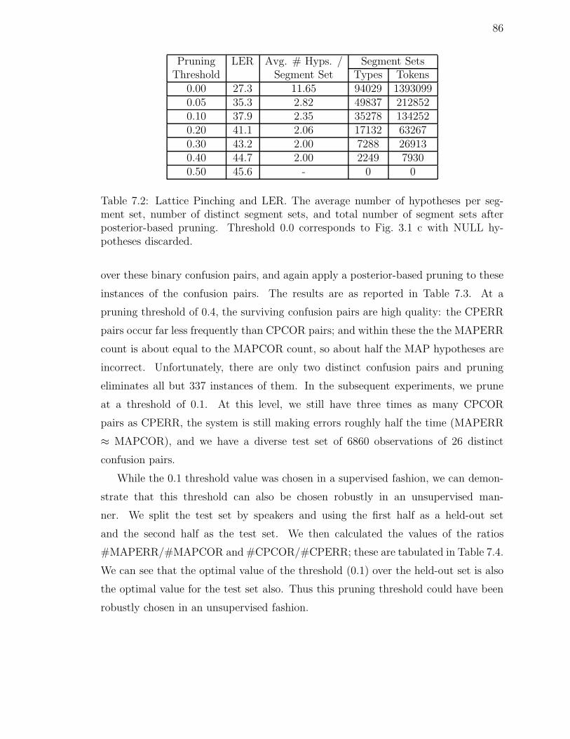
86

Pruning LER Avg. # Hyps. / Segment SetsThreshold Segment Set Types Tokens

0.00 27.3 11.65 94029 13930990.05 35.3 2.82 49837 2128520.10 37.9 2.35 35278 1342520.20 41.1 2.06 17132 632670.30 43.2 2.00 7288 269130.40 44.7 2.00 2249 79300.50 45.6 - 0 0

Table 7.2: Lattice Pinching and LER. The average number of hypotheses per seg-ment set, number of distinct segment sets, and total number of segment sets afterposterior-based pruning. Threshold 0.0 corresponds to Fig. 3.1 c with NULL hy-potheses discarded.

over these binary confusion pairs, and again apply a posterior-based pruning to these

instances of the confusion pairs. The results are as reported in Table 7.3. At a

pruning threshold of 0.4, the surviving confusion pairs are high quality: the CPERR

pairs occur far less frequently than CPCOR pairs; and within these the the MAPERR

count is about equal to the MAPCOR count, so about half the MAP hypotheses are

incorrect. Unfortunately, there are only two distinct confusion pairs and pruning

eliminates all but 337 instances of them. In the subsequent experiments, we prune

at a threshold of 0.1. At this level, we still have three times as many CPCOR

pairs as CPERR, the system is still making errors roughly half the time (MAPERR

≈ MAPCOR), and we have a diverse test set of 6860 observations of 26 distinct

confusion pairs.

While the 0.1 threshold value was chosen in a supervised fashion, we can demon-

strate that this threshold can also be chosen robustly in an unsupervised man-

ner. We split the test set by speakers and using the first half as a held-out set

and the second half as the test set. We then calculated the values of the ratios

#MAPERR/#MAPCOR and #CPCOR/#CPERR; these are tabulated in Table 7.4.

We can see that the optimal value of the threshold (0.1) over the held-out set is also

the optimal value for the test set also. Thus this pruning threshold could have been

robustly chosen in an unsupervised fashion.

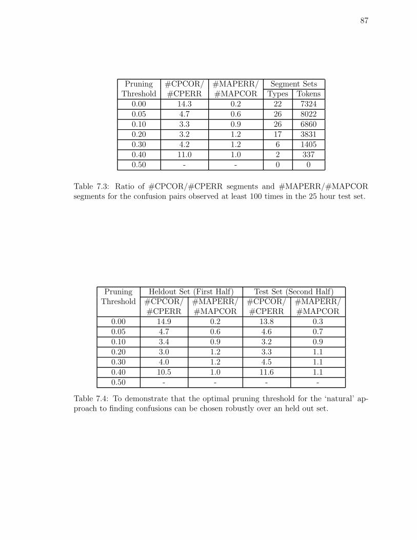
87

Pruning #CPCOR/ #MAPERR/ Segment SetsThreshold #CPERR #MAPCOR Types Tokens

0.00 14.3 0.2 22 73240.05 4.7 0.6 26 80220.10 3.3 0.9 26 68600.20 3.2 1.2 17 38310.30 4.2 1.2 6 14050.40 11.0 1.0 2 3370.50 - - 0 0

Table 7.3: Ratio of #CPCOR/#CPERR segments and #MAPERR/#MAPCORsegments for the confusion pairs observed at least 100 times in the 25 hour test set.

Pruning Heldout Set (First Half) Test Set (Second Half)Threshold #CPCOR/ #MAPERR/ #CPCOR/ #MAPERR/

#CPERR #MAPCOR #CPERR #MAPCOR0.00 14.9 0.2 13.8 0.30.05 4.7 0.6 4.6 0.70.10 3.4 0.9 3.2 0.90.20 3.0 1.2 3.3 1.10.30 4.0 1.2 4.5 1.10.40 10.5 1.0 11.6 1.10.50 - - - -

Table 7.4: To demonstrate that the optimal pruning threshold for the ‘natural’ ap-proach to finding confusions can be chosen robustly over an held out set.

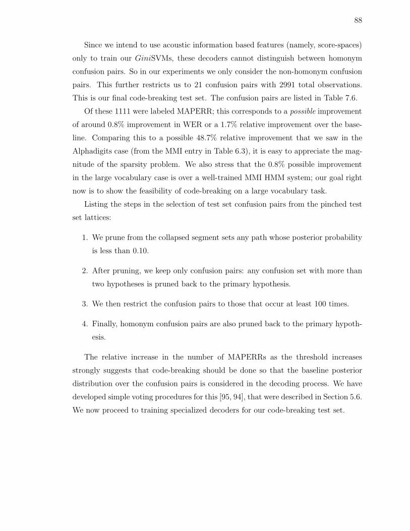
88

Since we intend to use acoustic information based features (namely, score-spaces)

only to train our GiniSVMs, these decoders cannot distinguish between homonym

confusion pairs. So in our experiments we only consider the non-homonym confusion

pairs. This further restricts us to 21 confusion pairs with 2991 total observations.

This is our final code-breaking test set. The confusion pairs are listed in Table 7.6.

Of these 1111 were labeled MAPERR; this corresponds to a possible improvement

of around 0.8% improvement in WER or a 1.7% relative improvement over the base-

line. Comparing this to a possible 48.7% relative improvement that we saw in the

Alphadigits case (from the MMI entry in Table 6.3), it is easy to appreciate the mag-

nitude of the sparsity problem. We also stress that the 0.8% possible improvement

in the large vocabulary case is over a well-trained MMI HMM system; our goal right

now is to show the feasibility of code-breaking on a large vocabulary task.

Listing the steps in the selection of test set confusion pairs from the pinched test

set lattices:

1. We prune from the collapsed segment sets any path whose posterior probability

is less than 0.10.

2. After pruning, we keep only confusion pairs: any confusion set with more than

two hypotheses is pruned back to the primary hypothesis.

3. We then restrict the confusion pairs to those that occur at least 100 times.

4. Finally, homonym confusion pairs are also pruned back to the primary hypoth-

esis.

The relative increase in the number of MAPERRs as the threshold increases

strongly suggests that code-breaking should be done so that the baseline posterior

distribution over the confusion pairs is considered in the decoding process. We have

developed simple voting procedures for this [95, 94], that were described in Section 5.6.

We now proceed to training specialized decoders for our code-breaking test set.

89

7.5 Training Specialized Decoders

The next step is to use the baseline HMMs we have trained, generate scores for

the segment sets and then decode with SVMs. However, unlike in the Alphadigits

task, our baseline HMMs now are cross-word triphone models; not word-level models.

This introduces a complication for generating scores. Recall that the score for an

observation O for a confusion pair between the words w1 and w2 is defined as

ϕ(O) =

ln p(O|θ1)p(O|θ2)

∇θ1 ln p(O|θ1)

−∇θ2 ln p(O|θ2)

(7.1)

where θi are the HMM parameters representing the word wi. If we use cross-word

triphone models, the HMMs representing a word and thus θ changes with its context.

So the score-space becomes context dependent. While it may be desirable to account

for the context during modeling, it would greatly complicate the approach. We bypass

this context issue by training special purpose word-level HMMs for the words in the

confusion pairs. This fixes the score space for every instance of each confusion pair.

7.5.1 Training Acoustic HMMs

A set of 12 Gaussian mixture 3 state monophone HMMs are trained over the 65

hours of acoustic training set, and these models are also used to align the training set.

Whole-word acoustic models for the words in confusion pairs are initialized with these

monophone models; the number of states for each of these word models depends on

the number of phones in the dictionary entry for the word, e.g., the baseform sequence

for the word TAM had 3 phones, so the initialized word model is a 9 state HMM.

The word models are then then reestimated using Baum Welch over word segments

extracted from the aligned training set.

We next clone these whole-word models for the confusion pairs, e.g., referring to

Figure (7.3, top), the model for the word ‘A’ is replicated so that A:17 and A:7 are

two different whole-word HMMs. To train discriminative models for a confusion pair,

say (w1, w2), we create a special confusion pair training subset using the “transcrip-

90

tion based confusions” method described in Section 3.4. This subset consists of all

instances of the words w1 and w2 in the original training set along with their acoustic

segments. The label for each segment is of course the word spoken. We term the

new training set created for all the confusion pairs collectively as the “confusion pair

training set”.

Two iterations of MMI is then used to further train the cloned models, say, A:7

and 8:7 over its corresponding training subset. This process is repeated for all of the

confusion pairs, and in this way, the models are specialized to discriminate between

the words in the confusion pairs. Throughout all this we keep track of pronunciation

variation. For example, the word ‘TAK’ has pronunciations t a k and t a g, and

the word ‘PAK’ has only the pronunciation p a k. Models are trained for all three

instances, and t a k vs. p a k and t a g vs. p a k would be considered as two

distinct confusion pairs.

Models Training Error RateBaseline MMIE Triphone 11.1

Word level ML 20.0Word level MMI 13.8

GiniSVMs 7.9

Table 7.5: Performance of various models when evaluated on the ‘confusion pairstraining set’ created to train MMI word level HMMs. The hypothesis of each modelfor each segment set was taken to be the word that was assigned an higher likelihood.No language model information is used during this evaluation.

The performance of these MMI trained word-level HMMs on the confusion pairs

training set are listed in Table 7.5. The decoding for each confusion pair was carried

as follows: for an instance of a confusion pair, we calculate the likelihood of the

acoustic segment under the HMM sequence representing each word; the hypothesis

chosen for each segment set is the word with the higher likelihood. No language

model is used during this evaluation. We can see that while MMI training does

improve the performance of the ML trained word-level HMMs, they do not show

better performance than the baseline triphone models. Further iterations of MMI did

improve the error rate although not substantially; the models were not able to match

91

the baseline models either.

For decoding on the code-breaking test set, we applied the MMI-trained word-level

HMMs to each segment set to choose a second-pass hypothesis. We then obtain the

utterance level hypothesis by replacing each segment with the second-pass hypothe-

sis. However, we noticed a degradation in performance compared to the 45.6%WER

baseline. System combination schemes between the MMI-trained word-level HMM

system and the original baseline system did not help either.

7.5.2 Training Acoustic SVMs

We now have all that is needed to train acoustic SVMs for the confusion pairs.

the GiniSVM toolkit [13] was used to train SVMs for the 21 non-homonym confusion

pairs. The MMI trained word HMMs were used to generate mean and likelihood-ratio

scores.

The amount of training data for each confusion pair depends on the frequency

of words that make up the confusion pair. Therefore confusions between the most

frequent words in the training set may be associated with large amounts of training

data; e.g., there were a total of more than 30,000 occurrences of the words A and TO.

So the confusion pair A vs. TO would be associated with these many training tokens.

It was not practical to train SVMs on such large amounts of data. To train SVMs

for these confusion pairs, we filtered out data: we first estimate log-likelihoods of the

hypotheses in a segment set using the word-level MMI trained HMMs and converted

them into posteriors. Only those segments for which the models assigned a posterior

of < 0.99 for the true hypothesis were taken as training tokens.

All SVMs were trained in 20% of the most informative dimensions (as chosen using

Equation 5.20). We noticed that performace of the SVMs was stable for a range of

dimensionalities of the score-space used (15% to 25%); thus a held-out set could have

been used to determine the optimal dimensions to use. We used the tanh kernel and

a global SVM trade-off parameter of 1.0 for all the confusion pairs.

For the evaluation of the SVMs on the confusion pairs training subset, the label

with the higher posterior probability was chosen as the output for each training token.

92

0 1 2 3 4 5 6 7 8 9 10 11 12 13 14 15 16 17 18 19 20 210

20

40

60

80

100

120

140

160

180

Index of Confusion Pair

Error Counts

MAPSVMMAP+SVM

Figure 7.4: Error counts over individual confusion pairs. The confusion pair withtheir indices are listed in Table 7.6

We can see from Table 7.5, the trained SVMs not only improve upon the MMI word-

level HMMs, but they also improve upon the baseline HMMs.

On the code-breaking test set, we performed decoding similarly as in the case of the

MMI-trained word-level HMMs. We did notice a 0.1% improvement over the 45.6%

WER baseline; unfortunately, this improvement was not found to be statistically

signifcant.

For each of the 21 confusion pairs, Figure 7.4 reports performance of the baseline

HMM system, the SVM decoders, and a hybrid decoder combining the two. The

baseline performance over each confusion pair is the left-most of each of the three

bars. The decision is made simply by picking the most likely alternative under the

lattice posterior; this likelihood is based on the triphone HMM acoustic score, with

MLLR, and the bigram language model. An error occurs when picking the wrong

word relative to the Levenshtein alignment of the pinched lattice to the truth; e.g.,

in Fig. 3.1 d, picking V:5 would count as an error.

For each confusion pair instance, the appropriate discriminatively trained whole-

word was used to create score-space features for use in classification by the SVM

trained for that pair. The performance over each of the 21 confusion pairs is given in

the center bars of the plots in Fig. 7.4. Performance relative to the MAP baseline is

mixed; there are not consistent improvements.

93

Index Confusion Pair Phonetic levelword 1 word 2 Baseform 1 Baseform 2

1 TAM TO t a m t o

2 SE SI s e s i

3 SE SEM s e s e m

4 JA A j aa a

5 BYLA BYLO b i l a b i l o

6 NO NA n a n o

7 NO A a n o

8 NA A a n a

9 TA TO t a t o

10 TU TO t u t o

11 BYL BYLO b i l b i l o

12 A TO a t o

13 A ALE a a l e

14 TO TOHO t o t o h o

15 PAK TAK p a k t a k

16 DY KDY d i sh g d i sh

17 TIM TIM tj i m tj ii m

18 MYSLIM MYSLIM m i s l i m m i s l ii m

19 NEVIM NEVIM n e v i m n e v ii m

20 TY TY t i t ii

21 ETI JETI e sh tj e j e sh tj e

Table 7.6: Confusion Pairs and their Indices listed in Figure 7.4

94

7.5.3 SVM-MAP Hypothesis Combination

To combine the SVM and MAP decisions, we use the posterior distribution over

the SVM decisions estimated by logistic regression [94]. For a particular instance

of a confusion pair with words (w1, w2), let ph(w) be the MAP posterior over the

pinched lattices, and ps(w) be the SVM confidence in each decision. A simple linear

interpolation

pλ(wi) = λph(wi) + (1 − λ)ps(wi)

where 0 ≤ λ ≤ 1, and i ∈ 1, 2, gives a combined likelihood over the word pair.

With λ = 0.5, the performance over the 21 pairs by this SVM-MAP combination

system is given in the third of the bars in Fig. 7.4. Under this combination, the error

count decreases in 18 of the 21 pairs.

The influence of these reductions on the overall WER over the complete 25 test set

is necessarily limited, for the reasons already discussed. The main reason is that the

2991 words in the code-breaking test set are only a small portion of the complete

25 hour test set. Under the MAP-SVM combination system, the baseline MAP

WER is reduced from 45.6% to 45.5%. However small, these gains are statistically

significant and stable with respect to λ: we obtained this performance improvement

for λ = 0.4, 0.5, 0.6, and, 0.7, and in all instances the significance test p-values [78]

were less than 0.001.

7.6 Summary of Experiments

The experiments in this chapter were designed to show the feasibility of code-

breaking on an LVCSR task. We showed that we can use GiniSVMs in combination

with the baseline HMM system to give statistically significant improvements. We dis-

cussed several challenges in studying code breaking on an LVCSR task; our methods

to handle these challenges decreased the potential gains from the framework. This

lead to the final potential gains being modest. However, this does not reflect any

insurmountable limitation in the approach.

Expanding the code-breaking test set, possibly by more permissive pruning and

95

acoustic clustering of confusion sets, will provide opportunity for greater improve-

ments. We only have to ensure that the ratio #MAPERR/#MAPCOR remains

favorable. We will now briefly discuss clustering confusions.

96

Chapter 8

Clustering and MLLR Techniques

for Pronunciation Modeling

We saw in Chapter 7 that it is possible to use the code-breaking framework in a

large vocabulary task to improve the performance of a HMM-based speech recognizer.

A system combination scheme using the posterior estimates from GiniSVMs together

with the estimates from the baseline HMM system led to statistically significant

improvements. The main reason for our modest gains was the size of the code-breaking

test set; it was necessarily small since we only considered the most frequently occurring

word-level confusion pairs. Since sparsity was severe, these frequent confusion pairs

did not account for a significant number of errors made by the baseline system.

The potential gains can possibly be made larger by expanding the code-breaking

test set. We will now investigate clustering confusions to increase the size of the

code-breaking test set.

8.1 Clustering Confusions

Clustering schemes can be used to group confusions that arise due to a specific

change in acoustics e.g., the presence or absence of voicing in a word. Assume that

we have a robust voicing detector available. All the grouped confusions can then be

resolved by this specialized voicing decoder. Consider the confusions, SINK vs. ZINC

97

and SAP vs. ZAP with the dictionary entries:

SINK s ih ng g SAP s ah p

vs. vs.ZINC z ih ng g ZAP z ah p.

In our earlier approach, we would have trained two separate decoders to distinguish

between the words in the two confusions. By clustering at the phonetic level, we can

account for both the confusion pairs with one decoder. Thus by clustering we will be

able to expand our code-breaking test set.

If these acoustic changes can be captured consistently and reliably, we can then

create classes of different acoustic changes. Each of these acoustic classes can also

be modeled robustly. We have investigated one clustering scheme that captured the

change in manner and place of articulation of vowels. The goal was to account for as

much of the pronunciation variation as possible in a corpus. This study was in the

context of pronunciation modeling and we will present this in the rest of this chapter.

8.2 Modeling Pronunciation Variation

Spontaneous and casual speech exhibits a high degree of variation in pronunciation

compared to read speech. The canonical pronunciations found in the dictionary are

not sufficient to model these variations. Pronunciation modeling for ASR provides

a mechanism by which ASR systems can be adapted to accented, spontaneous, or

disfluent speech. It is reasonable to expect that a speaker will chose to pronounce the

word IT as ih d rather than ih t or that the words GOING TO as a single entity

pronounced as g uh n ah.

One aspect of this modeling problem is to build predictive or descriptive models

for phenomena of interest that can predict surfaceform pronunciation (the sequence

of phones actually spoken) given the baseform or canonical pronunciation. Methods

are available that can learn and predict the surfaceform pronunciations given their

canonical baseforms [82].

Once these predictive models are trained they can be incorporated directly into

an ASR system. For the purposes of this section, we will augment the notation of the

98

acoustic models as P (O|B; θB) that assign likelihood to the acoustic observations O

given the baseforms B. The notation θB indicates that the acoustic model parameters

were trained using baseform transcriptions of the acoustic training set. The pronunci-

ation model is assumed to be available as a distribution P (S|B) that maps baseforms

to surfaceform sequences S; frequently used techniques such as augmenting a lexicon

with frequent pronunciation alternatives or decision trees that map baseform phone

sequences to surfaceform sequences [9] can be described in the following way. The

maximum likelihood decoder can be stated as

argmaxW,S,B

P (O|S, B)P (S|B)P (B|W )P (W ) (8.1)

if appropriate conditional independent assumptions are made.

In addition to the pronunciation model, a particular form of acoustic model

P (O|S, B) is needed. A simple approximation is available as P (O|S, B) ≈ P (O|S; θB),

where acoustic models trained on baseform transcriptions are used directly with the

surfaceform sequences produced by the pronunciation model. The ASR system is

therefore able to produce word hypotheses based on pronunciations not present in the

original dictionary. This straightforward approximation is especially effective because

it allows the pronunciation model to be incorporated into the ASR system without

retraining the ASR acoustic models. However since the acoustic models used in this

approximation were trained on the baseform pronunciations, the recognition process

is inevitably biased towards word hypotheses based on canonical pronunciations.

This observation leads to another aspect of the pronunciation modeling problem

which is to incorporate models of pronunciation variability directly into acoustic mod-

eling. Interestingly, it has been found that straightforward approaches to this problem

often fail. One possible approach would be to train a pronunciation model; verify that

it works well when used with a standard ASR system (by using the approach described

in the previous paragraph); use this pronunciation model to retranscribe the acoustic

training set to obtain a surface form transcription; retrain the acoustic models; and

evaluate the new ASR system with the pronunciation model. This approach yields a

set of models with parameters θS which can also be used to approximate P (O|B, S)

as P (O|S; θS). However, as has been discussed by M. Saraclar and S. Khudanpur [87],

99

this can lead to degradation in ASR performance. M. Saraclar and S. Khudanpur

conclude that it is incorrect to approximate P (O|S, B) by either P (O|S; θB) or by

P (O|S, θS). They demonstrate that when a base phone b is realized as a surfaceform

s, the acoustic model should model it as such, i.e., it should model it not as an s but

as a particular variant of b. In other words, surfaceforms should not be modeled with-

out consideration of the baseform from which they originate. In terms of modeling,

P (O|S, B) should retain dependencies on both baseform and surfaceform.

8.3 MLLR Pronunciation Modeling

We will use acoustic model adaptation techniques to approximate the distribution

P (O|S, B) by transforming the parameters of the baseform ASR system P (O|B; θB).

We assume that a surfaceform transcription of the acoustic training data is available,

either from human annotators or through forced alignment using the pronunciation

model and the acoustic models θB . We then align the surface annotations to the base-

form transcriptions using a phonetic feature distance [82]. This symbol-to-symbol

alignment allows us to construct a hybrid transcription for the training data: the

original baseform sequence bj after alignment with the surface sequence sj be-

comes bj :sj. This hybrid transcription is used in supervised MLLR adaptation to

estimate transforms TS,B that are applied to the parameters of the baseform models

to make the approximation P (O|S, B) ≈ P (O|TS,B · θB).

However, this increased resolution in acoustic modeling introduces complications.

The number of pairs b:s is potentially large; for a phone set of size 50, it is 2500.

This means insufficient training data to train the transforms TS,B robustly. We use

Phonetic transform regression classes are used to model the pairs b:s. Suppose an

instance of the words SUPPOSE ITS with baseform transcription s ax p ow z ih

t s has the surfaceform annotation s ih p ow s ih d z. After alignment the hy-

brid transcription becomes s:s ax:ih p:p ow:oh z:s ih:ih t:d s:z. A set of

100

phonetic transformation regression classes could be defined as

Tb,s =

TI s = b, no change

Tvoice+ b unvoiced, s voiced

Tnasal− b nasal, s not nasal

. . .

In the examples given here, the transform Tvoice+ is trained on all data whose

annotation indicates that an unvoiced baseform has changed to a voiced surfaceform,

for example data labeled as s:z or p:b.

Through the choice of regression classes we can adapt the models to the amount

of available data or the expected phonetic variability. For example, it may be that

consonants are observed to have little surfaceform variation, so regression classes

might be constructed to describe only vowel variation. The classes need not be

entirely complementary. For example, classes Tvoice+ and Tplosive:voice+ could coexist.

Instances of both p:b and s:z would be used to train the former, whereas instances of

s:z would not be used to train the latter. This allows a hierarchy of transforms that

can be applied depending on the amount of training data available for each regression

class.

The transform TI associated with the no change phonetic transformation class is

also estimated since the hybrid classes should be purer than the original baseform

phonetic classes. For example, if an acoustic model was to be trained for p:p, all

instances of p:t and other surfaceform variants would be excluded from training.

This more homogeneous training set allows sharper acoustic models to be trained

even for cases when no surfaceform variations are observed.

8.3.1 Review of Prior Work

We note that adaptation techniques have been used before for pronunciation mod-

eling. In dialect adaptation [25, 47] or in training a speaker dependent ASR system it

is possible to use MAP or other acoustic adaptation techniques to refine the models to

the new domain. It is assumed that sufficient data is available that the existing dic-

tionary and model architecture are able to model the regular and consistent variations

101

found in the data. A predictive model of pronunciation change was not incorporated

into acoustic model adaptation; i.e., the canonical dictionaries were used without

change. The goal of this work is to explore the coupling of predictive pronunciation

models with these acoustic adaptation techniques.

8.4 Pronunciation Modeling Experiments

In the experiments we discuss here we focus on the prediction of surface pronun-

ciations given the word sequence

argmaxS,B

P (O|S, B)P (S|B)P (B|W ). (8.2)

This paradigm isolates the prediction of phonetic variation from the larger problem

of incorporating pronunciation models into an ASR system with the goal of reducing

word error rate. Performance is measured relative to phonetic transcriptions provided

by expert phoneticians. We use the test and training set definitions and evaluation

procedures established for the phonetic evaluation component of the 2000 Large Vo-

cabulary Conversational Speech Recognition evaluation [35] that makes use of the

ICSI phonetically transcribed SWITCHBOARD collection [45].

Baseform acoustic models P (O|B; θB) consisting of 48 monophone models were

trained as in the JHU 2000 evaluation system [35]. The models were estimated

on the training portion of the ICSI data using the phonetic transcription obtained

from the lexicon; we note that monophone models have been found to be better for

the prediction of surface variation than triphones. Each model was a three state

left-to-right HMM with an 8 mixture, diagonal covariance Gaussian output density

trained using HTK [27]. Surfaceform monophone acoustic models P (O|B; θS) with

the same structure were also trained on the same data using the ICSI surfaceform

transcriptions.

The decision tree pronunciation model [82] used to approximate P (S|B) was based

on the JHU 2000 phonetic evaluation system [35]. The models were trained on the

training portion of the training set and incorporated only intra-word phonetic context;

cross-word phonetic context was not used.

102

Acoustic Model Phone Error Rate (%)Baseform 21.75

Surfaceform 20.50

Table 8.1: Baseform and Surface Acoustic Model Performance.

The availability of the surfaceform and baseform acoustic models allow us to

approximate P (O|S, B) in Equation 8.2 as either P (O|θS) or P (O|θB). The pronun-

ciation model was applied to the test set word transcriptions to generate lattices of

pronunciation alternatives for the test set utterances. As reported by M. Saraclar [86],

the surface-form trained acoustic models gave the best phone error rate relative to

the reference ICSI test set transcriptions (Table 8.4).

To train the MLLR transforms to be used as pronunciation models a surfaceform-

tagged baseform transcription of the training set was produced by a symbolic align-

ment of the baseform transcriptions to the surfaceform transcriptions using phonetic

feature distances [82]. For given sets of regression classes, each regression class trans-

form was trained with six iterations of MLLR. Only mean transforms were estimated.

Tagged lattices were created from the lattices of pronunciation alternatives by

tagging each surfaceform lattice link by the baseform phone from which it originated.

Deletion arcs were left untouched. Only two instances of insertion were modeled:

en → en n and el → el l. After MLLR transform estimation, decoding was done

on the tagged-test-set lattices. Transforms were applied to the baseform acoustic

models according to the regression class of each tagged lattice link. Viterbi rescoring

of the lattice yields a string of tagged phones; the surfaceform tag sequence is the

hypothesis.

We report results using phonetic transformation regression classes based on the

vowel groupings listed in Table 8.2. Regression classes based on consonant changes

yielded very little improvement when used alone and had little effect when used along

with vowel change regression classes. This is consistent with the observed behavior

of both the baseform and surfaceform phone recognition systems which recognize

consonants more reliably than vowels.

103

Class Phones Class Phonesfl ae ch ix ux

fml eh bl aa ay aw

fmh ih ey er bml ao ow oy

fl iy y bmh uh

cml ah ahi bh w uw

cmh ax el en ax em v all vowels

Table 8.2: Base Acoustic Classes Used to Construct Phonetic Transformation Re-gression Classes. Classes are based on vowel manner and place of articulation: front,central, back, high, middle, low.

Figure 8.1 shows the regression tree with the phonetic transformation classes used

in these MLLR pronunciation modeling experiments. The v2f (vowel2front) label, for

example, associated with node 10 specifies a regression class for baseform - surfaceform

pairs b:s such that b is a vowel and s is a front vowel. The regression tree node indices

also give the order in which the regression classes were created.

Performance was also found to be very sensitive to the choice of regression classes.

For example, if vowel2central is included as a regression class, there is no improvement

in PER unless central2central is also included as a regression class.

For comparison purposes, we built regression trees using the routines provided

by the HTK 3.0 Toolkit [27]. Relatively little improvement over the baseline was

observed.

Recognition results that show that phone error rate improves as phonetic trans-

formation classes are added are given in Table 8.3. As more classes are added perfor-

mance approaches that of acoustic models trained directly on surface form transcrip-

tions. Clearly, enough classes can be added so that each state, and eventually each

Gaussian component, will be trained individually and surfaceform acoustic models

will result. In these simple experiments we do not expect an improvement over the

surfaceform models, as the corpus is fairly homogeneous and there is sufficient data

to train each individual surfaceform model. These experiments demonstrate however

that phonetic transformations defined in terms of broad acoustic classes are able to

capture nearly all of the predictive gains that can be obtained using detailed acoustic

104

2 3

1

4 5

6 7 8 9

sil

nochange

vow

v2cml v2f

v2fmh

v2fh v2bl

v2bml

v2bl

v2c

14 15 10 11

16 17 12 13

18 19 20 21

22 23

Figure 8.1: Phonetic Transformation Regression Tree. The symbols are elaborated inTable 8.2

models trained on surfaceform transcriptions.

8.5 Conclusions

We have shown that it is feasible to use MLLR transforms to model the pronunci-

ation variation between the baseforms and surfaceforms at the acoustic level. Ideally

the application of this approach will allow a hierarchy of phonetic transformation

classes to be defined in which individual baseform-surfaceform pairs are assigned to

the most appropriate class based on acoustic similarity. We hope that these tech-

niques will allow for the development of procedures that improve the adaptation of

ASR systems to new speakers and dialects.

More relevant to this thesis, however, we showed that we were able to create

phonetic transformation regression classes that captures acoustic changes with specific

phonetic features. These changes were noticed consistently and reliably for us to

model the acoustics. It is hoped that these kind of techniques can be used to cluster

confusions to build robust phonetic feature detectors and incorporate them in the

code-breaking framework.

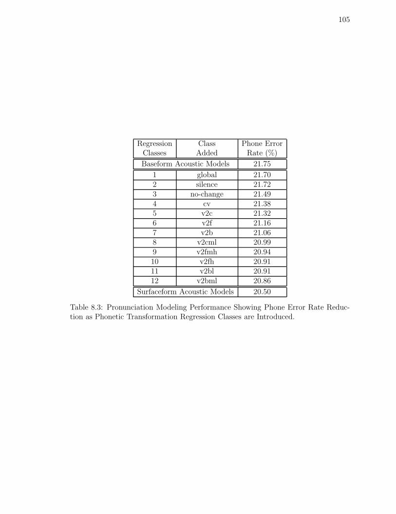
105

Regression Class Phone ErrorClasses Added Rate (%)

Baseform Acoustic Models 21.75

1 global 21.702 silence 21.723 no-change 21.494 cv 21.385 v2c 21.326 v2f 21.167 v2b 21.068 v2cml 20.999 v2fmh 20.9410 v2fh 20.9111 v2bl 20.9112 v2bml 20.86

Surfaceform Acoustic Models 20.50

Table 8.3: Pronunciation Modeling Performance Showing Phone Error Rate Reduc-tion as Phonetic Transformation Regression Classes are Introduced.

106

Chapter 9

Conclusions

In this final chapter, we first list some possible directions for future work. We

then layout the contributions of this thesis.

9.1 Directions for Future Work

There are several directions in which we could extend the work presented in this

thesis. We briefly discuss two of them here.

9.1.1 Language Model Code Breaking

In all our experiments, the specialized decoders used only acoustic information.

This need not be the case; we can build decoders that depend only on linguistic

information or decoders that use both kinds of information [38]. We will briefly

consider specialized language model decoders here.

Let C = w1, w2 be a confusion pair. Assume we have identified tokens of the

confusion pair in the transcriptions used for training the recognizer. We can create a

training set wil,w

ir, w

iNi=1 consisting of the complete string of words on both the left

and the right context for each of the N instances of C, where wi ∈ C are the truth

labels. For each instance of the confusion pair we can associate features Φ based on

the syntactic context e.g., the preceding or succeeding n-gram sequence, the parse

107

tree structure for the utterance and so on. This results in a feature-based training set

Φi, wiNi=1 using which we can estimate a probability distribution P (w|Φ), w ∈ C,

possibly using GiniSVMs.

For each instance of the confusion pair C in the test set with features Φ, the

hypothesis w will be chosen based on the estimated distribution, i.e.,

w = argmaxw∈C

P (w|Φ) (9.1)

This is an explicit form of building language models to discriminate between spe-

cific word pairs. This is in contrast to earlier work [83] where language model weights

in large lattices were modified to reduce the WER.

9.1.2 Multi-Class classifiers

An immediate extension to our experiments towards obtaining further improve-

ments is the use of multi-class classifiers. GiniSVMs themselves have been shown to

adept at robust classification of upto 8 classes [16].

One issue is the definition of the score-space for such a multi-class classifier. Let

θ1, θ2, · · · , θN , be the parameters of the HMMs that compete for an acoustic obser-

vation O. One possible score-space that can be used is the following:

ϕ(O) =

∇θ1 ln p(O|θ1)

∇θ2 ln p(O|θ2)

.

.

.

∇θNln p(O|θN )

(9.2)

As long as we use inner-product kernels, i.e., K(xi,xj) = f(xi · xj), we obtain the

same ‘power’ as the log-likelihood ratio score-space. This is because the inner product

smothers the negative sign of the binary class case.

108

9.2 Contributions

We introduced code-breaking, a novel framework designed to identify regions of

weaknesses of a speech recognizer, train specialized decoders that address these weak-

nesses, and strengthen the overall system. This framework incorporates all the bene-

fits of the baseline speech recognizer and attempts to improve upon its performance.

We showed that we could isolate and characterize regions of confusion of a base-

line speech recognizer with the lattice cutting algorithm. This process reduced ASR

into a sequence of of smaller independent classification problems. This enables the

use of specialized decoders for these problems. The promise of the code-breaking

framework is that it allows us to explore the application of new modeling techniques

for these smaller problems without having to address all aspects of continuous speech

recognition. In this thesis, we showed how we can incorporate SVMs into continuous

speech recognition systems.

We investigated the use of GiniSVMs, a variant of the basic SVM, as specialized

decoders trained to resolve acoustic confusions. We posed the estimation of a posterior

distribution over hypothesis in the confusable regions as a logistic regression problem.

We showed that GiniSVMs can be used as an approximation technique to estimate the

parameters of the logistic regression problem. We also found significant improvements

by using tanh kernels over other kernels that have been studied for ASR. We showed

that confidence measures over hypotheses can be robustly produced by GiniSVMs.

This allows for hypothesis selection from the baseline and the SVM system using a

weighted voting scheme.

Code-breaking was validated on a small vocabulary continuous speech recogni-

tion task (Alphadigits), where we showed improvements over MMI systems and with

system combination over discriminatively trained systems. We demonstrated the fea-

sibility of this approach on a large vocabulary task (MALACH). Sparsity was shown

to be an issue for obtaining substantial improvements on large vocabulary tasks. We

also showed that changes in acoustics can be captured consistently and reliably for

clustering; we studied the effectiveness of this clustering in the context of pronuncia-

tion modeling.

109

It is our sincere belief that code-breaking should be used to both strengthen state

of the art speech recognizers and to investigate new modeling schemes and decoders

in continuous speech recognition. We hope we have convinced the reader of the same.

110

Appendix A

Weighted Finite State Automata

We closely follow the presentation of F. C. N. Pereira and M. D. Riley [79]. A

semiring (K, +K,×K) is defined as a set K with two binary operations, collection

+K and extension ×K such that

• collection is associative and commutative with identity 0K ;

• extension is associative with identity 1K ;

• extension distributes over collection;

• a ×K 0K = 0K ×K a = 0, ∀a ∈ K.

A example of a semiring is the tropical semiring (R+, min, +).

A K-weighted finite state transducer A is defined by a finite set of states QA, a set

of transition labels ΛA = Σ∗ × Γ∗, for given finite alphabets Σ and Γ, an initial state

iA ∈ QA, a final weight function FA : QA → K, and a finite set δA ⊂ QA×ΛA×K×QA

of transitions t = (t.src, t.lab, t.w, t.dst).

A path p in A is a sequence of consecutive transitions p = t1 · t2 · · · tn such that

ti.src = ti−1.dst, for 1 < i ≤ n. We define the source of p as p.src = t1.src and

the destination of p as p.dst = tn.dst. The label of p is given by the concatenation

t1.lab · t2.lab · · · tn.lab and the acceptance weight F (p) is given by the product t1.w ×

· · · × tn.w × FA(p.dst). We denote by PA(q) the set of all paths with source q.

111

Referring to word lattices, the labels correspond to individual words, the weights

correspond to the negative log-probability of the word hypotheses, and the label of a

path corresponds to a string of words. Using the tropical semi-ring during searching

for best path in transducers corresponds to viterbi-style decoding.

A.1 Composition

Informally the composition A B is another transducer with each state in the

composition corresponding to a pair of a state of A and of a state of B and a path

in the composition to a pair of a path from A and a path from B with compatible

labels.

Formally we have

A B(u, w) =∑

(p,p′)∈J(iA,iB,u,w)

F (p) × F (p′) (A.1)

where J(q, q′, u, w) is the set of pairs (p, p′) of paths p ∈ PA(q) and p′ ∈ PB(q′) such

that p.lab.in = u, p.lab.out = p′.lab.in, and p′.lab.out = w. Therefore we collect the

weights of all paths p in A and p′ in B such that p maps to some string v and p′ maps

v to w.

112

Bibliography

[1] Y. Altun, I. Tsochantaridis, and T. Hofmann. Hidden markov support vector

machines. In 20th International Conference on Machine Learning, 2003.

[2] L. .R. Bahl, F. Jelinek, and R. L. Mercer. A maximum likelihood approach

to speech recognition. IEEE Transactions on Pattern Analysis and Machine

Intelligence, March 1983.

[3] L. Baum. An inequality and associated maximization technique in statisti-

cal estimation of probabilistic functions of a markov process. In Inequalities,

volume 3, pages 1–8, 1972.

[4] I. Bazzi and D. Katabi. Using support vector machines for spoken digit recog-

nition. In Proc. ICSLP, 2000.

[5] A. Blum and P. Langley. Selection of relevant features and examples in machine

learning. Artificial Intelligence, 97(1-2):245–271, 1997.

[6] B. Boser, I. Guyon, and V. Vapnik. A training algorithm for optimal margin

classifier. In Proc. 16th Conf. Computational Learning Theory, pages 144–152,

1992.

[7] H. Bourlard and N. Morgan. Connectionist Speech Recognition: A Hybrid Ap-

proach. Kluwer Academic, 1994.

[8] C. J. Burges and B. Scholkopf. Improving the accuracy and speed of support

vector learning machines. In M. Mozer, M. Jordan, and T. Petsche, editors, Ad-

113

vances in Neural Information Processing Systems 9, pages 375–381. Cambridge:

MIT Press, 1997.

[9] W. Byrne, M. Finke, S. Khudanpur, J. McDonough, H. Nock, M. Riley, M. Sar-

aclar, C. Wooters, and G. Zavaliagkos. Pronunciation modelling for conversa-

tional speech recognition: A status report from ws97. In ASRU, 1997.

[10] W. M. Campbel. Generalized linear discriminant sequence kernels for speaker

recognition. In ICASSP, 2002.

[11] W. M. Campbell, J. P. Campbell, D. A. Reynolds, D. A. Jones, and T. R. Leek.

High-level speaker verificationwith support vector machines. In ICASSP, 2004.

[12] G. Cauwenberghs. Kernel Machine Learning. Course Material, Available:

http://bach.ece.jhu.edu/pub/gert/slides/kernel.pdf, 2003.

[13] S. Chakrabartty. The giniSVM toolkit, Version 1.2. Available:

http://bach.ece.jhu.edu/svm/ginisvm/, 2003.

[14] S. Chakrabartty. Design and Implementation of Ultra-Low Power Pattern and

Sequence Decoders. PhD thesis, The Johns Hopkins University, August 2004.

[15] S. Chakrabartty and G. Cauwenberghs. Forward decoding kernel machines:

A hybrid HMM/SVM approach to sequence recognition. In Proc. SVM’2002,

Lecture Notes in Computer Science, volume 2388, pages 278–292. Cambridge:

MIT Press, 2002.

[16] S. Chakrabartty, M. Yagi, T.Shibata, and G. Cauwenberghs. Robust cephalo-

metric landmark identification using support vector machines. In Proc.

ICASSP, 2003.

[17] P. Clarkson and P. Moreno. On the use of support vector machines for phonetic

classification. In Proc. ICASSP, pages 585–588, 1999.

[18] C. Cortes, P.Haffner, and M. Mohri. Lattice kernels for spoken-dialog classifi-

cation. In Proc. ICASSP, 2003.

114

[19] C. Cortes and V. Vapnik. Support-vector networks. Machine Learning,

20(3):273–297, 1995.

[20] M. Davy and S. Godsill. Detection of abrupt spectral changes using support

vector machines an application to audio signal segmentation. In ICASSP, 2002.

[21] A. P. Dempster, N. M.Laird, and D. B. Rubin. Maximum likelihood from

incomplete data via the em alogorithm. Journal of the Royal Statistical Society,

39(1):1–38, 1977.

[22] V. Doumpiotis, S. Tsakalidis, and W. Byrne. Discriminative training for seg-

mental minimum Bayes risk decoding. In ICASSP, Hong Kong, 2003.

[23] V. Doumpiotis, S. Tsakalidis, and W. Byrne. Lattice segmentation and mini-

mum Bayes risk discriminative training. In Eurospeech, 2003.

[24] H. Drucker, C. J. Burges, L. Kaufman, A. Smola, and V. Vapnik. Support vector

regression machines. In Advances in neural Information Processing Systems 9,

pages 155–161. Cambridge: MIT Press, 1997.

[25] Digalakis et al. Development of dialect-specific speech recognizers using adap-

tation methods. In Proc. ICASSP, pages 1455–1458, 1997.

[26] L. Breiman et al. Classification and Regression Trees, chapter 5. Wadsworth

and Brooks, Pacific and Grove, CA, 1984.

[27] S. Young et. al. The HTK Book, Version 3.0, July 2000.

[28] W. Byrne et al. Automatic recognition of spontaneous speech for access to

multilingual oral history archives. IEEE Trans. Speech and Audio Proc., July,

2004.

[29] G. Evermann, H. Y. Chan, M. J. F. Galesand B. Jia, D. Mrva, P. C. Woodland,

and K. Yu. Training lvcsr systems on thousands of hours of data. In Proc.

ICASSP, 2005.

115

[30] G. Evermann and P. C. Woodland. Large vocabulary decoding and confidence

estimation using word posterior probabilities. In Proc., ICASSP, 2000.

[31] S. Fine, J. Navratil, and R. Gopinath. Enhancing gmm scores using svm hints.

In Europseech, 2001.

[32] S. Fine, J. Navratil, and R. Gopinath. A hybrid GMM/SVM approach to

speaker identification. In ICASSP, Utah, USA, 2001.

[33] S. Fine, G. Saon, and R. Gopinath. Digit recognition in noisy environments via

a sequential gmm/svm system. In Proc. ICASSP, 2002.

[34] R. Fletcher. Practical Methods of Optimization, 1987.

[35] 2000 NIST Evaluation Plan for Recongition of Converstational Speech over the

Telephone. http://www.nist.gov/speech/tests/ctr/h5 2000/h5-2000-v1.3.htm.

2000.

[36] Y. Freund and R. E. Schapire. A decision-theretic generalization of on-line

learning and an application to boosting. In Proceedings of the Second European

Conference on Computational Learning Theory, 1995.

[37] J. Fritsch and M. Finke. Applying divide and conquer to large scale pattern

recognition tasks. In Neural Networks: Tricks of the Trade, pages 315–342,

1996.

[38] M. J. F. Gales and M. Layton. Svms, score-spaces and maximum margin sta-

tistical models. In ATR Beyond HMMs Workshop, 2004.

[39] A. Ganapathiraju. Support vector machines for speech recognition. PhD thesis,

Mississippi State University, May 2002.

[40] A. Ganapathiraju, J. Hamaker, and J. Picone. Advances in hybrid SVM/HMM

speech recognition. In GSPx / International Signal Processing Conference, Dal-

las, Texas, USA, 2003.

116

[41] V. Goel and W. Byrne. Minimum Bayes-risk automatic speech recognition. In

W. Chou and B.-H. Juang, editors, Pattern Recognition in Speech and Language

Processing. CRC Press, 2003.

[42] V. Goel, S. Kumar, and W. Byrne. Segmental minimum Bayes-risk decoding

for automatic speech recognition. IEEE Transactions on Speech and Audio

Processing, May 2004.

[43] P. S. Golapakrishnan, D. Kanevsky, A. Nadas, and D. Nahamoo. An inequality

for rational functions with applications to some statistical estimation problems.

IEEE Transactions on Information Theory, January 1991.

[44] S. E. Golowich and D. X. Sun. A support vector/hidden Markov model approach

to phoneme recognition. In ASA Proceedings of the Statistical Computing Sec-

tion, pages 125–130, 1998.

[45] S. Greenberg. The switchboard transcription project. In Proc. ICASSP, pages

313–316, 1998.

[46] M. Hasegawa-Johnson, J. Baker, S. Borys, K. Chen, E. Coogan, S. Green-

berg, A. Juneja, K. Kirchhoff, K. Livescu, S. Mohan, J. Muller, K. Sonmez,

and T. Wang. Landmark-based speech recognition: report of the 2004 Johns

Hopkins summer workshop. In Proc. ICASSP, 2005.

[47] J. J. Humphries and P. C. Woodland. The use of accent-specific pronunciation

dictionaries in acoustic model training. In Proc. ICASSP, pages 317–320, 1999.

[48] T. Jaakkola and D. Haussler. Exploiting generative models in discriminative

classifiers. In S. A. Solla M. S. Kearns and D. A. Cohn, editors, Advances in

Neural Information Processing System. MIT Press, 1998.

[49] T. Jaakkola and D. Haussler. Probabilistic kernel regression models. In Pro-

ceedings of the Seventh International Workshop on Artificial Intelligence and

Statistics, 1999.

117

[50] T. Jebara. Disciminative, Generative and Imitative Learning,. PhD thesis,

Massachusetts Institute of Technology, December 2001.

[51] F. Jelinek. Continuous speech recognition by statisical methods. In IEEE

Proceedings, volume 64 (4), pages 532–556, 1976.

[52] F. Jelinek. Code-Breaking for speech recognition. Technical Report 5, CLSP,

JHU, 1995.

[53] F. Jelinek. Statistical Methods for Speech Recognition. The MIT Press, 1998.

[54] A. Juneja and C. Espy-Wilson. Significance of invariant acoustic cues in a

probabilistic framework for landmark-based speech recognition. In From Sound

to Sense: Fifty+ Years of Discoveries in Speech Communication, June 2004.

[55] T. M. Kamm and G. G. L. Meyer. Automatic selection of transcribed training

material. In ASRU, 2003.

[56] B. Krishnapuram and L. Carin. Support vector machines for improved multi-

aspect target recognition using the fisher kernel scores of hidden markov models.

In ICASSP, 2002.

[57] S. Kumar and W. Byrne. Risk based lattice cutting for segmental minimum

Bayes-risk decoding. In ICSLP, Denver, Colorado, USA, 2002.

[58] J. T. Y. Kwok. Moderating the outputs of support vector machine classifiers.

In IEEE Transactions on Neural Networks, volume 10 (5), pages 1018–1031.

MIT Press, Sept. 1999.

[59] Y. LeCun, L. Jackel, L. Bottou, A. Brunot, C. Cortes, J. Denker, H. Drucker,

I. Guyon, U. Muller, E. Sackinger, P. Simard, and V. Vapnik. Comparison

of learning algorithms for handwritten digit recognition. In F. Fogelman and

P. Gallinari, editors, International Conference on Artificial Neural Networks,

pages 53–60, 1995.

118

[60] C. J. Legetter and P. C. Woodland. Maximum likelihood linear regression for

speaker adaptation of continuous density hidden markov models. Computer

Speech and Language, 9:171–186, 1995.

[61] V. Levenshtein. Binary codes capable of correcting deletions, insertions and

reversals. In Soviet Physics - Doklady, volume 10 (10), pages 707–710, 1966.

[62] C. Ma and M. A. Rudolph. A support vector machines-based rehection tech-

nique for speech recongition. In Proc. ICSLP, 2000.

[63] B. Mak, J. T. Kwok, and S. Ho. A study of various composite kernels for kernel

eigenvoice speaker adaptation. In ICASSP, 2004.

[64] N. Mesgarani, S. Shamma, and M. Slaney. Speech discrimination based on

multiscale spectro-termporal modulations. In ICASSP, 2004.

[65] S. Mika, G. Ratsch, J. Weston, B. Scholkopf, and K. R. Muller. Fisher discrim-

inant analysis with kernels. In Neural Networks for Signal Processing IX, pages

41–48, 1999.

[66] M. Mohri, F. Pereira, and M. Riley. AT&T General-purpose Finite-State Ma-

chine Software Tools. Available: http://www.research.att.com/sw/tools/fsm/,

2001.

[67] P. Moreno and P. Ho. A new svm approach to speaker identification and ver-

ification using probabilistic distance kernels. In Eurospeech, pages 2965–2968,

2002.

[68] P. J. Moreno, P. P. Ho, and N. Vasconcelos. A kullback-leibler divergence based

kernel for svm classification in multimedia applications. In Advances in Neural

Information Processing System. MIT Press, 2003.

[69] P. J. Moreno and R. Rifkin. Using the fisher kernel method for web audio

classification. In Proc. ICASSP, 2000.

119

[70] R. Nisimura, A. Lee, H. Saruwatar, and K. Shikano. Public speech-oriented

guidance system with adult and child discrimination capability. In ICASSP,

2004.

[71] P. Niyogi, C. Burges, and P. Ramesh. Distintive feature detection using support

vector machines. In Proc. ICASSP, pages 425–428, 1999.

[72] M. Noel. Alphadigits. CSLU, OGI, Available:

http://www.cse.ogi.edu/CSLU/corpora/alphadigit, 1997.

[73] Y. Normandin. Optimal splitting of HMM gaussian mixture components with

mmie training. In Proc. ICASSP, volume 15, pages 449–452, 1995.

[74] Y. Normandin. Maximum mutual information estimation of hidden Markov

models. In S. A. Solla M. S. Kearns and D. A. Cohn, editors, Automatic Speech

and Speaker Recognition, volume 15. Cambridge: MIT Press, 2002.

[75] J. Odell. the use of context in large vocabulary speech recognition. PhD thesis,

University of Cambridge, March 1995.

[76] N. Oliver, B. Scholkopf, and A. Smola. Natural regularization from generative

models. In NIPS 99 workshop on Geometry and Learning. Springer-Verlag,

1999.

[77] Z. Ovari. Kernels, eigenvalues and support vector machines, Honours Thesis.

PhD thesis, Australian National University, 2000.

[78] D. Pallett, W. Fisher, and J. Fiscus. Tools for the analysis of benchmark speech

recognition tests. In ICASSP, 1990.

[79] F. C. N. Pereira and M D. Riley. Speech recognition by composition of weighted

finite automata. In E. Roche and Editors Y. Schabes, editors, Finite-State

Language Processing, pages 431–453. MIT Press, 1996.

[80] J. Platt. Probabilities for sv machines. In Editors S. A. Solla et al, editor,

Advances in Large Margin Classifiers. MIT Press, 1999.

120

[81] L. Rabiner and B-H Juang. Fundamentals of Speech Recognition. Prentice Hall,

1993.

[82] M. Riley and A. Ljolje. Automatic Speech and Speaker Recognition, chapter

Automatic generation of detailed pronunciation lexicons. Kluwer Academic,

1995.

[83] B. Roark, M. Saraclar, M. Collins, and M. Johnson. Discriminative language

modeling with conditional random fields and the perceptron algorithm. In Proc.

ACL, 2004.

[84] N. H. Russell S. J. Young and J. H. S. Thornton. Token Passing: a con-

ceptual model for connected speech recognition systems. Technical Report

F INFENG/TR38, Cambridge University, 1989.

[85] J. Salomon, S. King, and M. Osburne. Framewise phone classification using

support vector machines. In Proc. ICSLP, 2002.

[86] M. Saraclar. Pronunciation Modeling for Converstational Speech Recogniton.

PhD thesis, The Johns Hopkins University, June 2000.

[87] M. Saraclar and S. Khudanpur. Pronunciation ambiguity vs pronunciation

variability in speech recognition. In Proc. Eurospeech, pages 515–518, 1999.

[88] B. Scholkopf, C. Burges, and V. Vapnik. Extracting support data for a given

task. In Proc. First Internation conference on Knowledge Discovery and Data

Mining, pages 252–257. AIII Press, 1995.

[89] B. Schuller, G. Rigoll, and M. Lang. Speech emotion recognition combining

acoustic features and linguistic information in a hybrid support vector machine

- belief network architecture. In ICASSP, 2004.

[90] N. D. Smith and M. J. F. Gales. Using SVMs to classify variable length speech

patterns. Technical Report CUED/F-INFENG/TR412, Cambridge University

Eng. Dept., April 2002.

121

[91] N. D. Smith, M. J. F. Gales, and M. Niranjan. Data-dependent kernels in SVM

classification of speech patterns. Technical Report CUED/F-INFENG/TR387,

Cambridge University Eng. Dept., April 2001.

[92] B. Taskar, C. Guestrin, and D. Koller. Max-margin markov networks. In

Advances in Neural Information Processing Systems, 2004.

[93] V. Vapnik. The Nature of Statistical Learning Theory, chapter 5. Springer-

Verlag, New York, Inc., 1995.

[94] V. Venkataramani, S. Chakarabarty, and W. Byrne. Ginisupport vector ma-

chines for segmental minimum Bayes risk decoding of continuous speech. Comp.

Spch. Lang., Submitted.

[95] V. Venkataramani, S. Chakrabartty, and W. Byrne. Support vector machines

for segmental minimum Bayes risk decoding of continuous speech. In ASRU,

2003.

[96] A. J. Viterbi. Error bounds for convolution codes and an asymptotically optimal

decoding algorithm. IEEE Transactions on Information Theory, 13 (2):260–269,

1967.

[97] G. Wahaba. Support vector machines, reproducing kernel hilbert spaces and

the randomized gacv. Technical report, University of Wisconsin Statistics De-

partment, 1997.

[98] V. Wan and S. Ranalis. Svmsvm: Support vector meachine speaker verification

methodology. In Proc. ICASSP, 2003.

[99] V. Wan and S. Renals. Evaluation of kernel methods for speaker verification

and identification. In ICASSP, 2002.

[100] F. Weng, A. Stolcke, and A. Sankar. Efficient lattice representation and gener-

ation. In Proc. ICSLP, pages 2531–2534, 1998.

122

[101] F. Wessel, K. Macherey, and R. Schlueter. Using word probabilities as confi-

dence measures. In Proc. ICASSP, pages 225–228, Seattle, WA, USA, 1998.

[102] P. C. Woodland and D. Povey. Large scale discriminative training for speech

recognition. In Proc. ITW ASR, ISCA, 2000.

[103] B. Xu Y. Liu, P. Ding. Using nonstandard svm for combination of speaker ver-

ification and verbal information verification in speaker authentication system.

In ICASSP, 2002.