Combinatorics & the Coalescent (26.2.02)

Tree Counting & Tree Properties.

Basic Combinatorics.

Allele distribution.

Polya Urns + Stirling Numbers.

Number af ancestral lineages after time t.

Inclusion-Exclusion Principle.

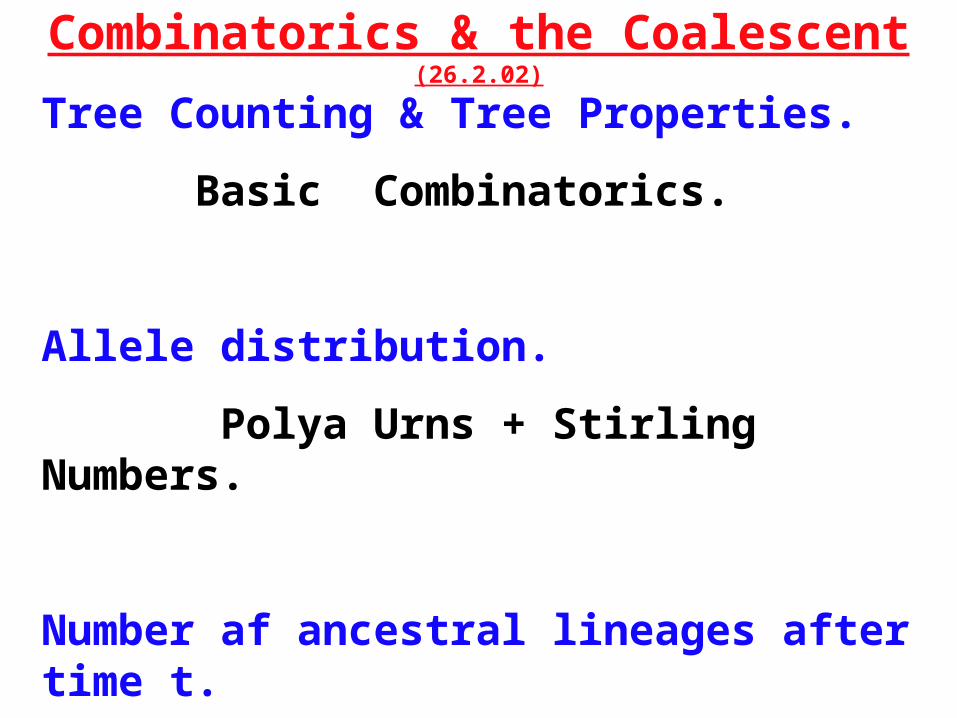
A set of realisations(from Felsenstein)

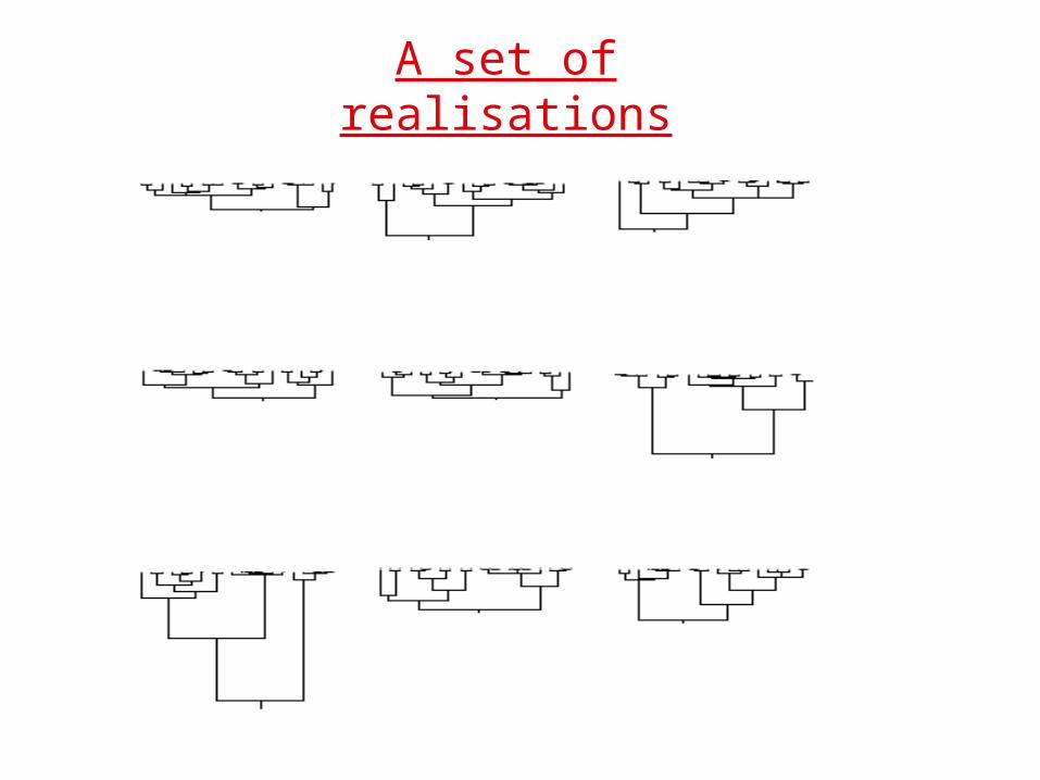
Binomial Numbers

1 2 3 4 5 n

n

r

n!

r!(n r)!n!

r!b!

1

25 34

n

Binomial Expansion:

a b n a

b

*a

b

*....*

a

b

n

i

i0

n

a ibn i

Special Cases:

11 n n

i

i0

n

2n

1 1 n n

i

i0

n

( 1) i 0

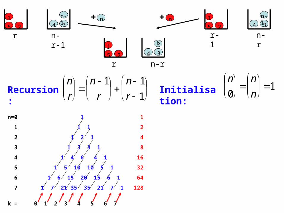
n

r

n 1

r

n 1

r 1

Recursion: Initialisation:

n

0

n

n

1

n=0 1 1

1 1 1 2

2 1 2 1 4

3 1 3 3 1 8

4 1 4 6 4 1 16

5 1 5 10 10 5 1 32

6 1 6 15 20 15 6 1 64

7 1 7 21 35 35 21 7 1 128

k = 0 1 2 3 4 5 6 7

1

25

r

34

n-1

n-r-1

34

n-1

n-r

1

25

r-11

25

r

34

6

n-r

nn+ +

0 1 2 3

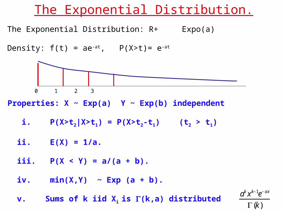
The Exponential Distribution.The Exponential Distribution: R+ Expo(a)

Density: f(t) = ae-at, P(X>t)= e-at

Properties: X ~ Exp(a) Y ~ Exp(b) independent

i. P(X>t2|X>t1) = P(X>t2-t1) (t2 > t1)

ii. E(X) = 1/a.

iii. P(X < Y) = a/(a + b).

iv. min(X,Y) ~ Exp (a + b).

v. Sums of k iid Xi is (k,a) distributed

ak xk 1e ax

(k)

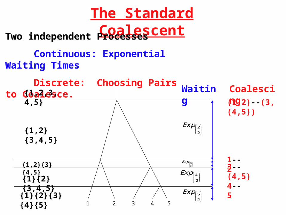
The Standard Coalescent

Two independent Processes

Continuous: Exponential Waiting Times

Discrete: Choosing Pairs to Coalesce.

1 2 3 4 5

Waiting Coalescing

4--5

3--(4,5)

(1,2)--(3,(4,5))

1--2

Exp 5

2

Exp 4

2

Exp 2

2

Exp 3

2

{1}{2}{3}{4}{5}

{1,2}{3,4,5}

{1,2,3,4,5}

{1,2}{3}{4,5}

{1}{2}{3,4,5}

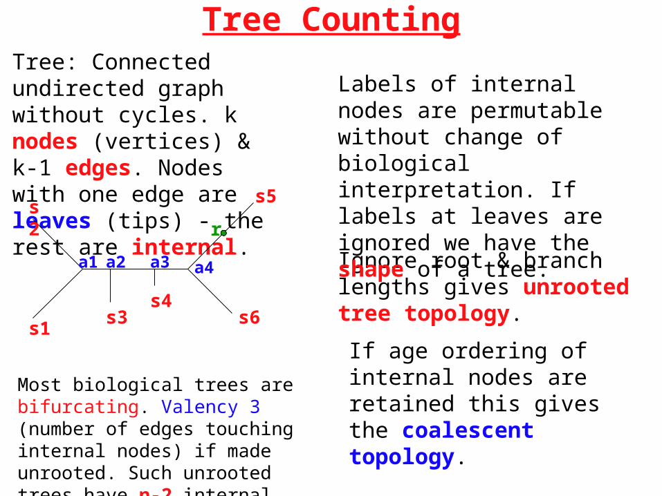
Tree CountingTree: Connected undirected graph without cycles. k nodes (vertices) & k-1 edges. Nodes with one edge are leaves (tips) - the rest are internal.

s1

s4s6

s5

s3

s2

a2a1 a3 a4

r

Ignore root & branch lengths gives unrooted tree topology.

If age ordering of internal nodes are retained this gives the coalescent topology.

Labels of internal nodes are permutable without change of biological interpretation. If labels at leaves are ignored we have the shape of a tree.

Most biological trees are bifurcating. Valency 3 (number of edges touching internal nodes) if made unrooted. Such unrooted trees have n-2 internal nodes & 2n-3 edges.

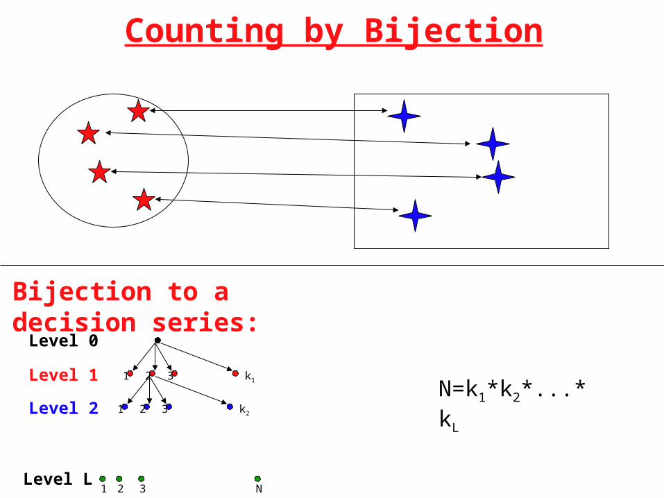
Counting by Bijection

Bijection to a decision series:

321 k1

Level 0

Level 1

Level 2

Level L

321 k2

1 32 N

N=k1*k2*...*kL

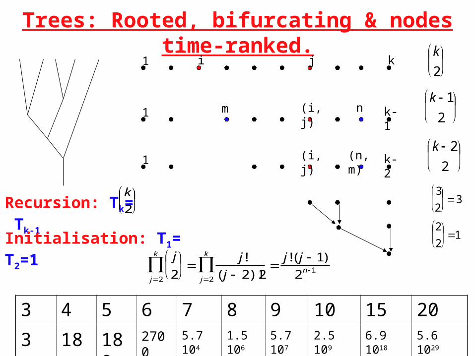
Trees: Rooted, bifurcating & nodes time-ranked.

j

2

j2

k

j!

( j 2)!2j2

k

j!( j 1)!

2n1

k1 ji

k-11 (i,j)

k

2

k 1

2

k-21 (i,j) (n,m)

m n

k 2

2

3

2

3

2

2

1

3 4 5 6 7 8 9 10 15 20

3 18 180 2700 5.7 104 1.5 106 5.7 107 2.5 109 6.9 1018 5.6 1029

Recursion: Tk= Tk-1

Initialisation: T1= T2=1

k

2

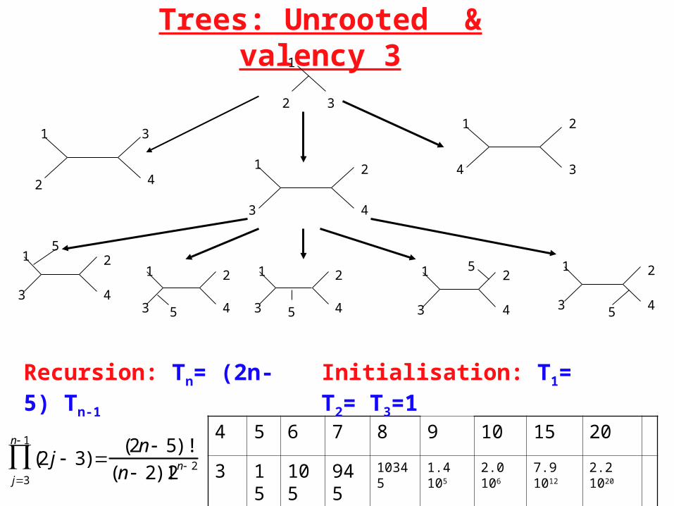
Trees: Unrooted & valency 3

2

1

3

11

24

23

31 2

3 4

4

1 2

3 4

1 2

3 4

1 2

3 4

1 2

3 4

1 2

3 4

5

5 5

5

5

(2 j 3)j3

n 1

(2n 5)!

(n 2)!2n 2

4 5 6 7 8 9 10 15 20

3 15 105 945 10345 1.4 105 2.0 106 7.9 1012 2.2 1020

Recursion: Tn= (2n-5) Tn-1 Initialisation: T1= T2= T3=1

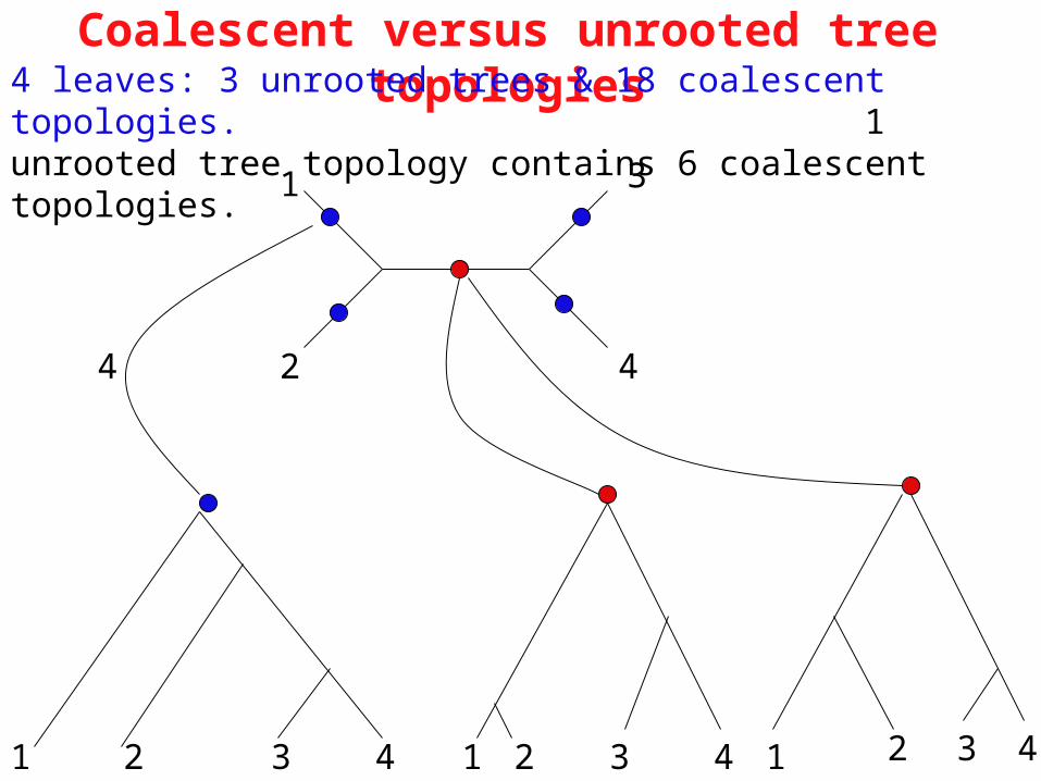
Coalescent versus unrooted tree topologies4 leaves: 3 unrooted trees & 18 coalescent topologies. 1 unrooted tree topology contains 6 coalescent topologies.

1

42

3

4

11 1 222 3 3 3 444

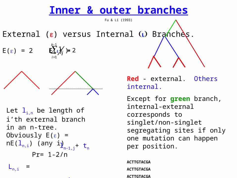
External () versus Internal Branches.

E() = 2 E() =

Inner & outer branchesFu & Li (1993)

( 1i

i1

k 1

) 2

Red - external. Others internal.

Except for green branch, internal-external corresponds to singlet/non-singlet segregating sites if only one mutation can happen per position.

ACTTGTACGA

ACTTGTACGA

ACTTGTACGA

TCTTATACGA

ACTTATACGA

s n

Let li,n be length of i’th external branch in an n-tree. Obviously E() = nE(ln,i) (any i)

ln-1,j+ tn Pr= 1-2/n

Ln,i =

tn Pr= 2/n

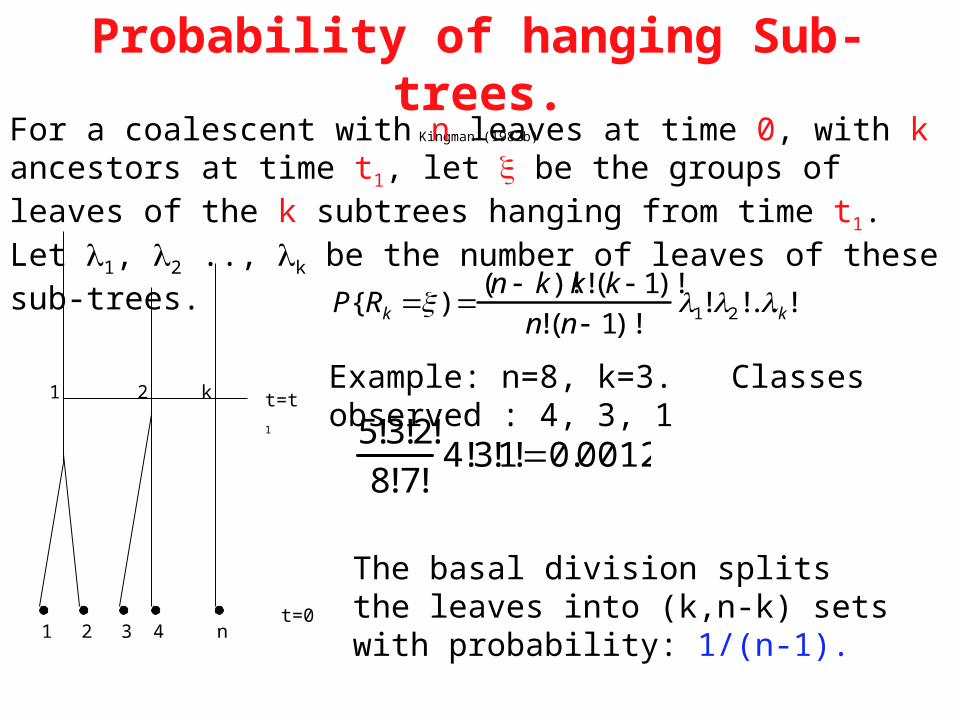
Probability of hanging Sub-trees.Kingman (1982b)

P{Rk ) (n k)!k!(k 1)!

n!(n 1)!1!2!..k!

1 2 43 nt=0

t=t11 2 k

For a coalescent with n leaves at time 0, with k ancestors at time t1, let be the groups of leaves of the k subtrees hanging from time t1. Let 1, 2 .., k be the number of leaves of these sub-trees.

Example: n=8, k=3. Classes observed : 4, 3, 1

5!3!2!

8!7!4!3!1!0.0012

The basal division splits the leaves into (k,n-k) sets with probability: 1/(n-1).

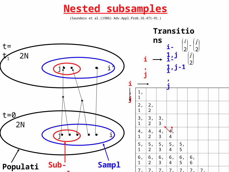
Nested subsamples(Saunders et al.(1986) Adv.Appl.Prob.16.471-91.)

t=0

Population Sub-sample Sample

t=t1

i’

ij

j’

2N

2N

Transitions

i,j

i-1,j

i-1,j-1

i,j

1,1

2,1 2,2

3,1 3,2 3,3

4,1 4,2 4,3 4,4

5,1 5,2 5,3 5,4 5,5

6,1 6,2 6,3 6,4 6,5 6,6

7,1 7,2 7,3 7,4 7,5 7,6 7,7

8,1 8,2 8,3 8,4 8,5 8,6 8,7 8,8

9,1 9,2 9,3 9,4 9,5 9,6 9,7 9,8 9,9

i , j

i

2

j

2

j

2

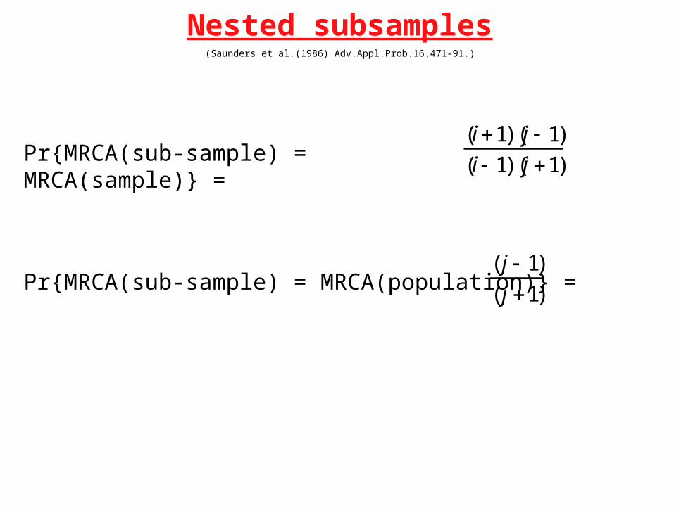
Nested subsamples(Saunders et al.(1986) Adv.Appl.Prob.16.471-91.)

Pr{MRCA(sub-sample) = MRCA(sample)} =

(i1)( j 1)

(i 1)( j 1)

Pr{MRCA(sub-sample) = MRCA(population)} =

( j 1)

( j 1)

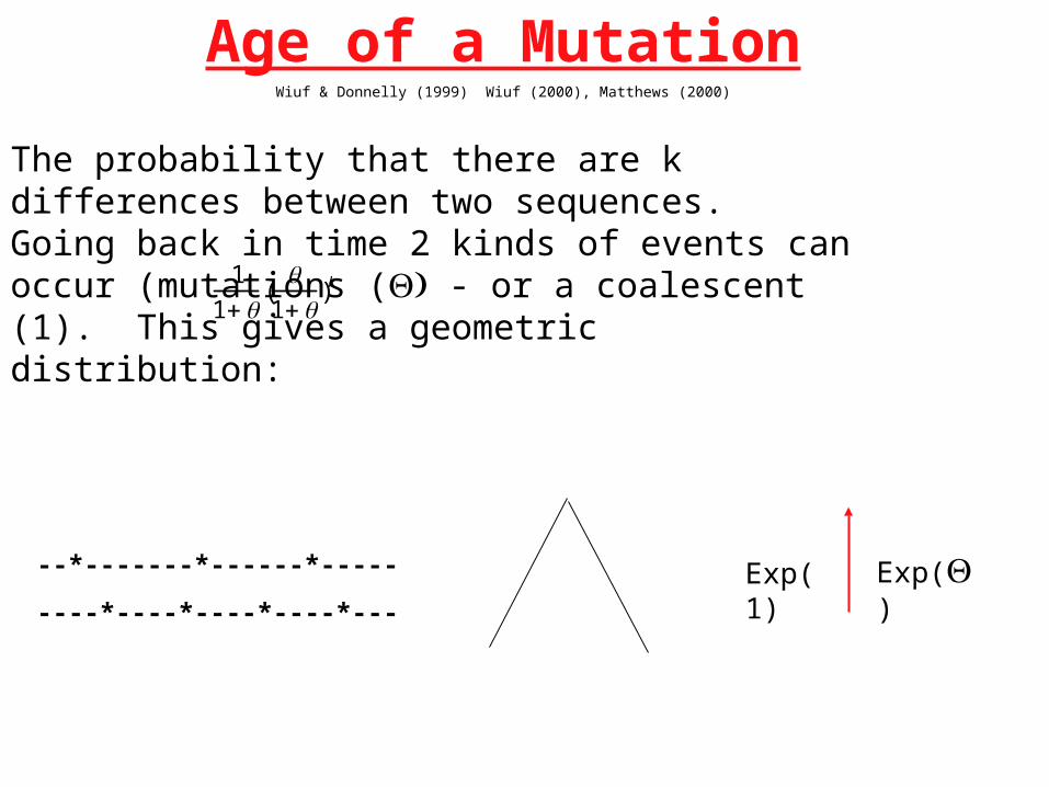
Age of a MutationWiuf & Donnelly (1999) Wiuf (2000), Matthews (2000)

The probability that there are k differences between two sequences. Going back in time 2 kinds of events can occur (mutations ( - or a coalescent (1). This gives a geometric distribution:

1

1 (

1

)k

--*-------*------*-----

----*----*----*----*---Exp(1) Exp()

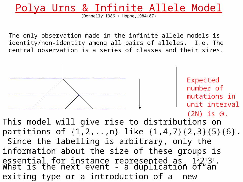
Polya Urns & Infinite Allele Model(Donnelly,1986 + Hoppe,1984+87)

The only observation made in the infinite allele models is identity/non-identity among all pairs of alleles. I.e. The central observation is a series of classes and their sizes.

What is the next event - a duplication of an exiting type or a introduction of a ”new” allele.

This model will give rise to distributions on partitions of {1,2,..,n} like {1,4,7}{2,3}{5}{6}. Since the labelling is arbitrary, only the information about the size of these groups is essential for instance represented as 122131.

Expected number of mutations in unit

interval (2N) is .

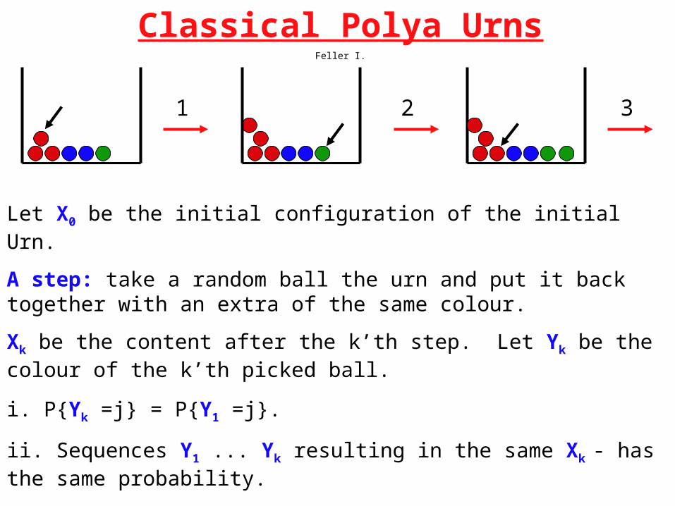
Classical Polya UrnsFeller I.

21 3

Let X0 be the initial configuration of the initial Urn.

A step: take a random ball the urn and put it back together with an extra of the same colour.

Xk be the content after the k’th step. Let Yk be the colour of the k’th picked ball.

i. P{Yk =j} = P{Y1 =j}.

ii. Sequences Y1 ... Yk resulting in the same Xk - has the same probability.

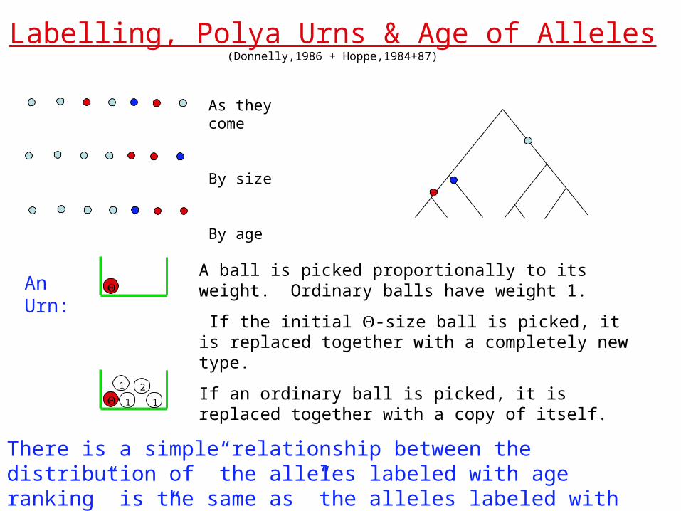
Labelling, Polya Urns & Age of Alleles(Donnelly,1986 + Hoppe,1984+87)

An Urn:

1

2

1

1

A ball is picked proportionally to its weight. Ordinary balls have weight 1.

If the initial -size ball is picked, it is replaced together with a completely new type.

If an ordinary ball is picked, it is replaced together with a copy of itself.

There is a simple relationship between the distribution of ”the alleles labeled with age ranking” is the same as ”the alleles labeled with size ranking”

As they come

By size

By age

n!

(1)..( n 1)(

a j

ja j a j!)

j1

n

j 1j1

n

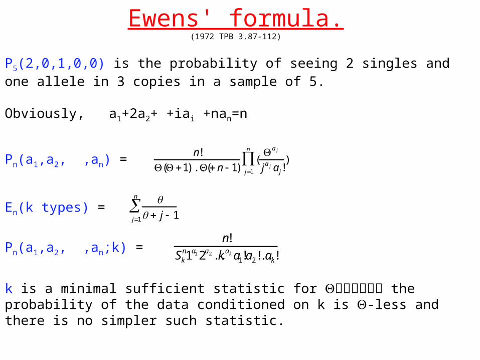
Ewens' formula.(1972 TPB 3.87-112)

n!

Skn1a1 2a2 ..k aka1!a2!..ak!

Pn(a1,a2, ,an) =

k is a minimal sufficient statistic for the probability of the data conditioned on k is -less and there is no simpler such statistic.

Pn(a1,a2, ,an;k) =

En(k types) =

P5(2,0,1,0,0) is the probability of seeing 2 singles and one allele in 3 copies in a sample of 5.

Obviously, a1+2a2+ +iai +nan=n

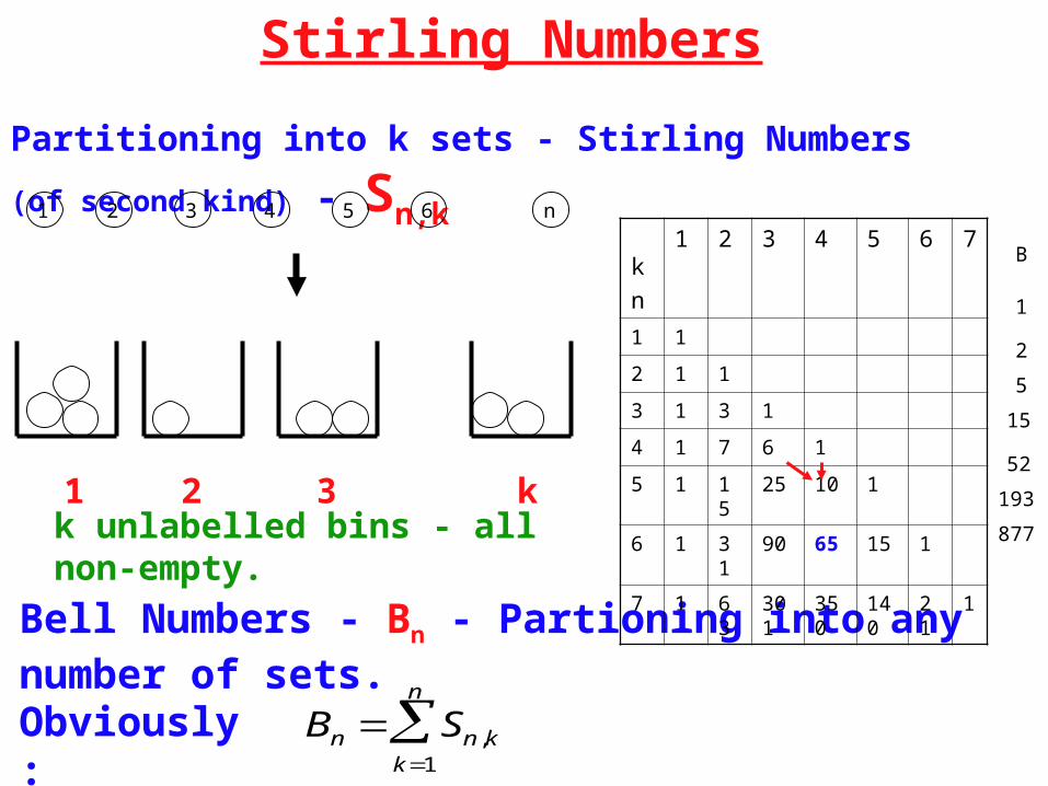
Stirling Numbers

Partitioning into k sets - Stirling Numbers (of second kind) - Sn,k

k unlabelled bins - all non-empty.

Bell Numbers - Bn - Partioning into any number of sets.

k

n

1 2 3 4 5 6 7

1 1

2 1 1

3 1 3 1

4 1 7 6 1

5 1 15 25 10 1

6 1 31 90 65 15 1

7 1 63 301 350 140 21 1

1 2 3 n5 64

1 2 3 k

Bn Sn,kk1

n

Obviously:

B

1

2

5

15

52

193

877

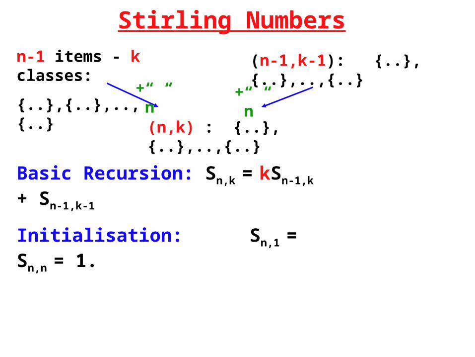
Stirling Numbers

Basic Recursion: Sn,k = kSn-1,k + Sn-1,k-1

Initialisation: Sn,1 = Sn,n = 1.

n-1 items - k classes:

{..},{..},..,{..}

(n-1,k-1): {..},{..},..,{..}

(n,k) : {..},{..},..,{..}

+ ”n” + ”n”

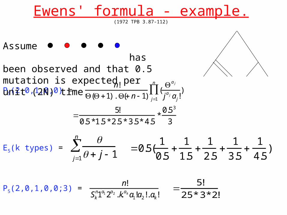
Ewens' formula - example.(1972 TPB 3.87-112)

n!

(1)..( n 1)(

a j

ja j a j!)

j1

n

P5(2,0,1,0,0) =

n!

Skn1a1 2a2 ..k aka1!a2!..ak!

P5(2,0,1,0,0;3) =

Assume has been observed and that 0.5 mutation is expected per unit (2N) time.

j 1j1

n

E5(k types) =

0.5(1

0.5

1

1.5

1

2.5

1

3.5

1

4.5)

5!

0.5 *1.5 *2.5 * 3.5* 4.5*

0.53

3

5!

25 * 3*2!

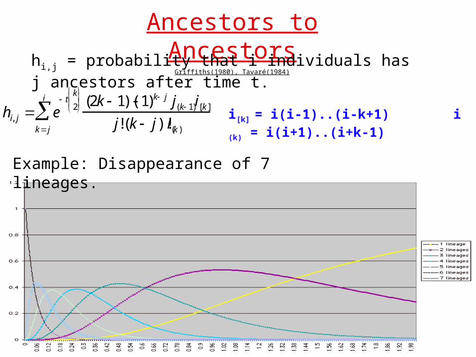
Ancestors to AncestorsGriffiths(1980), Tavaré(1984)

hi,j = probability that i individuals has j ancestors after time t.

hi, j e t

k

2

kj

i

(2k 1)( 1) k j j(k 1)i[k ]

j!(k j)!i(k )

i[k] = i(i-1)..(i-k+1) i (k) = i(i+1)..(i+k-1)

Example: Disappearance of 7 lineages.

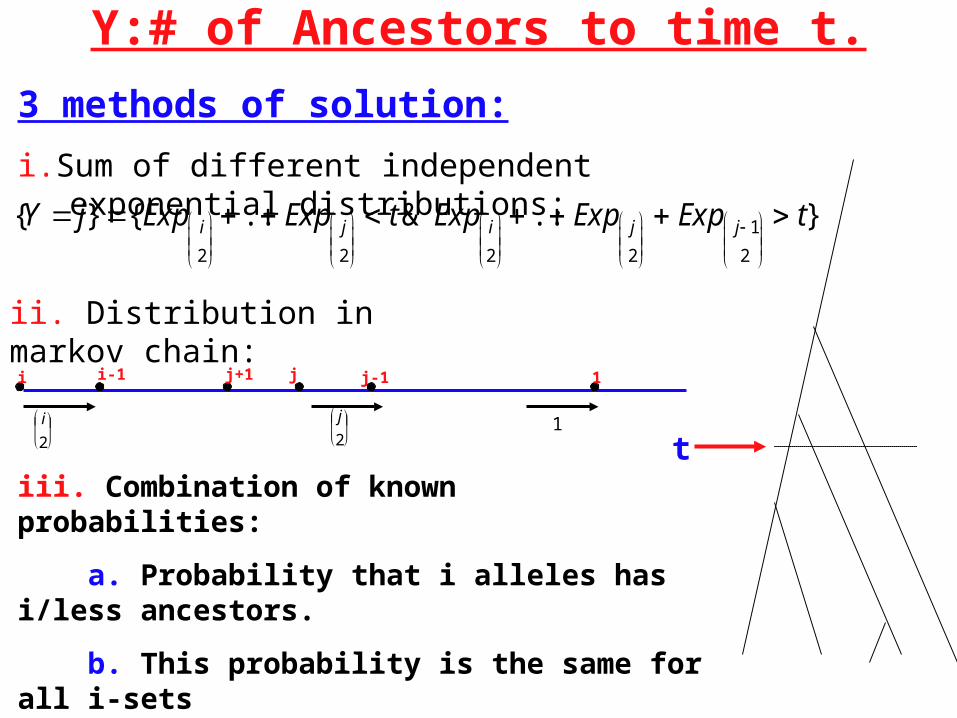
Y:# of Ancestors to time t.

3 methods of solution:

i.Sum of different independent exponential distributions:

ii. Distribution in markov chain:

iii. Combination of known probabilities:

a. Probability that i alleles has i/less ancestors.

b. This probability is the same for all i-sets

c. No coalescence within a set, implies no

coalescence within all subsets.

{Y j} {Exp i

2

.. Exp j

2

t& Exp i

2

.. Exp j

2

Exp j 1

2

t}

i j-1 1i-1 j+1 j

i

2

j

2

1

t

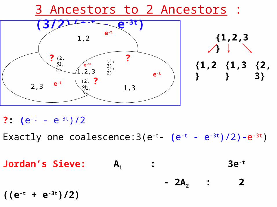
3 Ancestors to 2 Ancestors : (3/2)(e-t - e-3t)

?: (e-t - e-3t)/2

Exactly one coalescence:3(e-t- (e-t - e-3t)/2)-e-3t)

1,2

2,3 1,3

1,2,3

(2,3)

(1,2)

(1,3)

e-3t

e-t

(2,3)

(1,3)(1,2)

e-t

e-t ?

? ?

{1,2,3}

{1,2} {1,3} {2,3}

Jordan’s Sieve: A1 : 3e-t

- 2A2 : 2 ((e-t + e-3t)/2)

+ 3A3 : 3 e-3t

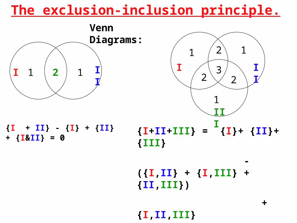
The exclusion-inclusion principle.

1 12I II

Venn Diagrams:

{I + II} - {I} + {II} + {I&II} = 0

11

1

2

2 23

III

III

{I+II+III} = {I}+ {II}+ {III}

- ({I,II} + {I,III} + {II,III})

+{I,II,III}

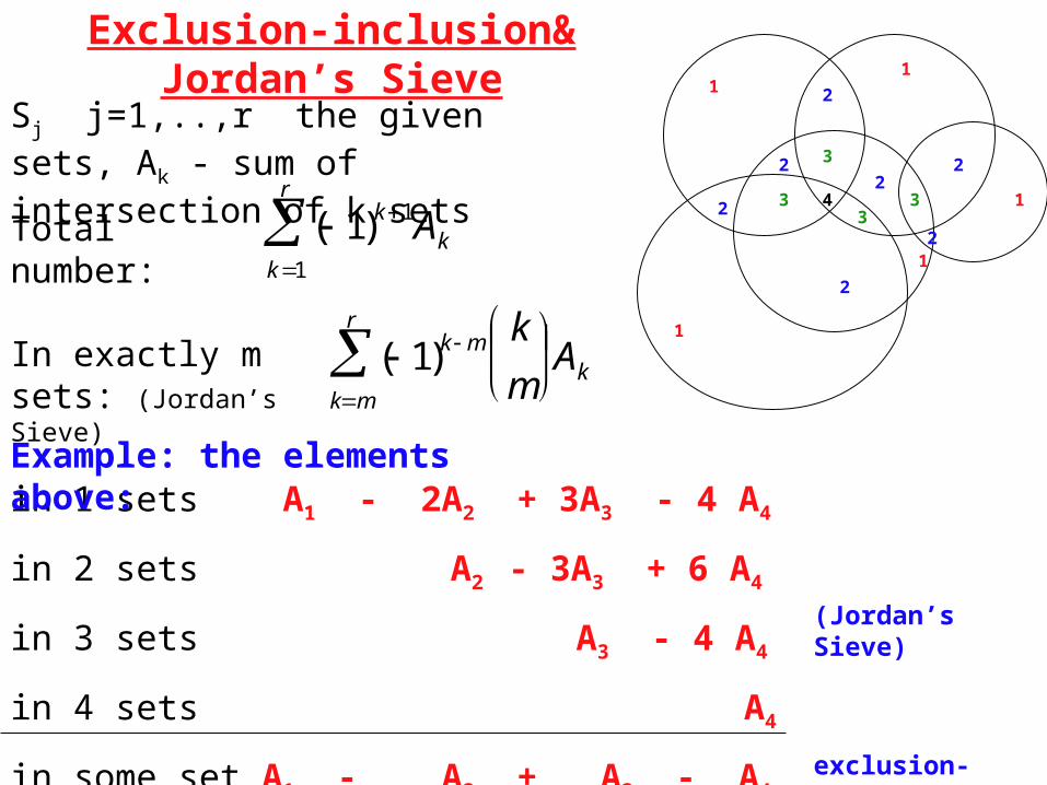
Exclusion-inclusion& Jordan’s Sieve1

1

1

1

1

2

2

2 2

2

42

3

3

3 3

2

Sj j=1,..,r the given sets, Ak - sum of intersection of k sets

( 1)k1

k1

r

Ak

in 1 sets A1 - 2A2 + 3A3 - 4 A4

in 2 sets A2 - 3A3 + 6 A4

in 3 sets A3 - 4 A4

in 4 sets A4

in some set A1 - A2 + A3 - A4

Example: the elements above:

Total number:

( 1)k m

km

r

k

m

AkIn exactly m sets:

(Jordan’s Sieve)

(Jordan’s Sieve)

exclusion-inclusion

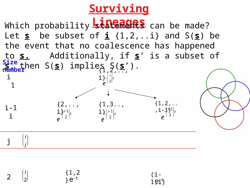
Surviving Lineages

Which probability statements can be made? Let s be subset of i {1,2,..i} and S(s) be the event that no coalescence has happened to s. Additionally, if s’ is a subset of s, then S(s) implies S(s’).

{2,..,i} {1,2,..,i-1}

ei1

2

t

{1,3..,i}

ei1

2

t

{1,2,..,i}

ei

2

ti 1

i-1 i

Size number

{1,2}e-t

(i-1,i)e-t2

i

2

i

j

j

ei1

2

t

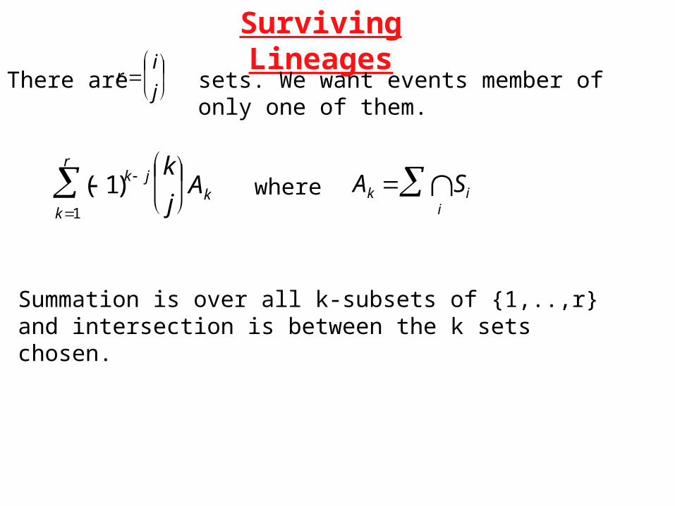
Surviving Lineages

( 1)k j

k1

r

k

j

Ak where

ri

j

There are sets. We want events member of only one of them.

Ak Sii

Summation is over all k-subsets of {1,..,r} and intersection is between the k sets chosen.

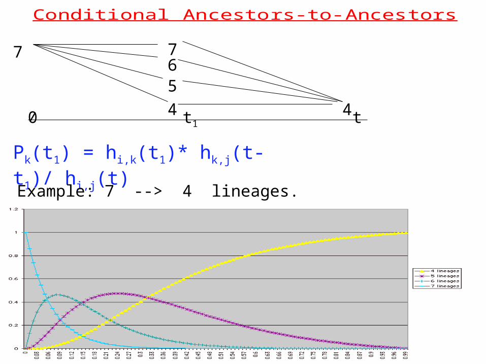
Conditi onal Ancesto r s-to- Ancest ors

0 t1 t

77

4

56

4

Pk(t1) = hi,k(t1)* hk,j(t- t1)/ hi,j(t)

Example: 7 --> 4 lineages.

Summary

Tree Counting & Tree Properties.

Basic Combinatorics.

Allele distribution.

Polya Urns + Stirling Numbers.

Number af ancestral lineages after time t.

Inclusion-Exclusion Principle.

Recommended LiteratureBender(1974) Asymmptotic Methods in Enumeraion Siam Review vol16.4.485-

Donnelly (1986) ”Theor.Pop.Biol.

Ewens (1972) Theor.Pop.Biol.

Ewens (1989) ”Population Genetics Theory - The Past and the Future”

Feller (1968+71) Probability Theory and its Applications I + II Wiley

Fu & Li (1993) ”Statistical Tests of Neutrality of Mutations” Genetics 133.693-709.

Griffiths (1980)

Griffiths & Tavaré(1998) ”The Age of a mutation on a general coalescent tree.

Griffiths & Tavaré(1999) ”The ages of mutations in gene trees”

Griffiths & Tavaré(2001) ”The genealogy of a neutral mutation”

Hoppe (1984) ”Polya-like urns and the Ewens’ sampling formula” J.Math.Biol. 20.91-94

Kingman (1982) ”On the Genealogy of Large Populations” 27-43.

Kingman (1982) ”The Coalescent” Stochastic Processes and their Applications 13..235-248.

Kingman (1982)

Matthews,S.(1999) ”Times on Trees, and the Age of an Allele” Theor.Pop.Biol. 58.61-75.

Möhle

Pitman

Schweinsberg

Simonsen & Churchill (1997)

Saunders et al.(1986) ”On the genealogy of nested subsamples from a haploid population” Adv.Apll.Prob. 16.471-91.

Tajima (1983) Evolutionary Relationships of DNA Sequences in Finite Poulations Genetics 105.437-60.

Tavaré (1984) Line-of-Descent and Genealogical Processes, and Their Application in Population Genetics Models. Theor.Pop.Biol. 26.119-164.

Thompson,R. (1998) ”Ages of mutations on a coalescent tree” Math.Bios. 153.41-61.

van Lint & Wilson (1991) A Course in Combinatorics - Cambridge

Wiuf (2000) On the Genealogy of a Sample of Neutral Rare Alleles. Theor.Pop.Biol. 58.61-75.

Wiuf & Donnelly (1999) Conditional Genealogies and the Age of a Mutant. Theor. Pop.Biol. 56.183-201.