Comet Shoemaker–Levy 9 Dust Size and Velocity Distributions

Joseph M. Hahn

Lunar and Planetary Institute, 3600 Bay Area Boulevard, Houston, TX 77058email: hahn@lpi.usra.edu

phone: 281–486–2113fax: 281–486–2162

Terrence W. Rettig

Department of Physics, University of Notre Dame, Notre Dame, IN 46556email: trettig@nd.eduphone: 219–631–7732fax: 219–631–5952

To appear in Icarus

– 2 –

ABSTRACT

Pre–impact observations of Comet Shoemaker–Levy 9 obtained with the Hubble Space Tele-scope are examined, and a model of an active, dust–producing comet is fitted to images of fragmentsG, H, K, and L. The model assumes steady isotropic dust emission from each fragment’s sunlit hemi-sphere. Best–fit results indicate that the dominant light–scatterers in these fragments’ comae wererelatively large dust grains of radii 10 µm . R . 3 mm. The fragments’ dust size distributionswere rather flat in comparison to other comets, dN(R) ∝ R−2.3±0.1, and the dust ejection speedswere ∼ 0.5–1.5 m/sec. The S–L 9 fragments themselves were not detected directly, and upper limitson their radii are 1.0–1.5 km assuming an albedo a = 0.04. However these fragments’ vigorous pro-duction of dust, which ranges from 6–22 kg/sec, places a lower limit of ∼ 100 meters on their radiiat the moment of tidal breakup. Any fragments smaller than this limit yet experiencing similarmass loss rates would have dissipated prior to impact. Such bodies would fail to leave an impactscar at Jupiter’s atmosphere, as was realized by fragments F, J, P1, P2, T, and U.

– 3 –

1. Introduction

Owing to an extremely close encounter with Jupiter on July 7, 1992, Comet Shoemaker–Levy9 (S–L 9) tidally disrupted into approximately 21 cometary fragments. Tidal disruption effectivelyturned S–L 9 “inside out”, which permitted a rare examination of the interior of a comet. Of course,comet observations generally provide information only about its smallest constituents, namely, thedust grains and gas molecules that manage to escape from a nucleus that usually remains hiddenfrom view due to the surrounding coma. Although this study is no exception to this difficulty, weshall nonetheless manage to draw some conclusions about the tidally disrupted S–L 9 fragmentsvia a close examination of their dusty comae. In particular, a model of a cometary dust coma andtail is fitted to Hubble Space Telescope (HST) observations of S–L 9 in order to extract the comet’sdust size and velocity distributions, as well as to place constraints on the size of the fragmentsthemselves.

Although Comet S–L 9 was monitored regularly since its discovery in March 1993, we shall ex-amine only the highest resolution observations that were acquired between January 1994 (whenthe comet was not far from apojove) and July 1994, just prior to impact with Jupiter (see(Weaver et al. 1995)). This analysis shall concentrate on the five bright fragments G, H, K, L,and S that were observed on several occasions when both far from and near to Jupiter. Relevantparameters for these observations are given in Table I. Comet S–L 9 was imaged with the HSTWide Field Planetary Camera 2 using the F702W filter, which is roughly and R filter having abandpass of 6000 to 8100 A. Comet S–L 9 was observed at a geocentric distance of about 5 AU,so each 0.1′′ pixel in the Wide Field Camera subtends about 400 km. Exposures typically lastedabout 30 minutes. The data were reduced in the standard manner, with the bias and dark currentssubtracted, the images flatfielded and background subtracted, and cosmic ray hits repaired. Forfurther details see (Hahn et al. 1996).

Spectroscopic observations of S–L 9 did not detect any signatures of cometary gas emissions((Cochran et al. 1994), (Weaver et al. 1995)). Nonetheless, the inferred upper limit for water pro-duction is consistent with non–rotating comet fragments that are smaller than about 15 km across((Weissman 1996)). Although direct evidence for any gas production is absent, the emission of dustentrained by an unseen gas outflow is the most promising explanation for the Comet’s appearance1.Thus a simple model of an active, dust producing comet is investigated in Section 2. Syntheticdust–coma images are generated in Section 3 and fitted to the HST observations of S–L 9. Section4 reports results for the S–L 9 dust size and velocity distributions and also places constraints on

1Note that the early S–L 9 literature assumed that the Comet was largely inactive, and that each frag-

ment’s dust halo was instead composed of large dust created during the tidal breakup event ((Weaver et al. 1994),

(Sekanina et al. 1994)). However this scenario cannot account for the observed coma–morphology since an initial dust

halo would have subsequently evolved into an elongated structure having isophotes that would steadily lengthen and

narrow along over time, concurrent with the growing separations among the fragments themselves ((Weissman 1996),

(Rettig and Hahn 1997), (Tanigawa et al. 1997)).

– 4 –

the fragment sizes. Section 5 then synthesizes our findings for this tidally disrupted comet.

2. The Dust Coma/Tail Model

The task at hand is to determine the rates at which a given S–L 9 fragment produced dustgrains of various radii R as well as their ejection velocities V (R). We begin by defining N(R, t) asthe cumulative number of all dust grains having radii smaller than R emitted up until some timet. The differential dust production rate of all grains within the size interval R± dR/2 is written as

d

dt

dN(R, t)dR

× dR, (1)

or more simply dN(R, t), which is one of the quantities to be extracted from the HST observations.However it is usually quite difficult to uniquely disentangle the dust size distribution dN(R, t) fromthe dust emission velocity distribution V (R, t) without first making some simplifying assumptions.

The standard approach is to assume that the dust size and velocity distributions obey simplepower–laws which then permits their characterization in terms of a few parameters that might varywith time. However S–L 9 maintained a nearly constant distance from the Sun (Table I), and whenfar from Jupiter all the fragments considered here exhibited surface brightness profiles consistentwith steady dust production ((Hahn et al. 1996), (Rettig and Hahn 1997)). This suggests thatthese fragments’ dust production rates did not vary dramatically during the observation spanconsidered here. For these reasons the remainder of this analysis assumes the dust size distributiondN(R) and outflow velocity distribution V (R) were constant over time. This makes any a prioripower–law assumptions unnecessary. But in order to make the problem computationally tractable,the model comet shall only emit dust having discrete radii Ri = 0.316 µm, 1.0 µm, ..., 3.16 mm, 1cm (i.e., with sizes incrementing every half-decade) rather than a continuous range of dust sizes.This analysis thus seeks the approximate S–L 9 dust distribution dN (Ri) and velocity distributionV (Ri) evaluated at ten discrete size bins. The permitted dust ejection velocities are similarlydiscrete over 0.25 m/sec intervals, with velocities ranging from 0 up to 3.5 m/sec in fifteen velocitybins. The dust size and velocity bins considered here are chosen to span the range of sizes andvelocities reported previously ((Hahn et al. 1996), (Rettig et al. 1996)), and the number of binsused here reflects a reasonable balance between the model’s precision and the cost in CPU time,which increases geometrically with the number of bins.

The model comet nucleus and its dust grains are subject to solar and jovian gravities, withthe dust also perturbed by solar radiation pressure. The bulk of the S–L 9 dust were evidentlylarger that the wavelength of visible light ((Hahn et al. 1996)), so the ratio of radiation pres-sure to the solar acceleration is simply β = 3L�Qr/16πGM�cρdR in the geometric optics limit((Burns et al. 1979)), where L� is the solar luminosity, Qr is the radiation pressure efficiency,c the speed of light, ρd the grain density, and R the grain radius. Cometary dust as well asthe surfaces of nuclei are very dark and efficient absorbers of light ((Hanner and Newburn 1989),

– 5 –

(Weissman et al. 1989)), so setting Qr = 1 is a good approximation. For simplicity this analysisshall assume that the unknown density of the S–L 9 dust is ρd = 1 gm/cm3; if an alternate densityis preferred then the grain sizes quoted herein should be rescaled by by a factor of ρ−1

d . Thusβ ' 0.585(R/1 µm)−1 provided R exceeds about 1 µm. For grains smaller than R = 1 µm weadopt a value for β computed via Mie light-scattering theory for an “ideal” grain that absorbsonly the incident sunlight that is of a wavelength shorter than the grain diameter (see Fig. (7b) of(Burns et al. 1979) and adjust for the ρd = 1 gm/cm3 grain density employed here).

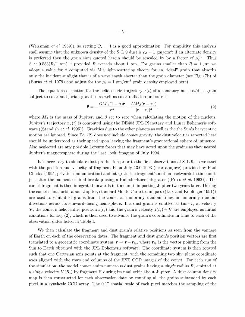
The equations of motion for the heliocentric trajectory r(t) of a cometary nucleus/dust grainsubject to solar and jovian gravities as well as solar radiation pressure is

r = −GM�(1 − β)rr3

− GMJ (r− rJ)|r− rJ |3 , (2)

where MJ is the mass of Jupiter, and β set to zero when calculating the motion of the nucleus.Jupiter’s trajectory rJ(t) is computed using the DE403 JPL Planetary and Lunar Ephemeris soft-ware ((Standish et al. 1995)). Gravities due to the other planets as well as the the Sun’s barycentricmotion are ignored. Since Eq. (2) does not include comet gravity, the dust velocities reported hereshould be understood as their speed upon leaving the fragment’s gravitational sphere of influence.Also neglected are any possible Lorentz forces that may have acted upon the grains as they nearedJupiter’s magnetosphere during the ‘last–look’ imaging of July 1994.

It is necessary to simulate dust production prior to the first observations of S–L 9, so we startwith the position and velocity of fragment H on July 13.0 1993 (near apojove) provided by PaulChodas (1995, private communication) and integrate the fragment’s motion backwards in time untiljust after the moment of tidal breakup using a Bulirsh–Stoer integrator ((Press et al. 1992)). Thecomet fragment is then integrated forwards in time until impacting Jupiter two years later. Duringthe comet’s final orbit about Jupiter, standard Monte Carlo techniques ((Lux and Koblinger 1991))are used to emit dust grains from the comet at uniformly random times in uniformly randomdirections across its sunward–facing hemisphere. If a dust grain is emitted at time te at velocityV, the comet’s heliocentric position r(te) and the grain’s velocity r(te) +V are employed as initialconditions for Eq. (2), which is then used to advance the grain’s coordinates in time to each of theobservation dates listed in Table I.

We then calculate the fragment and dust grain’s relative positions as seen from the vantageof Earth on each of the observation dates. The fragment and dust grain’s position vectors are firsttranslated to a geocentric coordinate system, r → r− r⊕, where r⊕ is the vector pointing from theSun to Earth obtained with the JPL Ephemeris software. The coordinate system is then rotatedsuch that one Cartesian axis points at the fragment, with the remaining two sky–plane coordinateaxes aligned with the rows and columns of the HST CCD images of the comet. For each run ofthe simulation, the model comet emits numerous dust grains having a single radius Ri emitted ata single velocity V (Ri) by fragment H during its final orbit about Jupiter. A dust column densitymap is then constructed for each observation date by counting all the grains subtended by eachpixel in a synthetic CCD array. The 0.1′′ spatial scale of each pixel matches the sampling of the

– 6 –

detector in the Wide–Field camera, and the resulting synthetic images are centered on the S–L9 fragment and measure 20′′ across. (There is little need to model the dust tails beyond about10′′ of the comae photocenters since the tails’ signal/noise ratios have dropped to ∼ 1 beyond thisdistance.) The production of ∼ 106 grains over the comet’s two-year orbit was more than sufficientto generate Monte Carlo dust tail models having statistical fluctuations much smaller than wasobserved in the S–L 9 data. In Section 3, the contributions by grains of various sizes Ri and speedsV (Ri) will be coadded in order to assemble a more realistic image of a cometary dust coma andtail.

Computation of the five images requires about ten hours of CPU time on an IBM RS6000,and this is repeated 150 times—once for each of the ten dust size bins for grains emitted at thefifteen different velocities. Finally, the images are convolved with the HST point spread function(PSF) to account for light diffraction caused by the telescope’s optical system. The model PSFused here is computed with Tiny Tim, a standard software package used to generate PSFs for HSTdata ((Krist 1994)). Example model images are provided in Fig. 1 which shows contour maps foran Ri = 300 µm, V (Ri) = 0.75 m/sec model on two dates. Although these images were generatedspecifically for the observations of fragment H, they will also be used to fit images of the otherfragments since they all followed the same path into Jupiter; except when imaged just prior toimpact, the observed fragments were nearly equidistant from Jupiter.

3. Dust Coma Fitting

The resulting dust column density images generated in Section 2 are divided by the model’sdust production rate so that each image now represents the column density of a comet having‘unit’ dust production rate. These column density maps shall be denoted as %(x,Ri, V (Ri), t)where x represents a particular pixel in the CCD image of dust having radii Ri emitted at velocityV (Ri) and observed at time t. The dust column density contributed by a single grain size bin is%(x,Ri, V (Ri), t) × dN(Ri), so the total flux density of sunlight reflected by the model comet issimply

F (x, t) =∫

R%(x,R, V (R), t)f(R, t)dN (R) + PSF(x)f(Rf , t) (3a)

'∑Ri

%(x,Ri, V (Ri), t)f(Ri, t)dN (Ri) + PSF(x)f(Rf , t), (3b)

where f(R, t) is the flux density of sunlight reflected by a grain of radius R, and the sum is overall the grain size bins. The comet nucleus itself will also reflect sunlight, so the term on the rightrepresents the light contributed by an S–L 9 fragment of radius Rf . Here, PSF(x) is the normalizedPSF centered at the origin which accounts for how the light from an unresolved point source (thefragment) is distributed at the image plane.

The flux density of sunlight (here, power per area per wavelength interval) reflected by a

– 7 –

spherical grain of radius R toward an observer a distance ∆(t) away is ((Lester et al. 1979))

f(R, t) =(

R

∆(t)

)2

aψ(φ)finc (4)

where a is the grain’s geometric albedo, ψ(φ) is its phase law, and finc is the incident monochromaticsolar flux density. The S–L 9 dust albedo cannot be determined from these observations, so thevalue a = 0.04 measured for comet Halley ((Lorenzetti et al. 1987)) shall be adopted here. It shouldbe noted that comet dust albedos generally range from 0.02 to 0.1 ((Hanner and Newburn 1989)).Cometary dust generally obey the empirical phase law ((Meech and Jewitt 1987))

ψ(φ) = 10−β|φ(t)|/2.5 (5)

where φ(t) is the Sun–Comet–Earth phase angle given in Table I and the phase coefficient βdescribes how the grain’s reflectivity drops with phase angle. The incident solar flux density in Eq.(4) is finc = π(R�/r)2Bλ where R� is the radius of the Sun and Bλ ' 2.12×106 ergs/cm2/sec/A isthe monochromatic solar radiance for a T = 5780 K blackbody at the effective wavelength λ = 6913A of these broadband HST observations. The comet fragment also reflects sunlight as per Eq. (4)but it may have an albedo af and phase law ψf distinct from the dust. The albedo of cometarynuclei generally ranges from 0.02 to 0.2 ((Weissman et al. 1989), (Tokunaga et al. 1992)). TheHalley nucleus albedo, which is also af = 0.04 ((Sagdeev et al. 1986)), shall be assumed for theS–L 9 fragments. While the appropriate phase law for comet nuclei is unknown, it seems reasonableto treat the fragments as diffuse reflectors of light for which Lambert’s law of reflection applies. Inthis case ψf ' 1 for the small phase angles considered here.

Thus n = 22 parameters specify a single dust comet model: a dN (Ri), V (Ri) pair for eachof the ten dust size bins, the phase coefficient β, and the fragment radius Rf . The dust modelis adjusted to the five observations of each fragment by iteratively choosing trial solutions us-ing the downhill simplex algorithm ((Nelder and Mead 1965), (Parkinson and Hutchinson 1972),(Press et al. 1992)) which minimizes the fit’s χ2. Data pixels polluted by background stars, ad-jacent cometary comae, or an inordinate amount of spatially varying background flux are flaggedand are not considered in these fits. As with all numerical minimization routines, this method onlyprovides a solution that locally minimizes the χ2 along the search path through parameter space, sofits starting with numerous different trial solutions must be performed. Experience has shown thatrepeating the parameter search using ∼ 1000 widely distinct trial solutions is more than sufficientto determine the set of parameters that minimizes the fit’s χ2. Best fits reported in Figs. 2–10.

4. Results

The time-sequence of contour maps of fragment G are shown in Fig. 2 as well as the syntheticimages fitted to the observations. Although slight discrepancies exist between the observed and themodel isophotes at the fainter light levels, there is overall good agreement between the observations

– 8 –

and the fit. Figure 3 gives the differential dust production rate dN(R) as well as its mass lossdistribution dM(R) = 4π

3 ρdR3dN (R) obtained for fragment G, with the arrows indicating that

only upper limits on the dust production rates are obtained for the corresponding size bins. Thesefindings are typical of many comets in that production of the smallest grains are numerically favoredyet the total mass loss rate is governed by the largest grains ejected. The mass loss rate of grainsdetected in fragment G’s comae (10 µm. R . 3 mm) is M = 22 ± 5 kg/sec.

Radiation pressure segregates grains according to their size×density, and this is illustrated bythe network of syndynes and synchrones shown in Fig. 2. A syndyne is the trajectory of dust havinga specified radius R emitted at zero velocity at various times t, while synchrones trace zero–velocitydust of various radii R that are all emitted at a given time t. Dust of radius R emitted at velocityV > 0 thus inhabit a three–dimensional envelope that surrounds the appropriate syndyne. TheR < 3 µm syndynes shown in the May 18 image, which was acquired very near solar opposition,confirms our earlier findings in that this fragment did not produce detectable quantities of dustmuch smaller than about ∼ 5 µm ((Hahn et al. 1996)). Had R = 1 µm dust been abundant, theywould have produced a bright, narrow tail in the May 18 image extending about 7 arcseconds eastof the coma photocenter. The dearth of any detectable dust beyond ∼ 5 arcseconds to the eastinstead puts an upper limit of ∼ 70 gm/sec on the production rate of grains 3 µm and smaller byfragment G (see Fig. 3). This is well below the limit previously established by Sekanina (1996a)based on the S–L 9 tail orientations. Note also that only an upper limit on the production of largecm–sized grains has been determined. Whether an S–L 9 fragment could actually have launchedsuch large particles is doubtful. At S–L 9’s heliocentric distance, gas–flow models show that waterproduction is too feeble to loft grains larger than about 1 micron from the surface of a km–sizedcomet fragment ((Weissman 1996)).

However a more volatile species such as CO could very well be responsible for lofting the largedust grains seen at S–L 9. Consider comets Schwassmann–Wachmann 1 and Hale–Bopp, both ofwhich produced CO at rates ofQ ∼ 3×1028 molecules/sec while at r ∼ 6 AU ((Senay and Jewitt 1994),(Biver et al. 1996)). Both comet nuclei have similar radii, Rn ∼ 20 km ((Meech et al. 1993),(Weaver and Lamy 1997)), so their surface production is Z = Q/2πR2

n ∼ 1015 molecules/cm2/secassuming sunward emission. It is reasonable to expect even more vigorous CO production by theS–L 9 fragments due to the very recent exposure of their icy surfaces and their closer proxim-ity to the Sun. The largest grain that can be lofted by a CO outflow is obtained by equating afragment’s surface gravity to the gas drag force, which yields Rmax = 9CDmCOZv/32πGRfρpρd

where CD = 2 is the drag coefficient for free molecular flow, mCO is the mass of a CO molecule,and G is the gravitation constant ((Gombosi et al. 1986), (Hahn et al. 1996)). The gas velocity isv =

√3kT/mCO ∼ 0.4 km/sec where k is the Boltzmann constant and a blackbody temperature of

T = 170 K is adopted at the fragment’s surface. Assuming the fragment’s have radii Rf ∼ 0.3 km(see Section 4.2) and internal densities of ρf ∼ 0.6 gm/cm3 with dust densities of ρd ∼ 1 gm/cm3,the largest coma grain has a radius Rmax ∼ 3 mm. Of course the good agreement between Rmax

and the largest dust–grain detected at fragment G (see Fig. 3) is merely accidental since most of

– 9 –

the quanties adopted above are quite uncertain.

The grain size distribution for fragment G is also rather unique. The logarithmic slope of dN (R)in Fig. 3 over the 10 µm . R . 3 mm size interval indicates dN(R) ∝ R−a with a = 2.3 ± 0.1.The color of comet dust is also sensitive to the slope of the dust size distribution, and recentfits to the S–L 9 photometry favor a dust size power–law that is even shallower than a ∼ 2((Tanigawa et al. 1997)). Note however that these size distributions are considerably flatter thanthe R−3.7 power–law measured for comet Halley ((Tokunaga et al. 1992), (Waniak 1992)). Thusif Comet Shoemaker–Levy 9 had produced small grains in the same proportions as Comet Halleythen they would have been well above detection limits, as indicated by Fig. 3. It is possible thatthis overabundance of large grains in the S–L 9 comae is due to its tidally disrupted nature—sinceany ancient surface mantle is largely absent, large dust grains might escape the fragments withgreater ease.

The dust outflow velocity distribution V (R) is given in Fig. 4 for the detected 10 µm ≤ R ≤3 mm grains, and obeys a power–law relation V ∝ R−b having b = 0.3± 0.1. The observed power–law dependence is somewhat weaker than b = 0.5 predicted by the theory of dusty–gas emissionfrom cometary surfaces ((Gombosi et al. 1986)), but this finding is typical of other comet studies(e.g., (Fulle 1990), (Fulle 1992), (Fulle 1996); (Waniak 1992)). The observed velocities are also ingood agreement with earlier estimates ((Hahn et al. 1996), (Rettig et al. 1996)).

The upper limits on the production rates reported in Fig. 3 for grains R ≤ 3 µm assume a dustoutflow velocity of 3.5 m/sec. However if the small grains were ejected at a different velocity V ′,then the upper limits dN and dM for these grains should be adjusted by a factor V ′/(3.5 m/sec)since imaging can only constrain the grains’ column density which varies as dN(R)/V (R). Theupper limit on the production of R = 1 cm grains assumes an outflow velocity V ′ = 1 m/sec (thearrow in Fig. 4) and thus yields a conservative limit on the mass loss rate for these grains.

The statistical uncertainties quoted in the Figs. 3–4 represent 68% confidence intervals inthe model parameters assuming a constant dust grain density ρd = 1 gm/cm3 and a dust albedoa = 0.04. Thus the results reported here are further affected by the systematic uncertaintiesassociated with the unknown bulk density of comet dust and their albedo. Radiation pressure sortsdust grains according to the product ρdR, so if the true S–L 9 grain density ρd differs from the valueassumed here then the R axis in Figs. 3–4 should be divided by a factor ρd expressed in cgs units.The observed flux reflected by each grain size bin determines aR2dN(R), so if an alternate albedo ais also preferred, the grain production rates in Fig. 3 should be multiplied by 0.04ρ2

d/a. However ifthe grain density ρd is independent of grain size R (which might not be true if the smaller cometarygrains are fluffy instead of compact), then the mass loss rates dM (R) ∝ ρdR

3dN (R) reported inFig. 3 are independent of the assumed grain density but still uncertain by a factor of 0.04/a.

The parameter search yields a phase law coefficient β = 0.024±0.003 magnitudes/degree, whichis typical for comets that generally exhibit β = 0.01 to 0.04 mag/degree ((Meech and Jewitt 1987)).The colors of the S–L 9 comae were also similar to most other comets ((Cochran et al. 1994),

– 10 –

(Meech and Weaver 1996)), further indicating that the light scattering properties of the S–L 9 dustwere otherwise unremarkable.

Figures 5—10 show the model fits for fragments H, K, and L as well as their dust size/velocitydistributions (results for fragment K are also reported in (Rettig and Hahn 1997)). All the im-portant characteristics extracted from these fits are summarized in Table II which lists the dustmass loss rate M for the detected grains, the power–law indices a and b for the dust size/velocitydistributions, the upper limit on the fragment radius Rf, max, and the dust phase coefficient β.In general the model is able to reproduce all the features exhibited by the S–L 9 tails, such astheir westward orientation seen just after solar opposition as well as the comae elongation andenhanced brightness toward Jupiter that was observed as the fragments approached the planet.However systematic discrepancies are evident, for the simulated isophotes very often lie just inte-rior to the observed tailward isophotes. Better agreement might be achieved with a model thatconsiders anisotropic or perhaps spherical dust emission patterns rather than the hemisphericaldust emission considered here. Also recall that the dust tail model is time–independent, so thedust production rates reported here should be considered an average over the six–month span ofS–L 9 observations considered here. Better agreement between the simulations and observationsmight also be achieved with a time–dependent model of dust production.

4.1. Fragments S and T

The parameter search algorithm was unable to find a satisfactory fit to the observations offragment S, the contours of which are shown in Fig. 11. This failure is most likely a consequenceof a bilateral asymmetry evident in this fragment’s coma and tail that was first described as a“brightness spur” ((Weaver 1994a), (Weaver 1994b)). This asymmetry is revealed in Fig. 12 whichshows the ratio of the surface brightness of fragment S to the average of fragments G, H, and K’ssurface brightness. The white regions in Fig. 12 indicate where fragment S’s coma and tail dust wasbrighter than the averaged fragments’ dust by at least a factor of 1.8. The feature extends southfrom the coma photocenter and trails westward, presumably due to radiation pressure, along thesouthern edge of the dust tail and in the general direction of fragment T (the white patch to thewest in Fig. 12). Inspection of subsequent observations of fragment S shows that the morphologyand orientation of the dust stream was stationary over several months. Although it had the sameappearance in March, by May the feature was less distinct and by June it had largely dissipated.

Since the orientation of the dust stream did not vary with time, it is unlikely that the duststream formed from dust jetting from an active spot on the fragment’s surface unless the fragmenthad a very long rotation period � 3 months or the jet lie near the rotation axis. It instead seemsmore likely that the fragment experienced a brief outburst of material from a localized spot on thefragment’s surface. Radiation pressure would have subsequently deflected the cloud of dust in theanti–sunward direction, and, owing to a dispersion in grain sizes, elongated it into the dust streamas seen in the processed image (Fig. 12). Close inspection to the contour maps (Fig. 11) shows that

– 11 –

this dust stream was also evident in the unprocessed images.

The proximity of the dust stream to the coma of fragment T might suggest that they werecreated during the same outburst. However this explanation is problematic. In such a sce-nario, “fragment” T must have been a cloud of debris consisting of sub-centimeter grains thatwere driven tailward by radiation pressure (this is not unreasonable considering that T dimin-ished in brightness over time and did not exhibit an impact signature ((Hammel et al. 1995),(Chodas and Yeomans 1996))). But if T’s coma consisted of the smallest and hence fastest grainsthat led the dust cloud downstream, then a seemingly ad hoc gap in the dust size distribution isrequired to account for the spatial gap observed between the end of the dust stream and fragmentT (Fig. 12). One can also extrapolate the dust stream’s seemingly parabolic path down the tailas projected onto the sky plane. However the extrapolation does not contact fragment T’s coma,further suggesting separate origins for the two objects.

Fragments G, H, K, and L were also examined by constructing ratios of their imaged surfacebrightnesses to the average of the remaining fragments (excepting L and S), and none revealed anysubstructure in their dust comae and tails.

4.2. Fragment Size Estimates

The image-fitting algorithm did not detect any fragments that were sufficiently large such thattheir light contribution could be distinguished from their comae light and the photon countingnoise. Thus only upper limits have been established for the fragments’ radii, i.e., Rf, max ' 1.0–1.5km assuming an albedo a = 0.04 (Table II). These upper limits are robust. As a test of thealgorithm, the light contributed by an unresolved light source of radius 1.5 × Rf, max is coaddedto all of the S–L 9 images and aligned with their comae photocenters. Rerunning the parametersearch routine returns the expected fragment radius of 1.5Rf, max with an uncertainty of ∼ 25%.We also note that these dust comae have optical depths of τ ∼ (2 to 4) × 10−5 in a 0.3′′–wide boxcentered on the comae photocenters. Thus if these fragments have sizes near their upper limits,their additional light–contribution would be at the ∼ 10 to 20% level. Note also that the size limitsobtained for fragments H and K are comparable to the fragment sizes reported as detections bySekanina ((Sekanina 1995), (Sekanina 1996)), and that the upper limit reported for fragment Gin Table II is significantly smaller than Sekanina’s Rf ' 2 km measurement. However, solvingthe Humpty–Dumpty problem using Sekanina’s (1995) and (1996) fragment size estimates wouldrequire a progenitor comet having a radius of at least 7 km, which is considerably larger than mostother size estimates reported elsewhere.

The gravitating ‘rubble–pile’ variety of tidal breakup models favor an S–L 9 progenitor radiusof 0.75–0.9 km ((Asphaug and Benz 1994), (Asphaug and Benz 1996), (Solem 1994)). If one as-sumes the tidally disrupted S–L 9 debris was mostly contained among the 10 or so bright on-axisfragments, then their average radii was ∼ 0.4 km. Indeed, models of the fragments’ atmospheric

– 12 –

entry and the subsequent fireball development indicate the impactors had radii Rf . 0.25 to 0.5 km((Mac Low 1996), (Molina et al. 1997); however see (Sekanina 1996)). However some of the frag-ments might have been larger as suggested by the amount of post–impact debris seen in Jupiter’satmosphere. Millimeter observations of CO emission at the impact sites of fragments G and Kyield a CO mass estimate of ∼ 1014–15 gm ((Lellouch 1996), (Lellouch et al. 1997)). While thejovian atmosphere may have contributed some if not most of the observed carbon via impact-induced chemistry, the oxygen was probably of cometary origin since recent measurements indicateJupiter’s atmosphere is deficient in oxygen ((Niemann et al. 1996), (Encrenaz et al. 1996)). TheseCO measurements thus place a lower limit of Rf & 0.35 km on the radii of fragments G and K.

However the S–L 9 fragments could not have been very much smaller than the limit Rf,max

established here, for otherwise their vigorous dust emission would result in complete evaporationbefore striking Jupiter. The lower limit on their radii is Rf,min = (3M∆t/4πρf )1/3 ∼ 100 metersin order for a fragment of density ρf = 0.6 gm/cm3 to sustain a mass loss rate of M ∼ 20 kg/secduring the ∆t ' 2 year passage about Jupiter. Consequently, these observations constrain the radiiof the these fragments to lie within the size interval 0.1 . Rf . 1.5 km, without these fragmentsever actually having been observed directly. The fragment size limits obtained here are in goodagreement with models of the tidal breakup event as well as observations and models of the Jupiterimpacts, which suggest the S–L 9 impactors had radii Rf ∼ a few hundred meters. But due to arather vigorous production of dust, some of these fragments may have lost appreciable amounts ofmass throughout their orbit. Note that fragments F, J, P1, P2, T, and U did not exhibit impactsignatures ((Hammel et al. 1995), (Chodas and Yeomans 1996)), and these bodies may simply haveexhausted most of their mass prior to impact.

5. Summary and Conclusions

The dust size and velocity distributions for Comet Shoemaker–Levy 9 fragments G, H, K, andL have been extracted from Hubble Space Telescope observations by fitting a model of a cometarydust tail to the data. It is assumed here that the S–L 9 dust production was steady since the momentof tidal breakup, that dust emission was isotropic across each fragment’s sunlit hemisphere, and thatthe dust grains had an albedo = 0.04 and bulk density ρd = 1 gm/cm3 independent of grain size.Since radiation pressure spatially segregates dust according to size, image–fitting techniques yieldproduction rates for the grains of radii 10 µm . R . 3 mm that dominate the dust comae opticaldepth. Upper limits are established for the production of grains outside this size window. The S–L9 grains studied here are considerably larger than the ∼ 1–10 µm grains that usually dominate thescattering of sunlight by most cometary comae ((Fulle 1987), (Grun and Jessberger 1990)). TheS–L 9 dust size distribution power–law size index, which averages to a = 2.3±0.1 for the fragmentsstudied here, is considerably shallower than the a ' 3 to 4 reported for many other comets (e.g.,(Tokunaga et al. 1986), (Waniak 1992), (Fulle 1992), (Fulle 1994), (Sekanina et al. 1992)). Theaverage phase coefficient for these four fragments is β = 0.018 ± 0.003 magnitudes/degree.

– 13 –

The dust tail model employed here failed to find a satisfactory fit to images of fragment S dueto an asymmetric dust feature present in this fragment’s coma. As this feature appears stationaryfor at least 3 months, it is more likely the remnant of a brief outburst of dust (rather than asteady jet) from a localized spot on the fragment’s surface, with the burst being activated prior todetection on January 25, 1994. The comae of the remaining fragments were otherwise featureless.

The coma fitting algorithm could not uniquely disentangle the sunlight reflected by a spatiallydistributed dust coma from the sunlight reflected by an unresolved comet fragment; this yields onlyupper limits on the radii of the fragments, Rf, max ' 1.0–1.5 km assuming an albedo = 0.04. Butto sustain the rather heavy dust production rate of M ∼ 20 kg/sec during their final two yearorbit about Jupiter, these fragments must have had radii in excess of ∼ 0.1 km. This vigorousdust production might have been a consequence of tidal disruption, which effectively removed anyancient surface mantle from the S–L 9 parent body that would otherwise inhibit the emission oflarge dust grains. It is also noted that several other S–L 9 fragments disappeared from view withoutleaving any evidence of an impact with Jupiter. One possible explanation for this phenomenon isthat these bodies had small nuclei that simply evaporated en route due to a vigorous productionof dust.

ACKNOWLEDGMENTS

The authors that Casey Lisse for his careful review of this paper. Support for this work wasprovided by NASA through grant 5624.21-93A from the Space Telescope Science Institute, which isoperated by the Association of Universities for Research in Astronomy, Incorporated, under NASAcontract NAS5-26555. This paper is contribution XXX from the Lunar and Planetary Institute,which is operated by the Universities Space Research Association under NASA contract NASW–4574.

– 14 –

REFERENCES

Asphaug, E., and W. Benz 1994. Density of Comet Shoemaker–Levy 9 deduced by modeling breakupof the parent ‘rubble pile’. Nature 370, 120–123.

Asphaug, E., and W. Benz 1996. Size, density, and structure of Comet Shoemaker–Levy 9 inferredfrom the physics of tidal breakup. Icarus 121, 225–248.

Biver, N., H. Rauer, D. Despois, R. Moreno, G. Paubert, D. Bockelee–Morvan, P. Colom, J.Crovisier, E. Gerard, and L. Jorda 1996. Substantial outgassing of CO from comet Hale–Bopp at large heliocentric distance. Nature 380, 137–139.

Burns, J. A., P. L. Lamy, and S. Soter 1979. Radiation forces on small particles in the solar system.Icarus 40, 1–48.

Chodas, P. W., and D. K. Yeomans 1996. The orbital motion and impact circumstances of CometShoemaker–Levy 9. In The Collision of Comet Shoemaker–Levy 9 and Jupiter (K. S. Noll,H. A. Weaver, and P. D. Feldman, Eds.), pp. 1–30. IAU Colloquium 156.

Cochran, A. L., A. L. Whipple, P. J. MacQueen, P. J. Shelus, R. W. Whited, and C. F. Claver,1994. Preimpact characterization of P/Comet Shoemaker–Levy 9. Icarus 112, 528–532.

Encrenaz, Th., and 19 colleagues, 1996. First results of ISO–SWS observations of Jupiter. Astron.Astrophys 315, L397–L400.

Fulle, M. 1987. A new approach to the Finson–Probstein method of interpreting cometary dusttails. Astron. Astrophys 171, 327–335.

Fulle, M. 1990. Meteoroids from short period comets. Astron. Astrophys 230, 220–226.

Fulle, M. 1992. Dust from short period comet P/Schwassmann–Wachmann 1 and replenishment ofthe interplanetary dust cloud. Nature 359, 42–44.

Fulle, M. 1994. Spin axis orientation of 2060 Chiron from dust coma modeling. Astron. Astrophys282, 980–988.

Fulle, M. 1996. Dust environment and nucleus spin axis of comet P/Tempel 2 from models of theinfrared dust tail observed by IRAS. Astron. Astrophys. 311, 333–339.

Grun, E., and E. Jessberger 1990. Dust. In Physics and Chemistry of Comets (W. F. Huebner,Ed.), pp. 113–175. Springer–Verlag, Berlin.

Gombosi, T. I., A. F. Nagy, and T. E. Cravens 1986. Dust and neutral gas modeling of the inneratmospheres of comets. Rev. Geophys. 24, 667–700.

Hahn, J. M., T. W. Rettig, and M. J. Mumma 1996. Comet Shoemaker–Levy 9 dust. Icarus 121,291–304.

– 15 –

Hammel, H. B., R. F. Beebe, A. P. Ingersoll, G.§. Orton, J. R. Mills, A. A. Simon, P. Chodas,J. T. Clarke, E. De Jong, T. E. Dowling, J. Harrington, L. F. Huber, E. Karkoschka, C.M. Santori, A. Toigo, D. Yeomans, and R. A. West 1995. HST imaging of atmosphericphenomena created by the impact of Comet Shoemaker–Levy 9. Science 267, 1288–1296.

Hanner, M. S., and R. L. Newburn 1989. Infrared photometry of Comet Wilson (1986l) at twoepochs. AJ 97, 254–261.

Krist, J. 1994. The Tiny Tim User’s Manual. STScI Publication.

Lellouch, L. 1996. Chemistry induced by impacts: Observations. In The Collision of CometShoemaker–Levy 9 and Jupiter, (K. S. Noll, H. A. Weaver, and P. D. Feldman, Eds.), pp.213–242. IAU Colloquium 156.

Lellouch, E., B. Bezard, R. Moreno, D. Bocklelee–Morvan, P. Colom, J. Crovisier, M. Festou, D.Gautier, A. Marten, and G. Paubert 1997. Carbon monoxide in Jupiter after the impact ofcomet Shoemaker–Levy 9. Planet. and Space Sci. 45, 1203–1212.

Lester, T. P., M. L. McCall, and J. B. Tatum 1979. Theory of Planetary Photometry. J. Roy.Astron. Soc. Can. 73, 233–257.

Lorenzetti, D., A. Monetti, R. Stanga, and F. Strafella 1987. Infrared monitoring of comet P/Halley.Astron. Astrophys 187, 609–615.

Lux, I., and L. Koblinger 1991. Monte Carlo Particle Transport Methods: Neutron and PhotonCalculations, CRC Press, Boston.

Mac Low, M.–M. 1996. Entry and fireball modes vs. observations: What have we learned? In TheCollision of Comet Shoemaker–Levy 9 and Jupiter, (K. S. Noll, H. A. Weaver, and P. D.Feldman, Eds.), pp. 157–182. IAU Colloquium 156.

Meech, K. J., and D. C. Jewitt 1987. Observations of comet P/Halley at minimum phase angle.Astron. Astrophys. 187, 585–593.

Meech, K. J., M. J. S. Belton, B. E. A. Mueller, M. W. Dickison, and H. R. Li 1993. Nucleusproperties of P/Schwassmann–Wachmann 1. AJ 106, 1222–1236.

Meech, K. J., and H. A. Weaver 1996. Unusual comets (?) as observed from the Hubble SpaceTelescope. Earth, Moon, and Planets 72, 119–132.

Molina, A., F. Moreno, and O. Munoz 1997. A discussion on impact models of the Shoemaker–Levy9 fragments with Jupiter from some observational results. Planet. Space Sci. 45, 1279–1285.

Nelder, J. A., and R. Mead 1965. A simplex method for function minimization. Computer Journal7, 308–313.

– 16 –

Niemann, H. B., S. K. Atreya, G. R. Carignan, T. M. Donahue, J. A. Haberman, D. N. Harpold,R. E. Hartle, D. M. Hunten, W. T. Kasprzak, P. R. Mahaffy, T. C. Owen, N. W. Spencer, S.H. Way 1996. The Galileo probe mass spectrometer: Composition of Jupiter’s atmosphere.Science 272, 846–848.

Parkinson, J. M., and D. Hutchinson 1972. An investigation in the efficiency of variants on thesimplex method. In Numerical Methods for Non–Linear Optimization (F. A. Lootsma, Ed.)p. 115–135.

Press, W. H., B. B. Flannery, S.A. Teukolsky, and W. T. Vetterling 1992. Numerical Recipes in C.Cambridge Univ. Press, Cambridge.

Rettig, T. W., G. W. Sobczak, and J. M. Hahn 1996. Dust outflow velocity for Comet Shoemaker–Levy 9. Icarus 121, 281–290.

Rettig, T. W., and J. M. Hahn 1997. Comet Shoemaker–Levy 9: An active comet. Planet. SpaceSci. 45, 1271–1277.

Sagdeev, R. Z., G. A. Avanesov, Y. L. Ziman, V. I. Moroz, V. I. Tarnopolsky, B. S. Zhukov, andV. A. Shamis 1986. TV experiment of the Vega mission: Photometry of the nucleus and theinner coma. In Exploration of Halley’s Comet (B. Battrick, E. J. Rolfe, and R. Reinhard,Eds.), ESA SP–250, pp. 317–326.

Sekanina, Z. 1995. Evidence on sizes and fragmentation of the nuclei of Comet Shoemaker–Levy 9from Hubble Space Telescope images. Astron. Astrophys. 304, 296–316.

Sekanina, Z. 1996. Fragmentation of Comet Shoemaker–Levy 9’s nuclei during flight through thejovian atmosphere. In Physics, Chemistry, and Dynamics of Interplanetary Dust, (B. A. S.Gustafson, and M. S. Hanner, Eds.), pp. 383–386. ASP Conference Series 104.

Sekanina, Z., S. M. Larson, O. Hainaut, A. Smette, and R. M. West 1992. Major outburst ofperiodic comet Halley at a heliocentric distance of 14 AU. Astron. Astrophys. 263, 367–386.

Sekanina, Z.,, P. W. Choda, and D. K. Yeomans 1994. Tidal disruption and the appearance ofperiodic comet Shoemaker–Levy 9. Astron. Astrophys. 289, 607–636.

Senay, M. C. and D. Jewitt 1994. Coma formation driven by carbon monoxide release from cometSchwassmann–Wachmann 1. Nature, 371, 229–231.

Solem, J. C. 1994. Density and Size of Comet Shoemaker–Levy 9 deduced from a tidal breakupmodel. Nature 370, 349–351.

Standish, E. M., X. X. Newhall, J. G. Williams, and W. M. Folkner 1995. JPL Planetary and LunarEphemerides, DE403/LE403. JPL IOM 314.10–127.

– 17 –

Tanigawa, T., H. Kawakita, and J. Watanabe 1997. The activity of the fragmented nucleus of cometShoemaker–Levy 9. Planet. Space Sci. 45, 1417–1422.

Tokunaga, A. T., W. F. Golisch, D. M. Griep, C. D. Kaminski, and M. S. Hanner 1986. The NASAInfrared Telescope Facility Comet Halley monitoring program. I. Preperihelion results. As-tron. J. 92, 1183–1190.

Tokunaga, A. T., M. S. Hanner, W. F. Golisch, D. M. Griep, C. D. Kaminski, and H. Chen 1992.Infrared monitoring of Comet P/Temple 2. Astron. J. 104, 1611–1617.

Waniak, W. 1992. A Monte Carlo approach to the analysis of the dust tail of Comet P/Halley.Icarus 100, 154–161.

Weaver, H. A. 1994a. Periodic Comet Shoemaker–Levy 9 (1993e). IAU Circular 5947.

Weaver, H. A. 1994b. Periodic Comet Shoemaker–Levy 9 (1993e). IAU Circular 5973.

Weaver, H. A., P. D. Feldman, M. F. A’Hearn, C. Arpigny, R. A. Brown, E. F. Helin, D. H. Levy,B. G. Marsden, K. J. Meech, S. M. Larson, K. S. Noll, J. V. Scotti, Z. Sekanina, C. S.Shoemaker, E. M. Shoemaker, T. E. Smith, A. D. Storrs, D. K. Yeomans, and B. Zellner1994. Hubble Space Telescope Observations of Comet P/Shoemaker–Levy 9 (1993e). Science263, 787–791, 1994.

Weaver, H. A., M. F. A. A’Hearn, C. Arpigny, D. C. Boice, P. D. Feldman, S. M. Larson, P.Lamy, D. H. Levy, B. G. Marsden, K. J. Meech, K. S. Noll, J. V. Scotti, Z. Sekanina, C.S. Shoemaker, E. M. Shoemaker, T. E. Smith, S. A. Stern, A. D. Storrs, J. T. Trauger, D.K. Yeomans, and B. Zellner 1995. Hubble Space Telescope (HST) observing campaign onComet Shoemaker–Levy 9. Science 267, 1282–1287.

Waever, H. A. and P. L. Lamy 1997. Estimating the size of Hale–Bopp’s nucleus. Earth, Moon andPlanets 79, 17–33.

Weissman, P. R., M. F. A’Hearn, and L. A. McFadden 1989. Evolution of comets into asteroids.In Asteroids II (R. P. Binzel, T. Gehrels, and M. S. Matthews, Eds.), pp. 880–920. Univ. ofArizona Press, Tuscon.

Weissman, P. R. 1996. If it quacks like a comet...Icarus 121, 275–280.

This preprint was prepared with the AAS LATEX macros v5.0.

– 18 –

Fig. 1. Contours of column density maps for an Ri = 300 µm, V (Ri) = 0.75 m/sec model on March31, 1994 (black curves) and June 26, 1994 (grey curves). These maps illustrate the developmentof dust tails due to radiation pressure as well as the influence of Jupiter’s gravity as S–L 9 nearsimpact.

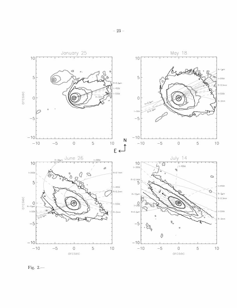
Fig. 2. Contour maps of fragment G (thick grey curves) and the dust model (thick black curves)fitted to the observations. Each successive isophote corresponds to a change in brightness by afactor of 3. The two dimmest observed isophotes are of the image smoothed over a 0.6′′ box. The‘fins’ along the fainter simulated isophotes are an artifact of the model which emits dust havingdiscrete rather than continuous sizes and velocities. The arrow in the July 14 image indicates theprojected direction to Jupiter. Contours for the March fit, which appears similar to the Januaryisophotes, are not displayed. Some isophotes appear incomplete due to rotating the images suchthat north is up. A star trail is responsible for the disagreement in the northwest corner of theJanuary fit. Syndynes (narrow solid curves) are identified by their dust radius R, and synchrones(dashed curves) are shown for dust emitted at times t prior to the observing date. In the January–May images, the smaller, fresh dust inhabit the northern side of the tail, whereas the larger, oldergrains reside on the southern side. In the later observations, the syndynes/synchrones segregatedue to the changing viewing geometry as well as due to proximity to Jupiter.

Fig. 3. Fragment G’s differential dust production rate dN(R) (read with the left axis) and massproduction rate dM(R) (right axis) as a function of grain radius R. Arrows indicate upper limits.The dashed curve has the same logarithmic slope as an R−3.7 Halley–type grain size distribution.These curves assume a dust albedo a = 0.04 and a bulk density of ρd = 1 gm/cm3.

Fig. 4. The dust outflow velocity for fragment G and an R−0.3 curve.

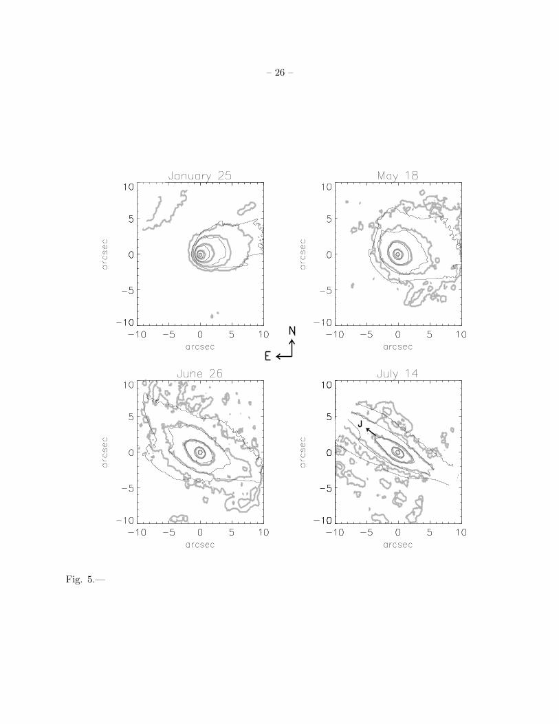
Fig. 5. Contour maps of fragment H (grey curves) and the dust model (black curves) fitted to theobservations. Star trails lie south of the fragment in May, in the southwest corner in June, andnorth of the fragment in July.

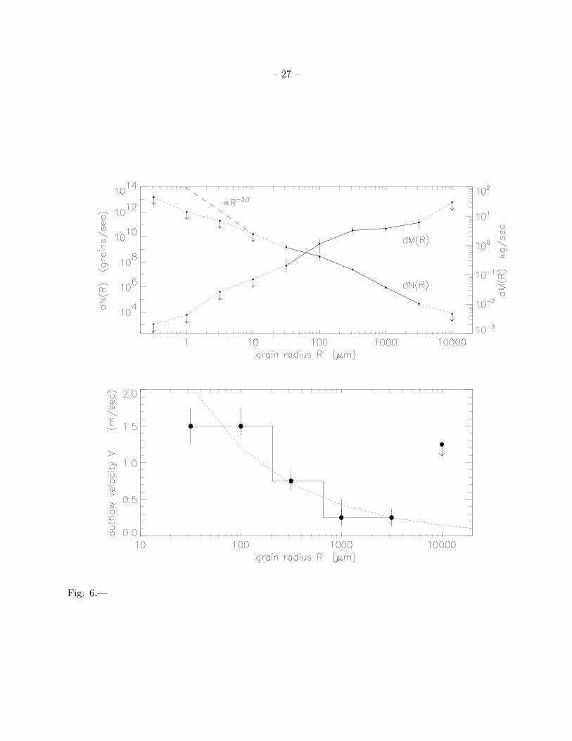
Fig. 6. Fragment H’s differential dust production rate dN(R) and mass production rate dM (R)as a function of grain radius R. Below is the dust outflow velocity distribution V (R) as well as aV (R) ∝ R−b curve with b = 0.5.

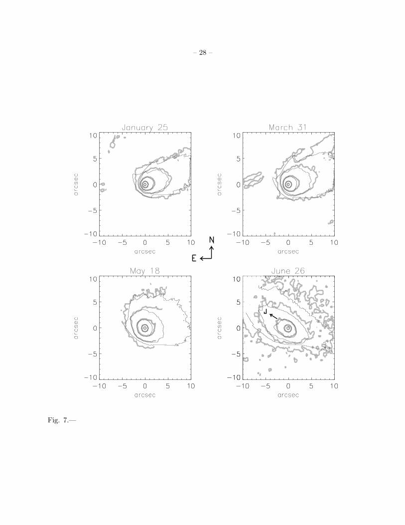
Fig. 7. Contour maps of fragment K (grey curves) and the dust model (black curves) fitted to theobservations. A star trail lies north of the fragment in March, the data were clipped by the detectoredge in May, and this fragment was not observed on July 14.

Fig. 8. Fragment K’s differential dust production rate dN(R) and mass production rate dM (R) asa function of grain radius R, and below a V (R) ∝ R−b curve with b = 0.1 is plotted over the dust

– 19 –

outflow velocity distribution V (R).

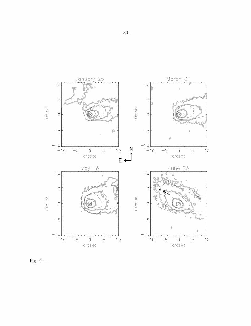
Fig. 9. Contour maps of fragment L (grey curves) and the dust model (black curves) fitted to theobservations. Star trails lie northwest of the fragment in May and west–southwest in June.

Fig. 10. Fragment L’s differential dust production rate dN(R) and mass production rate dM (R)as a function of grain radius R. Below is the dust outflow velocity distribution V (R) as well as aV (R) ∝ R−b curve having b = 0.3.

Fig. 11. Contour maps of fragment S, with fragments T and U indicated in the January image.In the March image a star trail lies at the western edge of the plot, several stars trail through theMay image, and a star trail lies north of the fragment in July.

Fig. 12. The ratio of the surface brightness of fragment S on January 25 to the average of fragmentsG, H, and K, renormalized such that each image has the same integrated brightness as fragment S.Grey areas have a surface brightness ratio of unity, and in the saturated white areas the brightnessof fragment S exceeds the averaged fragments by more than a factor of 1.8. The bullseye indicatesthe coma photocenter, and the white patch to the west is fragment T. The data become spotty asthe signal diminishes with distance down the tail, and the diagram displays only those pixels wherethe flux ratio has a signal/noise> 1.5.

– 20 –

Table I:TABLE I

S–L 9 OBSERVATION PARAMETERSa

Date (1994) IDb rc (AU) ∆d (AU) rJe (106 km) φf (degrees)

January 25 A–W 5.39 5.40 40.0 -10.5March 31 A–W 5.38 4.50 31.2 -5.6May 18 A–W 5.38 4.41 22.8 3.7June 26 H 5.39 4.80 12.1 9.5

S 13.2June 27 K 5.40 4.82 12.2 9.5July 4 Q1 5.40 4.91 10.1 10.0July 12 Q1 5.41 5.03 6.81 10.5July 14 G 5.41 5.07 3.92 10.6

H 4.49S 5.78

July 19 K 5.42 5.14 1.37 10.7July 20 L 5.41 5.16 0.86 10.7

Q1 1.01S 1.90

July 21 S 5.41 5.17 1.49 10.7

aProvided by P.W Chodas (1995, private communication).bFragment ID.

cThe comet’s heliocentric distance.dGeocentric distance.eJovicentric distance.

fSun–comet–Earth phase angle. A minus sign indicates a pre–opposition observation.

– 21 –

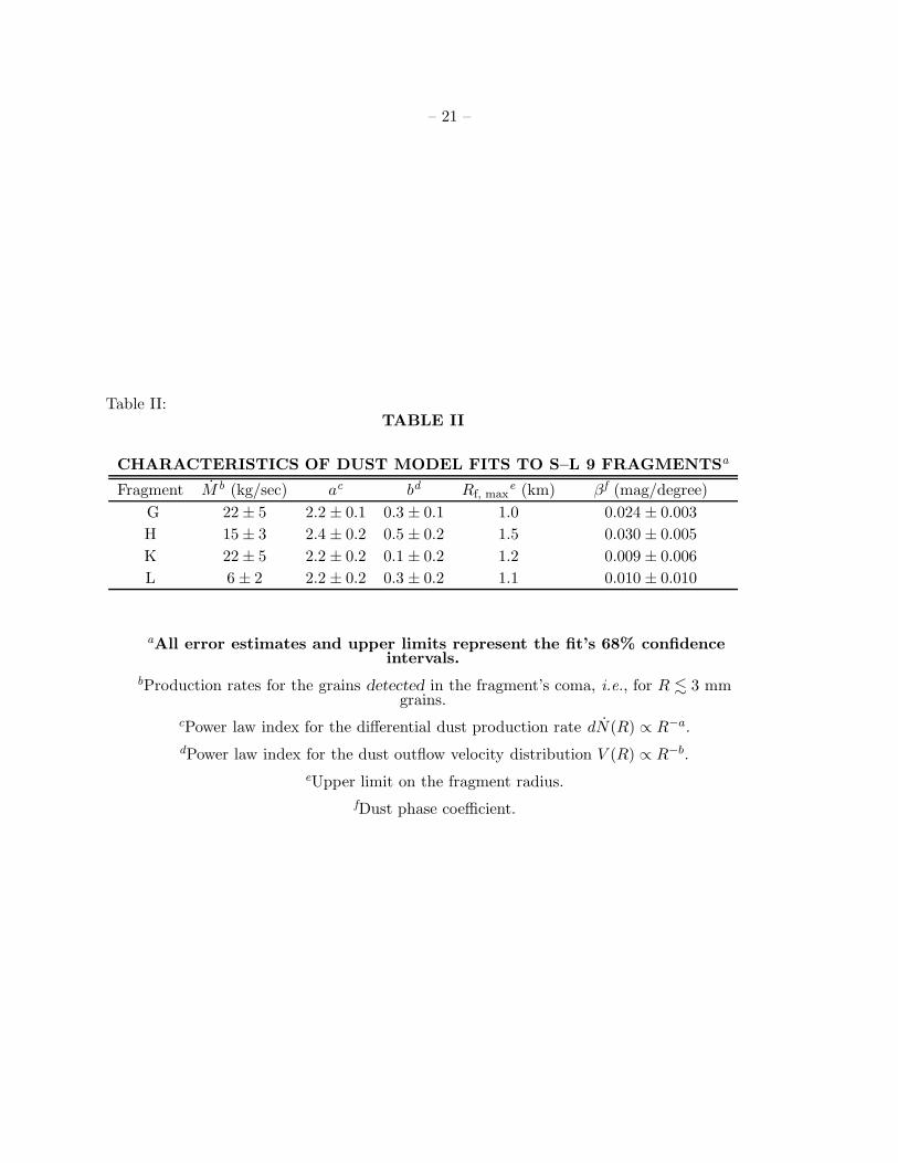
Table II:TABLE II

CHARACTERISTICS OF DUST MODEL FITS TO S–L 9 FRAGMENTSa

Fragment Mb (kg/sec) ac bd Rf, maxe (km) βf (mag/degree)

G 22 ± 5 2.2 ± 0.1 0.3 ± 0.1 1.0 0.024 ± 0.003H 15 ± 3 2.4 ± 0.2 0.5 ± 0.2 1.5 0.030 ± 0.005K 22 ± 5 2.2 ± 0.2 0.1 ± 0.2 1.2 0.009 ± 0.006L 6 ± 2 2.2 ± 0.2 0.3 ± 0.2 1.1 0.010 ± 0.010

aAll error estimates and upper limits represent the fit’s 68% confidenceintervals.

bProduction rates for the grains detected in the fragment’s coma, i.e., for R . 3 mmgrains.

cPower law index for the differential dust production rate dN(R) ∝ R−a.dPower law index for the dust outflow velocity distribution V (R) ∝ R−b.

eUpper limit on the fragment radius.fDust phase coefficient.

– 22 –

Fig. 1.—

– 23 –

Fig. 2.—

– 24 –

Fig. 3.—

– 25 –

Fig. 4.—

– 26 –

Fig. 5.—

– 27 –

Fig. 6.—

– 28 –

Fig. 7.—

– 29 –

Fig. 8.—

– 30 –

Fig. 9.—

– 31 –

Fig. 10.—

– 32 –

Fig. 11.—

– 33 –

Fig. 12.—