COMP9444: Neural Networks Support Vector Machinescs9444/13s2/Notes13/05_SVM.pdf · COMP9444 11s2 Support Vector Machines 8 Geometrical Considerations The support vectors are the ones

COMP9444: Neural Networks

Support Vector Machines

COMP9444 c©Alan Blair, 2011

COMP9444 11s2 Support Vector Machines 1

Optimal Hyperplane

Suppose the training data

(~x1,y1), ...,(~xN ,yN), ~xi ∈ Rm, yi ∈ {−1,+1}

can be separated by a hyperplane

~wT~x+b = 0.

The hyperplane which separates the training data without error and has

maximal distance to the closest training vector is called the Optimal

Hyperplane.



Support Vectors

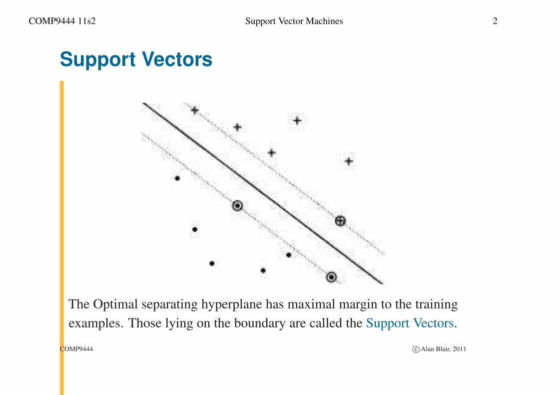
The Optimal separating hyperplane has maximal margin to the training

examples. Those lying on the boundary are called the Support Vectors.



Optimal Hyperplane

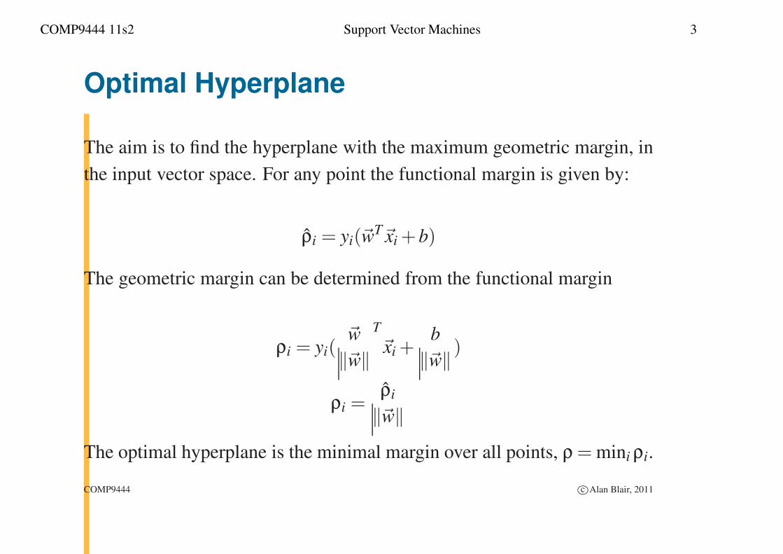
The aim is to find the hyperplane with the maximum geometric margin, in

the input vector space. For any point the functional margin is given by:

ρ̂i = yi(~wT~xi +b)

The geometric margin can be determined from the functional margin

ρi = yi(~w

‖~w‖T

~xi +b

‖~w‖ )

ρi =ρ̂i

‖~w‖The optimal hyperplane is the minimal margin over all points, ρ = mini ρi.



Optimal Hyperplane

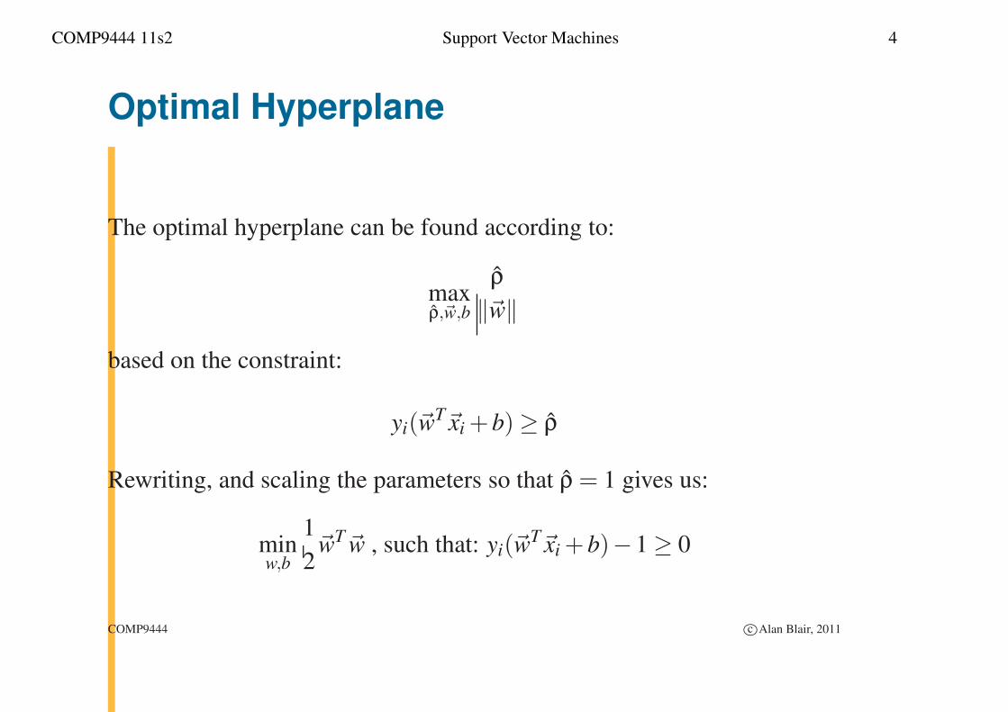
The optimal hyperplane can be found according to:

maxρ̂,~w,b

ρ̂

‖~w‖

based on the constraint:

yi(~wT~xi +b)≥ ρ̂

Rewriting, and scaling the parameters so that ρ̂ = 1 gives us:

minw,b

1

2~wT~w , such that: yi(~w

T~xi +b)−1 ≥ 0



Optimal Hyperplane

The solution can be found using the method of Lagrange multipliers, with

the KKT inequality constraint:

yi(~wT xi +b)−1 ≤ 0

as follows:

L(~w,b,~α) =1

2~wT~w+

N

∑i

αi(yi(~wT xi +b)−1)

The solution for ~w,b is found according to:

max~α,~α≥0

min~w,b

L(~w,b,~α)



Lagrangian Formulation

The parameters αi are known as Lagrange multipliers. The point (~w,b,~α)

is the critical point of the Lagrangian function

L(~w,b,~α) =1

2~wT~w−

N

∑i=1

αi [yi(~wT~xi +b)−1]

=1

2~wT~w−~wT

(

N

∑i=1

αiyi~xi

)

−bN

∑i=1

αiyi +N

∑i=1

αi

L(~α) =N

∑i=1

αi −1

2

N

∑i=1

N

∑j=1

αiα jyiy j~xTi ~x j

There is a duality theorem which allows us to eliminate ~w and b and

compute the α’s directly from the above equation. Notice that the actual

data points~xi appear only in the form of dot products~xTi ~x j.



Primal Problem

The solution can be found according to: max~α L(~α)

subject to the constraints:

N

∑i=1

αiyi = 0, (1)

αi ≥ 0 for i = 1, . . .N (2)

Note: in the more general case where the points are not linearly separable,

but we want to find the best fit we can, condition (2) will be replaced by

0 ≤ αi ≤C,

where C is a regularization parameter which can be determined

experimentally or analytically, using estimate of VC-dim.



Geometrical Considerations

The support vectors are the ones for which the constraint is “tight”, i.e.

yi(~wT~xi +b)−1 = 0

The other data points, i.e. those for which the point (~w,b) does not lie

on the constraint boundary, must have αi = 0. Therefore, the following

product must be zero for all i

αi [yi(~wT~xi +b)−1] = 0

Note also that

~wT~w = ~wT(

N

∑i=1

αiyi~xi

)

=N

∑i=1

N

∑j=1

αiα jyiy j~xTi ~x j



Finding the Optimal Hyperplane

The optimal values for~α can be found by solving the Primal Problem with

quadratic programming techniques.

~w can then be found from

~w =N

∑i=1

αi yi~xi

b can be found from any of the support vectors

(those for which αi 6= 0) by

b = yi −~wT~xi



VC-dim of Optimal Hyperplanes

Consider the following set of training vectors X∗ = {~x1, ..., ~xN}, bounded

by a sphere of radius D, i.e.

|~xi −~a| ≤ D, xi ∈ X∗,

where ~a is the centre of the sphere.

Theorem (Vapnik, 1995) A subset of canonical hyperplanes

f (~x,~w,b) = sign((~wT~x)+b),

defined on X∗ and satisfying the constraint ||~w|| ≤ A has VC-dimension h

bounded by the inequality

h ≤ min([D2A2],m)+1,

m being the number of dimensions.



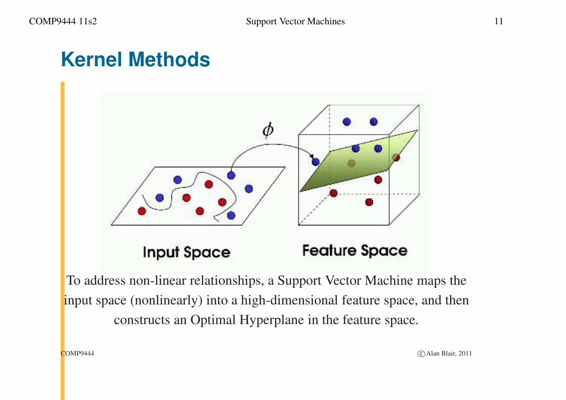
Kernel Methods

To address non-linear relationships, a Support Vector Machine maps the

input space (nonlinearly) into a high-dimensional feature space, and then

constructs an Optimal Hyperplane in the feature space.




Two problems:

• How to find a separating hyperplane that will generalise well?

The dimensionality of the feature space will be very large. As

a consequence, not all separating hyperplanes will generalise

well.

• How to treat computationally such high-dimensional spaces?

A very high-dimensional feature space cannot be explicitly

computed. e.g. considering polynomials of degree 4 or 5 in a

200 dimensional input space results in a billion dimensional

feature space. Obviously, “special” treatment of such spaces is

required.



The Kernel Trick

The features (φ1(~x), . . . ,φm(~x)) will play the same role that was previously

played by the co-ordinates of ~x. By convention, we add an additional

“bias” feature φ0() with φ0(~x) = 1 for all~x. Recall that we only need to be

able to compute the dot products

K(~xi,~x j) =~φ T(~xi)~φ(~x j) =m

∑k=0

φk(~xi)φk(~x j).

Fortunately K(~xi,~x j), which is known as a Kernel function, can often be

computed directly without having to compute the individual φk’s. This is

the key idea which makes Support Vector Machines computable.



Polynomial Features

For example, if~φ() is the set of polynomials in x1, . . . ,xl

of degree up to p, then

K(~x,~y) = (1+~xT~y) p

e.g. if l = 2 and p = 2,

K(~x,~y) = (1+ x1y1 + x2y2)2

= 1+2x1y1 +2x2y2 + x21y2

1 +2x1x2y1y2 + x22y2

2

=m

∑k=0

φk(~x)φk(~y) =~φ T(~x)~φ(~y)

where

~φ(~x) = (1,√

2x1,√

2x2, x21,√

2x1x2, x22 )



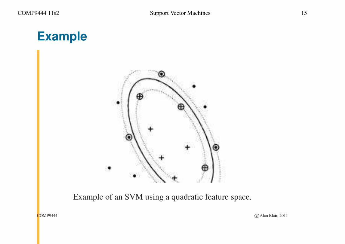
Example

Example of an SVM using a quadratic feature space.



Other Popular Kernel Functions

Radial Basis Function machine:

K(~x,~y) = exp(−||~x−~y||22σ2

)

Two-layer perceptron machine:

K(~x,~y) = tanh(c(~xT~y)−b)

These kernels are not quite well behaved from the point-of-view of

theoretical mathematics (in fact, the RBF kernel corresponds to an

infinite-dimensional feature space). Despite this, they tend to give good

performance in practice.

The tanh kernel can be seen as an alternative to the backpropagation

algorithm, which additionally tells you the number of hidden nodes (equal

to the number of support vectors).




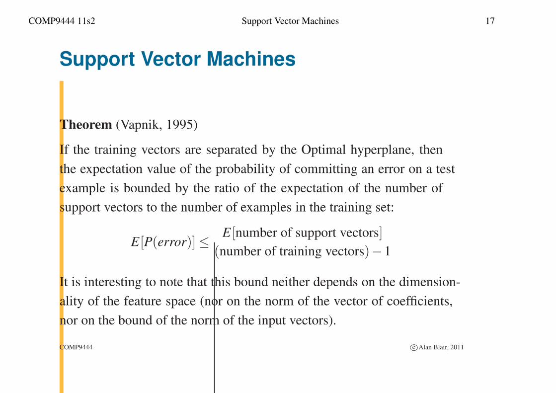
Theorem (Vapnik, 1995)

If the training vectors are separated by the Optimal hyperplane, then

the expectation value of the probability of committing an error on a test

example is bounded by the ratio of the expectation of the number of

support vectors to the number of examples in the training set:

E[P(error)]≤ E[number of support vectors]

(number of training vectors)−1

It is interesting to note that this bound neither depends on the dimension-

ality of the feature space (nor on the norm of the vector of coefficients,

nor on the bound of the norm of the input vectors).




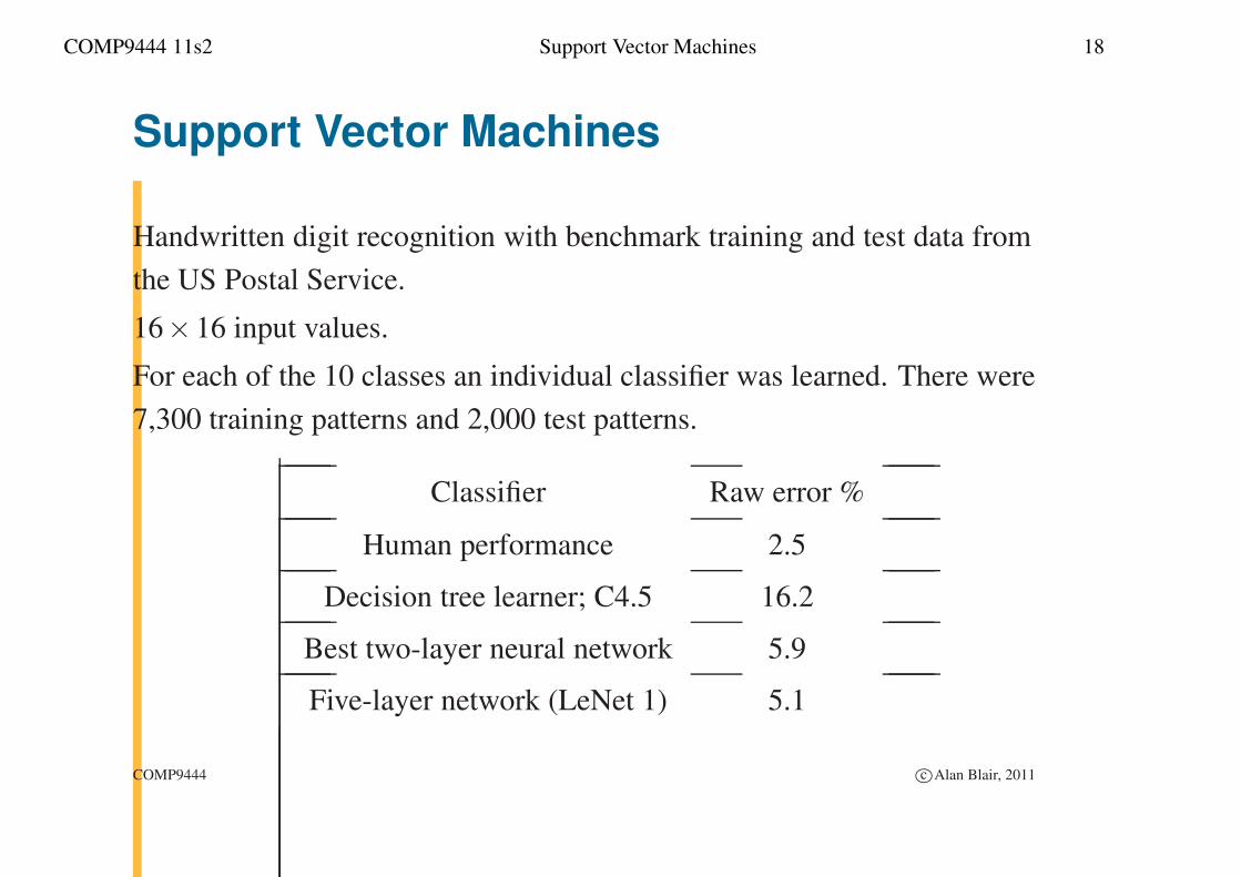
Handwritten digit recognition with benchmark training and test data from

the US Postal Service.

16×16 input values.

For each of the 10 classes an individual classifier was learned. There were

7,300 training patterns and 2,000 test patterns.

Classifier Raw error %

Human performance 2.5

Decision tree learner; C4.5 16.2

Best two-layer neural network 5.9

Five-layer network (LeNet 1) 5.1




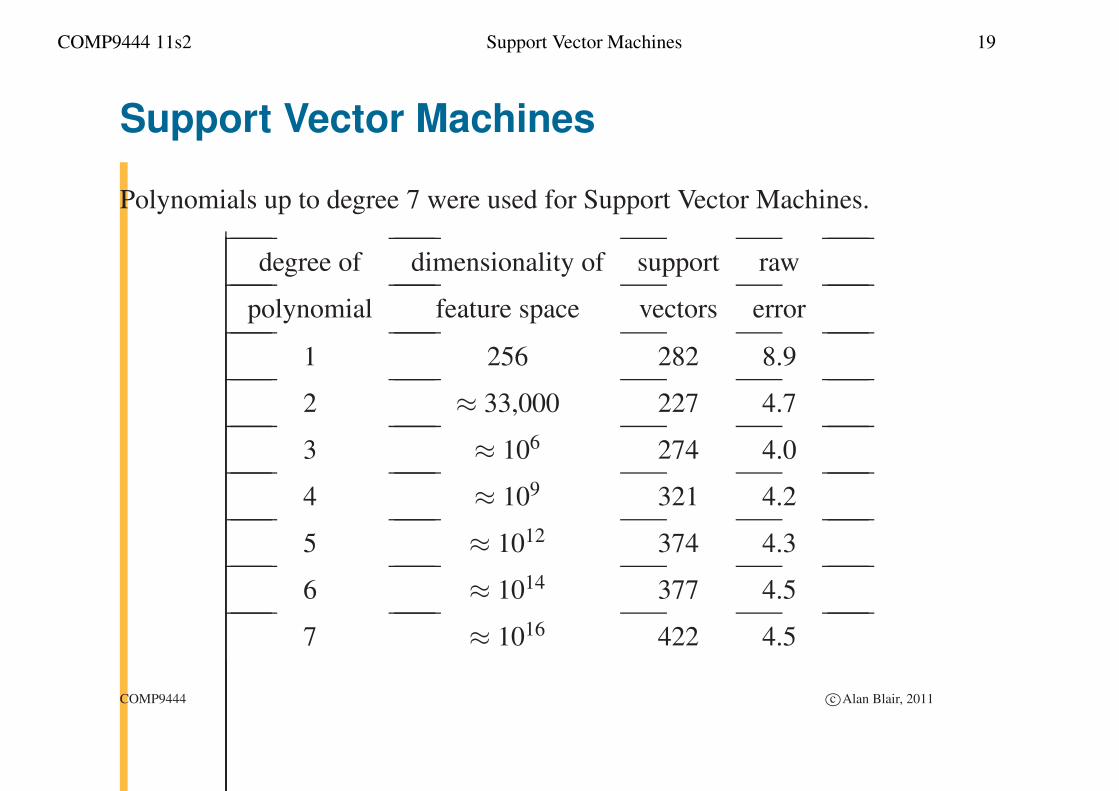
Polynomials up to degree 7 were used for Support Vector Machines.

degree of dimensionality of support raw

polynomial feature space vectors error

1 256 282 8.9

2 ≈ 33,000 227 4.7

3 ≈ 106 274 4.0

4 ≈ 109 321 4.2

5 ≈ 1012 374 4.3

6 ≈ 1014 377 4.5

7 ≈ 1016 422 4.5




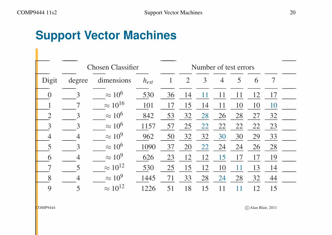
Chosen Classifier Number of test errors

Digit degree dimensions hest 1 2 3 4 5 6 7

0 3 ≈ 106 530 36 14 11 11 11 12 17

1 7 ≈ 1016 101 17 15 14 11 10 10 10

2 3 ≈ 106 842 53 32 28 26 28 27 32

3 3 ≈ 106 1157 57 25 22 22 22 22 23

4 4 ≈ 109 962 50 32 32 30 30 29 33

5 3 ≈ 106 1090 37 20 22 24 24 26 28

6 4 ≈ 109 626 23 12 12 15 17 17 19

7 5 ≈ 1012 530 25 15 12 10 11 13 14

8 4 ≈ 109 1445 71 33 28 24 28 32 44

9 5 ≈ 1012 1226 51 18 15 11 11 12 15



Summary

� The Support Vector Machine (SVM) is an elegant and highly

principled learning method which selects relevant features from a

very high dimensional feature space.

� SVM’s use quadratic programming techniques to solve a constrained

optimization problem, thus avoiding the need to deal directly with the

high dimensional feature space.

� SVM’s run only in batch mode, can’t be trained incrementally.

� Training times for SVM’s are slower than backpropagation, because

there is no control over the number of potential support vectors, and

there is no natural way to incorporate prior knowledge about the task.


Documents

COMP9444: Neural Networks Support Vector Machinescs9444/13s2/Notes13/05_SVM.pdf · COMP9444 11s2 Support Vector Machines 8 Geometrical Considerations The support vectors are the ones