Jan 23 2001:

Comparative advantage and economic geography:estimating the determinants of industrial location in the EU. *

Karen Helene Midelfart-KnarvikNHH, Bergen and CEPR

Henry G. OvermanLSE and CEPR

Anthony J. VenablesLSE and CEPR

Abstract:Wedevelopandeconometricallyestimateamodelofthelocationofindustriesacrosscountries. Themodelcombinesfactorendowmentsandgeographicalconsiderations,andshowshowindustryandcountrycharacteristicsinteracttodeterminethelocationofproduction. WeestimatethemodelonsectoraldataforEUcountriesovertheperiod1980-97,andfindthatendowmentsofskilledandscientificlabourareimportantdeterminantsofindustrialstructure,asalsoareforwardandbackwardlinkages to industry.

JEL number: F10Keywords: specialization, comparative advantage, economic geography.

* ThispaperisproducedaspartoftheGlobalizationprogrammeoftheESRCfundedCentreforEconomicPerformanceattheLSE. ThankstoG.Ottaviano,D.Puga,S.Redding,P.Seabright,D.TreflerandseminarparticipantsatLSE,Toronto,NHH(Bergen),IUI(Stockholm),theEuropeanResearchWorkshoponInternationalTrade(Copenhagen),and the Empirical Investigations in International Trade Conference (Boulder).

Authors’ addresses:K.H. Midelfart-KnarvikDept of EconomicsNorwegianSchoolofEconomicsandBusiness AdministrationHelleveien 305045 Bergen, NorwayKarenHelene.Knarvik@snf.no

H.G. OvermanDept of GeographyLSEHoughton StreetLondon WC2A 2AE

h.g.overman@lse.ac.uk

A.J. VenablesDept of EconomicsLSEHoughton StreetLondon WC2A 2AE

a.j.venables@lse.ac.uk

1

1. Introduction

Thispaperaddressesthequestion:whatdeterminesthelocationofdifferentindustriesacrosscountries? Theorytellsus

thatitdependsonsupplyconsiderations,onthecross-countrydistributionofdemandforeachsector’soutput,andon

theeaseoftrade. Inthecaseinwhichtradeisperfectlyfree,thenthedistributionofdemandbecomesunimportantand

supplyalonedeterminesthelocationofproduction. Thisisthebasisofthetextbookmodelsinwhichcomparative

advantage(asdrivenbytechnologyorendowmentdifferences)determinesthestructureofproductionineachcountry.

Moregenerally,thepresenceoftransportcostsorothertradefrictionsmeanthatbothsupplyanddemandmatter. If

transportcostsvarysystematicallywithdistancethengeographicalfactorscomeintoplay,combiningwithcomparative

advantage to determine industrial location.

Theobjectiveofthispaperistodevelopandeconometricallyestimateamodelcombiningcomparative

advantageandgeographicalforces.1 Ourmodelcontainscountriesthathavedifferingfactorendowmentsandface

transportcostsontheirtrade. Industrialsectorsuseprimaryfactorsandintermediategoodstoproducedifferentiated

goods,differentiationensuringthattherearepositivetradeflows,despitetransportcosts. Theequilibriumpatternof

industriallocationisdeterminedbothbyfactorendowmentsandgeography. Factorendowmentsmatterfortheusual

reasons,althoughfactorpricesarenotgenerallyequalizedbytrade. Transportcostsmeanthatthelocationofdemand

matters;countriesatdifferentlocationshavedifferentmarketpotential,andthisshapestheirindustrial structures.

Intermediategoodspricesanddemandvaryacrosslocations,meaningthatforwardandbackwardlinkageeffectsare

present and that industries will tend to locate close to supplier and customer industries.

Ourtaskistocombinetheseeffectsandshowhowtheyimpactdifferentlyondifferentsectors. Allindustries

would,otherthingsbeingequal,tendtolocateincountrieswithabundantfactorsupplies,goodmarketaccess,and

proximitytosuppliers. Ingeneralequilibrium,whatarethecharacteristicsof industriesthatleadthemtolocatein

countriesofdifferenttypes? Weillustratetheanswertothis,showinghowitispossibletogeneralisetheRybczynskiand

Heckscher-Ohlineffectsofstandardmodels. Wethenlinearisethemodel,andshowhowcharacteristicsofcountries

(suchastheirendowmentsorlocation)interactwithcharacteristicsof industries(suchastheir factorintensityor

transport costs) to determine production structure. This linearisation provides the equation that we estim

Estimationisundertakenusingdatafor33industriesand14EuropeanUnioncountries,fortheperiod1980-97.

Thisdatasethastheadvantagesofhavingarelativelystraightforwardgeography–withaclearsetofcentraland

peripheralcountries–andofcoveringaperiodofincreasingeconomicintegration. Studiesofproductionfindevidence

thatthespecializationofEuropeancountrieshasincreasedthroughthisperiod.2 Weareabletoprovidesomeinsight

into the roles of comparative advantage and geography in driving these changes.

Ourapproachcanbeviewedasbothasynthesisandageneralization(insomedirections)oftwoapproachesin

2

theexistingempiricalliterature. Thereisasizeableliterature(datingfromBaldwin1971)thatestimatestheeffectof

industrycharacteristicsontrade,runningcross-industryregressionsforasinglecountry.3 Amorerecentliterature(for

exampleLeamer1984,Harrigan1995,1997)estimatestheeffectofcountrycharacteristics(endowmentsandpossibly

alsotechnology)ontradeandproduction,runningcross-countryregressionsandestimatingindustrybyindustry. Our

approachtakesthepanelofindustriesandcountries,andestimatesthewayinwhichproductiondependsonboth

industrycharacteristicsandcountrycharacteristics,withtheformoftheinteractionbetweentheseeffectsdictatedby

theory. ThisapproachisperhapsclosesttoEllisonandGlaeser(1999)whoanalysehowindustriallocationinUSstates

isaffectedbyarangeof ‘naturaladvantages’. OurpaperdiffersfromEllisonandGlaeserinderivingthetheoretical

specificationfromtrade,ratherthanlocation,theory. Asaresult,ourinteractionsmoreclearlyrelatebothtocountries’

factor endowments and to their relative locations.

RecentworkbyDavisandWeinstein(1998,1999)combinescomparativeadvantageandgeographybyassuming

thatthebroadsectoralpatternofspecialization(3digit)isdeterminedbyendowments,andthefinerdetailof4digit

productiondeterminedbyeithergeographyorendowments. Theyinvestigatetheeffectofdemandshocksonproduction,

inordertotestforhomemarketeffects. Ourmodeldoesnotmakethistwolevelseparation,andthequestionweaddress

isbroader,insofaraswearelookingathowavarietyofdifferentforcesinteracttodeterminelocation. However,our

modelisnarrowerthanDavisandWeinstein’sinsofarasweassumethroughoutthatallsectorsareperfectlycompetitive.

Whilegeographycan,ofcourse,haveabearingonindustrial locationinacompetitiveenvironment,thisrestriction

meansthatsomeoftheforcesofneweconomicgeographyareabsentfromourapproach. Wemakethisassumptionin

ordertohaveapreciseandtractable linkbetweenthetheoryandtheeconometrics,whereasaddingimperfect

competitionwouldraiseanumberof issueswhichgobeyondthescopeof thispaper. Forexample, insuchan

environmenttheremaybeamultiplicityofequilibria,andhencenouniquemappingfromunderlyingcharacteristicsof

countries and industries to industrial location4. Addressing these issues will be the subject of future researc

Thepaperproceedsasfollows. Section2outlinestheanalyticalframework,andsection3derivesourestimating

equation. Section4discussestheinteractionsinthisequation,andsection5presentseconometricresults. Section6

concludes.

2. The model

ThemodelcontainsIcountries,KindustrialsectorsandMprimaryfactors. Allindustriesareperfectlycompetitiveand

haveconstantreturnstoscale,usingprimaryfactorsandintermediategoodsasinputs. Eachindustryproducesanumber

ofvarietiesofdifferentiatedproducts;wedenotethenumberofvarietiesproducedincountry ibyindustrykbynik,and

assumethatthisisdeterminedexogenously. Goodsaretradeablebutincurtransportcosts,thelevelofwhichisindustry

3

(1)

(2)

(3)

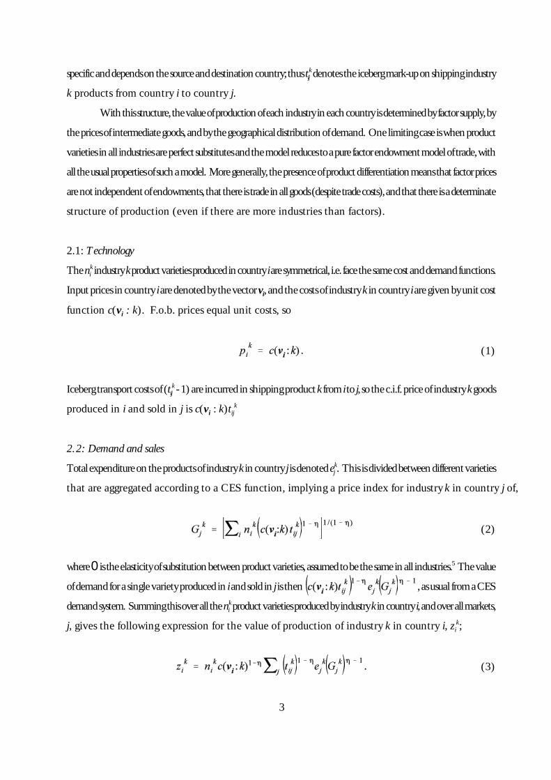
specificanddependsonthesourceanddestinationcountry;thustijkdenotestheicebergmark-uponshippingindustry

k products from country i to country j.

Withthisstructure,thevalueofproductionofeachindustryineachcountryisdeterminedbyfactorsupply,by

thepricesofintermediategoods,andbythegeographicaldistributionofdemand. Onelimitingcaseiswhenproduct

varietiesinallindustriesareperfectsubstitutesandthemodelreducestoapurefactorendowmentmodeloftrade,with

alltheusualpropertiesofsuchamodel. Moregenerally,thepresenceofproductdifferentiationmeansthatfactorprices

arenotindependentofendowments,thatthereistradeinallgoods(despitetradecosts),andthatthereisadeterminate

structure of production (even if there are more industries than factors).

2.1: Technology

Thenik industrykproductvarietiesproducedincountry iaresymmetrical,i.e.facethesamecostanddemandfunctions.

Inputpricesincountry iaredenotedbythevectorvi,andthecostsof industryk incountry iaregivenbyunitcost

function c(vi : k). F.o.b. prices equal unit costs, so

Icebergtransportcostsof(tijk -1)areincurredinshippingproductk from ito j, sothec.i.f.priceof industrykgoods

produced in i and sold in j is c(vi : k)tijk

2.2: Demand and sales

Totalexpenditureontheproductsofindustryk incountry j isdenotedejk. Thisisdividedbetweendifferentvarieties

that are aggregated according to a CES function, implying a price index for industry k in country j of,

where0istheelasticityofsubstitutionbetweenproductvarieties,assumedtobethesameinallindustries.5 Thevalue

ofdemandforasinglevarietyproducedin iandsoldin j isthen ,asusualfromaCES

demandsystem. Summingthisoverallthenikproductvarietiesproducedbyindustrykincountryi,andoverallmarkets,

j, gives the following expression for the value of production of industry k in country i, zik;

4

(4)

(5)

(6)

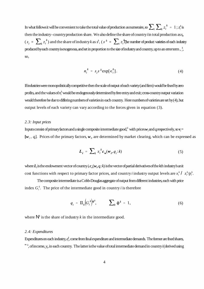
Inwhatfollowsitwillbeconvenienttotakethetotalvalueofproductionasnumeraire,so ; zik is

thenthe industry -countryproduction share. Wealsodefinetheshareof country i in totalproductionas si,

( ) and the share of industry k as sk, ( ).The number of product varieties of each industry

producedbyeachcountryisexogenous,andsetinproportiontothesizeofindustryandcountry,uptoanerrorterm,ik,

so,

Ifindustriesweremonopolisticallycompetitivethenthescaleofoutputofeachvariety(andfirm)wouldbefixedbyzero

profits,andthevaluesofnikwouldbeendogenouslydeterminedbyfreeentryandexit;cross-countryoutputvariation

wouldthereforebeduetodifferingnumbersofvarietiesineachcountry. Herenumbersofvarietiesaresetby(4),but

output levels of each variety can vary according to the forces given in equation (3).

2.3: Input prices

Inputsconsistofprimaryfactorsandasinglecompositeintermediategood,6 withpriceswiandqirespectively,sovi=

[wi , qi]. Prices of the primary factors, wi, are determined by market clearing, which can be expressed as

whereLi istheendowmentvectorofcountry i,cw(wi,qi :k)isthevectorofpartialderivativesofthekthindustry’sunit

cost functions with respect to primary factor prices, and country i industry output levels are xik / zi

k/pik.

ThecompositeintermediateisaCobb-Douglasaggregateofoutputfromdifferentindustries,eachwithprice

index Gik. The price of the intermediate good in country i is therefore

where Nk is the share of industry k in the intermediate good.

2.4: Expenditures

Expendituresoneachindustry,eik,comefromfinalexpenditureandintermediatedemands. Theformerarefixedshares,

"k,of income,yi, ineachcountry. Thelatter isthevalueoftotalintermediatedemandincountry i(derivedusing

5

(7)

(8)

(9)

(10)

Shephard’s lemma on industry cost functions) times the share attributable to sector k, Nk,

Income, yi, is derived from primary factors in the usual way.

3. Estimating equation

Ourestimatingequationisbasedontheoutputofeachindustryineachcountry,expressedrelativetothesizeofthe

industry and the country. We denote this double relative measure rik, and using (3) and (4) it takes the fo

Theterminthesummationsigncapturesdemandeffects,andwerefertotheseasthemarketpotentialofindustrykin

country i. We shall denote this m(uk : i),

Themarketpotentialfunction,m(uk : i),isindexedacrosscountries,i,andthevectorukreferstoindustrycharacteristics

thatinteractwiththespatialdistributionofdemand(suchastransportcosts;wediscusstheseinthenextsection).

Equation (8), for the output of each industry in each country, now becomes

Thissaysthatsystematiccross-countryvariationinsectors’outputisdeterminedbytwosortsofconsiderations. Oneis

inputpricevariation,capturedintheunitcostfunction. Theotherisdemandvariation,capturedbythemarketpotential

of industry k in country i.7

Toestimatethemodelwelog-lineariseequation(10)aroundareferencepoint. Thisissimplifiedbynotingthat

thefunctionsc(vi :k)andm(uk : i)canbeconstructedsuchthat:(i)thereexistsaninputpricevector, ,atwhich

forallindustriesk,and:(ii)thereexistsavectorofindustrycharacteristics, ,suchthat

forallcountries i8.Thesedefineourreferencecountryandindustry. Linearising(7)aroundthereferencepointgives

6

(11)

(12)

(13)

(14)

where)denotesaproportionatechange,e.g. ;

isthe(row)vectorofelasticitiesofindustrykcostswithrespecttoinputprices,vi,(theseelasticitiesalsobeingtheshare

ofeachinputincosts);and isthevectorofelasticitiesofcountry imarketpotentialwith

respect to industry characteristics, uk.9

Sincetherikareshares,deviationsmustsatisfyanaddingupcondition, . Usingthis

with equation (11) gives

The double summation terms in (12) do not vary over either industries or countries, so we write

Termsontherighthandsideof(13)aretheproductofcountryandindustrycharacteristics,bothexpressedindeviation

form. Thefirstinnerproductgivescountries’inputpricestimesindustries’inputshares(elasticitiesofcostswithrespect

toinputprices). Thesecondgivesindustries’characteristicstimeselasticitiesofcountries’marketpotentialswithrespect

tothesecharacteristics. Intheeconometricimplementationofthemodelweusesixinteractions,andwenowexplore

each of these in turn.

4. Interactions

4.1: Primary factors;

Onthecost side, inputpricesincludebothprimaryfactorpricesandintermediatesgoodprices,partitionedinto

. The corresponding vector of input shares is .

Forprimaryfactorswegobackto factorendowmentsratherthanusefactorprices, sincethelatterare

endogenous. The vector of factor price variations, ))))wi, depends on endowments according to

7

(15)

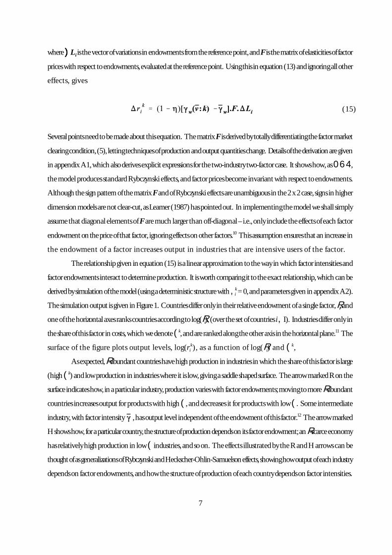
where))))Liisthevectorofvariationsinendowmentsfromthereferencepoint,andFisthematrixofelasticitiesoffactor

priceswithrespecttoendowments,evaluatedatthereferencepoint. Usingthisinequation(13)andignoringallother

effects, gives

Severalpointsneedtobemadeaboutthisequation. ThematrixFisderivedbytotallydifferentiatingthefactormarket

clearingcondition,(5),lettingtechniquesofproductionandoutputquantitieschange. Detailsofthederivationaregiven

inappendixA1,whichalsoderivesexplicitexpressionsforthetwo-industrytwo-factorcase. Itshowshow,as064,

themodelproducesstandardRybczynskieffects,andfactorpricesbecomeinvariantwithrespecttoendowments.

AlthoughthesignpatternofthematrixFandofRybczynskieffectsareunambiguousinthe2x2case,signsinhigher

dimensionmodelsarenotclear-cut,asLeamer(1987)haspointedout. Inimplementingthemodelweshallsimply

assumethatdiagonalelementsofFaremuchlargerthanoff-diagonal–i.e.,onlyincludetheeffectsofeachfactor

endowmentonthepriceofthatfactor,ignoringeffectsonotherfactors.10 Thisassumptionensuresthatanincreasein

the endowment of a factor increases output in industries that are intensive users of the factor.

Therelationshipgiveninequation(15)isalinearapproximationtothewayinwhichfactorintensitiesand

factorendowmentsinteracttodetermineproduction. Itisworthcomparingittotheexactrelationship,whichcanbe

derivedbysimulationofthemodel(usingadeterministicstructurewith,ik=0,andparametersgiveninappendixA2).

ThesimulationoutputisgiveninFigure1. Countriesdifferonlyintheirrelativeendowmentofasinglefactor,Ri,and

oneofthehorizontalaxesrankscountriesaccordingtolog(Ri),(overthesetofcountries i,I). Industriesdifferonlyin

theshareofthisfactorincosts,whichwedenote(k,andarerankedalongtheotheraxisinthehorizontalplane.11 The

surface of the figure plots output levels, log(rik), as a function of log(Ri) and (k,

Asexpected,R-abundantcountrieshavehighproductioninindustriesinwhichtheshareofthisfactorislarge

(high(k)andlowproductioninindustrieswhereitislow,givingasaddleshapedsurface. ThearrowmarkedRonthe

surfaceindicateshow,inaparticularindustry,productionvarieswithfactorendowments;movingtomoreR-abundant

countriesincreasesoutputforproductswithhigh(,anddecreasesit forproductswithlow(. Someintermediate

industry,withfactorintensity ,hasoutputlevelindependentoftheendowmentofthisfactor.12 Thearrowmarked

Hshowshow,foraparticularcountry,thestructureofproductiondependsonitsfactorendowment;anR-scarceeconomy

hasrelativelyhighproductioninlow( industries,andsoon. TheeffectsillustratedbytheRandHarrowscanbe

thoughtofasgeneralizationsofRybczynskiandHeckscher-Ohlin-Samuelsoneffects,showinghowoutputofeachindustry

dependsonfactorendowments,andhowthestructureofproductionofeachcountrydependsonfactorintensities.

8

(16)

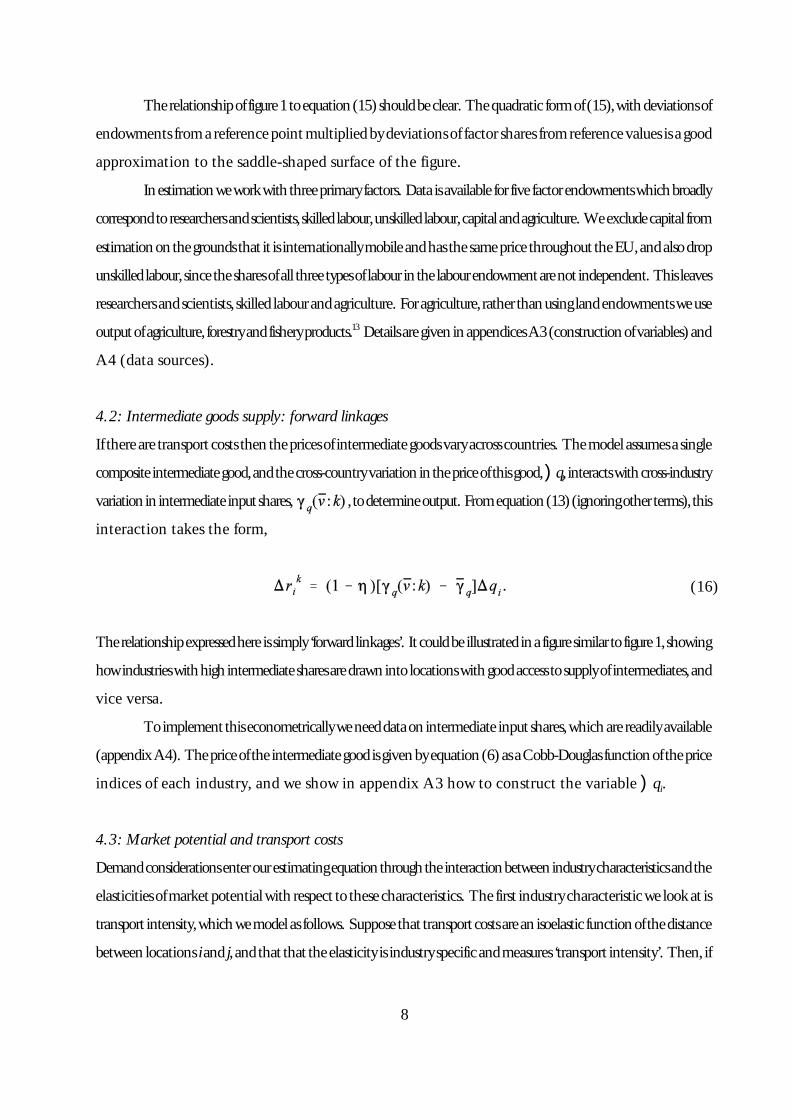
Therelationshipoffigure1toequation(15)shouldbeclear. Thequadraticformof(15),withdeviationsof

endowments fromareferencepointmultipliedbydeviationsof factor shares fromreferencevalues isagood

approximation to the saddle-shaped surface of the figure.

Inestimationweworkwiththreeprimaryfactors. Dataisavailableforfivefactorendowmentswhichbroadly

correspondtoresearchersandscientists,skilledlabour,unskilledlabour,capitalandagriculture. Weexcludecapitalfrom

estimationonthegroundsthatitisinternationallymobileandhasthesamepricethroughouttheEU,andalsodrop

unskilledlabour,sincethesharesofallthreetypesoflabourinthelabourendowmentarenotindependent. Thisleaves

researchersandscientists,skilledlabourandagriculture. Foragriculture,ratherthanusinglandendowmentsweuse

outputofagriculture,forestryandfisheryproducts.13 DetailsaregiveninappendicesA3(constructionofvariables)and

A4 (data sources).

4.2: Intermediate goods supply: forward linkages

If therearetransportcoststhenthepricesofintermediategoodsvaryacrosscountries. Themodelassumesasingle

compositeintermediategood,andthecross-countryvariationinthepriceofthisgood,)qi,interactswithcross-industry

variationinintermediateinputshares, ,todetermineoutput. Fromequation(13)(ignoringotherterms),this

interaction takes the form,

Therelationshipexpressedhereissimply‘forwardlinkages’. Itcouldbeillustratedinafiguresimilartofigure1,showing

howindustrieswithhighintermediatesharesaredrawnintolocationswithgoodaccesstosupplyofintermediates,and

vice versa.

Toimplementthiseconometricallyweneeddataonintermediateinputshares,whicharereadilyavailable

(appendixA4). Thepriceoftheintermediategoodisgivenbyequation(6)asaCobb-Douglasfunctionoftheprice

indices of each industry, and we show in appendix A3 how to construct the variable )qi.

4.3: Market potential and transport costs

Demandconsiderationsenterourestimatingequationthroughtheinteractionbetweenindustrycharacteristicsandthe

elasticitiesofmarketpotentialwithrespecttothesecharacteristics. Thefirst industrycharacteristicwelookatis

transportintensity,whichwemodelasfollows. Supposethattransportcostsareanisoelasticfunctionofthedistance

betweenlocations iand j,andthatthattheelasticityisindustryspecificandmeasures‘transportintensity’. Then,if

9

(17)

(18)

distance is denoted dij, and the transport intensity of industry k, 2k, we have

EstimatesoftransportintensityareobtainedfromtheGTAPmodellingproject(seeappendixA3). Usingthisexpression,

the market potential of industry k in country i (equation (9)), becomes

Linearizationrequiresthatwefindtheelasticityofthiswithrespecttotransportintensity,evaluatedforsomereference

industry. Details of the procedure for doing this are given in appendix A3.

Figure2showshowtransportintensityinteractswithmarketpotentialtodetermineindustriallocation. The

figureiscomputedforanexampleinwhichtheonlydifferencebetweenindustriesisintransportintensity,andtheonly

differencebetweencountriesisthatsomeareclosertoothermarketssohavehighermarketpotential. Thefigureplots

outthesurfaceoflog(rik)againstindustries’transportintensitiesandcountries’computedmarketpotentials. Forthe

rangeoftransportintensitiesshownthesurfaceissaddle-shapedand,asexpected,productioninhightransportintensity

industriestendstoconcentrateincountrieswithhighmarketpotential. However,weshouldnotethatthissaddleshape

isnotaglobalpropertyofthesurface–anon-tradableindustrywouldevidentlyhaveproductiondeterminedsolelyby

local demand, not by countries’ reference market potential.14

4.4: Intermediate goods demand; Backward linkages

Transportintensityisnottheonlyindustrycharacteristicthatinteractswithcountries’location. Afurtherinteraction

arisesfromthefactthatthespatialpatternofdemand,eik,maydifferacrossindustries. Thiscouldinprinciplebedue

tofinalexpendituredifferences,althoughtheidenticalhomotheticstructureofpreferencesembodiedinequation(7)

rulesthisout. Alternatively,itmaybeduetothespatialdistributionofderiveddemandvaryingacross industries--

backwards linkages. We expect upstream industries to locate in countries in which derived demand is hig

Asusual,equation(13)saysthatthisshouldbemodelledasaninteractionbetweenanindustrycharacteristic

andacountrycharacteristic. Theindustrycharacteristicistheshareofeachindustry’soutputthatgoesforintermediate

usage. Thecountrycharacteristicistheelasticityofmarketpotentialwithrespecttothisshare,whichturnsoutto

dependonthedifferencebetweenamarketpotentialbasedonfinalexpenditureandamarketpotentialbasedon

intermediateexpenditures(derivedinappendixA3). Interactingthesegivesrisetotheusualsaddleshapedrelationship,

10

(19)

(20)

withupstreamindustrieswantingtolocateincountriesinwhichthemarketpotentialfromintermediatesalesishigh

relative to the market potential from final sales.

5. Estimation

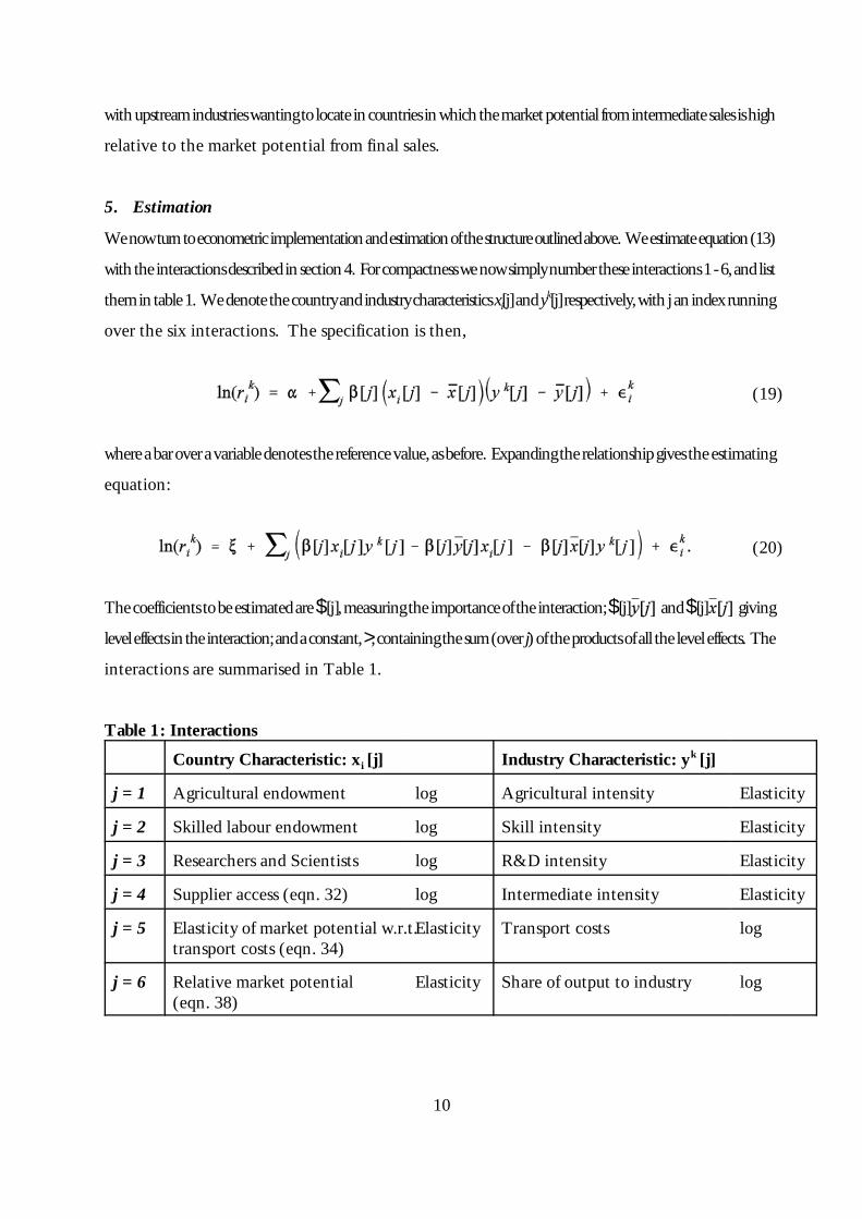
Wenowturntoeconometricimplementationandestimationofthestructureoutlinedabove. Weestimateequation(13)

withtheinteractionsdescribedinsection4. Forcompactnesswenowsimplynumbertheseinteractions1-6,andlist

themintable1. Wedenotethecountryandindustrycharacteristicsxi[j]andyk[j]respectively,withjanindexrunning

over the six interactions. The specification is then,

whereabaroveravariabledenotesthereferencevalue,asbefore. Expandingtherelationshipgivestheestimating

equation:

Thecoefficientstobeestimatedare$[j],measuringtheimportanceoftheinteraction;$[j] and$[j] giving

leveleffectsintheinteraction;andaconstant,>,containingthesum(over j)oftheproductsofalltheleveleffects. The

interactions are summarised in Table 1.

Table 1: Interactions

Country Characteristic: xi [j] Industry Characteristic: yk [j]

j = 1 Agricultural endowment log Agricultural intensity Elasticity

j = 2 Skilled labour endowment log Skill intensity Elasticity

j = 3 Researchers and Scientists log R&D intensity Elasticity

j = 4 Supplier access (eqn. 32) log Intermediate intensity Elasticity

j = 5 Elasticity of market potential w.r.t.transport costs (eqn. 34)

Elasticity Transport costs log

j = 6 Relative market potential(eqn. 38)

Elasticity Share of output to industry log

11

5.1 Data and estimation:

Ourdataisfor14EUcountriesand36manufacturingindustries,althoughweomitthreesectors–petroleumrefineries,

petroleumandcoalproducts(whoselocationispredominantlynaturalresourcedriven)andmanufacturingnotelsewhere

classified-essentiallyaresidualcomponent. Wehavedataonoutputfrom1980-1997,butbecausewecannotgetfull

timeseriesforalltheindependentvariables,wepickfourtimeperiods.15 Withineachoftheseperiodswetimeaverage

toremovebusinesscyclefluctuations, leavinguswiththecross–sections:1980-83,1985-88,1990-93,1994-97.

Independentvariablesaremeasuredasneartothebeginningofeachtimeperiodaspossible. SeeAppendixA4formore

details.

TheequationisestimatedbyOLS. Therearepotentiallytwoimportantsourcesofheteroscedasticity-both

acrosscountriesandacrossindustries. Becausewecannotbesurewhethertheseareimportant,orwhichwoulddominate,

wereportWhite’sheteroscedasticconsistentstandarderrorsandusetheseconsistentstandarderrorsforallhypothesis

testing.16

Wereportstandardizedcoefficientsbyconditioningonthestandarddeviationoftheunderlyingvariables. This

normalisationmeansthatcoefficientsontheinteractiontermshavethefollowingtwointerpretations. Theymeasure

theelasticityofoutputwithrespecttoacountrycharacteristic,foranindustrywithcorrespondingindustrycharacteristic

onestandarddeviationabovetheitsreferencevalue. Andsymmetrically,theymeasuretheelasticityofoutputwith

respecttoanindustrycharacteristic,foracountrywithcorrespondingcharacteristiconestandarddeviationabovethe

referencelevel. Theuseofstandardisedvariablesallowsustocompareacrossdifferenttimeperiodsanddifferent

interactionswithouthavingtoworryaboutdifferencesinthevariancesoftheunderlyingendowmentsandintensities.

5.2 Results

Westartbypoolingacrossthefourtimeperiods.17 TheresultsareshowninthesecondcolumnofTable2,wherewegive

thecoefficientsoneachofthesixinteractionterms. TheorderingofthevariablesisasperTable1,sothefirstthree

coefficientscorrespondtothecomparativeadvantageinteractions(section4.1)andthelastthreecoefficientscorrespond

toeconomicgeographyinteractions(sections4.2-4.4). TableA2inAppendixA5reportstheadditionalcoefficientson

countryandindustrycharacteristics. Thus,intermsofFigures1and2,Table2 reportsthecoefficientsthatgivetheslope

ofthesurface,whilerelegatingthecoefficientswhichdeterminethepositionofthesaddle(thereferencepoints)tothe

appendix.

Wecanseefromtheresults(secondcolumn)thatthecomparativeadvantagevariableshavethesamesignsas

predictedbytheoryandaresignificantatthe5%levelorbetter. Thecoefficientsaresmallerforagriculturalthanforskill

andR&Dintensity,indicatinglowerelasticities,i.e.,thattherelatedendowmentshaveaweakerimpactonproduction

12

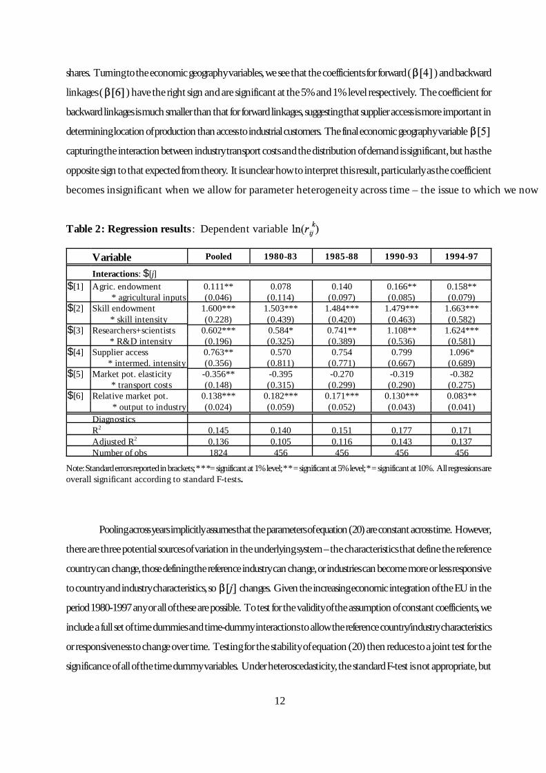
shares. Turningtotheeconomicgeographyvariables,weseethatthecoefficientsforforward( )andbackward

linkages( )havetherightsignandaresignificantatthe5%and1%levelrespectively. Thecoefficientfor

backwardlinkagesismuchsmallerthanthatforforwardlinkages,suggestingthatsupplieraccessismoreimportantin

determininglocationofproductionthanaccesstoindustrialcustomers. Thefinaleconomicgeographyvariable

capturingtheinteractionbetweenindustrytransportcostsandthedistributionofdemandissignificant,buthasthe

oppositesigntothatexpectedfromtheory. Itisunclearhowtointerpretthisresult,particularlyasthecoefficient

becomes insignificant when we allow for parameter heterogeneity across time – the issue to which we now

Table 2: Regression results : Dependent variable

Variable Pooled 1980-83 1985-88 1990-93 1994-97

Interactions: $[j]$[1] Agric. endowment 0.111** 0.078 0.140 0.166** 0.158**

* agricultural inputs (0.046) (0.114) (0.097) (0.085) (0.079)$[2] Skill endowment 1.600*** 1.503*** 1.484*** 1.479*** 1.663***

* skill intensity (0.228) (0.439) (0.420) (0.463) (0.582)$[3] Researchers+scientists 0.602*** 0.584* 0.741** 1.108** 1.624***

* R&D intensity (0.196) (0.325) (0.389) (0.536) (0.581)$[4] Supplier access 0.763** 0.570 0.754 0.799 1.096*

* intermed. intensity (0.356) (0.811) (0.771) (0.667) (0.689)$[5] Market pot. elasticity -0.356** -0.395 -0.270 -0.319 -0.382

* transport costs (0.148) (0.315) (0.299) (0.290) (0.275)$[6] Relative market pot. 0.138*** 0.182*** 0.171*** 0.130*** 0.083**

* output to industry (0.024) (0.059) (0.052) (0.043) (0.041)DiagnosticsR2 0.145 0.140 0.151 0.177 0.171Adjusted R2 0.136 0.105 0.116 0.143 0.137Number of obs 1824 456 456 456 456

Note:Standarderrorsreportedinbrackets;***=significantat1%level;**=significantat5%level;*=significantat10%. Allregressionsareoverall significant according to standard F-tests.

Poolingacrossyearsimplicitlyassumesthattheparametersofequation(20)areconstantacrosstime. However,

therearethreepotentialsourcesofvariationintheunderlyingsystem–thecharacteristicsthatdefinethereference

countrycanchange,thosedefiningthereferenceindustrycanchange,orindustriescanbecomemoreorlessresponsive

tocountryandindustrycharacteristics,so changes. GiventheincreasingeconomicintegrationoftheEUinthe

period1980-1997anyorallofthesearepossible. Totestforthevalidityoftheassumptionofconstantcoefficients,we

includeafullsetoftimedummiesandtime-dummyinteractionstoallowthereferencecountry/industrycharacteristics

orresponsivenesstochangeovertime. Testingforthestabilityofequation(20)thenreducestoajointtestforthe

significanceofallofthetimedummyvariables. Underheteroscedasticity,thestandardF-testisnotappropriate,but

13

(21)

(22)

calculationoftheappropriateWhiteheteroscedasticconsistentcovariancematrixallowsustotestforsignificanceusing

aWaldtest. Theassumptionofconstantparametersacrosstimeinvolvesimposing57restrictions,producingaWald

statisticof2003,whichisclearlysignificant(theWaldtestisdistributedChi-squaredwith57degreesoffreedom),leading

torejectionofthehypothesisthatparametersareconstant. Giventhattheparametersvaryovertimeinallthree

dimensions,wesplitthesampleandestimateseparatelyforeachoffourperiods,1980-83,1985-8,1990-93and1994-97.

Separatingtheyearsalsoreducesthedegreeofendogeneityofsomeoftheexplanatoryvariables.18 Theseestimatesare

given in remaining columns of Table 2.

Fromthefirstthreerows,weseethatthecomparativeadvantagevariableshavethesamesignsaspredictedby

theoryandthatthecoefficientsaremostlysignificantandincreasinginmagnitudeaswemovetolatertimeperiods. By

thefinalperiod,agriculture,skills,andR&Daresignificantatthe5%,1%and1%levelsrespectively. Aswiththepooled

results,thecoefficientsforagricultureareconsistentlysmallerthanforskillandR&Dintensity. Skillintensityisinitially

more important than R&D, although the two factors are equally important by the final period.

Resultsfortheeconomicgeographyvariablesaremoremixed. Backwardlinkages( )arealwayssignificant

atthe5%level(indeedatthe1%levelforthefirstthreeperiods). Forwardlinkages aresignificantatthe10%

level,butonlyforthelastperiod. Changesinthecoefficientssuggestthatthebackwardlinkagehasbecomelessstrong

throughtime,whiletheforwardlinkagehasbecomestronger. Thissaysthatsectorshighlyintensiveinintermediate

goodsaremovingtowardscentrallocationstogetbetteraccesstothesegoods,whileaccesstoindustrialcustomershas

decreasedinimportance. Thetransportcostcoefficient, isinsignificantinallsub-periodssuggestingthatthe

interaction between market potential and transport costs has no significant impact on the location of indu

Sofar,wehaveconcentratedonthedirectestimatesofthecoefficientsontheinteractionterms. However,we

canalsocalculateindustryspecificRybczynskieffectsandcountryspecificHeckscher-Ohlineffects. Fromequation(20)

the Rybczynski effects are

while the Heckscher-Ohlin effects take the form

14

Tocalculatetheseweneed,inadditiontotheinteractioncoefficients ,theleveleffects and ,given

in appendix table A2, and industry and country characteristics and , from appendix A5.20

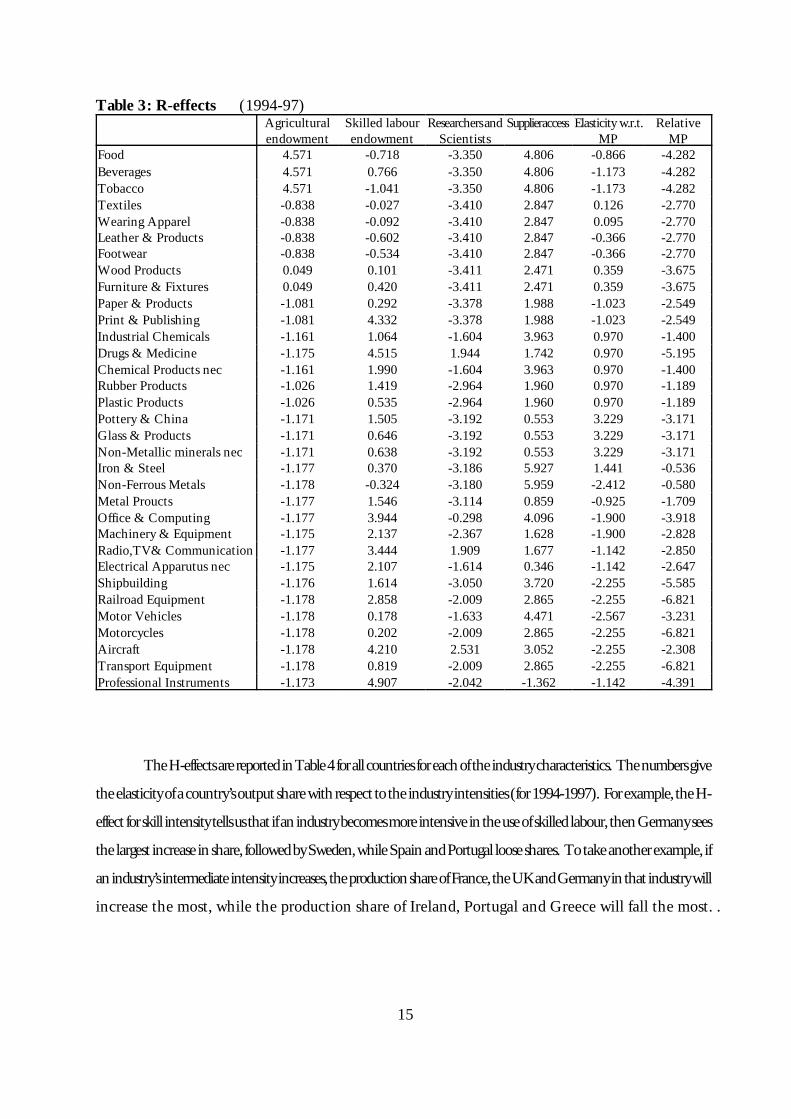
Table3reportsR-effectsforallindustriesforeachofthesixcountrycharacteristics. Thenumbersgiveninthe

tablearetheelasticityofeachindustry’soutputsharewithrespecttothecorrespondingcountrycharacteristic(for1994-

1997). ThesizeoftheR-effectdependsonthevalueoftheindustrycharacteristicrelativetoitsestimatedreference

value,andonthestrengthoftherelevantinteractionascapturedby$. Lookingat,forexample,skilledlabour,wesee

positiveR-effectsfor26ofthe33industries,withthelargestpositiveeffectsoccurringinProfessionalInstruments,

followedbyDrugsandMedicines,andPrintingandPublishing. Fortheresearchersandscientists,onlythreeindustries

havepositiveR-effects–Aircraft,DrugsandMedicines,andRadio,TVandCommunicationsequipment.21 Asafinal

example,weseethatsupplieraccesshasapositiveeffectonallbutoneindustry(Professionalinstruments),andtheeffects

are especially strong for Iron and Steel and for Non-ferrous metals.

NotethatwearecalculatingmarginalR-effectswithrespecttochangesinonecountrycharacteristicatatime.

Insomecases,whenthereferenceintensityisoutsidetherangeofobservedintensities,allofthemarginaleffectswillbe

ofonesign. Initiallythiswouldseeminconsistentwithouruseofadouble-relativemeasureofproductionshares.

However,itpurelyreflectsthefactthatwhenthereiscorrelationacrossthecountrycharacteristicsanygivenmarginal

R-effectcanbemorethanoffsetbytheR-effectsfromothercharacteristics. WeseeanexampleofthisinTable3for

relativemarketpotentialwherealloftheR-effectsarenegative. Insuchcases,the rankingandmagnitudeoftheeffects

are still informative.

15

Table 3: R-effects (1994-97)Agriculturalendowment

Skilled labourendowment

ResearchersandScientists

Supplieraccess Elasticity w.r.t.MP

RelativeMP

Food 4.571 -0.718 -3.350 4.806 -0.866 -4.282Beverages 4.571 0.766 -3.350 4.806 -1.173 -4.282Tobacco 4.571 -1.041 -3.350 4.806 -1.173 -4.282Textiles -0.838 -0.027 -3.410 2.847 0.126 -2.770Wearing Apparel -0.838 -0.092 -3.410 2.847 0.095 -2.770Leather & Products -0.838 -0.602 -3.410 2.847 -0.366 -2.770Footwear -0.838 -0.534 -3.410 2.847 -0.366 -2.770Wood Products 0.049 0.101 -3.411 2.471 0.359 -3.675Furniture & Fixtures 0.049 0.420 -3.411 2.471 0.359 -3.675Paper & Products -1.081 0.292 -3.378 1.988 -1.023 -2.549Print & Publishing -1.081 4.332 -3.378 1.988 -1.023 -2.549Industrial Chemicals -1.161 1.064 -1.604 3.963 0.970 -1.400Drugs & Medicine -1.175 4.515 1.944 1.742 0.970 -5.195Chemical Products nec -1.161 1.990 -1.604 3.963 0.970 -1.400Rubber Products -1.026 1.419 -2.964 1.960 0.970 -1.189Plastic Products -1.026 0.535 -2.964 1.960 0.970 -1.189Pottery & China -1.171 1.505 -3.192 0.553 3.229 -3.171Glass & Products -1.171 0.646 -3.192 0.553 3.229 -3.171Non-Metallic minerals nec -1.171 0.638 -3.192 0.553 3.229 -3.171Iron & Steel -1.177 0.370 -3.186 5.927 1.441 -0.536Non-Ferrous Metals -1.178 -0.324 -3.180 5.959 -2.412 -0.580Metal Proucts -1.177 1.546 -3.114 0.859 -0.925 -1.709Office & Computing -1.177 3.944 -0.298 4.096 -1.900 -3.918Machinery & Equipment -1.175 2.137 -2.367 1.628 -1.900 -2.828Radio,TV& Communication -1.177 3.444 1.909 1.677 -1.142 -2.850Electrical Apparutus nec -1.175 2.107 -1.614 0.346 -1.142 -2.647Shipbuilding -1.176 1.614 -3.050 3.720 -2.255 -5.585Railroad Equipment -1.178 2.858 -2.009 2.865 -2.255 -6.821Motor Vehicles -1.178 0.178 -1.633 4.471 -2.567 -3.231Motorcycles -1.178 0.202 -2.009 2.865 -2.255 -6.821Aircraft -1.178 4.210 2.531 3.052 -2.255 -2.308Transport Equipment -1.178 0.819 -2.009 2.865 -2.255 -6.821Professional Instruments -1.173 4.907 -2.042 -1.362 -1.142 -4.391

TheH-effectsarereportedinTable4forallcountriesforeachoftheindustrycharacteristics. Thenumbersgive

theelasticityofacountry’soutputsharewithrespecttotheindustryintensities(for1994-1997). Forexample,theH-

effectforskillintensitytellsusthatifanindustrybecomesmoreintensiveintheuseofskilledlabour,thenGermanysees

thelargestincreaseinshare,followedbySweden,whileSpainandPortugallooseshares. Totakeanotherexample,if

anindustry’sintermediateintensityincreases,theproductionshareofFrance,theUKandGermanyinthatindustrywill

increase the most, while the production share of Ireland, Portugal and Greece will fall the most. .

16

Table 4: H-effects (1994-97)Agricultural

intensitySkill

intensityR&D

intensityIntermediate

intensityTransportintensity Shareofoutput to

industryAustria 0.146 2.763 -0.956 -0.641 0.863 0.022Belgium 0.086 1.764 -0.015 -0.514 0.823 0.039Denmark 0.543 3.179 -0.411 -1.219 0.901 0.043Spain 0.284 -0.782 -2.939 0.155 0.675 0.005Finland 0.366 2.606 1.074 -1.380 0.933 0.027France 0.239 1.923 -0.194 1.064 0.231 -0.090UK 0.132 1.337 -1.045 0.800 0.365 0.014Germany 0.048 3.179 -0.411 1.430 -0.371 0.288Greece 0.522 0.802 -2.205 -1.634 0.945 0.008Ireland 0.487 0.987 1.496 -1.929 0.948 0.038Italy 0.270 -0.012 -2.805 0.868 0.399 -0.057Netherlands 0.291 2.154 -1.494 -0.272 0.773 0.020Portugal 0.342 -2.593 -3.812 -1.439 0.923 0.039Sweden 0.192 2.862 1.228 -0.736 0.873 0.015

5.3 Robustness

Beforeconsideringtheoverallfitandtherelativeimportanceofcomparativeadvantagevariablestoeconomicgeography

variables,webrieflyconsidertherobustnessofourresults. InestimatingthecoefficientsinTable2,ourspecificationofthe

errorstructureallowedforthepossibilityofheteroscedasticityduetodifferencesacrossindustriesorcountries,butignored

thefactthatwehaveanindustry-countrypanelforeachoftheyears. Thatis,weignoredthepossibilitythatshocksmight

becorrelatedacrossindustriesand/orcountries. Therearetwopossiblesourcesforsuchcountry/industryspecificshocks.

First,aparticularindustryorcountrymightexperienceashocktoitsshareinEuropeanwideproduction. Lookingbackto

equation(10)itisclearthatouruseofthedoublerelativemeasuremeansthatourspecificationisrobusttosuchshocks.

However,itispossiblethatcountryorindustrycharacteristicsmightbeconsistentlymismeasuredforoneparticularcountry

orindustry. Again,fromequation(10)itisclearthatthesemeasurementerrorswouldtranslateintofixedeffectsforthe

countryorindustryconcerned. Totesttherobustnessofourresultstothisformofspecificationerror,weincludeafullset

ofcountrydummiesandindustrydummiesandre-estimateequation(20),droppingthe12countryandindustrylevels

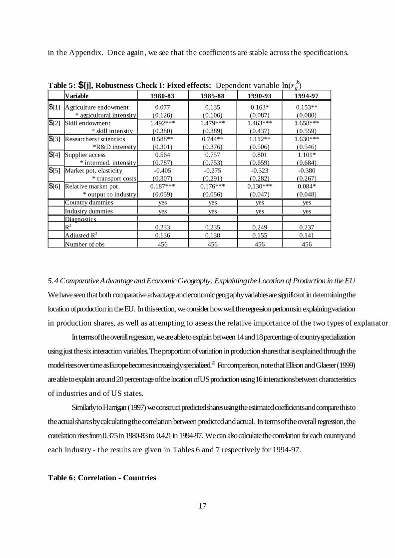
variables. TheresultsfortheinteractionvariablesforeachoftheyearsarereportedinTable5. Theyindicatethatour

resultsontheinteractiontermsarerobusttotheinclusionofindustryandcountryfixedeffects. Theexplanatorypowerof

theequationisincreased,aswouldbeexpected,withR2risingfromaround17%to24%,whilethechangesintheestimates

of $[j] are negligible.

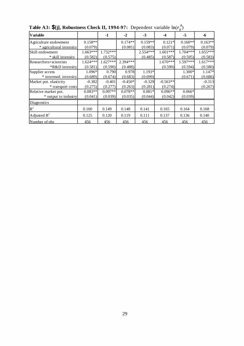
Wealsotesttherobustnessofourspecificationbydroppingeachoftheinteractionsinturnfromtheestimating

equation. Weundertakethisjustforthe1994-97dataset,andreportonlytheinteractioncoefficients,$[j],inTableA3

17

in the Appendix. Once again, we see that the coefficients are stable across the specifications.

Table 5: $$$$[j], Robustness Check I: Fixed effects: Dependent variableVariable 1980-83 1985-88 1990-93 1994-97

$[1] Agriculture endowment 0.077 0.135 0.163* 0.153*** agricultural intensity (0.126) (0.106) (0.087) (0.080)

$[2] Skill endowment 1.492*** 1.479*** 1.463*** 1.658**** skill intensity (0.380) (0.389) (0.437) (0.559)

$[3] Researchers+scientists 0.588** 0.744** 1.112** 1.630****R&D intensity (0.301) (0.376) (0.506) (0.546)

$[4] Supplier access 0.564 0.757 0.801 1.101** intermed. intensity (0.787) (0.753) (0.659) (0.684)

$[5] Market pot. elasticity -0.405 -0.275 -0.323 -0.380* transport costs (0.307) (0.291) (0.282) (0.267)

$[6] Relative market pot. 0.187*** 0.176*** 0.130*** 0.084** output to industry (0.059) (0.056) (0.047) (0.048)

Country dummies yes yes yes yesIndustry dummies yes yes yes yesDiagnosticsR2 0.233 0.235 0.249 0.237Adjusted R2 0.136 0.138 0.155 0.141Number of obs 456 456 456 456

5.4 Comparative Advantage and Economic Geography: Explaining the Location of Production in the EU

Wehaveseenthatbothcomparativeadvantageandeconomicgeographyvariablesaresignificantindeterminingthe

locationofproductionintheEU. Inthissection,weconsiderhowwelltheregressionperformsinexplainingvariation

in production shares, as well as attempting to assess the relative importance of the two types of explanator

Intermsoftheoverallregression,weareabletoexplainbetween14and18percentageofcountryspecialization

usingjustthesixinteractionvariables.Theproportionofvariationinproductionsharesthatisexplainedthroughthe

modelrisesovertimeasEuropebecomesincreasinglyspecialized.22 Forcomparison,notethatEllisonandGlaeser(1999)

areabletoexplainaround20percentageofthelocationofUSproductionusing16interactionsbetweencharacteristics

of industries and of US states.

SimilarlytoHarrigan(1997)weconstructpredictedsharesusingtheestimatedcoefficientsandcomparethisto

theactualsharesbycalculatingthecorrelationbetweenpredictedandactual. Intermsoftheoverallregression,the

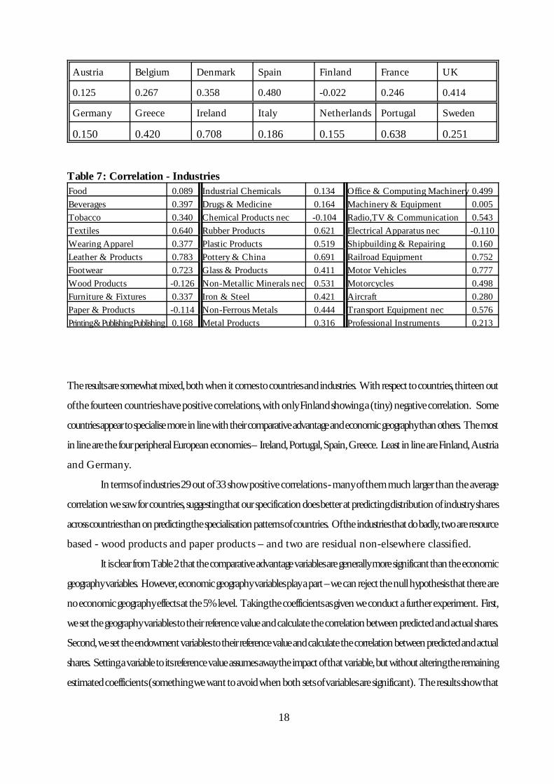
correlationrisesfrom0.375in1980-83to 0.421in1994-97. Wecanalsocalculatethecorrelationforeachcountryand

each industry - the results are given in Tables 6 and 7 respectively for 1994-97.

Table 6: Correlation - Countries

18

Austria Belgium Denmark Spain Finland France UK

0.125 0.267 0.358 0.480 -0.022 0.246 0.414

Germany Greece Ireland Italy Netherlands Portugal Sweden

0.150 0.420 0.708 0.186 0.155 0.638 0.251

Table 7: Correlation - IndustriesFood 0.089 Industrial Chemicals 0.134 Office & Computing Machinery 0.499Beverages 0.397 Drugs & Medicine 0.164 Machinery & Equipment 0.005Tobacco 0.340 Chemical Products nec -0.104 Radio,TV & Communication 0.543Textiles 0.640 Rubber Products 0.621 Electrical Apparatus nec -0.110Wearing Apparel 0.377 Plastic Products 0.519 Shipbuilding & Repairing 0.160Leather & Products 0.783 Pottery & China 0.691 Railroad Equipment 0.752Footwear 0.723 Glass & Products 0.411 Motor Vehicles 0.777Wood Products -0.126 Non-Metallic Minerals nec 0.531 Motorcycles 0.498Furniture & Fixtures 0.337 Iron & Steel 0.421 Aircraft 0.280Paper & Products -0.114 Non-Ferrous Metals 0.444 Transport Equipment nec 0.576Printing&PublishingPublishing 0.168 Metal Products 0.316 Professional Instruments 0.213

Theresultsaresomewhatmixed,bothwhenitcomestocountriesandindustries. Withrespecttocountries,thirteenout

ofthefourteencountrieshavepositivecorrelations,withonlyFinlandshowinga(tiny)negativecorrelation. Some

countriesappeartospecialisemoreinlinewiththeircomparativeadvantageandeconomicgeographythanothers. Themost

inlinearethefourperipheralEuropeaneconomies– Ireland,Portugal,Spain,Greece. LeastinlineareFinland,Austria

and Germany.

Intermsofindustries29outof33showpositivecorrelations-manyofthemmuchlargerthantheaverage

correlationwesawforcountries,suggestingthatourspecificationdoesbetteratpredictingdistributionofindustryshares

acrosscountriesthanonpredictingthespecialisationpatternsofcountries. Oftheindustriesthatdobadly,twoareresource

based - wood products and paper products – and two are residual non-elsewhere classified.

ItisclearfromTable2thatthecomparativeadvantagevariablesaregenerallymoresignificantthantheeconomic

geographyvariables. However,economicgeographyvariablesplayapart–wecanrejectthenullhypothesisthatthereare

noeconomicgeographyeffectsatthe5%level. Takingthecoefficientsasgivenweconductafurtherexperiment. First,

wesetthegeographyvariablestotheirreferencevalueandcalculatethecorrelationbetweenpredictedandactualshares.

Second,wesettheendowmentvariablestotheirreferencevalueandcalculatethecorrelationbetweenpredictedandactual

shares. Settingavariabletoitsreferencevalueassumesawaytheimpactofthatvariable,butwithoutalteringtheremaining

estimatedcoefficients(somethingwewanttoavoidwhenbothsetsofvariablesaresignificant). Theresultsshowthat

19

disregardingtheimpactofeconomicgeographyvariablesreducesthecorrelationbetweenpredictedandactualsharesby

approximately13%,whiledisregardingtheimpactofcomparativeadvantagevariablesreducesthecorrelationbetween

predicted and actual shares by approximately 44%, again confirming that economic geography does matte

7. Concluding comments

Thetheoreticalmodeldevelopedinthispaperprovidesarigorousframeworkinwhichcomparativeadvantagecanbe

combinedwithtransportcostsandgeography,toprovideamoregeneraltheoryoftradeandlocation. Resultsofthe

theoryareintuitive,andenableHeckscher-Ohlininsightstobegeneralisedtoenvironmentswithmoretradefrictions

thaniscommoninsuchmodels. Linearizationofthemodelprovidesanestimatingequationinwhichcountry

characteristics,industrycharacteristics,andmostimportantlytheinteractionofthetwo,combinetodeterminetheshares

of each industry in each country.

ImplementingthisequationonEUdata,wefindthatasubstantialpartoftheEU’scross-countryvariationin

industrial structurecanbeexplainedbytheforcescapturedinthemodel. Factorendowmentsareimportant. In

particular,countries’endowmentsofhighlyskilledlabourareimportantinattractinghighskill intensiveindustries.

Geographyalsomatters, as industriesdependentonforwardandbackwardlinkages locateclosetocentresof

manufacturingsupplyanddemand. EconomicintegrationandfallinglevelsofnationalgovernmentinterventioninEU

industrysuggeststhateconomicforcesshouldhavebecomeincreasinglyimportantindeterminingindustriallocation,

and we find some evidence that this is so.

Ourapproachisbasedonindustriesthatareperfectlycompetitive,andtheomissionofimperfectcompetition

isimportant. However,toincludeimperfectcompetitionwouldcreatesignificantcomplexitiesthatwehavesoughtto

avoidatthisstage. Forexample,theorysuggeststhatinsuchanenvironment,itisgenerallyindustrieswithintermediate

levelsoftransportcoststhataredrawnintocentrallocations,creatinganon-monotonicrelationshipbetweentransport

intensityandlocation(thisperhapsaccountingforthepoorperformanceofourtransportintensityvariable). General

casesinwhichtherearemanyindustries,someperfectlyandothersimperfectlycompetitive,andallsubjecttotransport

costshaveyettobeworkedout. Andweknowthatinsuchenvironmentsintermediategoodscreateamultiplicityof

equilibria, as agglomerations may form. All of these issues are the subject of our ongoing research.

20

(23)

(24)

(25)

(26)

(27)

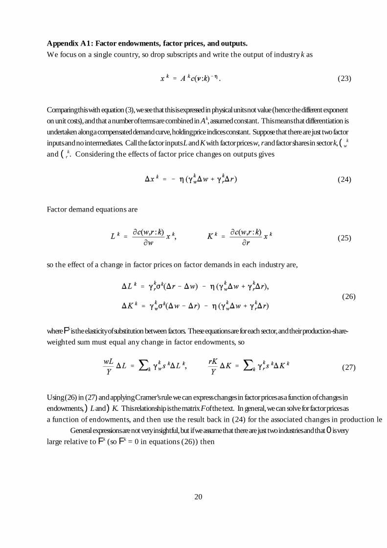
Appendix A1: Factor endowments, factor prices, and outputs.We focus on a single country, so drop subscripts and write the output of industry k as

Comparingthiswithequation(3),weseethatthisisexpressedinphysicalunitsnotvalue(hencethedifferentexponentonunitcosts),andthatanumberoftermsarecombinedinAk,assumedconstant. Thismeansthatdifferentiationisundertakenalongacompensateddemandcurve,holdingpriceindicesconstant. Supposethattherearejusttwofactorinputsandnointermediates. CallthefactorinputsLandKwithfactorpricesw,randfactorsharesinsectork,(w

k

and (rk. Considering the effects of factor price changes on outputs gives

Factor demand equations are

so the effect of a change in factor prices on factor demands in each industry are,

whereFkistheelasticityofsubstitutionbetweenfactors. Theseequationsareforeachsector,andtheirproduction-share-weighted sum must equal any change in factor endowments, so

Using(26)in(27)andapplyingCramer’srulewecanexpresschangesinfactorpricesasafunctionofchangesinendowments,)Land)K. ThisrelationshipisthematrixFofthetext. Ingeneral,wecansolveforfactorpricesasa function of endowments, and then use the result back in (24) for the associated changes in production le

Generalexpressionsarenotveryinsightful,butifweassumethattherearejusttwoindustriesandthat0isverylarge relative to Fk (so Fk = 0 in equations (26)) then

21

(28)

(29)

(30)

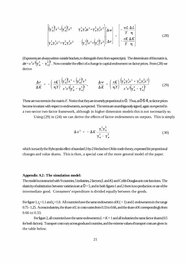
(Exponentsarealwayswrittenoutsidebrackets,todistinguishthemfromsuperscripts). Thedeterminantofthismatrixis,det= . Nowconsidertheeffectofachangeincapitalendowmentonfactorprices. From(28)wederive

ThesearetwotermsinthematrixF. Noticethattheyareinverselyproportionalto0. Thus,as064,sofactorpricesbecomeinvariantwithrespecttoendowments,asexpected. Thetermsareunambiguouslysigned,againasexpectedina two-sector two-factor framework, although in higher dimension models this is not necessarily so.

Using (29) in (24) we can derive the effects of factor endowments on outputs. This is simply

whichisexactlytheRybczynskieffectofstandard2-by-2Heckscher-Ohlintradetheory,expressedforproportionalchanges and value shares. This is then, a special case of the more general model of the paper.

Appendix A2: The simulation model:Themodelisconstructedwith9countries,5industries,2factors(LandK)andCobb-Douglasunitcostfunctions. Theelasticityofsubstitutionbetweenvarietiesissetat0=5,andinbothfigures1and2thereisnoproductionoruseoftheintermediate good. Consumers’ expenditure is divided equally between the goods.

Forfigure1, tij=1.1and tii=1.0. AllcountrieshavethesameendowmentofK(=1)andLendowmentsintherange0.75-1.25. Acrossindustries,theshareofL incostsvariesfrom0.33to0.66,andtheshareofKcorrespondinglyfrom0.66 to 0.33.

Forfigure2,allcountrieshavethesameendowmentsL=K=1andallindustriesthesamefactorshares(0.5forbothfactors). Transportcostsvaryacrossgoodsandcountries,andtheextremevaluesoftransportcostsaregiveninthe table below.

22

(31)

Least transportintensive good

Most transport intensivegood

2 closest economies 1.003 1.03

2 furthest economies 1.045 1.49

Thehorizontalaxesmeasurethetransportcostsbetweenthetwoclosesteconomiesfordifferentindustries,2k,andthemarket potential of different countries, computed from equation (9) for the middle ranked industry.

Appendix A3: Construction of variables1)Dependentvariable: : logof industryoutputlevels,expressedrelativetoboththeEUoutputof industrykasawhole,andtothetotalmanufacturingoutputofcountry i. Thisvalueiscalculatedfromtheproductiondataforeach of the 36 sectors (see Appendix A4).

2)Primaryfactors: Weusethreefactorintensity/ factorendowmentinteractions, forskilledlabour, researchersand scientists, and agricultureA) Share of factors in costs of each industry, (w :

i)Skilledlabourintensity: proxiedbytheproportionofnon-manualworkersinthesector’semploymenttimeslabour compensation as % gross output.ii)R&Dintensity: R&Dexpenditureas%grossoutput. Thisincludessomenon-labourcomponents,althoughthe major share of R&D expenditure is personnel costs.iii) Agricultural intensity: Inputs from agriculture, fishery and forestry as % gross output.

B) Endowments, ))))L i:i) Skilled labour: proportion of the population with secondary education or higher (logs).ii) Researchers and scientists per ten thousand labour force (logs).iii)Agriculturalabundance:proxiedbygrossvalueaddedofagriculture,forestryandfisheryproductsas%ofall branches (logs).

3) Intermediate supply: Forward linkagesA) Share of intermediate in costs of each industry, (q: from input-output tables.B) Priceoftheintermediategood,)qi:Theintermediatepriceineachcountryisgivenbyequation(6),andisafunction of price indices Gi

k, as defined in equation (2). Using (3) with equation (2) gives:

23

(32)

(33)

(34)

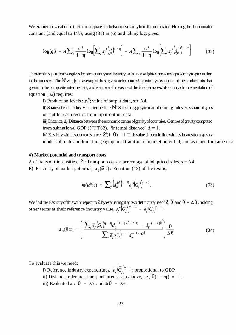
Weassumethatvariationintheterminsquarebracketscomesmainlyfromthenumerator. Holdingthedenominatorconstant (and equal to 1/A), using (31) in (6) and taking logs gives,

Theterminsquarebracketsgives,foreachcountryandindustry,adistanceweightedmeasureofproximitytoproductionintheindustry. TheNkweightedaverageofthesegiveseachcountry’sproximitytosuppliersoftheproductmixthatgoesintothecompositeintermediate,andisanoverallmeasureofthe‘supplieraccess’ofcountry i.Implementationofequation (32) requires:

i) Production levels : ; value of output data, see A4.ii)Sharesofeachindustryinintermediate,Nk:Salestoaggregatemanufacturingindustryasshareofgrossoutput for each sector, from input-output data.iii)Distance,dij: Distancebetweentheeconomiccentreofgravityofcountries. Centresofgravitycomputedfrom subnational GDP (NUTS2). ‘Internal distance’, dii = 1.iv)Elasticitywithrespecttodistance: 2k(1-0)=-1. Thisvaluechoseninlinewithestimatesfromgravitymodels of trade and from the geographical tradition of market potential, and assumed the same in a

4) Market potential and transport costsA) Transport intensities, 2k: Transport costs as percentage of fob priced sales, see A4.B) Elasticity of market potential, : Equation (18) of the text is,

Wefindtheelasticityofthiswithrespectto2byevaluatingitattwodistinctvaluesof2, and ,holdingother terms at their reference industry value, :

To evaluate this we need:i) Reference industry expenditures, ; proportional to GDPj.ii) Distance, reference transport intensity, as above, i.e., .iii) Evaluated at: and .

24

(35)

(36)

(37)

(38)

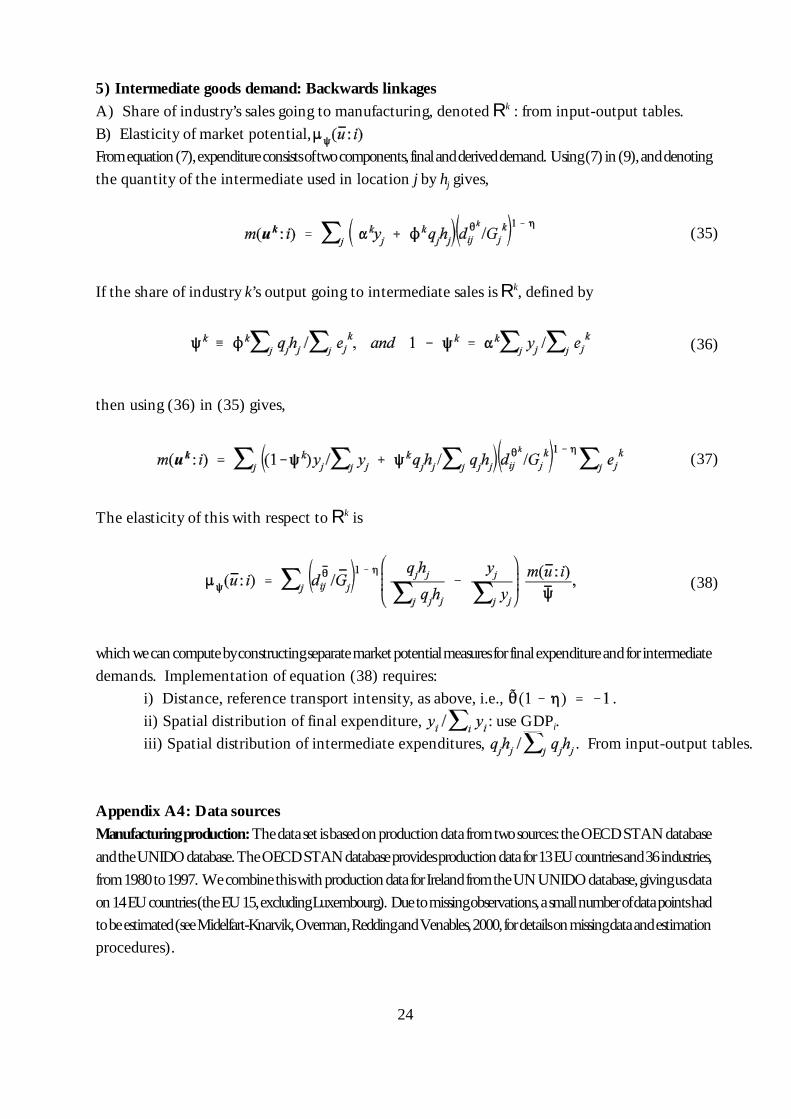
5) Intermediate goods demand: Backwards linkagesA) Share of industry’s sales going to manufacturing, denoted Rk : from input-output tables.B) Elasticity of market potential,Fromequation(7),expenditureconsistsoftwocomponents,finalandderiveddemand. Using(7)in(9),anddenotingthe quantity of the intermediate used in location j by hj gives,

If the share of industry k’s output going to intermediate sales is Rk, defined by

then using (36) in (35) gives,

The elasticity of this with respect to Rk is

whichwecancomputebyconstructingseparatemarketpotentialmeasuresforfinalexpenditureandforintermediatedemands. Implementation of equation (38) requires:

i) Distance, reference transport intensity, as above, i.e., .ii) Spatial distribution of final expenditure, : use GDPi.iii) Spatial distribution of intermediate expenditures, . From input-output tables.

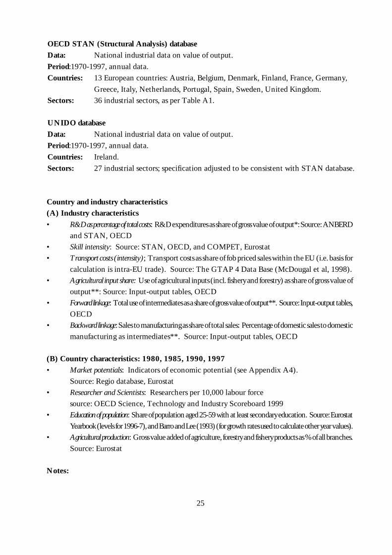
Appendix A4: Data sourcesManufacturingproduction:Thedatasetisbasedonproductiondatafromtwosources:theOECDSTANdatabaseandtheUNIDOdatabase.TheOECDSTANdatabaseprovidesproductiondatafor13EUcountriesand36industries,from1980to1997. WecombinethiswithproductiondataforIrelandfromtheUNUNIDOdatabase,givingusdataon14EUcountries(theEU15,excludingLuxembourg). Duetomissingobservations,asmallnumberofdatapointshadtobeestimated(seeMidelfart-Knarvik,Overman,ReddingandVenables,2000,fordetailsonmissingdataandestimationprocedures).

25

OECD STAN (Structural Analysis) databaseData: National industrial data on value of output.Period:1970-1997, annual data.Countries: 13 European countries: Austria, Belgium, Denmark, Finland, France, Germany,

Greece, Italy, Netherlands, Portugal, Spain, Sweden, United Kingdom.Sectors: 36 industrial sectors, as per Table A1.

UNIDO databaseData: National industrial data on value of output.Period:1970-1997, annual data.Countries: Ireland.Sectors: 27 industrial sectors; specification adjusted to be consistent with STAN database.

Country and industry characteristics(A) Industry characteristics• R&Daspercentageoftotalcosts: R&Dexpendituresasshareofgrossvalueofoutput*:Source:ANBERD

and STAN, OECD• Skill intensity: Source: STAN, OECD, and COMPET, Eurostat• Transport costs (intensity); Transport costs as share of fob priced sales within the EU (i.e. basis for

calculation is intra-EU trade). Source: The GTAP 4 Data Base (McDougal et al, 1998).• Agricultural input share: Useofagricultural inputs(incl. fisheryandforestry)as shareof grossvalueof

output**: Source: Input-output tables, OECD• Forwardlinkage: Totaluseofintermediatesasashareofgrossvalueofoutput**. Source:Input-outputtables,

OECD• Backwardlinkage:Salestomanufacturingasshareoftotal sales: Percentageofdomesticsalestodomestic

manufacturing as intermediates**. Source: Input-output tables, OECD

(B) Country characteristics: 1980, 1985, 1990, 1997• Market potentials: Indicators of economic potential (see Appendix A4).

Source: Regio database, Eurostat• Researcher and Scientists: Researchers per 10,000 labour force

source: OECD Science, Technology and Industry Scoreboard 1999• Educationofpopulation: Shareofpopulationaged25-59withatleastsecondaryeducation. Source:Eurostat

Yearbook(levelsfor1996-7),andBarroandLee(1993)(forgrowthratesusedtocalculateotheryearvalues).• Agriculturalproduction: Grossvalueaddedofagriculture,forestryandfisheryproductsas%ofallbranches.

Source: Eurostat

Notes:

26

*)AsindustryintensitiesareassumedtobeequalacrosscountriesR&Dsharesofgrossvalueofoutputarecalculatedasweightedaverages.WeusedataforDenmark,Finland,France,Germany(formerFRG),Italy,Netherlands,Spain,Swedenand the UK for the year 1990.**)Weuseaweightedaverageof1990IOtablesforDenmark,France,GermanyandtheUKtocalculateintermediateinputsharesandthe destinationof finaloutput(intermediateusagevsfinalusage). Intermediatesincludebothdomesticallypurchasedandimportedinputs. Thedataneededtocalculatetheindustryintensitieswereingeneralnotavailableforthe36sectorsdisaggregation,sointensitiescalculatedatacruderlevelofdisaggregation,weremappedintothe 36 sectors classification.

27

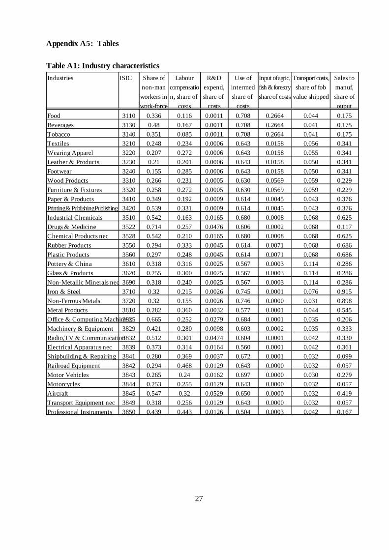
Appendix A5: Tables

Table A1: Industry characteristics

Industries ISIC Share ofnon-manworkers inwork-force

Labourcompensation, share of

costs

R&Dexpend,share of

costs

Use ofintermedshare of

costs

Inputofagric,fish&forestryshareof costs

Transportcosts,share of fob

value shipped

Sales tomanuf,share ofouput

Food 3110 0.336 0.116 0.0011 0.708 0.2664 0.044 0.175Beverages 3130 0.48 0.167 0.0011 0.708 0.2664 0.041 0.175Tobacco 3140 0.351 0.085 0.0011 0.708 0.2664 0.041 0.175Textiles 3210 0.248 0.234 0.0006 0.643 0.0158 0.056 0.341Wearing Apparel 3220 0.207 0.272 0.0006 0.643 0.0158 0.055 0.341Leather & Products 3230 0.21 0.201 0.0006 0.643 0.0158 0.050 0.341Footwear 3240 0.155 0.285 0.0006 0.643 0.0158 0.050 0.341Wood Products 3310 0.266 0.231 0.0005 0.630 0.0569 0.059 0.229Furniture & Fixtures 3320 0.258 0.272 0.0005 0.630 0.0569 0.059 0.229Paper & Products 3410 0.349 0.192 0.0009 0.614 0.0045 0.043 0.376Printing&PublishingPublishing 3420 0.539 0.331 0.0009 0.614 0.0045 0.043 0.376Industrial Chemicals 3510 0.542 0.163 0.0165 0.680 0.0008 0.068 0.625Drugs & Medicine 3522 0.714 0.257 0.0476 0.606 0.0002 0.068 0.117Chemical Products nec 3528 0.542 0.210 0.0165 0.680 0.0008 0.068 0.625Rubber Products 3550 0.294 0.333 0.0045 0.614 0.0071 0.068 0.686Plastic Products 3560 0.297 0.248 0.0045 0.614 0.0071 0.068 0.686Pottery & China 3610 0.318 0.316 0.0025 0.567 0.0003 0.114 0.286Glass & Products 3620 0.255 0.300 0.0025 0.567 0.0003 0.114 0.286Non-Metallic Minerals nec 3690 0.318 0.240 0.0025 0.567 0.0003 0.114 0.286Iron & Steel 3710 0.32 0.215 0.0026 0.745 0.0001 0.076 0.915Non-Ferrous Metals 3720 0.32 0.155 0.0026 0.746 0.0000 0.031 0.898Metal Products 3810 0.282 0.360 0.0032 0.577 0.0001 0.044 0.545Office & Computing Machinery3825 0.665 0.252 0.0279 0.684 0.0001 0.035 0.206Machinery & Equipment 3829 0.421 0.280 0.0098 0.603 0.0002 0.035 0.333Radio,TV & Communication3832 0.512 0.301 0.0474 0.604 0.0001 0.042 0.330Electrical Apparatus nec 3839 0.373 0.314 0.0164 0.560 0.0001 0.042 0.361Shipbuilding & Repairing 3841 0.280 0.369 0.0037 0.672 0.0001 0.032 0.099Railroad Equipment 3842 0.294 0.468 0.0129 0.643 0.0000 0.032 0.057Motor Vehicles 3843 0.265 0.24 0.0162 0.697 0.0000 0.030 0.279Motorcycles 3844 0.253 0.255 0.0129 0.643 0.0000 0.032 0.057Aircraft 3845 0.547 0.32 0.0529 0.650 0.0000 0.032 0.419Transport Equipment nec 3849 0.318 0.256 0.0129 0.643 0.0000 0.032 0.057Professional Instruments 3850 0.439 0.443 0.0126 0.504 0.0003 0.042 0.167

28

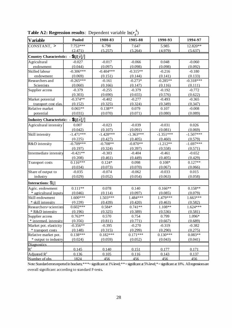
Table A2: Regression results : Dependent variable

Variable Pooled 1980-83 1985-88 1990-93 1994-97

CONSTANT, > 7.753*** 6.798 7.647 5.985 12.820**(2.471) (5.257) (5.264) (4.979) (5.637)

Country Characteristic: - $$$$[j]Agricultural -0.027 -0.017 -0.066 0.048 -0.060

endowment (0.044) (0.097) (0.098) (0.098) (0.092)Skilled labour -0.306*** -0.404*** -0.315** -0.216 -0.180

endowment (0.069) (0.151) (0.144) (0.141) (0.133)Researchers and -0.265*** -0.161 -0.273* -0.285** -0.318***

Scientists (0.060) (0.166) (0.147) (0.116) (0.111)Supplier access -0.379 -0.255 -0.379 -0.192 -0.772

(0.303) (0.690) (0.655) (0.576) (0.622)Market potential -0.374** -0.402 -0.277 -0.493 -0.365

transport cost elas. (0.152) (0.325) (0.324) (0.349) (0.347)Relative market 0.065** 0.138** 0.079 0.107 -0.008

potential (0.031) (0.070) (0.071) (0.080) (0.089)

Industry Characteristic: - $$$$[j]Agricultural intensity 0.007 -0.023 -0.039 -0.031 0.026

(0.042) (0.107) (0.091) (0.081) (0.069)Skill intensity -1.471*** -1.428*** -1.363*** -1.351*** -1.507***

(0.225) (0.427) (0.405) (0.460) (0.579)R&D intensity -0.709*** -0.708** -0.870** -1.212** -1.697***

(0.197) (0.324) (0.397) (0.558) (0.571)Intermediate intensity -0.421** -0.303 -0.404 -0.461 -0.652

(0.208) (0.461) (0.449) (0.405) (0.429)Transport costs 0.116*** 0.124* 0.098 0.108* 0.127**

(0.034) (0.073) (0.070) (0.067) (0.066)Share of output to -0.035 -0.074 -0.062 -0.033 0.015

industry (0.029) (0.052) (0.054) (0.063) (0.058)

Interactions: $[j]Agric. endowment 0.111** 0.078 0.140 0.166** 0.158**

* agricultural inputs (0.046) (0.114) (0.097) (0.085) (0.079)Skill endowment 1.600*** 1.503*** 1.484*** 1.479*** 1.663***

* skill intensity (0.228) (0.439) (0.420) (0.463) (0.582)Researchers+scientists 0.602*** 0.584* 0.741** 1.108** 1.624***

* R&D intensity (0.196) (0.325) (0.389) (0.536) (0.581)Supplier access 0.763** 0.570 0.754 0.799 1.096** intermed. intensity (0.356) (0.811) (0.771) (0.667) (0.689)

Market pot. elasticity -0.356** -0.395 -0.270 -0.319 -0.382* transport costs (0.148) (0.315) (0.299) (0.290) (0.275)

Relative market pot. 0.138*** 0.182*** 0.171*** 0.130*** 0.083*** output to industry (0.024) (0.059) (0.052) (0.043) (0.041)

DiagnosticsR2 0.145 0.140 0.151 0.177 0.171Adjusted R2 0.136 0.105 0.116 0.143 0.137Number of obs 1824 456 456 456 456Note:Standarderrorsreportedinbrackets;***=significantat1%level;**=significantat5%level;*=significantat10%. Allregressionsareoverall significant according to standard F-tests.

29

Table A3: $$$$[j], Robustness Check II, 1994-97: Dependent variable

Variable -1 -2 -3 -4 -5 -6

Agriculture endowment 0.158** 0.174** 0.159** 0.121* 0.160** 0.163*** agricultural intensity (0.079) (0.081) (0.083) (0.071) (0.079) (0.079)

Skill endowment 1.663*** 1.732*** 2.554*** 1.601*** 1.704*** 1.655**** skill intensity (0.582) (0.575) (0.485) (0.587) (0.595) (0.583)

Researchers+scientists 1.624*** 1.627*** 2.394*** 1.670*** 1.597*** 1.617****R&D intensity (0.581) (0.590) (0.488) (0.590) (0.594) (0.580)

Supplier access 1.096* 0.790 0.978 1.193* 1.300* 1.147** intermed. intensity (0.689) (0.674) (0.683) (0.699) (0.671) (0.686)

Market pot. elasticity -0.382 -0.401 -0.450* -0.329 -0.563** -0.313* transport costs (0.275) (0.277) (0.263) (0.281) (0.274) (0.267)

Relative market pot. 0.083** 0.097** 0.078** 0.081* 0.096** 0.066** output to industry (0.041) (0.039) (0.035) (0.044) (0.042) (0.039)

Diagnostics

R2 0.160 0.149 0.148 0.141 0.165 0.164 0.168

Adjusted R2 0.125 0.120 0.119 0.111 0.137 0.136 0.140

Number of obs 456 456 456 456 456 456 456

30

1.Unlikerecentworkbye.g.Trefler(1993,1995)theaimofthispaperisnottoprovideatestoftheHOVtheorem,buttoestimatehowfactorendowments,tradefrictionsandthegeographicaldistributionofdemandinteractindetermining the location of production and international specialization.

2. See Midelfart-Knarvik, Overman, Redding and Venables, (2000).

3. See Leamer and Levinsohn (1995) for a discussion and critique of this and other approaches.

4. See Fujita, Krugman and Venables (1999).

5. Lettingthiselasticitydifferacrossindustrieswouldbestraightforwardinthetheoreticalsections,butacommonvalue is assumed in the empirical estimation.

6. Havingmanyintermediategoodsandafull input-outputstructurewouldbeeasyintheory,butisdifficulttoimplementintheeconometrics. Thereasonisthatdiagonalelementsoftendominatetheinput-outputmatrix,sothatexamination of forward and backward linkages encounters severe endogeneity problems.

7. If therearenotransportcosts(all tijk =1)thenpriceindicesandmarketpotential takethesamevalueinall

locations, so production is determined by cost factors alone; otherwise, geography matters.

8. These properties both hold by appropriate choice of units.

9. Noticethat,atthereferencepoint,thereisnocross-industryvariationincosts(since forallk)orcross-countryvariationinmarketpotential(since forall i);thelinearisationcapturesthevariationin costs and industry characteristics away from the reference point.

10.WecaninprincipleestimatewiththefullmatrixF,notjustthediagonal,buttheresultingspecificationisbesetby multi-collinearity problems.

11.Endowmentsofotherfactorsarescaledbackequi-proportionatelytomaintaincountrysize,asaretheinputsharesof these factors

12. Local perturbation of the endowment in this direction has no effect on .

13.Sincewearefocussingonlyonthestructureofmanufacturing,wetakeagriculturalproductionasanexogenousmeasure of ‘agriculture abundance’, rather than going back to an underlying endowment such as land.

14. Thefigureonlyillustratestherangeinwhichthesaddleshapeholds. Increasingtransportintensityfurthercausesa flattening of the surface. As 2k 6 4 so the market potential of industry k becomes equal to local demand

15.Theresultingdatahastimevaryingcountrycharacteristics,whileindustryintensitiesareconstantacrossallfourtimeperiods. Thus,weareassumingthattherehavenotbeenmajorchangesinproductiontechnologiesgiventhelevel of aggregation of our industrial classification.

16.TheresultsonthesignificanceofcoefficientsarelargelyunchangedwhenwemovefromOLSstandarderrorstoheteroscedasticrobuststandarderrors. Thisreflectsthefactthatheteroscedasticityisunlikelytobeamajorproblemas we measuring shares (the left hand side variable) relative to industry and country size.

Endnotes:

31

17.Thisgivesusatotalof1824observations. Ineachofthefourtimeperiods,thereare6missingobservations:Denmark: ISIC 3842, 3845, 3849; France: ISIC 3849; Ireland: ISIC 3130; Netherlands: ISIC 3842.

18. Midelfart-Knarvik,Overman,ReddingandVenables(2000)showthattheindustrialproductionstructureofEuropechangesoverthistimeperiod. AssumingthatthisisinresponsetoEUintegrationandinlinewithourmodel,thenpoolingacrossyearsisproblematic,asperiod(t+1)'sexplanatoryvariablesareafunctionofperiodt’sproductionstructure. Thelackofappropriateinstruments,and theshortlengthofthepanelthenrulesoutGMMestimationof a suitably specified panel

19. Wehaveexperimentedwithalternativedefinitionsoftransportintensity. ResultsreportedusedatafromtheGTAP4Database,whichprovidetransportcostsasapercentageoffobpricedsales(seeAppendixA3). Measuresbasedontradability(definedastheratioofthesumofexportsandimportstogrossvalueofoutput),andmeasuresbased on Hummels(1998) had no impact on sign or significance of the results.

20.TableA2givesestimatesof and Dividingbyestimatesof givesestimatesofthereferencepoints and ,thatdeterminethelocationofthesaddle. Foraround80%ofourestimates,theseliewithwithintherangeofobservationsonthecorrespondingvariables,xi[j]andyk[j],andnonearesignificantlyoutside. Ifoursampleofindustriescoveredtheentireeconomy(servicesaswellasmanufactures),thenlyingwithintherangewouldberequiredbytheory,as itwouldensurethatindustryoutputresponsestoachangeincountrycharacteristics included both positive and negative responses.

21. ThepreponderanceofnegativevaluesreflectstheuseofScientistsinnon-manufacturingsectorsoftheeconomy.See Harrigan (1997) for a similar finding.

22. See Midelfart-Knarvik, Overman, Redding and Venables, (2000).

32

ReferencesBaldwin, R.E. (1971), ‘Determinants of the commodity structure of US trade’, American Economic Review,

126-146.Barro, Robert and Jong-Wha Lee (1993): “International Comparisons of Educational Attainment”, NBER

Paper no. 4349Davis, D. and D. Weinstein (1998): “Market access, economic geography and comparative advantage: an e

assessment”, NBER Working Paper no. 6787Davis, D. and D. Weinstein (1999): “Economic geography and regional production structure: an empirical

investigation”, European Economic Review 43: 379-408Ellison, Glenn and Edward L. Glaeser (1999): “The geographic concentration of industry: Does natural ad

explain agglomeration?”, American Economic Review 89, Papers and Proceedings: 311-316Fujita, M., P. Krugman and A.J. Venables (1999) The spatial economy; cities, regions and international trade,

MIT press, Cambridge MA.Harrigan, J. (1995) ‘Factor endowments and the international location of production; econometric eviden

OECD’, Journal of International Economics,39,123-141.Harrigan, J. (1997) ‘Technology, factor supplies and international specialization; estimating the neoclassic

American Economic Review, 87, 475-494.Hummels, David (1998), “Towards a geography of transport costs”, mimeo University of Chicago.Leamer, E. (1984), Sources of International Comparative Advantage, MIT press, Cambridge MA.Leamer, E. (1987): “Paths Of Development in the 3 x n General Equilibrium Model”, Journal of Political

Economy 95: 961-999Leamer, E. and J. Levinsohn (1995), ‘International trade theory; the evidence’, in G. Grossman and K. Ro

Handbook of International Economics, vol. 3, North Holland, Amsterdam.McDougall, R., A. Elbehri, and T. P. Truong (1998) (eds): Global trade, assistance, protection. The GTAP

4 Data Base, Center for Global Trade Analysis, Purdue University.Midelfart-Knarvik, K-H, H.G. Overman, S.J. Redding and A.J. Venables (2000): “The location of European

industry”, report prepared for the Directorate General for Economic and Financial Affairs, EuropeaCommission, Economic papers No. 142. April 2000, European Commission, Brussels.

Trefler, D. (1993): “International factor price differences: Leontief was right!”, Journal of Political Economy,961-987

Trefler, D. (1995): “The case of the missing trade and other mysteries”, American Economic Review, 85, 1021046.