Complex Numbers, Convolution, Fourier Transform

For students of HI 6001-125“Computational Structural Biology”

Willy Wriggers, Ph.D.School of Health Information Sciences

http://biomachina.org/courses/structures/01.html

T H E U N I V E R S I T Y of T E X A S

S C H O O L O F H E A L T H I N F O R M A T I O N

S C I E N C E S A T H O U S T O N

Complex Numbers: ReviewA complex number is one of the

form:

a + bi

where

a: real part

b: imaginary part

1i = −

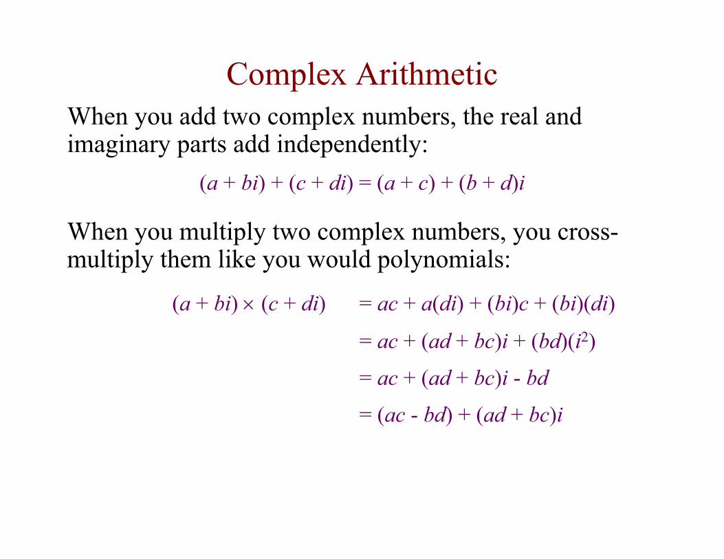
Complex ArithmeticWhen you add two complex numbers, the real and imaginary parts add independently:

(a + bi) + (c + di) = (a + c) + (b + d)i

When you multiply two complex numbers, you cross-multiply them like you would polynomials:

(a + bi) × (c + di) = ac + a(di) + (bi)c + (bi)(di)

= ac + (ad + bc)i + (bd)(i2)

= ac + (ad + bc)i - bd

= (ac - bd) + (ad + bc)i

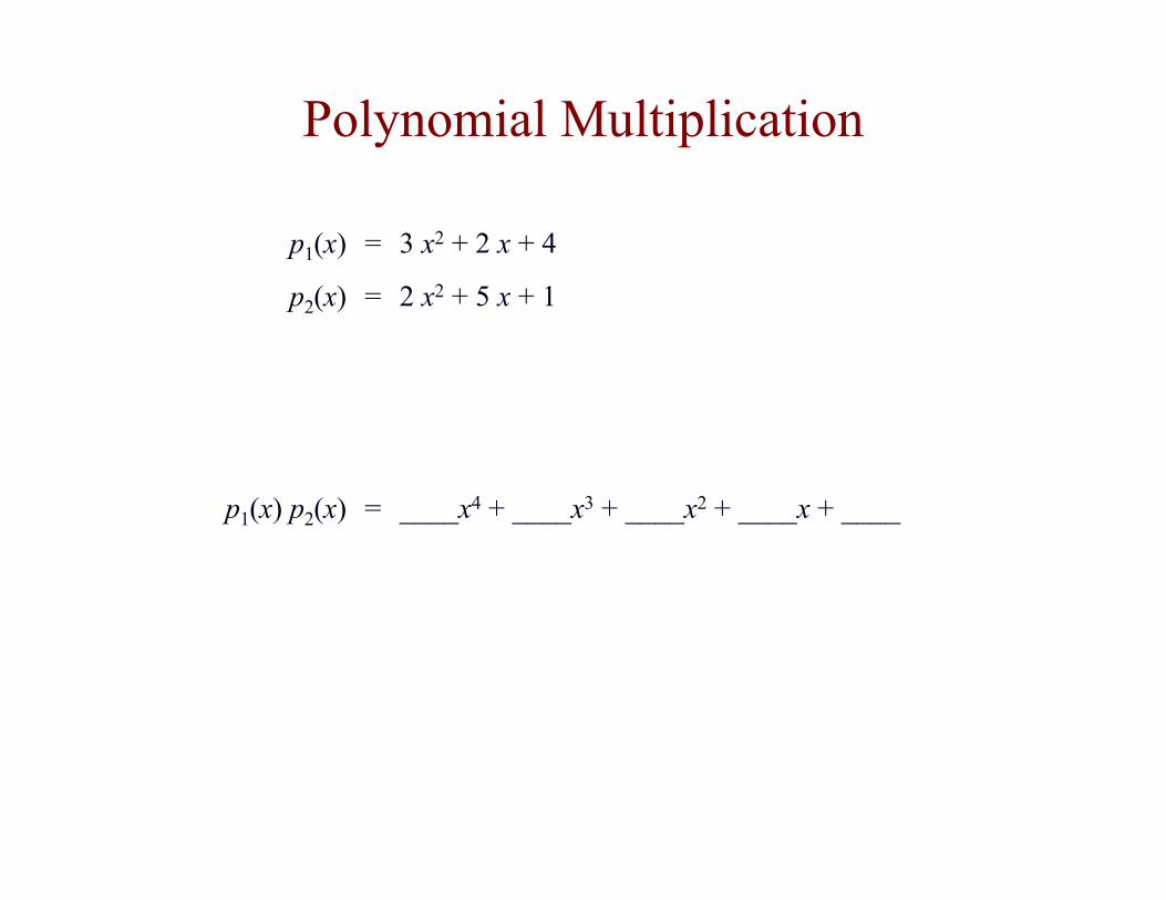
Polynomial Multiplication

p1(x) = 3 x2 + 2 x + 4

p2(x) = 2 x2 + 5 x + 1

p1(x) p2(x) = ____x4 + ____x3 + ____x2 + ____x + ____

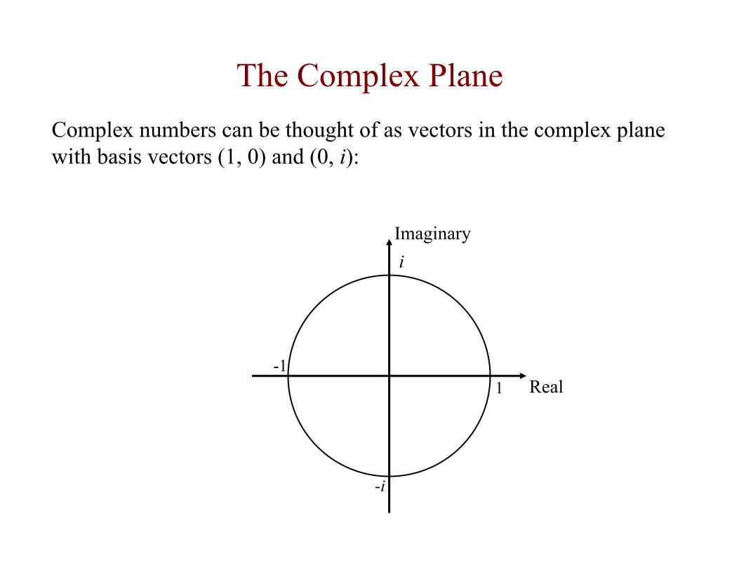
The Complex PlaneComplex numbers can be thought of as vectors in the complex plane with basis vectors (1, 0) and (0, i):

Real

Imaginary

1-1

i

-i

i

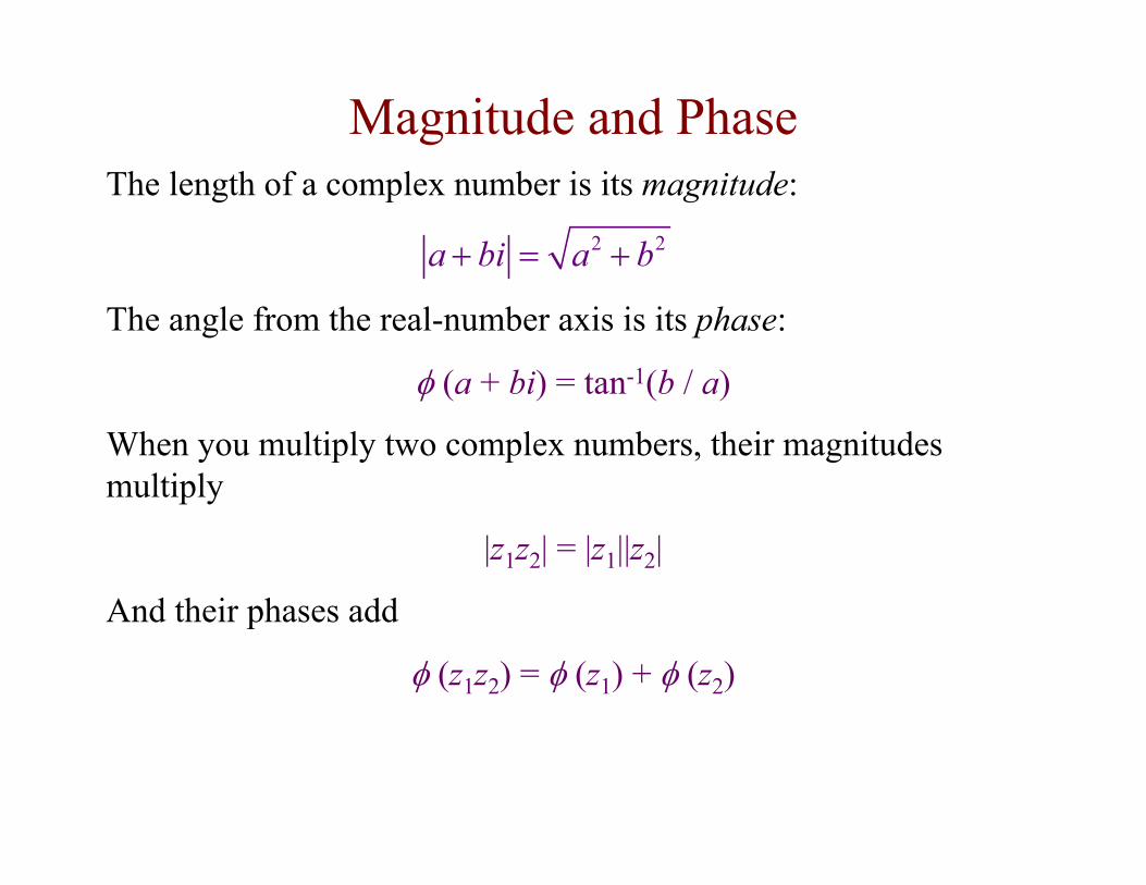
Magnitude and PhaseThe length of a complex number is its magnitude:

The angle from the real-number axis is its phase:

φ (a + bi) = tan-1(b / a)

When you multiply two complex numbers, their magnitudes multiply

|z1z2| = |z1||z2|

And their phases add

φ (z1z2) = φ (z1) + φ (z2)

2 2a bi a b+ = +

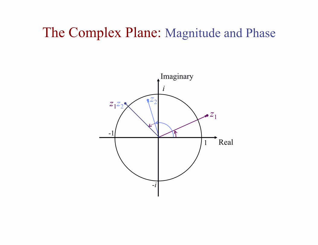
The Complex Plane: Magnitude and Phase

Real

Imaginary

1-1

i

-i

z1

z2z1z2

Real

Imaginary

1-1

i

-i

i

Complex ConjugatesIf z = a + bi is a complex number, then its complex conjugate is:

z* = a - bi

The complex conjugate z* has the same magnitude but opposite phase

When you add z to z*, the imaginary parts cancel and you get a real number:

(a + bi) + (a - bi) = 2a

When you multiply z to z*, you get the real number equal to |z|2:

(a + bi)(a - bi) = a2 – (bi)2 = a2 + b2

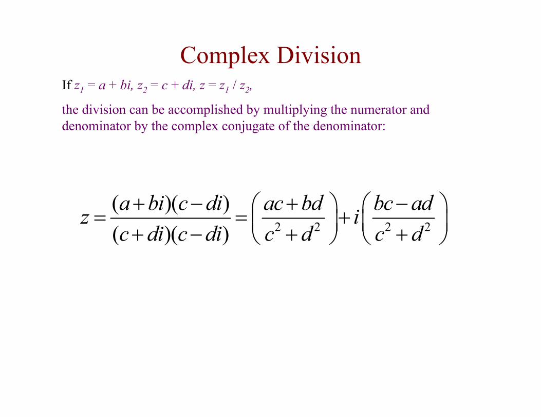
Complex DivisionIf z1 = a + bi, z2 = c + di, z = z1 / z2,

the division can be accomplished by multiplying the numerator and denominator by the complex conjugate of the denominator:

2 2 2 2

( )( )( )( )a bi c di ac bd bc adz ic di c di c d c d

+ − + −⎛ ⎞ ⎛ ⎞= = +⎜ ⎟ ⎜ ⎟+ − + +⎝ ⎠ ⎝ ⎠

Euler’s Formula

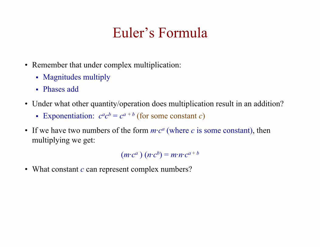
• Remember that under complex multiplication:Magnitudes multiplyPhases add

• Under what other quantity/operation does multiplication result in an addition?Exponentiation: cacb = ca + b (for some constant c)

• If we have two numbers of the form m·ca (where c is some constant), then multiplying we get:

(m·ca ) (n·cb) = m·n·ca + b

• What constant c can represent complex numbers?

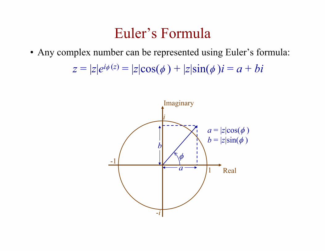
Euler’s Formula• Any complex number can be represented using Euler’s formula:

z = |z|eiφ (z) = |z|cos(φ ) + |z|sin(φ )i = a + bi

Real

Imaginary

1-1

i

-i

b

aφ

a = |z|cos(φ )b = |z|sin(φ )

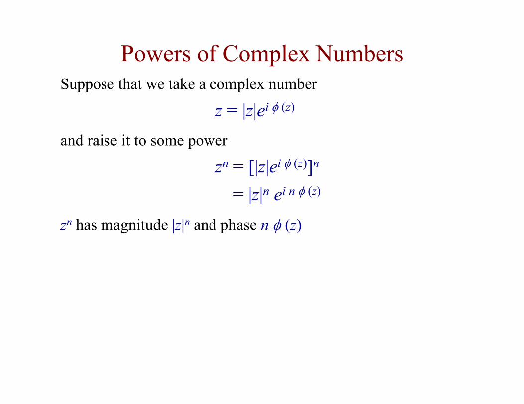
Powers of Complex NumbersSuppose that we take a complex number

z = |z|ei φ (z)

and raise it to some power

zn = [|z|ei φ (z)]n

= |z|n ei n φ (z)

zn has magnitude |z|n and phase n φ (z)

Real

Imaginary

1-1

i

-i

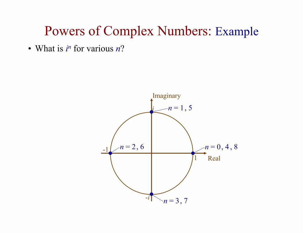
Powers of Complex Numbers: Example• What is in for various n?

, 4n = 0

, 5n = 1

n = 2, 6 , 8

n = 3, 7

Real

Imaginary

1-1

i

-i

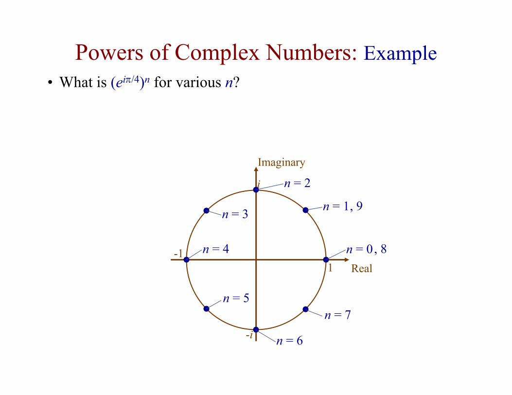
Powers of Complex Numbers: Example• What is (eiπ/4)n for various n?

, 8n = 0

, 9

n = 2

n = 4

n = 6

n = 1n = 3

n = 5n = 7

Real

Imaginary

1-1

i

-i

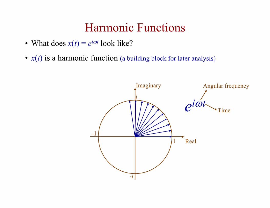
Harmonic Functions• What does x(t) = eiωt look like?

• x(t) is a harmonic function (a building block for later analysis)

eiωt

Angular frequency

Time

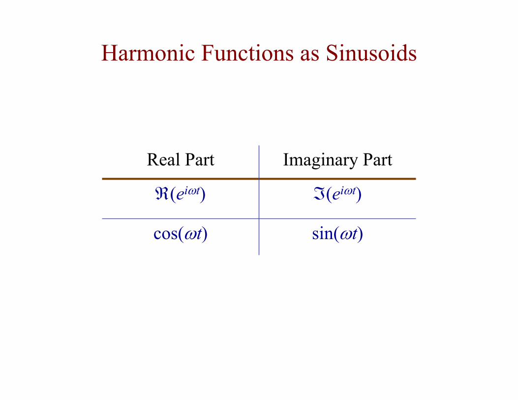
Harmonic Functions as Sinusoids

sin(ωt)cos(ωt)

ℑ(eiωt)ℜ(eiωt)

Imaginary PartReal Part

Questions: Complex Numbers

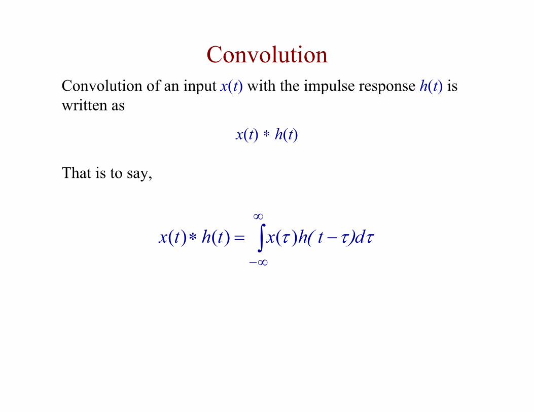
ConvolutionConvolution of an input x(t) with the impulse response h(t) is written as

x(t) * h(t)

That is to say,

ττ)(τ dthxthtx ∫∞

∞−

−=∗ )()()(

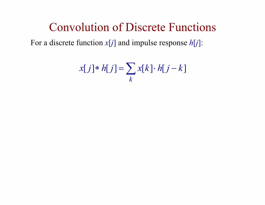
Convolution of Discrete FunctionsFor a discrete function x[j] and impulse response h[j]:

∑ −⋅=∗k

kjhkxjhjx ][][][][

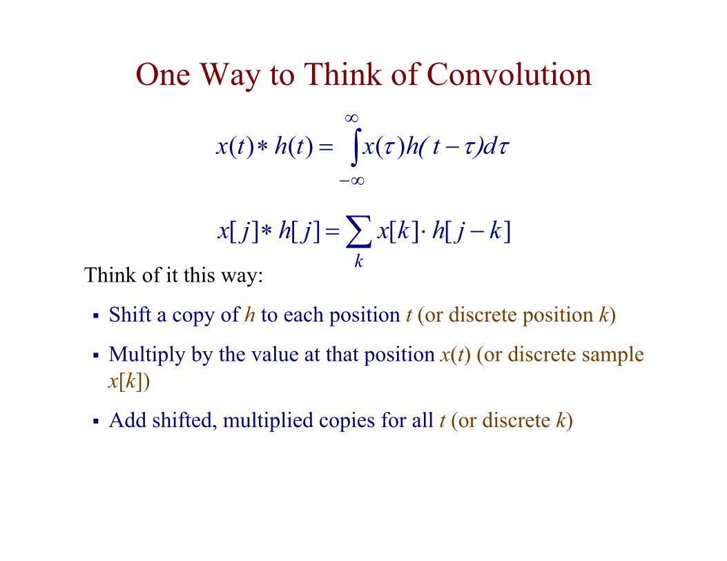
One Way to Think of Convolution

Think of it this way:

Shift a copy of h to each position t (or discrete position k)

Multiply by the value at that position x(t) (or discrete sample x[k])

Add shifted, multiplied copies for all t (or discrete k)

∑ −⋅=∗k

kjhkxjhjx ][][][][

ττ)(τ dthxthtx ∫∞

∞−

−=∗ )()()(

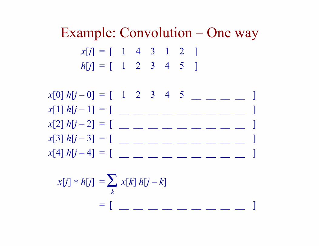
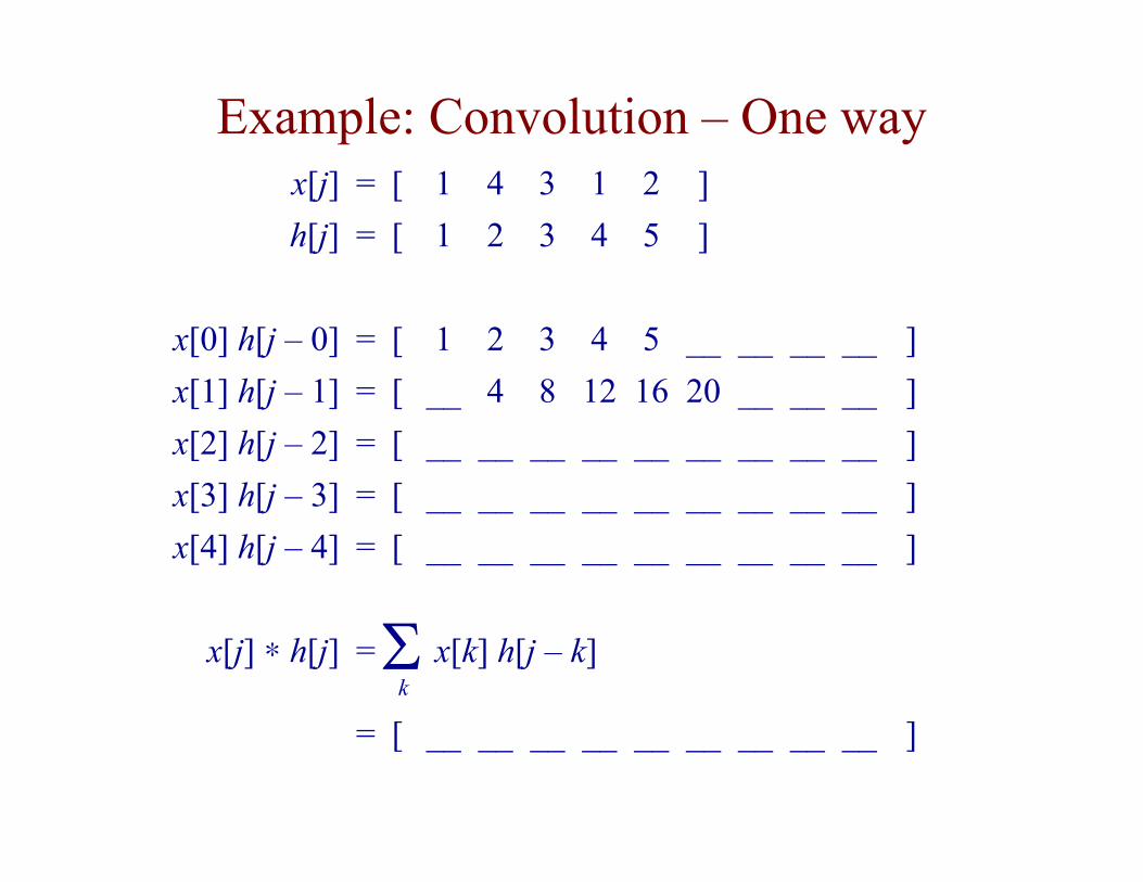
Example: Convolution – One wayx[j] = [ 1 4 3 1 2 ]h[j] = [ 1 2 3 4 5 ]

x[0] h[j – 0] = [ __ __ __ __ __ __ __ __ __ ]x[1] h[j – 1] = [ __ __ __ __ __ __ __ __ __ ]x[2] h[j – 2] = [ __ __ __ __ __ __ __ __ __ ]x[3] h[j – 3] = [ __ __ __ __ __ __ __ __ __ ]x[4] h[j – 4] = [ __ __ __ __ __ __ __ __ __ ]

x[j] * h[j] = x[k] h[j – k]

= [ __ __ __ __ __ __ __ __ __ ]

Σk

Example: Convolution – One wayx[j] = [ 1 4 3 1 2 ]h[j] = [ 1 2 3 4 5 ]

x[0] h[j – 0] = [ 1 2 3 4 5 __ __ __ __ ]x[1] h[j – 1] = [ __ __ __ __ __ __ __ __ __ ]x[2] h[j – 2] = [ __ __ __ __ __ __ __ __ __ ]x[3] h[j – 3] = [ __ __ __ __ __ __ __ __ __ ]x[4] h[j – 4] = [ __ __ __ __ __ __ __ __ __ ]

x[j] * h[j] = x[k] h[j – k]

= [ __ __ __ __ __ __ __ __ __ ]

Σk

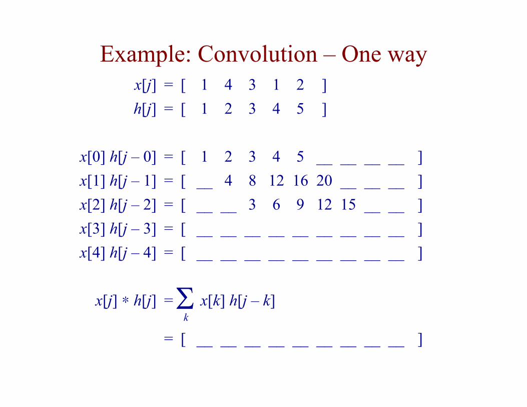
Example: Convolution – One wayx[j] = [ 1 4 3 1 2 ]h[j] = [ 1 2 3 4 5 ]

x[0] h[j – 0] = [ 1 2 3 4 5 __ __ __ __ ]x[1] h[j – 1] = [ __ 4 8 12 16 20 __ __ __ ] x[2] h[j – 2] = [ __ __ __ __ __ __ __ __ __ ]x[3] h[j – 3] = [ __ __ __ __ __ __ __ __ __ ]x[4] h[j – 4] = [ __ __ __ __ __ __ __ __ __ ]

x[j] * h[j] = x[k] h[j – k]

= [ __ __ __ __ __ __ __ __ __ ]

Σk

Example: Convolution – One wayx[j] = [ 1 4 3 1 2 ]h[j] = [ 1 2 3 4 5 ]

x[0] h[j – 0] = [ 1 2 3 4 5 __ __ __ __ ]x[1] h[j – 1] = [ __ 4 8 12 16 20 __ __ __ ] x[2] h[j – 2] = [ __ __ 3 6 9 12 15 __ __ ]x[3] h[j – 3] = [ __ __ __ __ __ __ __ __ __ ]x[4] h[j – 4] = [ __ __ __ __ __ __ __ __ __ ]

x[j] * h[j] = x[k] h[j – k]

= [ __ __ __ __ __ __ __ __ __ ]

Σk

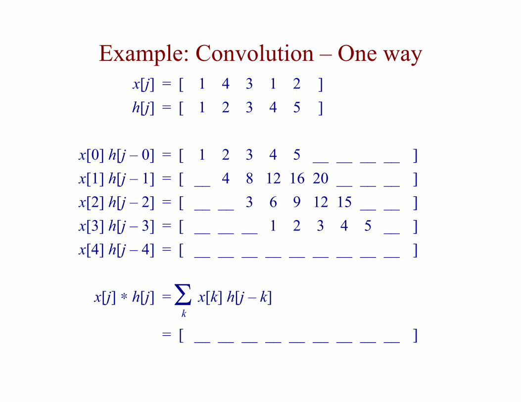
Example: Convolution – One wayx[j] = [ 1 4 3 1 2 ]h[j] = [ 1 2 3 4 5 ]

x[0] h[j – 0] = [ 1 2 3 4 5 __ __ __ __ ]x[1] h[j – 1] = [ __ 4 8 12 16 20 __ __ __ ] x[2] h[j – 2] = [ __ __ 3 6 9 12 15 __ __ ]x[3] h[j – 3] = [ __ __ __ 1 2 3 4 5 __ ]x[4] h[j – 4] = [ __ __ __ __ __ __ __ __ __ ]

x[j] * h[j] = x[k] h[j – k]

= [ __ __ __ __ __ __ __ __ __ ]

Σk

Example: Convolution – One wayx[j] = [ 1 4 3 1 2 ]h[j] = [ 1 2 3 4 5 ]

x[0] h[j – 0] = [ 1 2 3 4 5 __ __ __ __ ]x[1] h[j – 1] = [ __ 4 8 12 16 20 __ __ __ ] x[2] h[j – 2] = [ __ __ 3 6 9 12 15 __ __ ]x[3] h[j – 3] = [ __ __ __ 1 2 3 4 5 __ ]x[4] h[j – 4] = [ __ __ __ __ 2 4 6 8 10 ]

x[j] * h[j] = x[k] h[j – k]

= [ __ __ __ __ __ __ __ __ __ ]

Σk

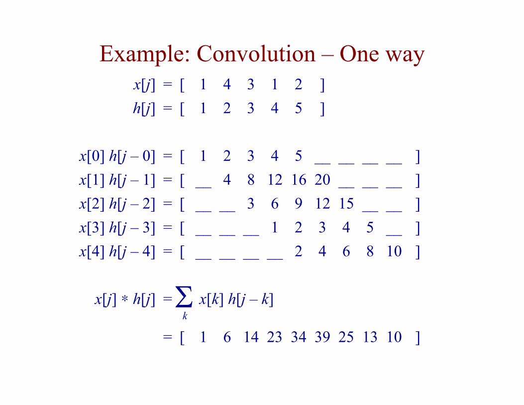
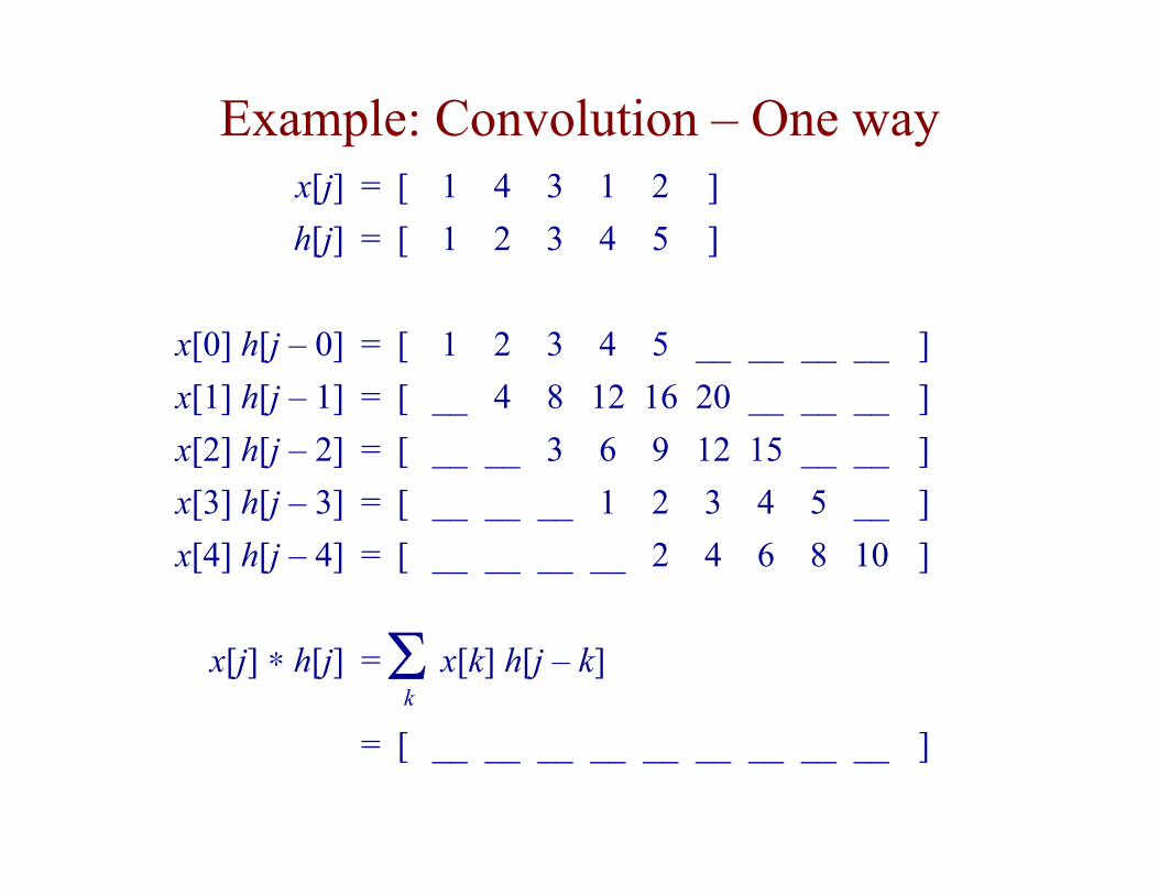
Example: Convolution – One wayx[j] = [ 1 4 3 1 2 ]h[j] = [ 1 2 3 4 5 ]

x[0] h[j – 0] = [ 1 2 3 4 5 __ __ __ __ ]x[1] h[j – 1] = [ __ 4 8 12 16 20 __ __ __ ] x[2] h[j – 2] = [ __ __ 3 6 9 12 15 __ __ ]x[3] h[j – 3] = [ __ __ __ 1 2 3 4 5 __ ]x[4] h[j – 4] = [ __ __ __ __ 2 4 6 8 10 ]

x[j] * h[j] = x[k] h[j – k]

= [ 1 6 14 23 34 39 25 13 10 ]

Σk

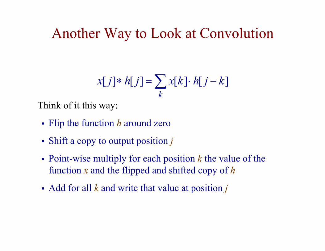
Another Way to Look at Convolution

Think of it this way:

Flip the function h around zero

Shift a copy to output position j

Point-wise multiply for each position k the value of the function x and the flipped and shifted copy of h

Add for all k and write that value at position j

∑ −⋅=∗k

kjhkxjhjx ][][][][

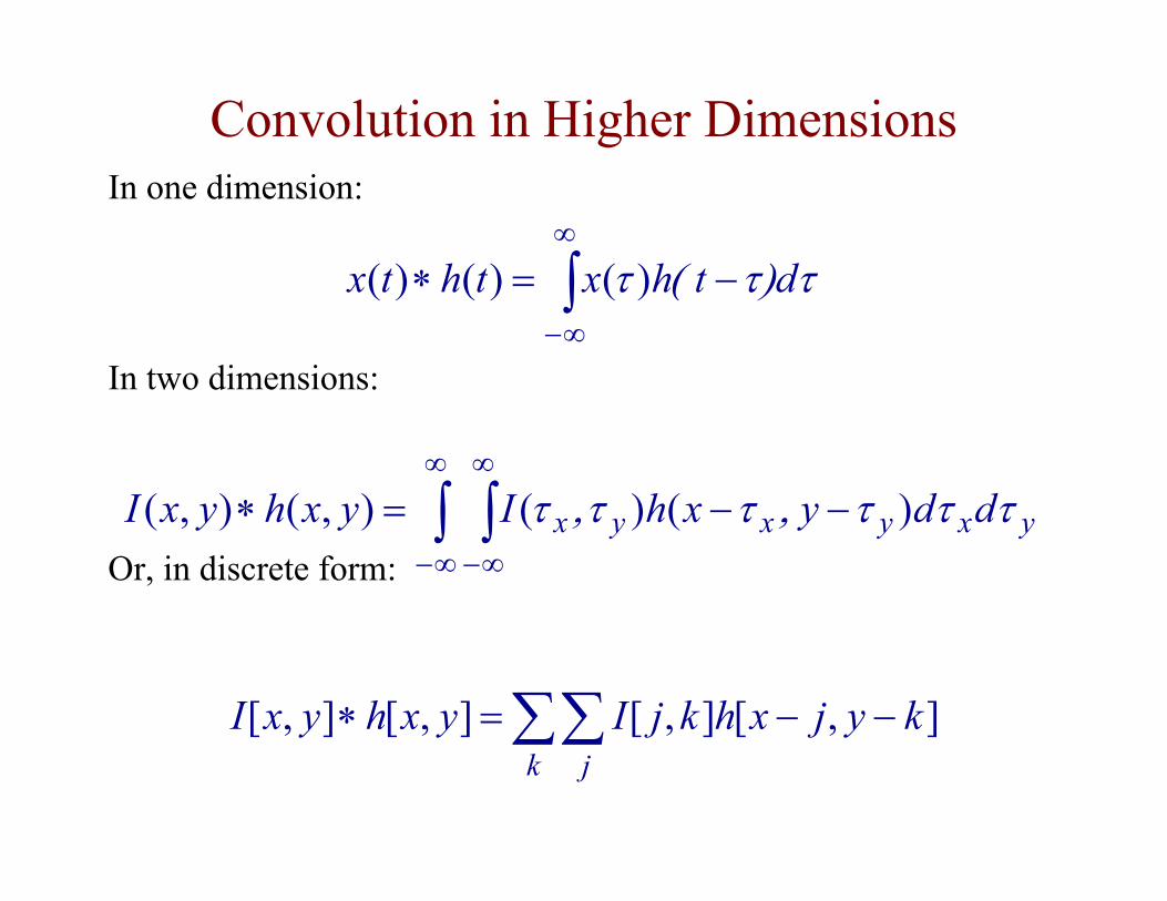
Convolution in Higher DimensionsIn one dimension:

In two dimensions:

Or, in discrete form:

ττ)(τ dthxthtx ∫∞

∞−

−=∗ )()()(

∫ ∫∞

∞−

∞

∞−

−−=∗ yxyxyx ddyxhIyxhyxI τττ,ττ,τ )()(),(),(

∑∑ −−=∗k j

kyjxhkjIyxhyxI ],[],[],[],[

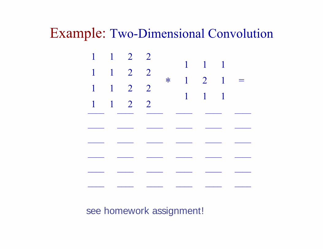
Example: Two-Dimensional Convolution

____ ____ ____ ____ ____ ____

____ ____ ____ ____ ____ ____

____ ____ ____ ____ ____ ____

____ ____ ____ ____ ____ ____

____ ____ ____ ____ ____ ____

____ ____ ____ ____ ____ ____

1 1 2 21 1 2 21 1 2 21 1 2 2

1 1 1* 1 2 1 =

1 1 1

see homework assignment!

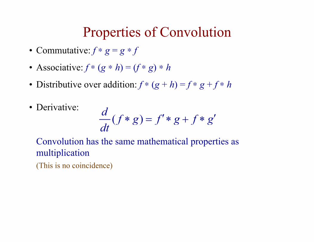
Properties of Convolution• Commutative: f * g = g * f

• Associative: f * (g * h) = (f * g) * h

• Distributive over addition: f * (g + h) = f * g + f * h

• Derivative:

Convolution has the same mathematical properties as multiplication(This is no coincidence)

( )d f g f g f gdt

′ ′∗ = ∗ + ∗

Useful Functions• Square: Πa(t)

• Triangle: Λa(t)

• Gaussian: G(t, s)

• Step: u(t)

• Impulse/Delta: δ (t)

• Comb (Shah Function): combh(t)

Each has their two- or three-dimensional equivalent.

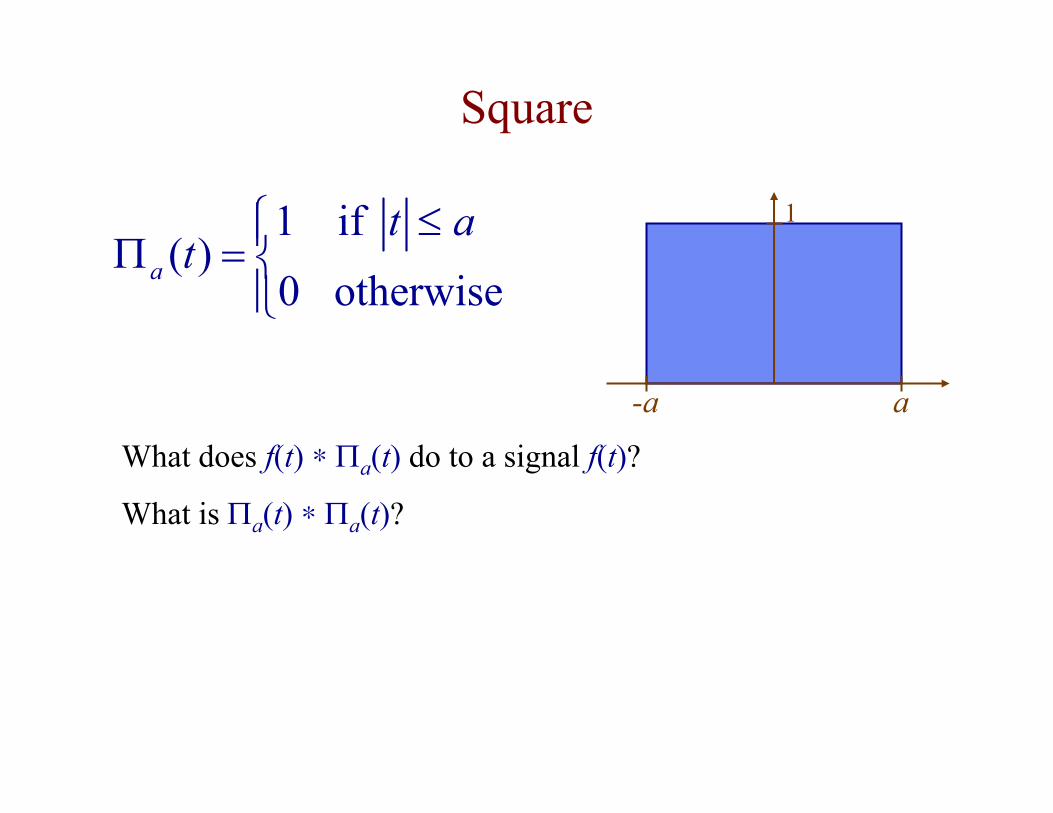
Square

What does f(t) * Πa(t) do to a signal f(t)?

What is Πa(t) * Πa(t)?

-a a

11 if ( )

0 otherwisea

t at

⎧ ≤⎪Π = ⎨⎪⎩

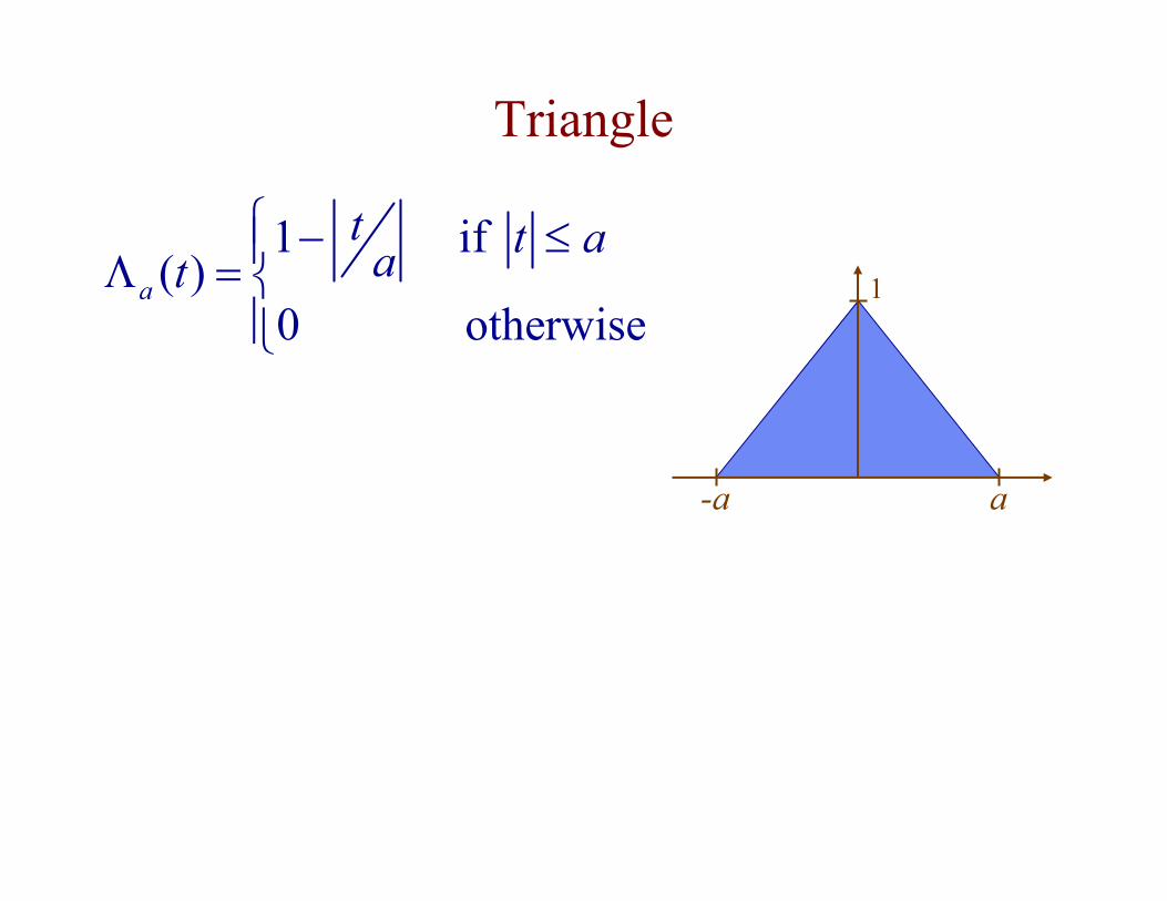
Triangle

-a a

11 if

( )0 otherwise

a

t t aat⎧ − ≤⎪Λ = ⎨⎪⎩

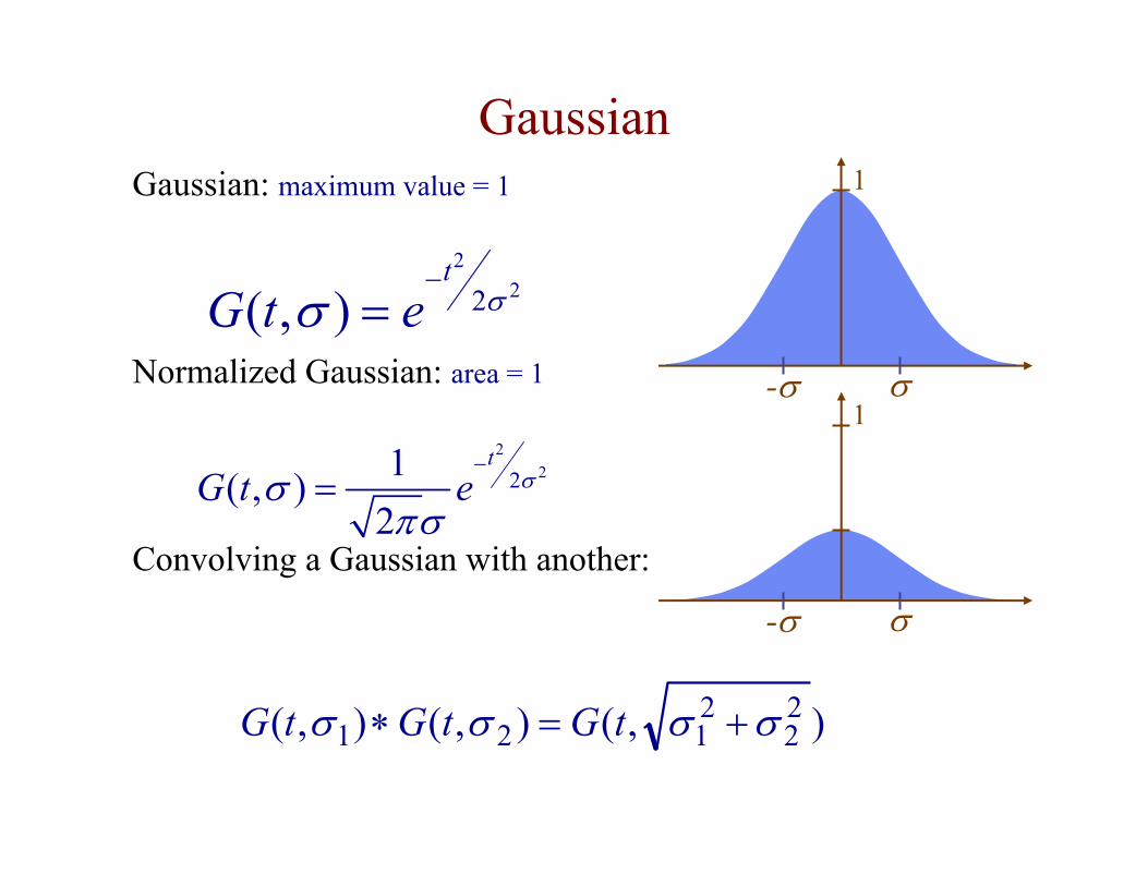
GaussianGaussian: maximum value = 1

Normalized Gaussian: area = 1

Convolving a Gaussian with another:

-σ σ

1

-σ σ

1

222( , )

tG t e σσ

−=

2221( , )

2

tG t e σσ

πσ−

=

),(),(),( 22

2121 σσσσ +=∗ tGtGtG

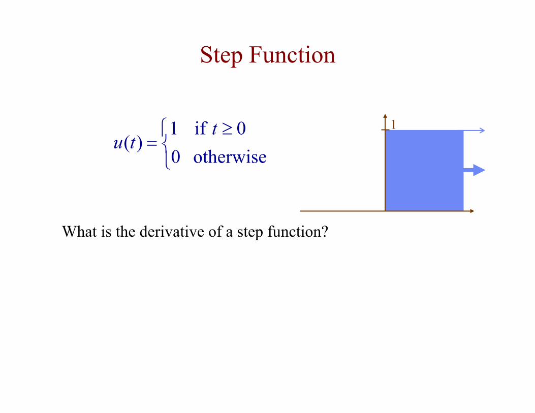
Step Function

What is the derivative of a step function?

1

⎩⎨⎧ ≥

=otherwise 0

0 if 1)(

ttu

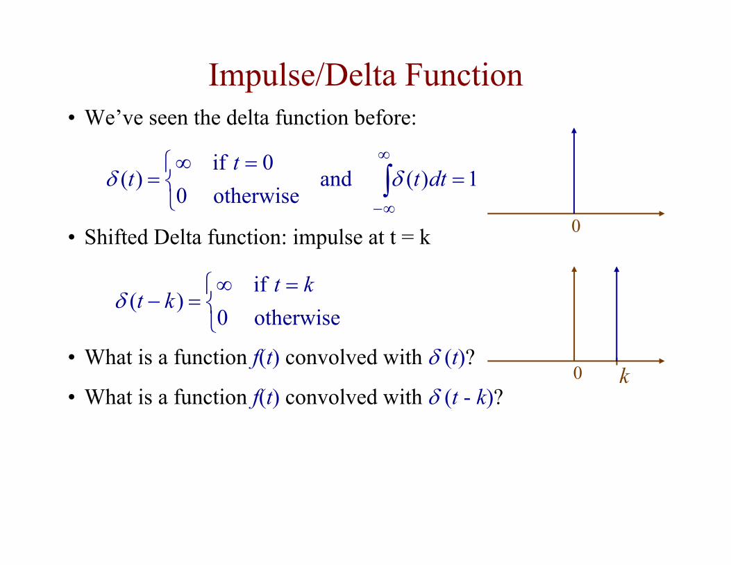
Impulse/Delta Function• We’ve seen the delta function before:

• Shifted Delta function: impulse at t = k

• What is a function f(t) convolved with δ (t)?

• What is a function f(t) convolved with δ (t - k)?

0

k0

∫∞

∞−

=⎩⎨⎧ =∞

= 1)( and otherwise 0

0 if )( dtt

tt δδ

⎩⎨⎧ =∞

=−otherwise 0

if )(

ktktδ

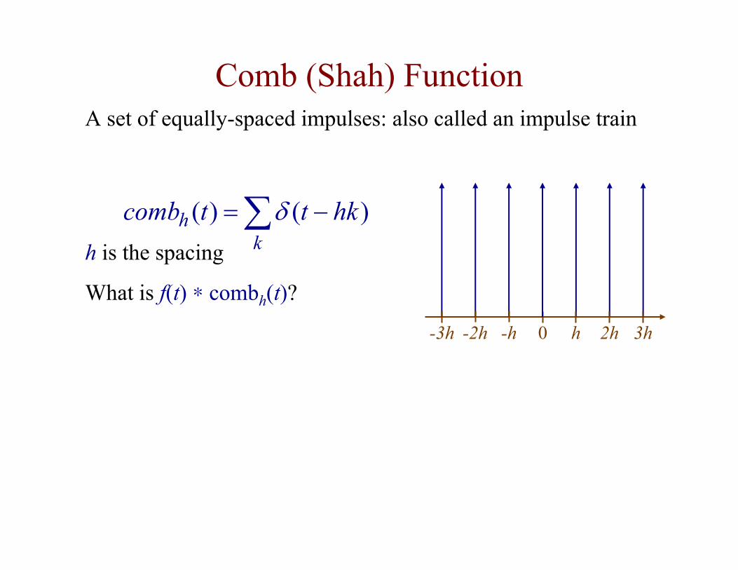
Comb (Shah) FunctionA set of equally-spaced impulses: also called an impulse train

h is the spacing

What is f(t) * combh(t)?

-2h h-h 2h 3h0-3h

∑ −=k

h hkttcomb )()( δ

Convolution Filtering• Convolution is useful for modeling the behavior of filters

• It is also useful to do ourselves to produce a desired effect

• When we do it ourselves, we get to choose the function that the input will be convolved with

• This function that is convolved with the input is called the convolution kernel

Convolution Filtering: AveragingCan use a square function (“box filter”) or Gaussian to locally average the signal/image

Square (box) function: uniform averagingGaussian: center-weighted averaging

Both of these blur the signal or image

Questions: Convolution

Frequency Analysis

© http://www.cs.sfu.ca/~hamarneh/courses/cmpt340_04_1© http://www.physics.gatech.edu/gcuo/UltrafastOptics/PhysicalOptics/

Here, we write a square wave as a sum of sine waves:

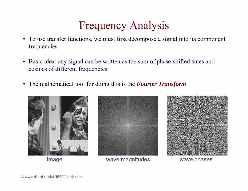
Frequency Analysis• To use transfer functions, we must first decompose a signal into its component

frequencies

• Basic idea: any signal can be written as the sum of phase-shifted sines and cosines of different frequencies

• The mathematical tool for doing this is the Fourier Transform

© www.dai.ed.ac.uk/HIPR2/ fourier.htm

image wave magnitudes wave phases

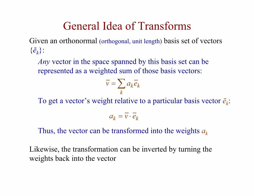
General Idea of TransformsGiven an orthonormal (orthogonal, unit length) basis set of vectors {ēk}:

Any vector in the space spanned by this basis set can be represented as a weighted sum of those basis vectors:

To get a vector’s weight relative to a particular basis vector ēk:

Thus, the vector can be transformed into the weights ak

Likewise, the transformation can be inverted by turning the weights back into the vector

∑=k

kkeav

kk eva ⋅=

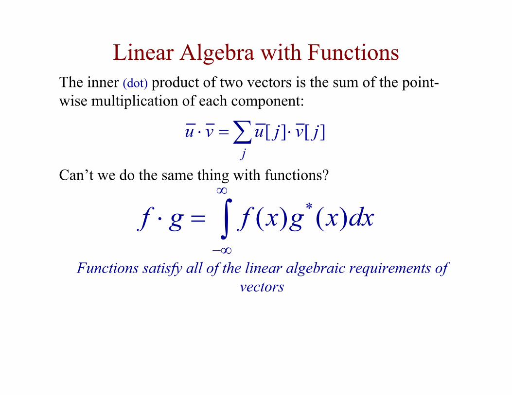
Linear Algebra with FunctionsThe inner (dot) product of two vectors is the sum of the point-wise multiplication of each component:

Can’t we do the same thing with functions?

Functions satisfy all of the linear algebraic requirements of vectors

∑ ⋅=⋅j

jvjuvu ][][

*( ) ( )f g f x g x dx∞

−∞

⋅ = ∫

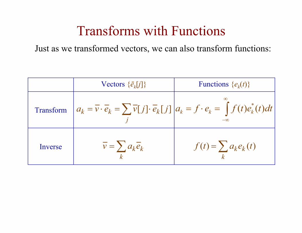
Transforms with FunctionsJust as we transformed vectors, we can also transform functions:

Inverse

Transform

Functions {ek(t)}Vectors {ēk[j]}

∑ ⋅=⋅=j

kkk jejveva ][][

∑=k

kkeav

*( ) ( )k k ka f e f t e t dt∞

−∞

= ⋅ = ∫

)()( teatfk

kk∑=

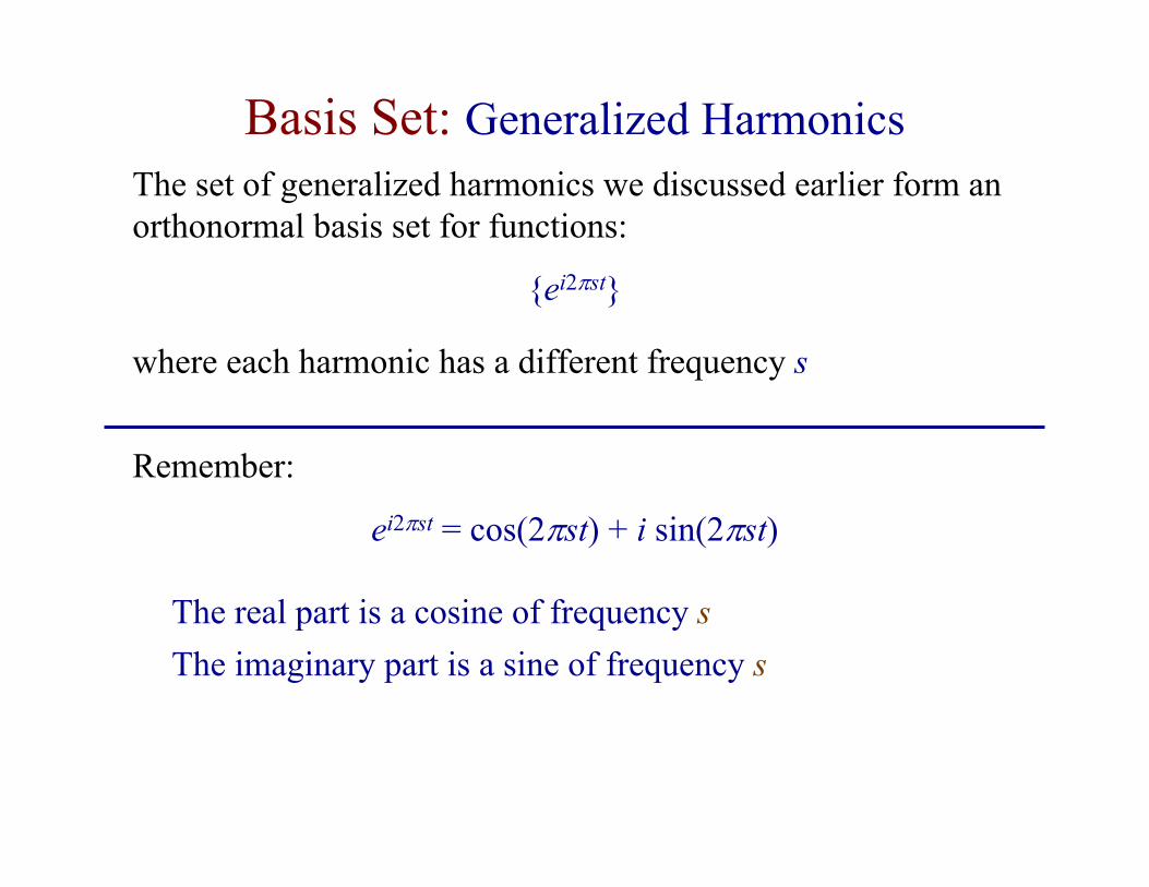
Basis Set: Generalized HarmonicsThe set of generalized harmonics we discussed earlier form an orthonormal basis set for functions:

{ei2πst}

where each harmonic has a different frequency s

Remember:

ei2πst = cos(2πst) + i sin(2πst)

The real part is a cosine of frequency sThe imaginary part is a sine of frequency s

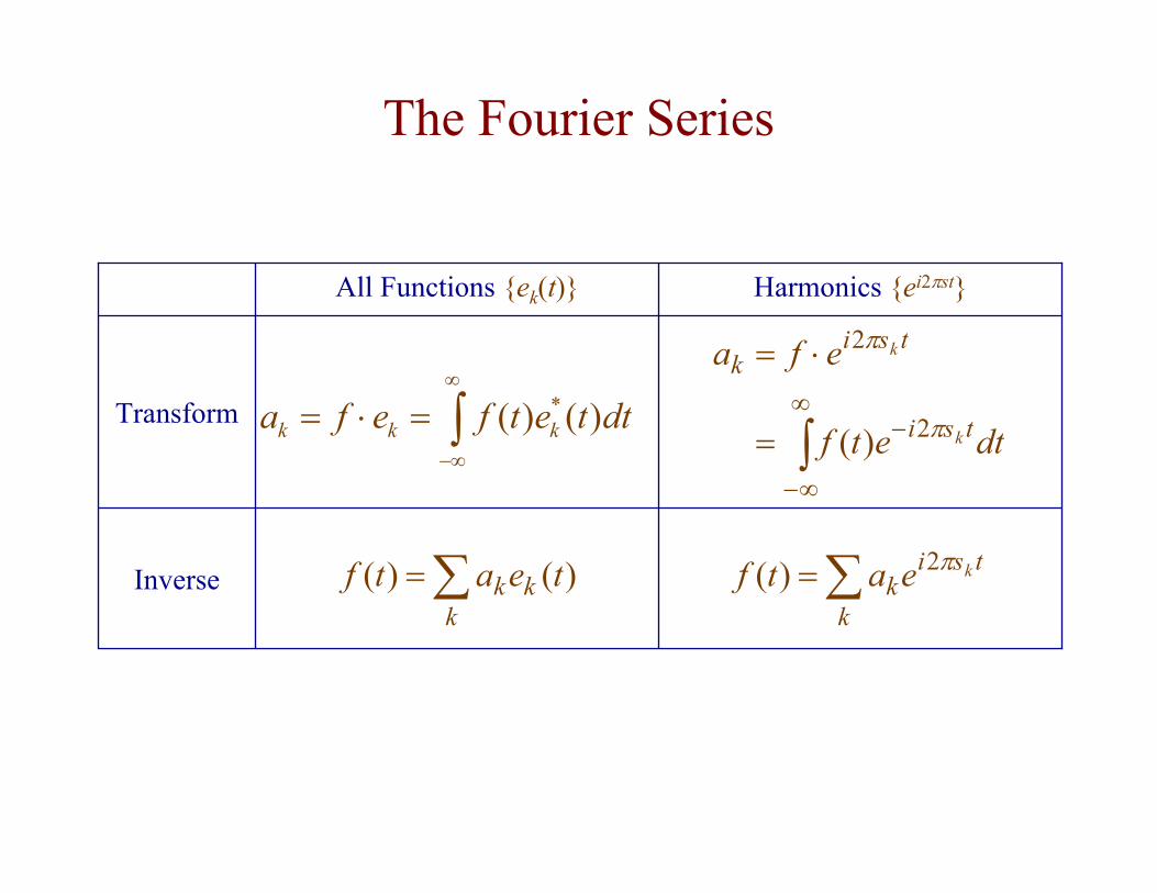
The Fourier Series

Inverse

Transform

Harmonics {ei2πst}All Functions {ek(t)}

*( ) ( )k k ka f e f t e t dt∞

−∞

= ⋅ = ∫

)()( teatfk

kk∑=

∫∞

∞−

−=

⋅=

dtetf

efa

tsi

tsik

k

k

π

π

2

2

)(

∑=k

tsik

keatf π2)(

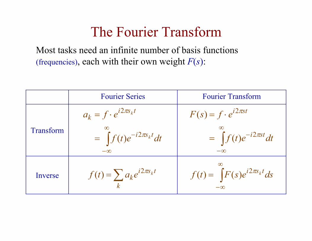
The Fourier TransformMost tasks need an infinite number of basis functions (frequencies), each with their own weight F(s):

Inverse

Transform

Fourier TransformFourier Series

∫∞

∞−

−=

⋅=

dtetf

efsF

sti

sti

π

π

2

2

)(

)(

∫∞

∞−

= dsesFtf tsi kπ2)()(

∫∞

∞−

−=

⋅=

dtetf

efa

tsi

tsik

k

k

π

π

2

2

)(

∑=k

tsik

keatf π2)(

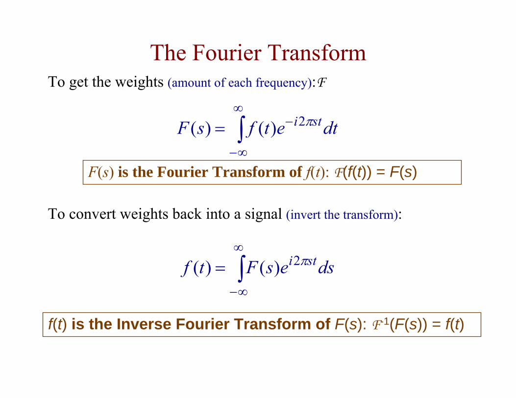
The Fourier TransformTo get the weights (amount of each frequency):F

To convert weights back into a signal (invert the transform):

F(s) is the Fourier Transform of f(t): F(f(t)) = F(s)

f(t) is the Inverse Fourier Transform of F(s): F-1(F(s)) = f(t)

∫∞

∞−

−= dtetfsF sti π2)()(

∫∞

∞−

= dsesFtf sti π2)()(

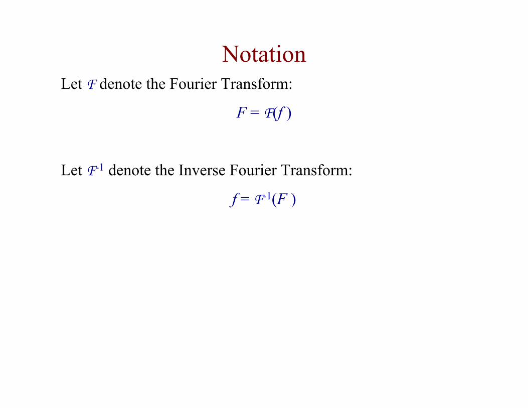
NotationLet F denote the Fourier Transform:

F = F(f )

Let F-1 denote the Inverse Fourier Transform:

f = F-1(F )

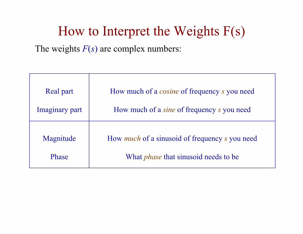
How to Interpret the Weights F(s)The weights F(s) are complex numbers:

How much of a sinusoid of frequency s you need

What phase that sinusoid needs to be

Magnitude

Phase

How much of a cosine of frequency s you need

How much of a sine of frequency s you need

Real part

Imaginary part

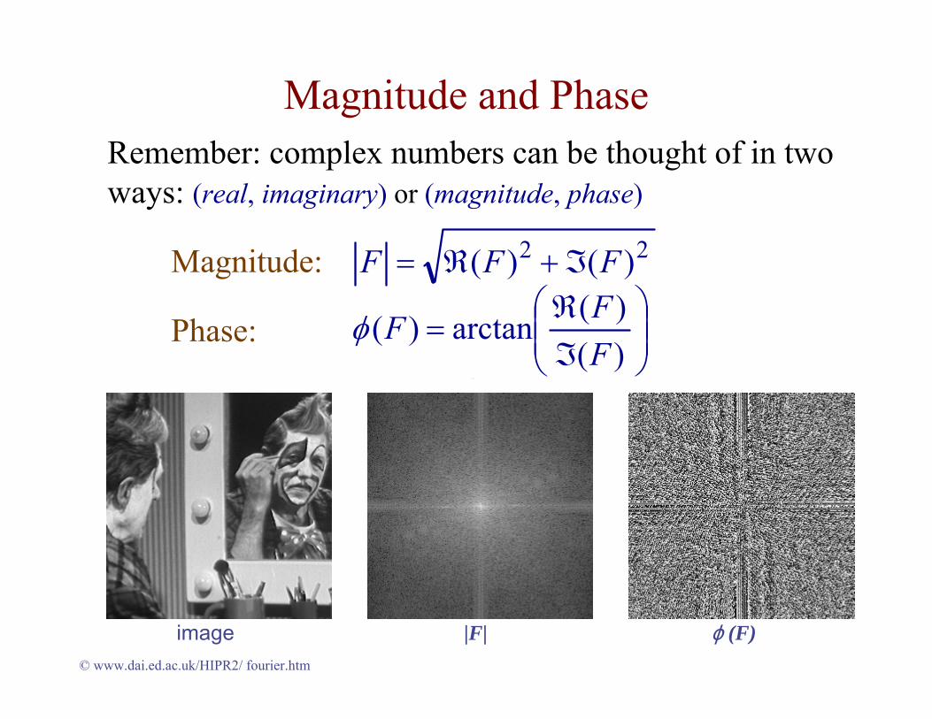
Magnitude and PhaseRemember: complex numbers can be thought of in two ways: (real, imaginary) or (magnitude, phase)

Magnitude:

Phase:

22 )()( FFF ℑ+ℜ=

⎟⎟⎠

⎞⎜⎜⎝

⎛ℑℜ

=)()(arctan)(

FFFφ

© www.dai.ed.ac.uk/HIPR2/ fourier.htm

image |F| ɸ (F)

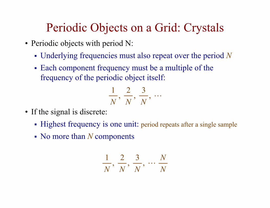
Periodic Objects on a Grid: Crystals• Periodic objects with period N:

Underlying frequencies must also repeat over the period NEach component frequency must be a multiple of the frequency of the periodic object itself:

• If the signal is discrete:Highest frequency is one unit: period repeats after a single sample

No more than N components

,3 ,2 ,1NNN

NN

NNN ,3 ,2 ,1

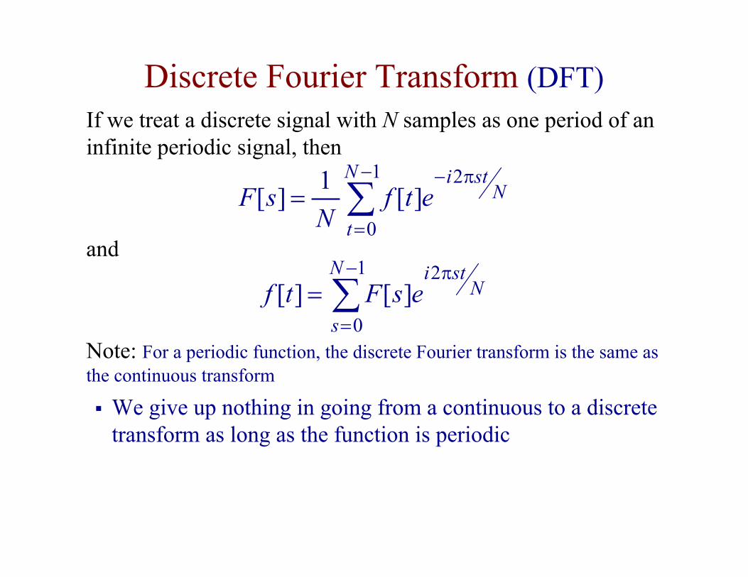
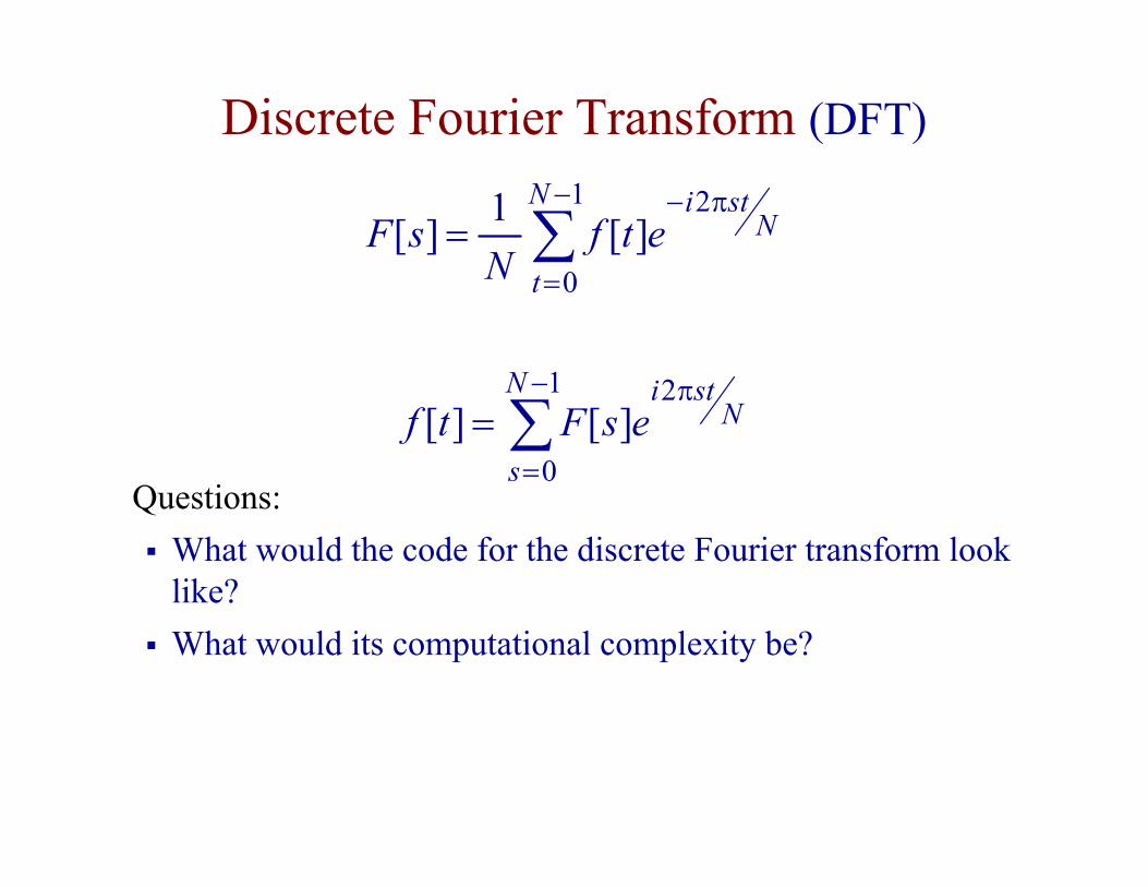
Discrete Fourier Transform (DFT)If we treat a discrete signal with N samples as one period of an infinite periodic signal, then

and

Note: For a periodic function, the discrete Fourier transform is the same as the continuous transform

We give up nothing in going from a continuous to a discrete transform as long as the function is periodic

∑−

=

π−=

1

0

2][1][

N

t

Nsti

etfN

sF

∑−

=

π=

1

0

2][][

N

s

Nsti

esFtf

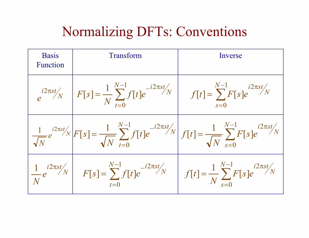
Normalizing DFTs: ConventionsInverseTransformBasis

Function

∑−

=

π−=

1

0

2][1][

N

t

Nsti

etfN

sF

Nsti

eN

π21

Nsti

eN

π21

∑−

=

π−=

1

0

2][1][

N

t

Nsti

etfN

sF

∑−

=

π−=

1

0

2][][

N

t

Nsti

etfsF

∑−

=

π=

1

0

2][][

N

s

Nsti

esFtf

∑−

=

π=

1

0

2][1][

N

s

Nsti

esFN

tf

∑−

=

π=

1

0

2][1][

N

s

Nsti

esFN

tf

Nsti

eπ2

Discrete Fourier Transform (DFT)

Questions:What would the code for the discrete Fourier transform look like?What would its computational complexity be?

∑−

=

π−=

1

0

2][1][

N

t

Nsti

etfN

sF

∑−

=

π=

1

0

2][][

N

s

Nsti

esFtf

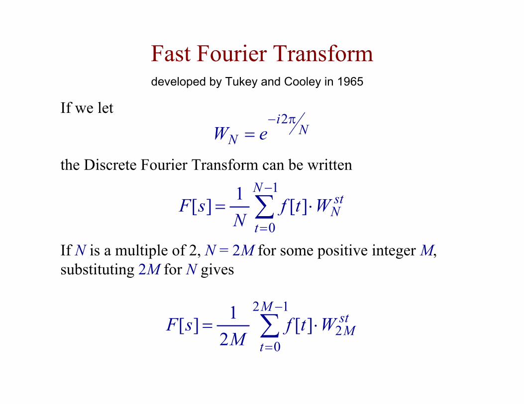
Fast Fourier Transform

If we let

the Discrete Fourier Transform can be written

If N is a multiple of 2, N = 2M for some positive integer M, substituting 2M for N gives

Ni

N eWπ−

=2

∑−

=⋅=

1

0][1][

N

t

stNWtf

NsF

∑−

=⋅=

12

02][

21][

M

t

stMWtf

MsF

developed by Tukey and Cooley in 1965

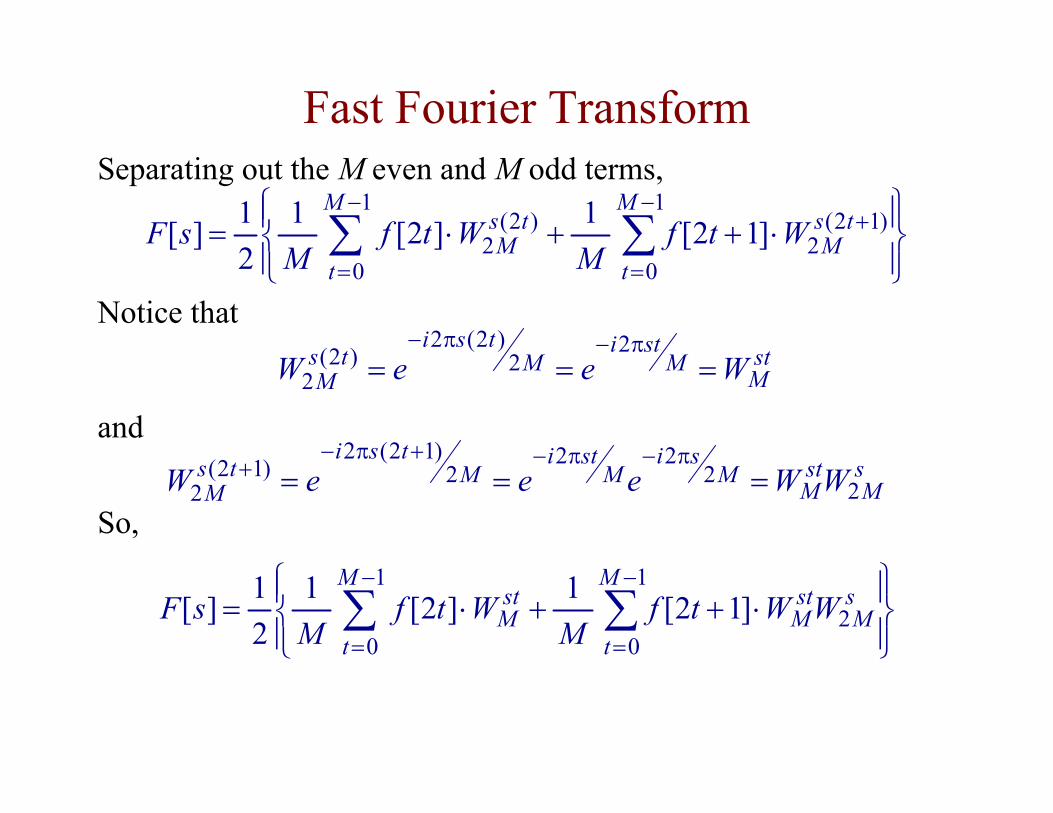
Fast Fourier TransformSeparating out the M even and M odd terms,

Notice that

and

So,

⎪⎭

⎪⎬⎫

⎪⎩

⎪⎨⎧

⋅++⋅= ∑ ∑−

=

−

=

+1

0

1

0

)12(2

)2(2 ]12[1]2[1

21][

M

t

M

t

tsM

tsM Wtf

MWtf

MsF

stM

Msti

Mtsi

tsM WeeW ===

π−π− 22

)2(2)2(

2

sM

stM

Msi

Msti

Mtsi

tsM WWeeeW 2

222

2)12(2

)12(2 ===

π−π−+π−+

⎪⎭

⎪⎬⎫

⎪⎩

⎪⎨⎧

⋅++⋅= ∑ ∑−

=

−

=

1

0

1

02]12[1]2[1

21][

M

t

M

t

sM

stM

stM WWtf

MWtf

MsF

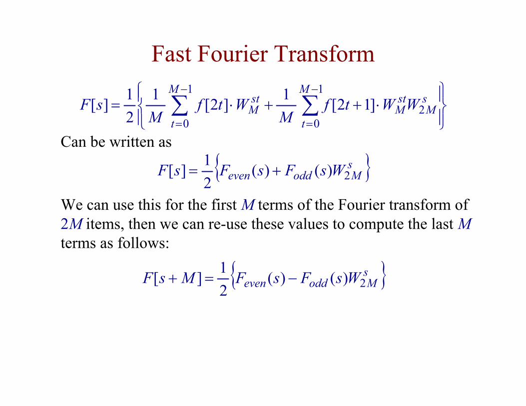
Fast Fourier Transform

Can be written as

We can use this for the first M terms of the Fourier transform of 2M items, then we can re-use these values to compute the last Mterms as follows:

⎪⎭

⎪⎬⎫

⎪⎩

⎪⎨⎧

⋅++⋅= ∑ ∑−

=

−

=

1

0

1

02]12[1]2[1

21][

M

t

M

t

sM

stM

stM WWtf

MWtf

MsF

{ }sModdeven WsFsFsF 2)()(

21][ +=

{ }sModdeven WsFsFMsF 2)()(

21][ −=+

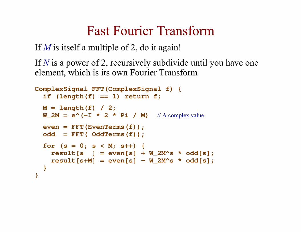
Fast Fourier TransformIf M is itself a multiple of 2, do it again!

If N is a power of 2, recursively subdivide until you have one element, which is its own Fourier Transform

ComplexSignal FFT(ComplexSignal f) {if (length(f) == 1) return f;

M = length(f) / 2;W_2M = e^(-I * 2 * Pi / M) // A complex value.

even = FFT(EvenTerms(f));odd = FFT( OddTerms(f));

for (s = 0; s < M; s++) {result[s ] = even[s] + W_2M^s * odd[s];result[s+M] = even[s] – W_2M^s * odd[s];

}}

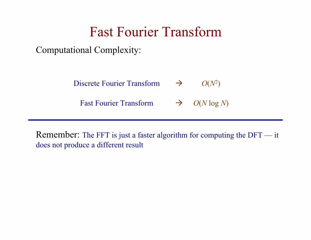
Fast Fourier TransformComputational Complexity:

Remember: The FFT is just a faster algorithm for computing the DFT — it does not produce a different result

O(N log N)Fast Fourier Transform

O(N2)Discrete Fourier Transform

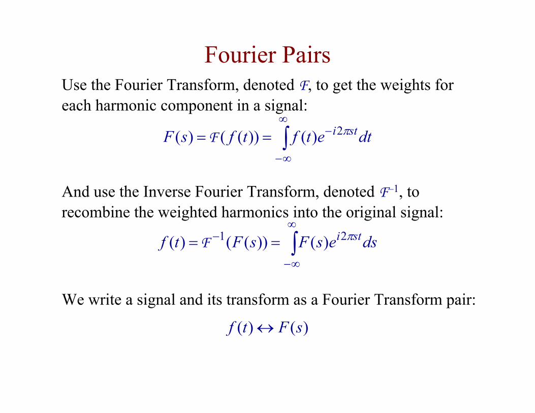
Fourier PairsUse the Fourier Transform, denoted F, to get the weights for each harmonic component in a signal:

And use the Inverse Fourier Transform, denoted F–1, to recombine the weighted harmonics into the original signal:

We write a signal and its transform as a Fourier Transform pair:

∫∞

∞−

−== dtetftfsF sti π2)())(()( F

∫∞

∞−

− == dsesFsFtf sti π21 )())(()( F

)()( sFtf ↔

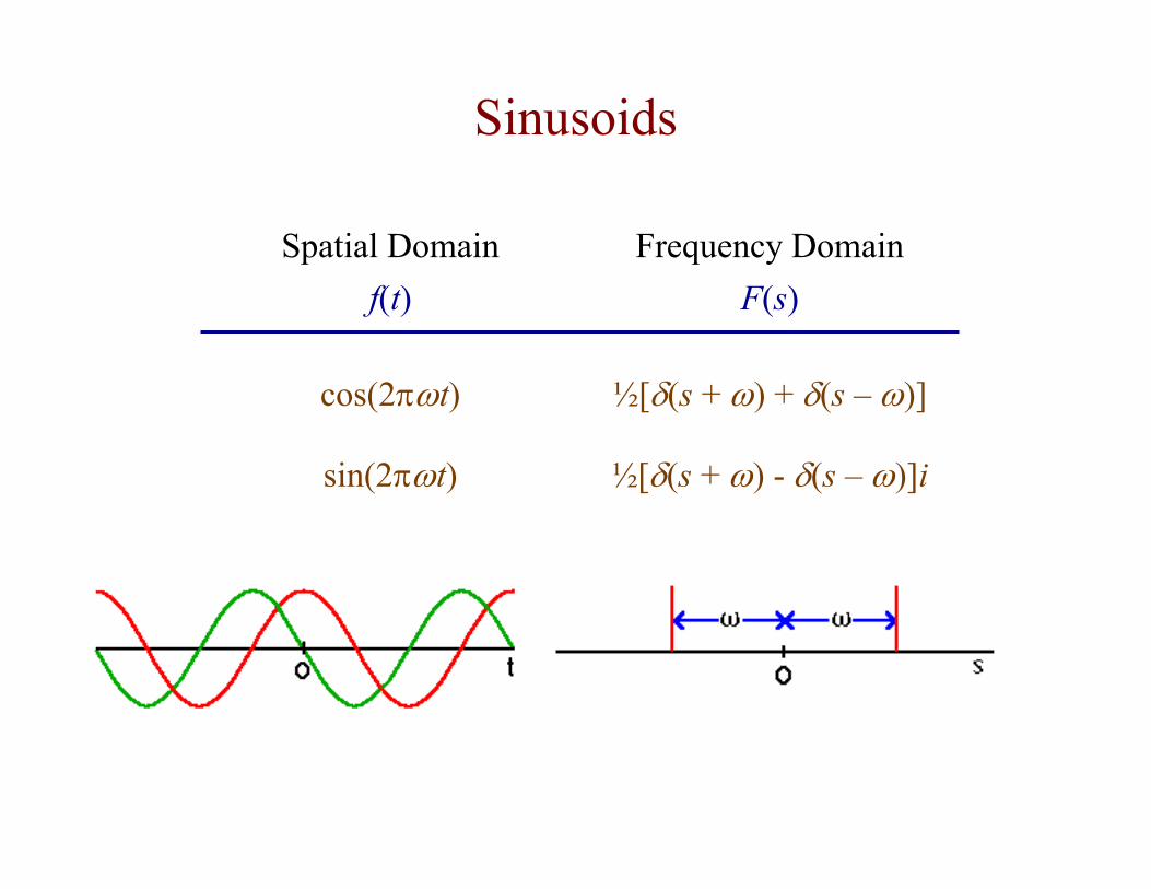
Sinusoids

½[δ(s + ω) + δ(s – ω)]

½[δ(s + ω) - δ(s – ω)]i

cos(2πωt)

sin(2πωt)

Frequency DomainF(s)

Spatial Domainf(t)

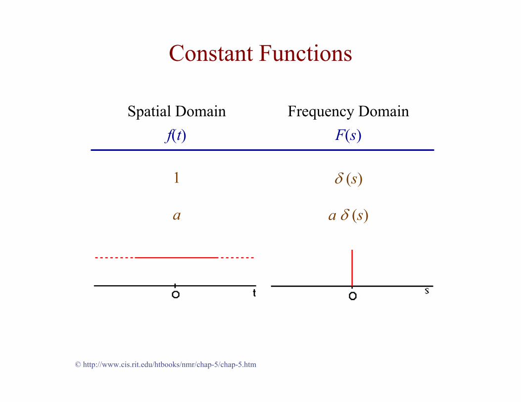
Constant Functions

δ (s)

a δ (s)

1

a

Frequency DomainF(s)

Spatial Domainf(t)

© http://www.cis.rit.edu/htbooks/nmr/chap-5/chap-5.htm

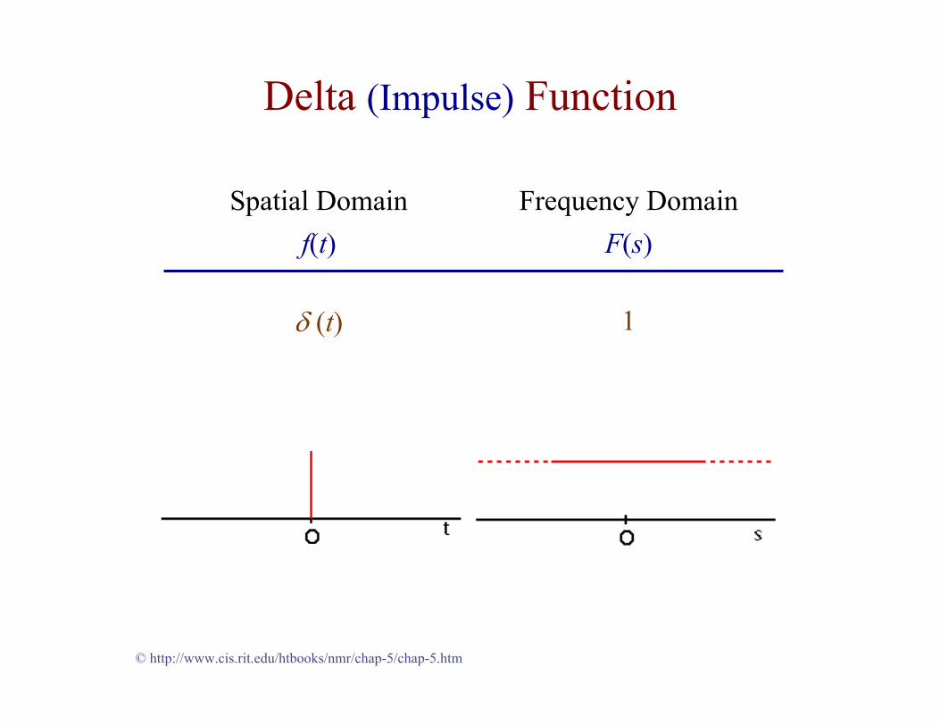
Delta (Impulse) Function

1δ (t)

Frequency DomainF(s)

Spatial Domainf(t)

© http://www.cis.rit.edu/htbooks/nmr/chap-5/chap-5.htm

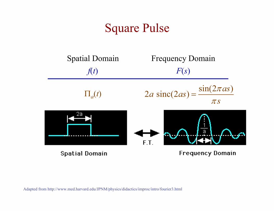
Square Pulse

Πa(t)

Frequency DomainF(s)

Spatial Domainf(t)

sin(2 )2 sinc(2 ) asa assπ

π=

Adapted from http://www.med.harvard.edu/JPNM/physics/didactics/improc/intro/fourier3.html

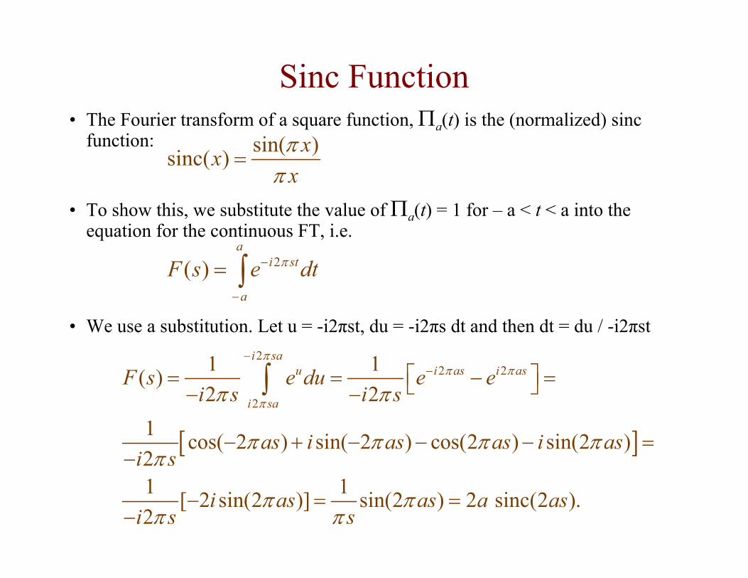
Sinc Function • The Fourier transform of a square function, Πa(t) is the (normalized) sinc

function:

• To show this, we substitute the value of Πa(t) = 1 for – a < t < a into the equation for the continuous FT, i.e.

• We use a substitution. Let u = -i2πst, du = -i2πs dt and then dt = du / -i2πst

[ ]

22 2

2

1 1( )2 2

1 cos( 2 ) sin( 2 ) cos(2 ) sin(2 )21 1[ 2 sin(2 )] sin(2 ) 2 sinc(2 ).2

i sau i as i as

i sa

F s e du e ei s i s

as i as as i asi s

i as as a asi s s

ππ π

ππ π

π π π ππ

π ππ π

−−⎡ ⎤= = − =⎣ ⎦− −

− + − − − =−

− = =−

∫

2( )a

i st

a

F s e dtπ−

−

= ∫

sin( )sinc( ) xxxπ

π=

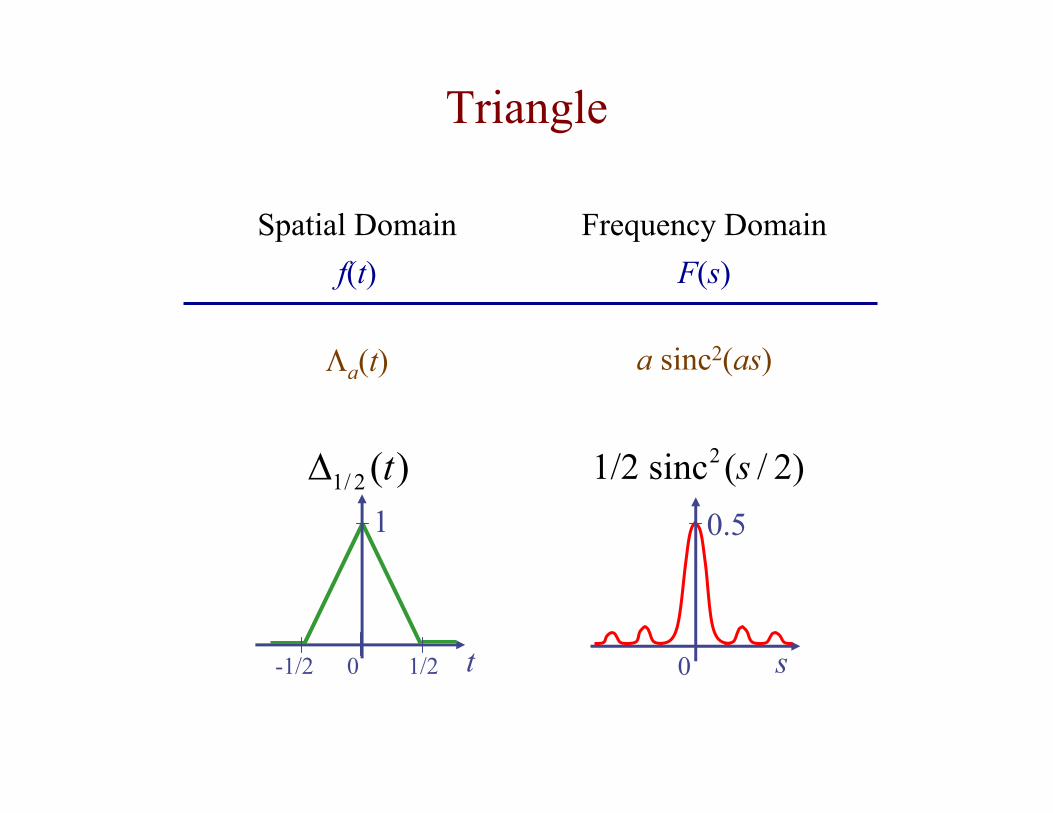
Triangle

a sinc2(as)Λa(t)

Frequency DomainF(s)

Spatial Domainf(t)

t0

1/ 2 ( )t∆1

1/2-1/2 s0

21/2 sinc ( / 2)s0.5

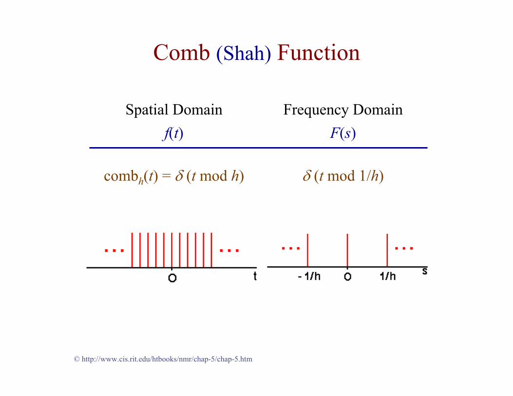
Comb (Shah) Function

δ (t mod 1/h)combh(t) = δ (t mod h)

Frequency DomainF(s)

Spatial Domainf(t)

© http://www.cis.rit.edu/htbooks/nmr/chap-5/chap-5.htm

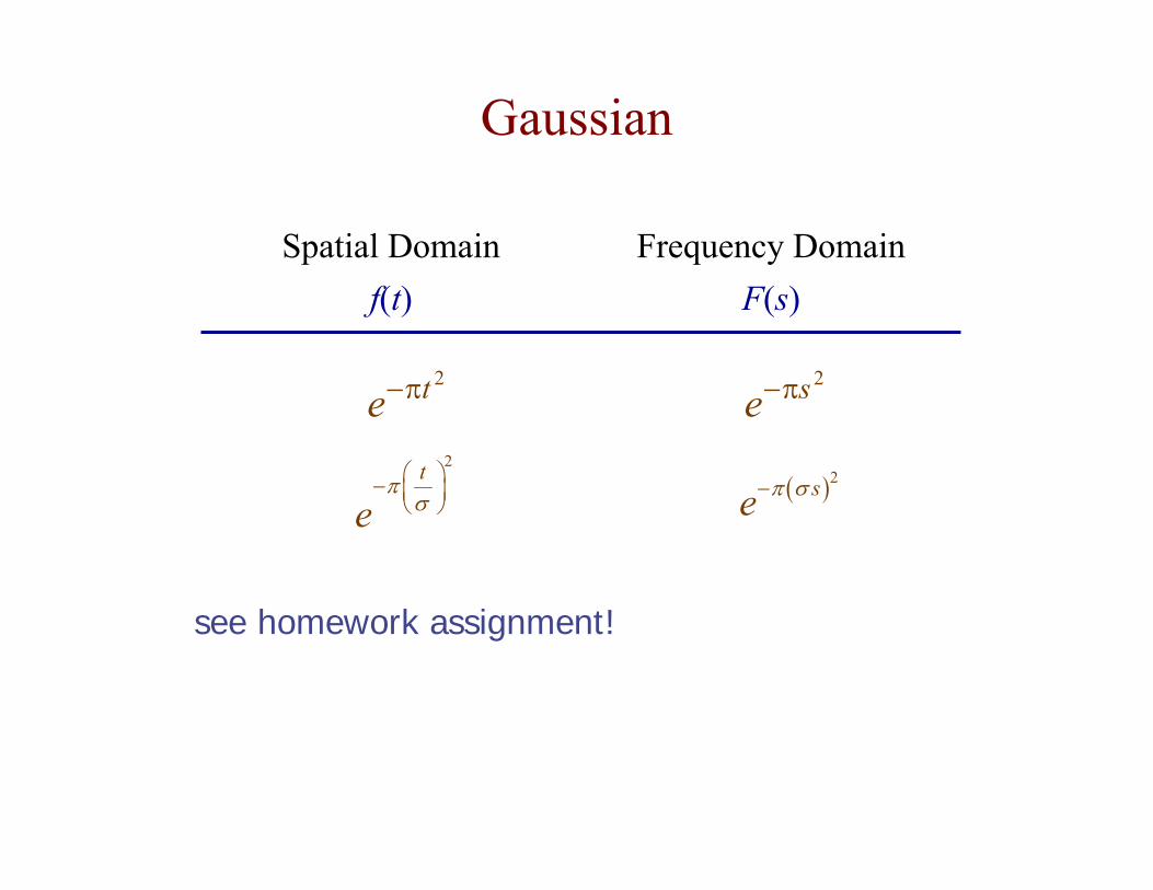
Gaussian

Frequency DomainF(s)

Spatial Domainf(t)

2se π−2te π−

( )2se π σ−2t

eπ

σ⎛ ⎞− ⎜ ⎟⎝ ⎠

see homework assignment!

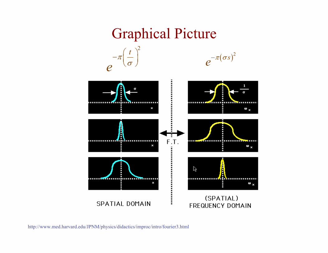
Graphical Picture

http://www.med.harvard.edu/JPNM/physics/didactics/improc/intro/fourier3.html

( )2se π σ−2t

eπ

σ⎛ ⎞− ⎜ ⎟⎝ ⎠

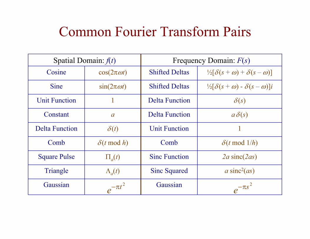
Common Fourier Transform Pairs

2a sinc(2as)Sinc FunctionΠa(t)Square Pulse

a sinc2(as)Sinc SquaredΛa(t)Triangle

GaussianGaussian

1Unit Functionδ (t)Delta Function

δ (t mod 1/h)Combδ (t mod h)Comb

Delta Function

Delta Function

Shifted Deltas

Shifted Deltas

Constant

Unit Function

Sine

Cosine ½[δ (s + ω) + δ (s – ω)]cos(2πωt)

½[δ (s + ω) - δ (s – ω)]isin(2πωt)

δ (s)1

a δ (s)a

Frequency Domain: F(s)Spatial Domain: f(t)

2se π−2te π−

FT Properties: Addition TheoremAdding two functions together adds their Fourier Transforms:

F(f + g) = F(f) + F(g)

Multiplying a function by a scalar constant multiplies its Fourier Transform by the same constant:

F(a f) = aF(f)

Consequence: Fourier Transform is a linear transformation!

FT Properties: Shift TheoremTranslating (shifting) a function leaves the magnitude unchanged and adds a constant to the phase

If f2(t) = f1(t – a)

F1 = F(f1) F2 = F(f2)

then|F2| = |F1|

φ (F2) = φ (F1) - 2πsa

Intuition: magnitude tells you “how much”,phase tells you “where”

FT Properties: Similarity TheoremScaling a function’s abscissa (domain or horizontal axis) inversely scales the both magnitude and abscissa of the Fourier transform.

If f2(t) = f1(a t)

F1 = F(f1) F2 = F(f2)

thenF2(s) = (1/|a|) F1(s / a)

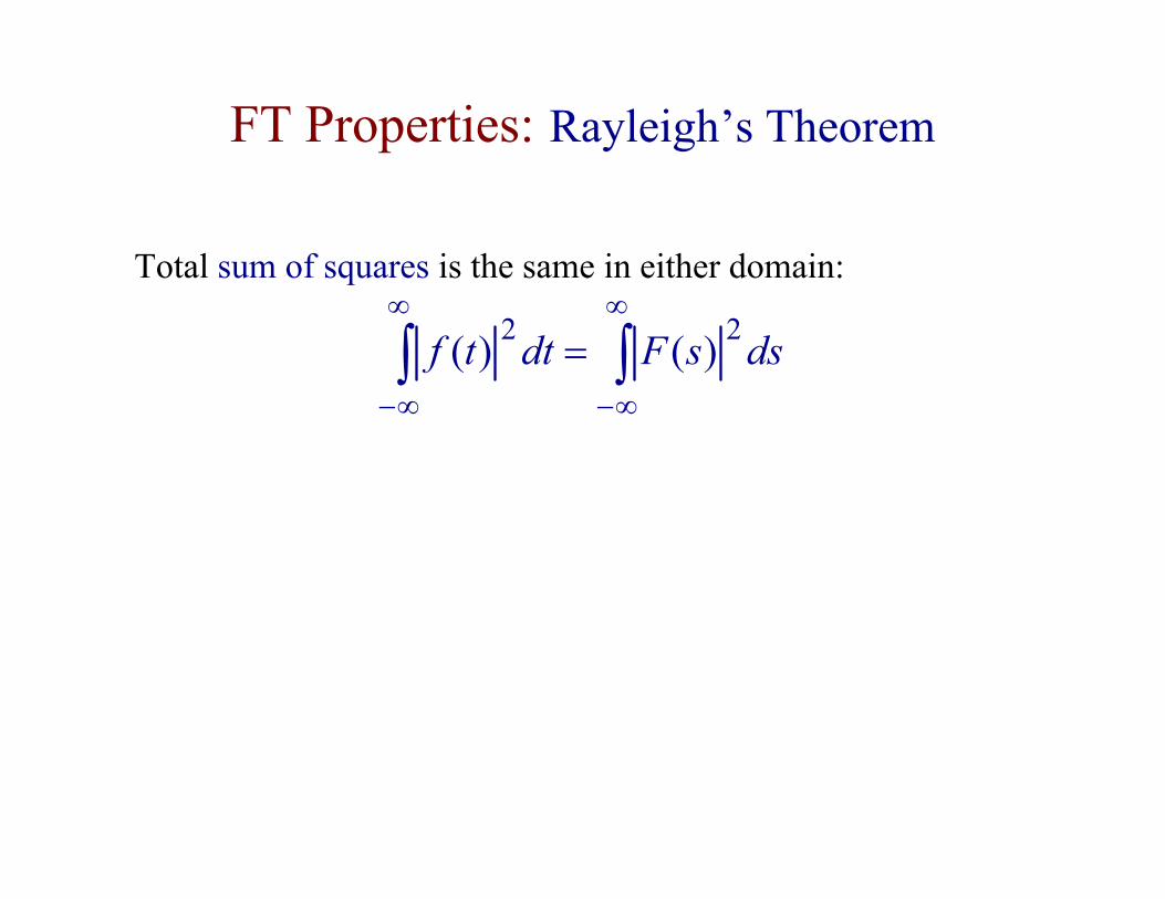
FT Properties: Rayleigh’s Theorem

Total sum of squares is the same in either domain:

∫∫∞

∞−

∞

∞−

= dssFdttf 22 )()(

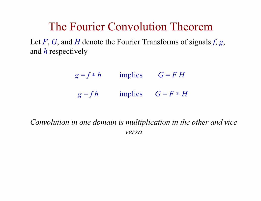
The Fourier Convolution TheoremLet F, G, and H denote the Fourier Transforms of signals f, g, and h respectively

g = f * h implies G = F H

g = f h implies G = F * H

Convolution in one domain is multiplication in the other and vice versa

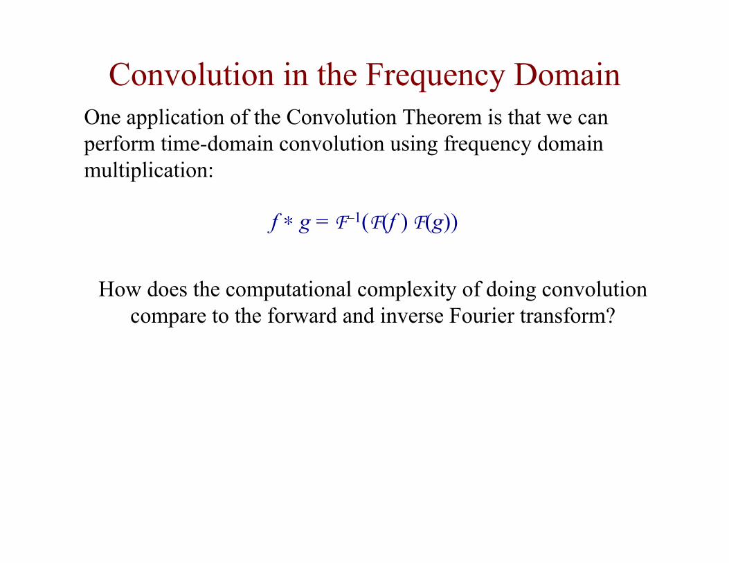
Convolution in the Frequency DomainOne application of the Convolution Theorem is that we can perform time-domain convolution using frequency domain multiplication:

f * g = F–1(F(f ) F(g))

How does the computational complexity of doing convolution compare to the forward and inverse Fourier transform?

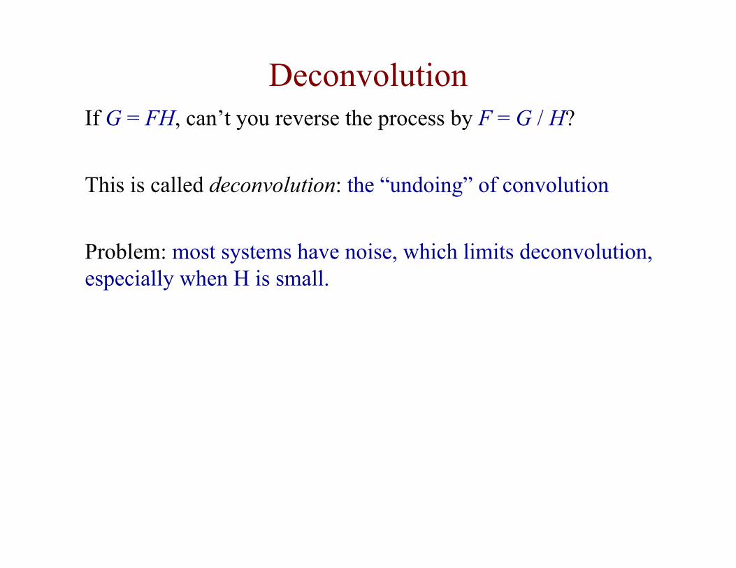
DeconvolutionIf G = FH, can’t you reverse the process by F = G / H?

This is called deconvolution: the “undoing” of convolution

Problem: most systems have noise, which limits deconvolution, especially when H is small.

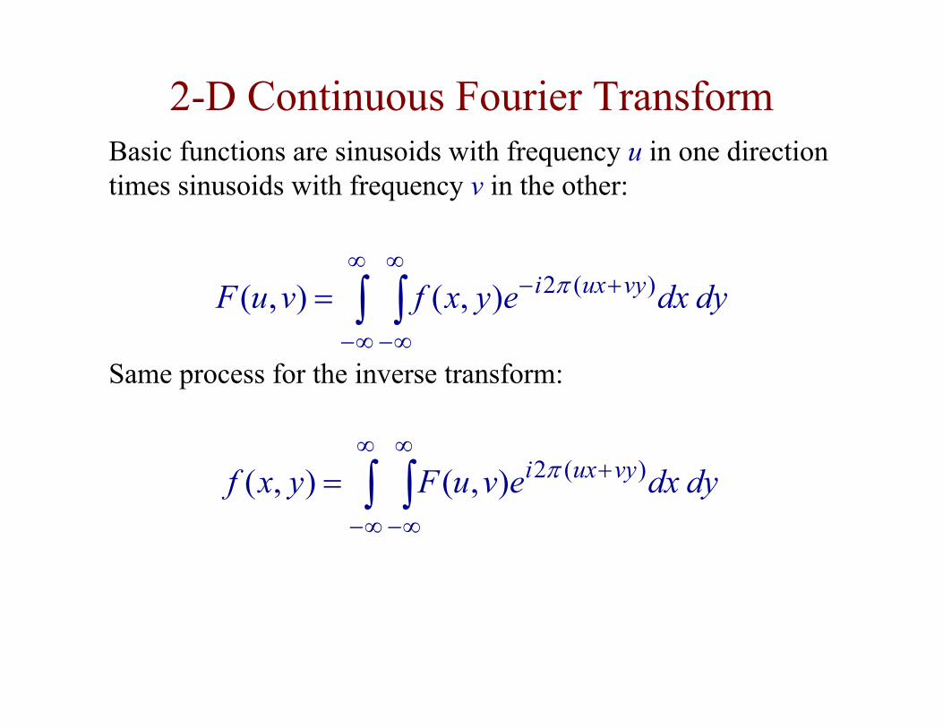
2-D Continuous Fourier TransformBasic functions are sinusoids with frequency u in one direction times sinusoids with frequency v in the other:

Same process for the inverse transform:

∫ ∫∞

∞−

∞

∞−

+−= dydxeyxfvuF vyuxi ),(),( )(2π

∫ ∫∞

∞−

∞

∞−

+= dydxevuFyxf vyuxi ),(),( )(2π

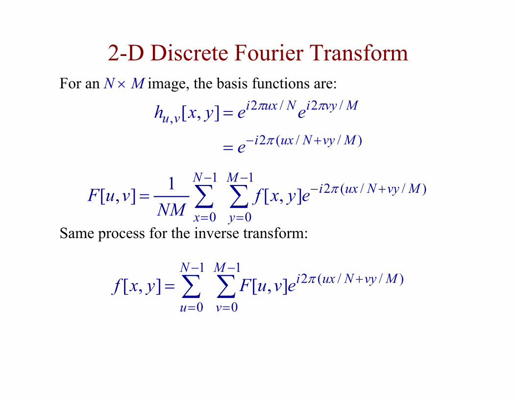
2-D Discrete Fourier TransformFor an N × M image, the basis functions are:

Same process for the inverse transform:

∑ ∑−

=

−

=

+=1

0

1

0

)//(2],[ ],[N

u

M

v

MvyNuxievuFyxf π

∑ ∑−

=

−

=

+−=1

0

1

0

)//(2],[ 1],[N

x

M

y

MvyNuxieyxfNM

vuF π

)//(2

/2/2, ],[

MvyNuxi

MvyiNuxivu

e

eeyxh+−=

=π

ππ

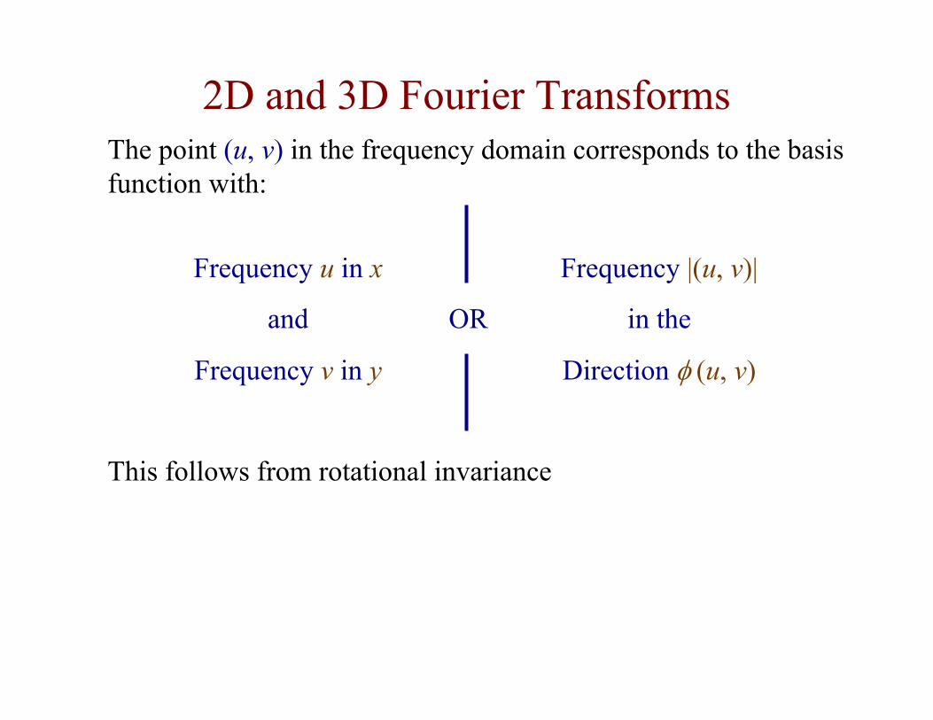
2D and 3D Fourier TransformsThe point (u, v) in the frequency domain corresponds to the basis function with:

Frequency u in x Frequency |(u, v)|

and OR in the

Frequency v in y Direction φ (u, v)

This follows from rotational invariance

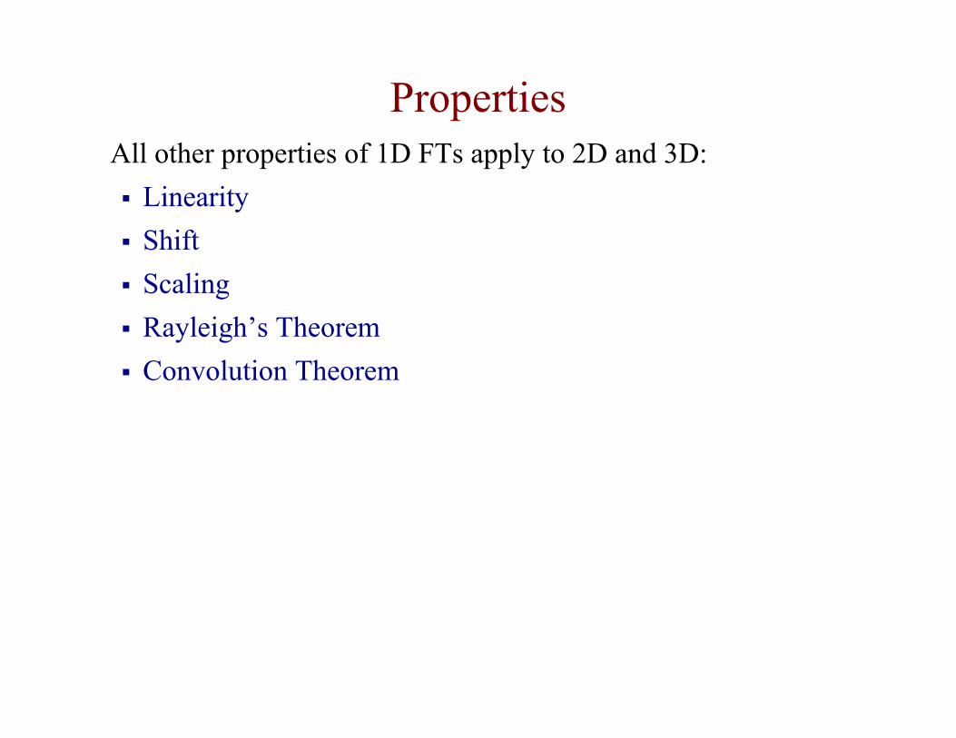
PropertiesAll other properties of 1D FTs apply to 2D and 3D:

LinearityShiftScalingRayleigh’s TheoremConvolution Theorem

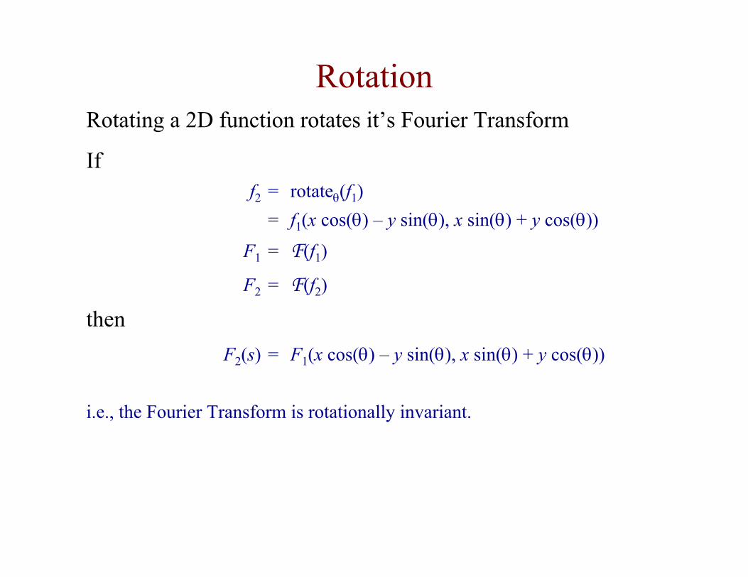
RotationRotating a 2D function rotates it’s Fourier Transform

Iff2 = rotateθ(f1)

= f1(x cos(θ) – y sin(θ), x sin(θ) + y cos(θ))

F1 = F(f1)

F2 = F(f2)

thenF2(s) = F1(x cos(θ) – y sin(θ), x sin(θ) + y cos(θ))

i.e., the Fourier Transform is rotationally invariant.

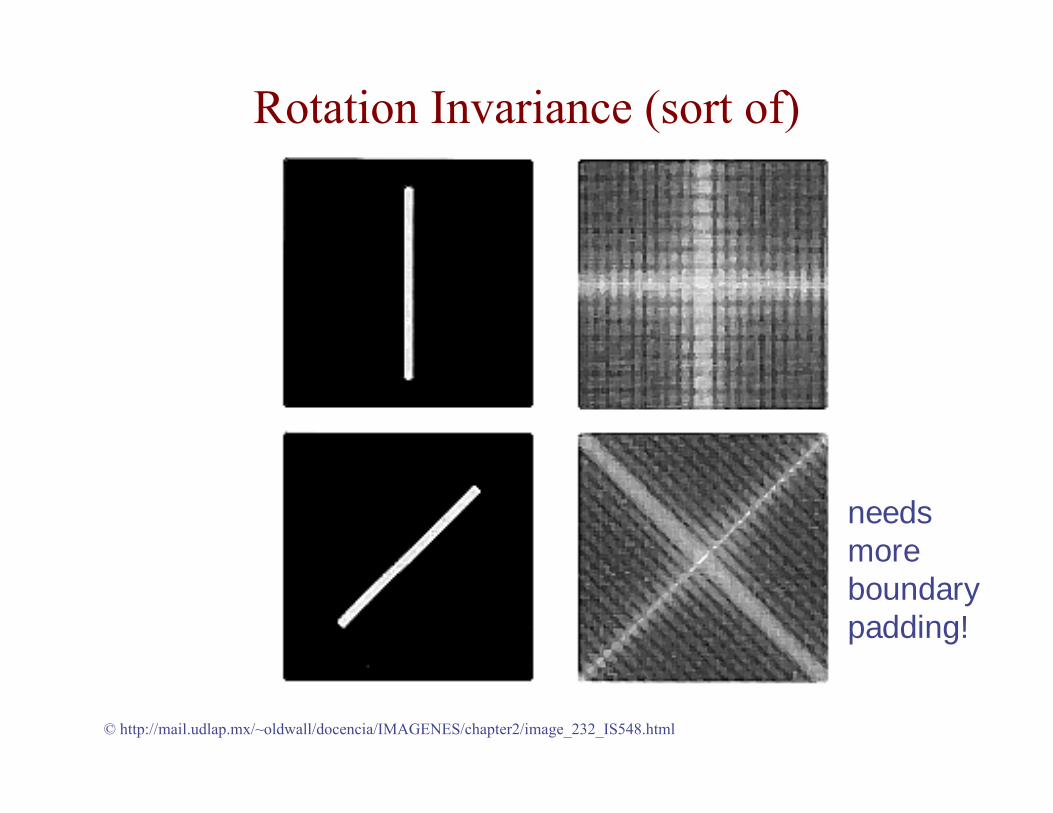
Rotation Invariance (sort of)

© http://mail.udlap.mx/~oldwall/docencia/IMAGENES/chapter2/image_232_IS548.html

needsmoreboundarypadding!

Transforms of Separable FunctionsIf

f(x, y) = f1(x) f2(y)

the function f is separable and its Fourier Transform is also separable:

F(u,v) = F1(u) F2(v)

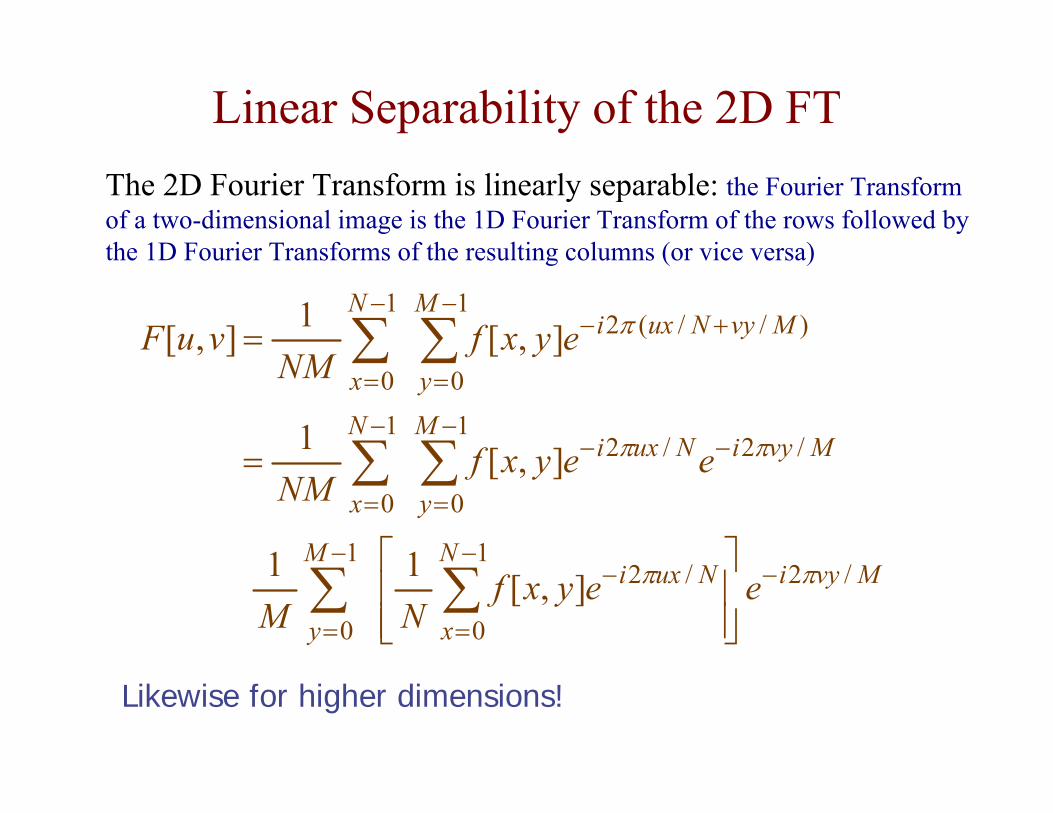
Linear Separability of the 2D FTThe 2D Fourier Transform is linearly separable: the Fourier Transform of a two-dimensional image is the 1D Fourier Transform of the rows followed by the 1D Fourier Transforms of the resulting columns (or vice versa)

MvyiM

y

N

x

Nuxi

MvyiN

x

M

y

Nuxi

N

x

M

y

MvyNuxi

eeyxfNM

eeyxfNM

eyxfNM

vuF

/21

0

1

0

/2

/21

0

1

0

/2

1

0

1

0

)//(2

],[1 1

],[ 1

],[ 1],[

ππ

ππ

π

−−

=

−

=

−

−−

=

−

=

−

−

=

−

=

+−

∑ ∑

∑ ∑

∑ ∑

⎥⎥⎦

⎤

⎢⎢⎣

⎡

=

=

Likewise for higher dimensions!

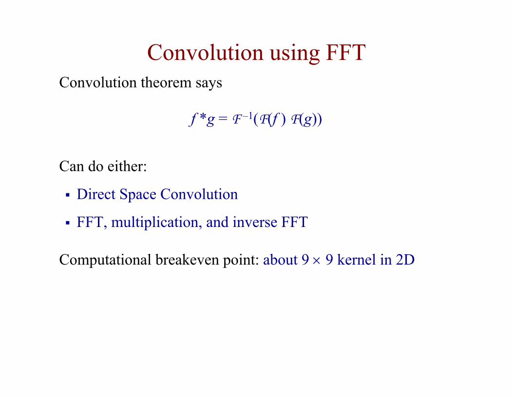
Convolution using FFTConvolution theorem says

f *g = F –1(F(f ) F(g))

Can do either:

Direct Space Convolution

FFT, multiplication, and inverse FFT

Computational breakeven point: about 9 × 9 kernel in 2D

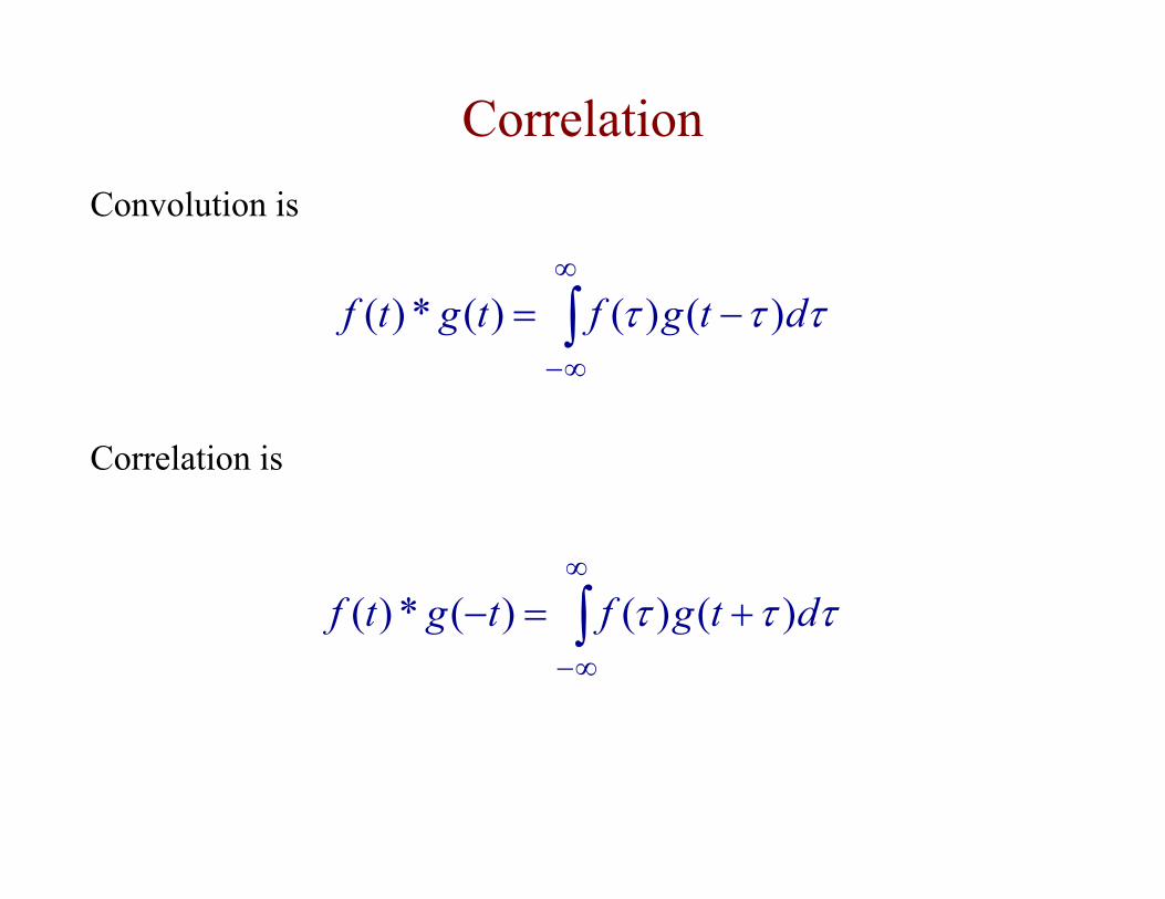
CorrelationConvolution is

Correlation is

∫∞

∞−

−= τττ dtgftgtf )()()( * )(

∫∞

∞−

+=− τττ dtgftgtf )()()( * )(

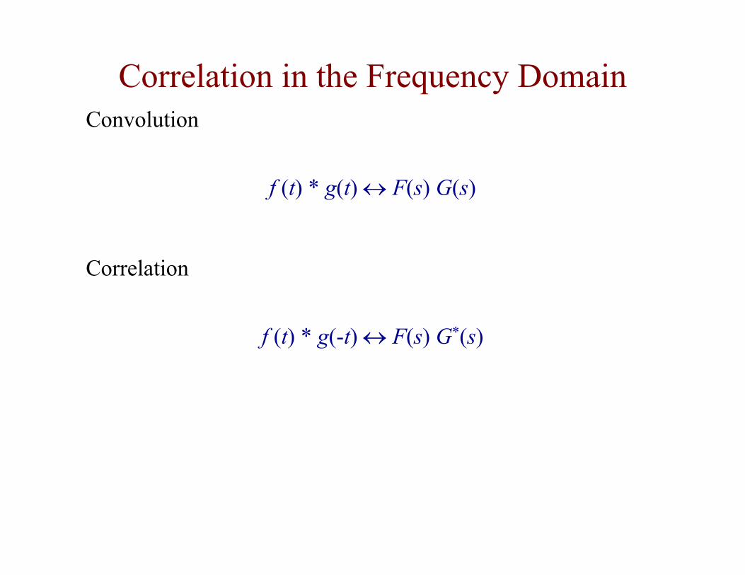
Correlation in the Frequency DomainConvolution

f (t) * g(t) ↔ F(s) G(s)

Correlation

f (t) * g(-t) ↔ F(s) G*(s)

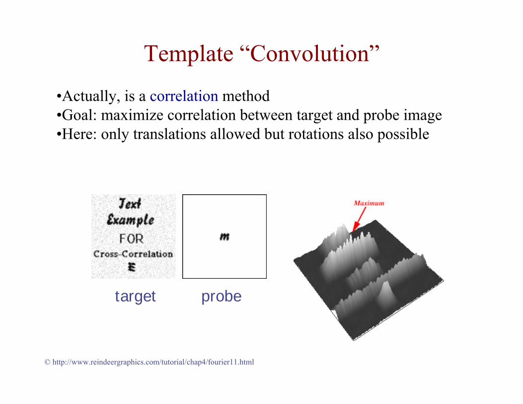
Template “Convolution”

•Actually, is a correlation method•Goal: maximize correlation between target and probe image•Here: only translations allowed but rotations also possible

target probe

© http://www.reindeergraphics.com/tutorial/chap4/fourier11.html

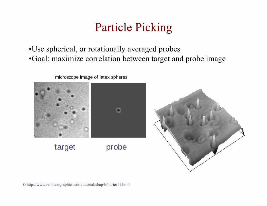
Particle Picking

•Use spherical, or rotationally averaged probes•Goal: maximize correlation between target and probe image

target probe

microscope image of latex spheres

© http://www.reindeergraphics.com/tutorial/chap4/fourier11.html

AutocorrelationAutocorrelation is the correlation of a function with itself:

f (t) * f(-t)

Useful to detect self-similarities or repetitions / symmetry within one image!

Power SpectrumThe power spectrum of a signal is the Fourier Transform of its autocorrelation function:

P(s) = F(f (t) * f (-t))

= F(s) F*(s)

= |F(s)|2

It is also the squared magnitude of the Fourier transform of thefunction

It is entirely real (no imaginary part).

Useful for detecting periodic patterns / texture in the image.

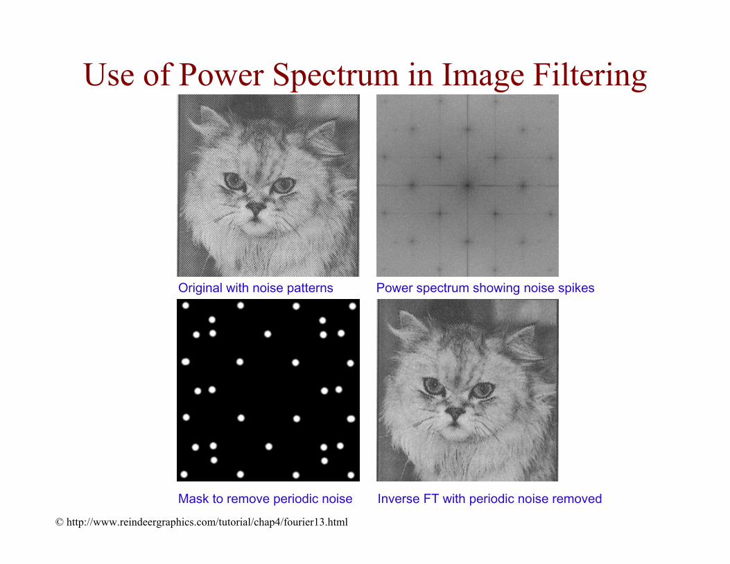
Use of Power Spectrum in Image Filtering

Original with noise patterns Power spectrum showing noise spikes

Mask to remove periodic noise Inverse FT with periodic noise removed© http://www.reindeergraphics.com/tutorial/chap4/fourier13.html

Figure and Text Credits

Text and figures for this lecture were adapted in part from the following source, in agreement with the listed copyright statements:

http://web.engr.oregonstate.edu/~enm/cs519© 2003 School of Electrical Engineering and Computer Science, Oregon State University, Dearborn Hall, Corvallis, Oregon, 97331

Resources

Textbooks:Kenneth R. Castleman, Digital Image Processing, Chapters 9,10John C. Russ, The Image Processing Handbook, Chapter 5