Embed Size (px)
Citation preview

Computational Mechanics Research and Support for Aerodynamics and Hydraulics at TFHRC, Year 1 Quarter 3 Progress Report
ANL/ESD/11-39
Energy Systems Division

Availability of This ReportThis report is available, at no cost, at http://www.osti.gov/bridge. It is also available on paper to the U.S. Department of Energy and its contractors, for a processing fee, from: U.S. Department of Energy OfficeofScientificandTechnicalInformation P.O. Box 62 Oak Ridge, TN 37831-0062 phone (865) 576-8401 fax (865) 576-5728 [email protected]
DisclaimerThis report was prepared as an account of work sponsored by an agency of the United States Government. Neither the United States Governmentnoranyagencythereof,norUChicagoArgonne,LLC,noranyoftheiremployeesorofficers,makesanywarranty,expressor implied, or assumes any legal liability or responsibility for the accuracy, completeness, or usefulness of any information, apparatus, product,orprocessdisclosed,orrepresentsthatitsusewouldnotinfringeprivatelyownedrights.Referencehereintoanyspecific commercial product, process, or service by trade name, trademark, manufacturer, or otherwise, does not necessarily constitute or imply its endorsement, recommendation, or favoring by the United States Government or any agency thereof. The views and opinions of documentauthorsexpressedhereindonotnecessarilystateorreflectthoseoftheUnitedStatesGovernmentoranyagencythereof,Argonne National Laboratory, or UChicago Argonne, LLC.
About Argonne National Laboratory Argonne is a U.S. Department of Energy laboratory managed by UChicago Argonne, LLC under contract DE-AC02-06CH11357. The Laboratory’s main facility is outside Chicago, at 9700 South Cass Avenue, Argonne, Illinois 60439. For information about Argonne and its pioneering science and technology programs, see www.anl.gov.

Computational Mechanics Research and Support for Aerodynamics and Hydraulics at TFHRC, Year 1 Quarter 3 Progress Report
ANL/ESD/11-39
byS.A. Lottes, R.F. Kulak, and C. BojanowskiTransportation Research and Analysis Computing Center (TRACC)Energy Systems Division, Argonne National Laboratory
August 2011
Computational Mechanics
Research and Support
for Aerodynamics and Hydraulics
at TFHRC
Quarterly Report
April through June 2011 Y1Q3

Computational Mechanics Research and Support
for Aerodynamics and Hydraulics at TFHRC
Year 1 Quarter 3 Progress Report
Energy Systems Division (ES)
Argonne National Laboratory (ANL)
Principal Investigators:
Steven A. Lottes, Ph.D.
Ronald F Kulak, Ph.D., PE, FASME
Contributor:
Cezary Bojanowski, Ph.D.
Submitted to:
Federal Highway Administration
Kornel Kerenyi, Ph.D. Turner-Fairbank Highway Research Center
Federal Highway Administration 6300 Georgetown Pike
McLean, VA 22101
Harold Bosch, Ph.D. Turner-Fairbank Highway Research Center
Federal Highway Administration 6300 Georgetown Pike
McLean, VA 22101
August, 2011

Table of Contents
1. Introduction and Objectives ................................................................................................................. 8
1.1. Computational Fluid Dynamics Summary ........................................................................................ 8
1.2. Computational Multiphyics Mechanics Summary ........................................................................... 9
2. Computational Fluid Dynamics for Hydraulic and Aerodynamic Research ........................................ 11
2.1. Entrainment Functions for RANS Scour Models and Tests of Alternatives ................................... 11
2.2. Initial Test of Mesh Morphing Applied to Transient Clear Water Pressure Flow Scour ................ 13
2.2.1. References .......................................................................................................................... 16
2.3. Computational Modeling and Analysis of Flow through Large Culverts for Fish Passage ............. 16
2.3.1. Model of Culvert Section with Fully Developed Flow Using Cyclic Boundary Conditions .. 18
2.3.2. Mesh Refinement Study ...................................................................................................... 19
2.3.3. Simulation Results and Discussion ...................................................................................... 22
2.3.4. Three Dimensional Model of Culvert Flume with Comparison to Experimental Results ... 30
2.3.5. Flow Conditions ................................................................................................................... 31
2.3.6. Results Using VOF Multiphase Model ................................................................................. 32
2.3.7. Comparison with the Single Phase Model .......................................................................... 33
2.3.8. Comparison with Laboratory Data ...................................................................................... 34
2.3.9. References .......................................................................................................................... 39
3. Computational Multiphysics Mechanics Applications ........................................................................ 40
3.1. Multiphysics Simulation of Salt Spray Transport ........................................................................... 40
3.1.1. Estimate for Water Content in Semi-Trailer Truck’s Wake ................................................. 40
3.1.2. Simulation of a Semi-trailer Truck Passing Through a Bridge Underpass ........................... 44
3.2. Wind Engineering ........................................................................................................................... 52
3.2.1. Vehicle Stability under High Wind Loadings ....................................................................... 53
3.2.2. Electromagnetic Shock Absorber for Vehicle Stability under High Wind Conditions ......... 63
3.3. A Coupling of CFD and CSM Codes for Scour Shape Prediction..................................................... 68
3.3.1. Introduction ........................................................................................................................ 68
3.3.2. Scour Slope Stability Based on Soil Mechanics ................................................................... 69
3.3.3. Procedure Flowchart ........................................................................................................... 70

TRACC/TFHRC Y1Q3 Page 3
3.3.4. Simplifying Assumptions ..................................................................................................... 70
3.3.5. Example of Use of the Procedure ....................................................................................... 71

TRACC/TFHRC Y1Q3 Page 4
List of Figures
Figure 2.1: Initial bed shear profile along flume with flooded bridge deck at 3.83 m to 4.09 m .............. 13
Figure 2.2: Bed shear after scour hole has fully formed ............................................................................ 14
Figure 2.3: Development of scour hole depth for simulation (red) and experiment (blue) ....................... 14
Figure 2.4: Initial streamwise velocity distribution around bridge deck .................................................... 15
Figure 2.5: Final velocity distribution after scour around flooded bridge deck. ........................................ 16
Figure 2.6: Reduced symmetric section of the barrel considered from a trough to trough ..................... 18
Figure 2.7: Refined mesh area with respect to the base created using a volumetric control ................... 19
Figure 2.8: Mesh scenes of the various cases used for mesh refinement studies .................................... 20
Figure 2.9: Sectional planes created at the trough and the crest to resolve flow parameters ................. 21
Figure 2.10: Uniform strips created using “Thresholds” feature available in STAR-CCM+ ........................ 22
Figure 2.11: Surface averaged velocity vs. length of the plane section (created at a trough) plot for
meshes 1-3 .................................................................................................................................................. 23
Figure 2.12: Surface averaged velocity vs. length of the plane section (created at a trough) plot for
meshes 4-6 .................................................................................................................................................. 24
Figure 2.13: Line probes created at a trough and a crest along the flow field in the reduced barrel ....... 25
Figure 2.14: Velocity profiles of the different mesh cases with base size as 10mm plotted at a crest ..... 25
Figure 2.15: Velocity profiles of the different mesh cases with base size 5mm plotted at a crest ........... 26
Figure 2.16: Velocity profiles of the different mesh cases with base size 10mm plotted at a trough ...... 27
Figure 2.17: Velocity profiles of the different mesh cases with base size 5 mm plotted using at a trough
.................................................................................................................................................................... 28
Figure 2.18: Velocity plots of the various mesh cases in the mesh refinement study .............................. 29
Figure 2.19: Three-dimensional CAD model for multi-phase simulations ................................................. 30
Figure 2.20: Dimensional details of the flume (front and top views) ........................................................ 31
Figure 2.21: Velocity distribution across trough section of the multi-phase model for 3 inch water depth
.................................................................................................................................................................... 32

TRACC/TFHRC Y1Q3 Page 5
Figure 2.22: Velocity distribution across trough section of the multi-phase model for 6 inch water depth
.................................................................................................................................................................... 33
Figure 2.23: Velocity distribution across trough section of the multi-phase model for 9 inch water depth
.................................................................................................................................................................... 33
Figure 2.24: Multi-phase model vs. full flume single phase model illustrating velocity distribution across
trough section for 6 inch water depth ........................................................................................................ 34
Figure 2.25: CFD velocity contour plot with ADV cut area (upper) vs. ADV velocity contour plot (lower)
for 6 inch water depth on the trough section ............................................................................................ 35
Figure 2.26: CFD velocity contour plot with PIV cut area (upper) vs. PIV velocity contour plot (lower) for
6 inch water depth on the trough section .................................................................................................. 36
Figure 2.27: CFD velocity contour plot with ADV cut area (upper) vs. ADV velocity contour plot (lower)
for 9 inch water depth on the trough section ............................................................................................ 37
Figure 2.28: 90% single phase CFD velocity contour plot with PIV cut area from (upper) vs. PIV velocity
contour plot (lower) for 6 inch water depth on the trough section ........................................................... 38
Figure 3.1: Egression of the salt-water air mixture into the air outside of the vehicle forming two side-of-
vehicle clouds and a rear undercarriage cloud [1] ...................................................................................... 40
Figure 3.2: Setup for analysis of the air movement under the bridge ........................................................ 44
Figure 3.3: Behavior of tracer particles at the level of the wheel axis ....................................................... 46
Figure 3.4: Behavior of tracer particles at the level of the engine hood .................................................... 47
Figure 3.5: Behavior of tracer particles at the level of the windshield ....................................................... 48
Figure 3.6: Behavior of tracer particles at the level of the top surface of the trailer ................................. 49
Figure 3.7: Close up view of the velocity vectors ....................................................................................... 50
Figure 3.8: Velocity vectors in the middle cross section of the air domain ................................................ 51
Figure 3.9: Single unit rigid vehicle [1] ........................................................................................................ 59
Figure 3.10: Mass-less nodes moving on a beam element ......................................................................... 59
Figure 3.11: Motion of block attached with spring elements ..................................................................... 60
Figure 3.12: Wind loading applied at the side of the block ........................................................................ 60
Figure 3.13: Displacement graph of block model with vertical springs and horizontal load ...................... 60
Figure 3.14: FEM Model of a Ford F-800 truck obtained from NCAC [2] .................................................... 61
TRACC/TFHRC Y1Q3 Page 6
Figure 3.15: FEM model modified according to the analysis ...................................................................... 61
Figure 3.16: Graph of free displacement of truck on the suspension ........................................................ 62
Figure 3.17: Displacement graph of various damped values ...................................................................... 62
Figure 3.18: Plot of the Desired Force, based upon the states ................................................................... 64
Figure 3.19: Plot of the EMSA force ............................................................................................................ 65
Figure 3.20: Schematic of the road profile data ......................................................................................... 65
Figure 3.21: Actual road profile plot ........................................................................................................... 66
Figure 3.22: Plot of reaction force vs. the prescribed motion .................................................................... 67
Figure 3.23: Plot of force vs. displacement, for displacements less than 15 mm ...................................... 68
Figure 3.24 Strength envelope in terms of yield surface- second invariant of deviatoric stress and
pressure ...................................................................................................................................................... 70
Figure 3.25 Initial scour shape based on STAR-CCM+ calculation .............................................................. 71
Figure 3.26 Finite Element model of the scour hole – initial state ............................................................. 72
Figure 3.27 Finite Element model of the scour hole – final state ............................................................... 72
Figure 3.28 Comparison of the initial and the final shape of the scour hole ............................................. 73

TRACC/TFHRC Y1Q3 Page 7
List of Tables
Table 2.1: Boundary conditions ................................................................................................................. 18
Table 2.2: Details of the various meshes used in the mesh refinement study .......................................... 21
Table 2.3: Flow conditions ......................................................................................................................... 32
Table 3.1: Water content in sampling domain generated by a GCM traveling at 29 m/s (65 mph) [1] ..... 41
Table 3.2: Cloud material densities generated by a GCM traveling at 29 m/s (65 mph) ........................... 42
Table 3.3 Statistics of the FE model of the bridge ...................................................................................... 44
Table 3.4 RMS value comparison between passive and active systems .................................................... 66
Table 3.5 Total mass values for F800 truck model ..................................................................................... 66

TRACC/TFHRC Y1Q3 Page 8
1. Introduction and Objectives
The computational fluid dynamics (CFD) and computational structural mechanics (CSM) focus areas at
Argonne’s Transportation Research and Analysis Computing Center (TRACC) initiated a project to
support and compliment the experimental programs at the Turner-Fairbank Highway Research Center
(TFHRC) with high performance computing based analysis capabilities in August 2010. The project was
established with a new interagency agreement between the Department of Energy and the Department
of Transportation to provide collaborative research, development, and benchmarking of advanced
three-dimensional computational mechanics analysis methods to the aerodynamics and hydraulics
laboratories at TFHRC for a period of five years, beginning in October 2010. The analysis methods
employ well-benchmarked and supported commercial computational mechanics software.
Computational mechanics encompasses the areas of Computational Fluid Dynamics (CFD),
Computational Wind Engineering (CWE), Computational Structural Mechanics (CSM), and Computational
Multiphysics Mechanics (CMM) applied in Fluid-Structure Interaction (FSI) problems.
The major areas of focus of the project are wind and water loads on bridges — superstructure, deck,
cables, and substructure (including soil), primarily during storms and flood events — and the risks that
these loads pose to structural failure. For flood events at bridges, another major focus of the work is
assessment of the risk to bridges caused by scour of stream and riverbed material away from the
foundations of a bridge. Other areas of current research include modeling of flow through culverts to
assess them for fish passage, modeling of the salt spray transport into bridge girders to address
suitability of using weathering steel in bridges, vehicle stability under high wind loading, and the use of
electromagnetic shock absorbers to improve vehicle stability under high wind conditions.
This quarterly report documents technical progress on the project tasks for the period of April through
June 2011.
1.1. Computational Fluid Dynamics Summary
The primary Computational Fluid Dynamics (CFD) activities during the quarter concentrated on the
development of models and methods needed to complete the next steps in scour and culvert modeling.
Work on identifying and fitting a sediment entrainment function to model transient pressure flow scour

TRACC/TFHRC Y1Q3 Page 9
experiments at TFHRC continued. A methodology to use transient CFD scour analysis itself to iteratively
refine entrainment function parameters to match experimental results is proposed. Using the CFD
software to tune empirical functions for the scour physics models is expected to produce more robust
models for CFD analysis than those that are determined outside of the CFD framework. Work reported
under the USDOT Y5Q3 report has been nearly completed on scour model enhancements needed to
displace the bed in a direction normal to the bed instead of simply vertically, to account for the effect of
bed slope on the scour rate, and to include a simple sand slide model to keep the bed slope less than or
equal to the angle of repose of the sediment. These scour model enhancements will be incorporated
into future scour modeling work.
Culvert analysis focused on determination of detailed velocity distributions to improve design
procedures for culverts that need to allow for fish passage continued. A mesh refinement study for
22.86 cm (9 inch) flow depth cases was completed, and a 5 mm base mesh size with a 67% refinement in
the corrugated region is recommended for CFD analysis of these cases in the TFHRC culvert test matrix.
In another study, culvert modeling results were compared to experimental data obtained in two ways
using Particle Image Velocimetry (PIV) and Acoustic Doppler Velocimetry (ADV). Differences between
modeling results were within the range obtained with the two experimental methods and the results
appear to be good enough to use for engineering analysis of culvert flow to improve the design
procedures that allow for fish passage under low flow conditions.
1.2. Computational Multiphyics Mechanics Summary
Computational Multiphysics Mechanics Research for Turner-Fairbank Highway Research Center
continued in the following four areas: (1) multiphysics simulation of salt spray transport; (2) simulation
of a semi-trailer truck passing through a bridge underpass; (3) vehicle stability under high wind loadings;
and (4) electromagnetic shock absorber for vehicle stability under high wind conditions. In Area 1, a
literature search identified previous research performed at Lawrence Livermore National Laboratory
from which estimates of the spatial distribution of the salt spray created by truck tires and the resulting
density of the airborne salt water cloud behind the truck were extracted.
In Area 2, simulations were performed to study the motion of air as a semi-trailer truck approaches and
passes through a bridge underpass and, in particular, to evaluate the transport of tire-generated salt
spray onto the underside of bridges made from weathering steel. Marker particles at several levels
above the roadbed were identified in the model and their motion as the truck approached and passed
through the underpass was studied. In the direction of vehicle travel, only the particles near the top of
the truck were found to reach the lower portions of the bridge support beams. This implies that should
salt-laden air be at this level – which is implied from the Livermore research – then the salt spray could
reach at least the flange level of the support beams. In the direction perpendicular to travel, it was
found that as the truck approaches, the air from the roadway is pushed into the space between the
beams, and as the truck exits, the air reverses direction and tends to move into the space vacated by the
truck. TRACC staff and NIU staff (professor/student) continued working on two Wind Engineering
projects.
TRACC/TFHRC Y1Q3 Page 10
The Area 3 work deals with the effects of wind loading on vehicles to evaluate rollover potential. A finite
element model of a Ford F-800 truck was downloaded from the National Crash Analysis Center (NCAC).
A wind pressure loading was applied to the one side of the truck, and studies on the resulting dynamic
response have begun.
The Area 4 work is the development of an electromagnetic shock absorber control algorithm that can
increase the stability of trucks driving in high wind conditions. New work done during the third quarter
involved the analytical modeling of the electromagnetic shock absorber as well as its incorporation into
the ¼ car Simulink model; the Simulink model utilizes an actual road profile as the disturbance for the
system and the data is automatically exported into Microsoft Excel for post-processing. Also, finite
element simulations of the Ford F800 truck model were performed to obtain mass, stiffness and
damping properties.

TRACC/TFHRC Y1Q3 Page 11
2. Computational Fluid Dynamics for Hydraulic and Aerodynamic Research
The effort during the third quarter continued developing an approach to obtaining a good sediment
entrainment rate function for pressure flow scour and continued development of methods for enhanced
analysis of culvert flow for fish passage that account for the velocity distribution over a cross section.
2.1. Entrainment Functions for RANS Scour Models and Tests of Alternatives
Guo’s [2] empirical formula for bed recession rate at the deepest point were used as the basis for
obtaining a bed recession rate field function to morph the bed at any point on the bed as a function of
the local shear stress. The formula was based on transient scouring experiments run at TFHRC and is
given by:
( )
(2.1)
where Y is dimensionless time-dependent scour depth, defined as /ys in which is the maximum
depth of the scour hole at a given time and ys is the final depth of the scour hole. T is dimensionless
time, defined as tVu/hb where Vu is upstream velocity and hb is height of the bottom of the bridge deck
above the upstream (unscoured) bed. Tc = 1.56 X 10⁵ is a characteristic dimensionless time parameter
used to fit experimental data.
In terms of dimensional variables this becomes:
( ) (2.2)
where a = Vu/(hbTc).
Equation (2.2) can be solved for t to give the laboratory time at which the scour hole reaches depth y:

TRACC/TFHRC Y1Q3 Page 12
[ (
)
] (2.3)
Differentiating Equation (2.3) gives the bed recession rate at the point of maximum scour:
[ ]
(2.4)
One problem with this fitted function is that the bed recession rate approaches infinity at time zero,
which is physically unrealistic. The function fits the experimental data reasonably well after the first ½
hour, however, the actual bed recession rate at time zero in the TFHRC pressure flow scour experiments
is a finite value that is a small fraction of a meter per second. Because over one third of the final depth
of the scour hole may be reached in the first half hour, that time period is important in a CFD simulation
that starts from time zero with a flat bed. Currently alternatives for dealing with a lack of data for the
scour rate during the first half hour are being investigated.
Assuming that the entrainment rate is independent of time and a function of the local bed shear stress
and bed slope, then Equations (2.3) and (2.4) can be used to fit an entrainment rate that is a function of
shear stress at the point of maximum shear and that function can be applied anywhere on the bed.
Three candidate functions are proposed. One by Xie [4] has the form:
(2.5)
in which τm denotes the maximum bed shear stress. Eb denotes the recession rate or sediment pickup
rate. An initial fit yields the parameters: a = 2.933e-011, b = 4.034, c = -0.001206, d = -4.645. Initial
testing of this function fit found that the scour away from the point of greatest depth was too slow and did
not match the bed profiles at intermediate times.
The entrainment function by Van Rijn and a chemical kinetic rate law analogy proposed by Lottes [1]
have been considered, and initial testing of these model functions for clear water pressure flow scour
has begun. The Van Rijn function is a power law function of the form:
(
)
(2.6)
(2.7)
where Eb is the sediment pickup rate in units of mass per unit sediment bed area and per unit time,
kg/(m2 s). Initial tests using the constants given by Van Rijn yielded scour rates that were too fast and a
pressure flow scour hole that was too deep, two or more times the experimental scour depth.
The rate law as proposed by Lottes [1] has the form:

TRACC/TFHRC Y1Q3 Page 13
(
)
( ) (2.8)
where A0, A1, and n are fitting parameters. An initial fit of these parameters to the reduced
experimental results by Guo yields
( ) ( ) ( ) (2.9)
2.2. Initial Test of Mesh Morphing Applied to Transient Clear Water Pressure Flow
Scour
An initial simulation using the bed recession rate given by Equation (2.9) was performed. The initial bed
shear is shown in Figure 2.1. The bridge deck extends from 3.83 m to 4.09 m. The peak in shear is 9 cm
from the trailing edge of the deck. The lower peak near x = 0.0 is due to a honeycomb at the inlet that
straightens the flow, helps to ensure a uniform velocity across the flume, and strips off the boundary
layer at the bed. The reforming boundary layer generates locally high bed shear extending to
approximately x = 0.7 m. In that upstream zone the bed is fixed and cannot be eroded.
Figure 2.1: Initial bed shear profile along flume with flooded bridge deck at 3.83 m to 4.09 m
Figure 2.2 shows that the local peak in bed shear stress under the submerged bridge deck has dropped
as flow area under the deck is increased through the erosion of bed material to a plateau that is near
the critical value to initiate motion of stationary sediment particles on the bed.

TRACC/TFHRC Y1Q3 Page 14
Figure 2.2: Bed shear after scour hole has fully formed
Figure 2.3: Development of scour hole depth for simulation (red) and experiment (blue)
A transient plot of scour hole depth from a simulation using Equation (2.9) for the bed recession rate is
compared to the depth determined from Equation (2.2), which was derived by correlation with TFHRC
experimental data by Guo [6]. The simulation was run out to 380,000 s (102 hour) where the scour
depth from the simulation crosses the laboratory data fit. The experiment for the case was run for
151,200 s (42 hours). The rate function used in the simulation is too slow in the initial period, although
that is not apparent in the figure due to the long time scale, and it is faster than the laboratory rate
later, which allows it to eventually catch up. Figure 2.3 also shows a proposed procedure to iteratively

TRACC/TFHRC Y1Q3 Page 15
refine the rate function to improve the match to experimental results using the results of the CFD
simulation. The CFD simulation yields the bed shear at the current scour depth at each time step. The
laboratory time at which the simulated scour depth was reached can be computed from Equation (2.3),
for times greater than 1800 s. Also for times greater than 1800 s, the bed recession rate at the depth
from the simulation can be calculated from Equation (2.4). This procedure yields a new value for bed
recession rate corresponding to the bed shear at the maximum depth for each time step. These new
values can be used to improve the parameters for the entrainment rate function. As noted in Section
2.1, there are no experimental data for the first 1800 s, and the erosion rate at the deepest point as a
function of time, Equation (2.4) has a physically unrealistic singular point at time equal to zero. In the
absence of experimental data, some reasonable assumptions are needed to determine an erosion rate
as a function of bed shear during the first 1800 s that will result in the simulation matching the
experimental scour depth within the range of uncertainty at 1800 s. The procedure for achieving this
goal is currently under development.
The streamwise velocity distribution in the vicinity of the flooded bridge deck at the initial unscoured
state is shown in Figure 2.4. It clearly shows accelerated flow under the deck and a much higher velocity
near the bed than in the upstream. Figure 2.5 shows the streamwise velocity distribution after the scour
hole has fully formed. The accelerated flow under the deck is significantly reduced, and the near bed
boundary layer is thicker, which yields a reduced shear stress peak under the bed and near zero erosion
rate.
Figure 2.4: Initial streamwise velocity distribution around bridge deck

TRACC/TFHRC Y1Q3 Page 16
Figure 2.5: Final velocity distribution after scour around flooded bridge deck.
2.2.1. References
1. Lottes, S.A., Hydraulics and Scour Modeling Notes, unpublished, Argonne National
Laboratory, 2011.
2. Guo, Junke, Time-dependent scour of submerged bridge flows, paper in preparation,
Department of Civil Engineering University of Nebraska-Lincoln, 2011.
3. Guo, Junke, et.al., Bridge Pressure Flow Scour at Clear Water Threshold Condition, Trans.
Tianjin Univ., 2009, 15;079-094.
4. Xie, Z., Pressure Flow Scour Notes, unpublished, University of Nebraska.
2.3. Computational Modeling and Analysis of Flow through Large Culverts for Fish
Passage
Fish passage through culverts is an important component of road and stream crossing design. As water
runoff volume increases, the flow often actively degrades waterways at culverts and may interrupt
natural fish migration. Culverts are fixed structures that do not change with changing streams and may
instead become barriers to fish movement. The most common physical characteristics that create
barriers to fish passage include excessive water velocity, insufficient water depth, large outlet drop
heights, turbulence within the culvert, and accumulation of sediment and debris. Major hydraulic
criteria influencing fish passage are: flow rates during fish migration periods, fish species, roughness,
and the length and slope of the culvert.

TRACC/TFHRC Y1Q3 Page 17
The objective of this work is to develop approaches to CFD modeling of culvert flows and to use the
models to perform analysis to assess flow regions for fish passage under a variety of flow conditions.
The flow conditions to be tested with CFD analysis are defined in the tables of a work plan from TFHRC
[6]. The CFD models are being verified by comparing computational results with data from experiments
conducted at TFHRC. A primary goal of CFD analysis of culverts for fish passage is to determine the local
cross section velocities and flow distributions in corrugated culverts under varying flow conditions. In
order to evaluate the ability of fish to traverse corrugated culverts, the local average velocity in vertical
strips from the region adjacent to the culvert wall out to the centerline under low flow conditions will be
determined.
A primary goal of the CFD analysis during this quarter has been to determine the local velocities and
flow distributions through culverts for the fish passage with no gravel in the culvert. In order to more
accurately evaluate the ability of fish to traverse culverts, it is desirable to look at the changes in the
local average velocity of the flow adjacent to the culvert wall under low flow conditions. CFD runs using
the cyclic boundary conditions to obtain the fully developed flow on a reduced 3D section of the culvert
(symmetric quarter of the culvert section with corrugations from trough to another trough) have been
conducted using CD-adapco’s STAR-CCM+ software. Use of the cyclic boundary condition requires an
assumption of a nearly flat water surface that can be modeled with a symmetric boundary condition
that allows a free slip water velocity at that boundary. The cyclic boundary approach shortens the
simulation time required to establish a fully developed flow with a known mass flow rate (with this
approach several test cases can be completed per day). The periodic fully developed condition is
achieved by creating a cyclic boundary condition, where all outlet variables are mapped back to the inlet
interface, except for the pressure because there is a pressure drop corresponding to the energy losses in
the culvert section. The pressure jump needed to balance the pressure drop for the specified mass flow
is iteratively computed by the CFD solver. The runs were conducted with various mesh sizes, to take a
closer look at how the velocity distribution and other flow parameters vary at different locations of the
flow field by varying the base size of the mesh to obtain solutions that are effectively mesh
independent. The mesh refinement study is also used to identify meshes that are computationally
efficient while yielding good mesh independent results. An investigation of how the flow field varies for
different cases such as reduced culvert section when considered from a trough to trough versus crest to
crest. The computational model is based on the three-dimensional transient RANS k-epsilon turbulence
model with wall function treatment.
The modeling work was done in collaboration with staff at TFHRC conducting physical experiments of
culvert flows for the fish passage project in the Federal Highway Administration (FHWA). A preliminary
comparison of the velocity distribution on the trough section between CFD model results and laboratory
observation data was conducted. The 3D CFD model solves the Reynolds averaged Navier-Stokes (RANS)
equations with k-epsilon turbulence model with wall function. The VOF method, which captures the free
surface profile through use of the variable known as the volume of fluid was used in the multi-phase
CFD model. The verification of the CFD model for engineering application using the laboratory
observation data is a key step for the further work. A comparison of the multi-phase model and full scale
flume single phase model was also done.

TRACC/TFHRC Y1Q3 Page 18
2.3.1. Model of Culvert Section with Fully Developed Flow Using Cyclic Boundary Conditions
In this study, a simulation model was developed using the commercial CFD software STAR-CCM+. A
small section of the culvert barrel was modeled with cyclic boundaries at the inlet and outlet sections of
the computational domain. A 36 inch diameter culvert with corrugation size 3 inches by 1 inch has been
used for this study. The flow depth was 9 inches, a flow velocity was 0.71 feet/second, and zero bed
elevation in the culvert (no gravel present).
Figure 2.6: Reduced symmetric section of the barrel considered from a trough to trough
The boundary conditions used for the computational model in Figure 2.6 are listed in Table 2.1 below.
All the CFD runs have been carried out with the same set of boundary conditions.
Table 2.1: Boundary conditions
Boundary Name Type
Face at minimum x value Inlet Cyclic boundary condition
Face at maximum x value Outlet Cyclic boundary condition
Water surface Top Symmetry plane
Centerline Center Symmetry plane
all other surfaces Barrel No-slip wall

TRACC/TFHRC Y1Q3 Page 19
2.3.2. Mesh Refinement Study
As detailed in the previous quarterly report, a CFD procedure is being developed to test the flow
conditions that are defined in the tables of the work plan from TFHRC [6]. As a part of developing the
procedure, mesh refinement studies are being conducted for each geometry configuration in the work
plan. Sensitivity to mesh refinement will need to be checked for the larger culverts in the work plan
when the geometry for those culverts are built. In the process of mesh refinement various base sizes
have been chosen, along with the creation of a volumetric control (annulus ring) along the corrugated
section. The refinement of the mesh is defined by specifying a reduction of mesh size for volume within
an annulus intersecting the model as shown in Figure 2.7. The volumetric control body intersecting the
corrugated section provides a means to refine the mesh in the corrugated region of interest. The refined
mesh enables better resolution of the flow field with recirculation zones at the troughs between the
corrugations. Meshing also includes a prism layer consisting of orthogonal prismatic cells running
parallel to the wall boundaries, which constitutes a boundary mesh that is good for the application of
wall functions to compute the shear stress at the wall boundaries.
Figure 2.7: Refined mesh area with respect to the base created using a volumetric control
A volumetric control (annulus ring) was created intersecting the corrugated section to specially refine
the mesh around this region with respect to the base as shown in Figure 2.7. Figure 2.8 does not show a
coarser version of mesh 1 and mesh 4 because they look similar to mesh scenes 2 and 5 with larger cells.
Sensitivity of the solution was tested with 6 variations of the mesh, including two base sizes and 4
combinations of refinement in the region with the corrugations where recirculation zones develop. The
refinement is defined by specifying a reduction of mesh size for volume within a volumetric control as
shown in Figure 2.7.

TRACC/TFHRC Y1Q3 Page 20
Mesh scene 2 Mesh scene 3
Mesh scene 5 Mesh scene 6
Figure 2.8: Mesh scenes of the various cases used for mesh refinement studies
Table 2.2 below summarizes the details of the different cases considered in the mesh refinement study.
For meshes 1 and 4, a uniform mesh size distribution with a mesh size of 10 mm and 5mm respectively
has been chosen, other mesh types in Table 2.2 use volume controls for meshing to achieve a finer mesh
with increased number of cells near the corrugated wall region to better resolve the recirculation zones
in the region. A specified mass flow rate is given at the inlet and the outlet, which are the cyclic
boundaries to obtain the cyclic fully developed flow condition. A mass flow rate of 13.85 kg/s was set for
the cyclic boundary condition. The mass residuals decrease slightly for finer meshes, are good for all
meshes, and don’t nessarily indicate the accuracy of the computation.. The accuracy of the results
obtained in terms of the velocity profiles at different sections in the flow field or the visualized scenes
give a better picture of sensitivity to the mesh. The degree of convergence does not indicate the amount
of discretion error. When the flow is not parallel to the cells in the mesh, there is some difference in the
mass flow obtained by integrating over the cyclic boundary interface and a plane midway through the
culvert section which gives some discretion error. The corrugations cause the flow streamlines to curve
and not remain parallel to the mesh. Column 5 from Table 2.2 indicates the percent deviation of the
mass flow across the boundary and mid plane. These values are all very good except for the coarsest
mesh.

TRACC/TFHRC Y1Q3 Page 21
Table 2.2: Details of the various meshes used in the mesh refinement study
Case Base
size (m)
%Refinement
in Corrugation
Zone
Cells in
Mesh
Mass
Residual
% Deviation in
Cross Section
Mass Flow at a
trough(mid-plane)
% Deviation
in Cross
Section Mass
Flow at a
crest
Mesh 1 0.010 None 18,910 2.32 x 10⁻⁷ 0.010 0.1
Mesh 2 0.01 50 58,803 2.44 x 10⁻⁷ -0.005 0.002
Mesh 3 0.01 30 202,168 1.97 x 10⁻⁷ 0.008 0.018
Mesh 4 0.005 none 108,978 1.24 x 10⁻⁸ 0.029 -0.010
Mesh 5 0.005 66.6 249,174 3.35 x 10⁻⁸ 0.009 0.005
Mesh 6 0.005 40 887,369 2.8 x 10⁻⁸ 0.016 0.015
Figure 2.9: Sectional planes created at the trough and the crest to resolve flow parameters

TRACC/TFHRC Y1Q3 Page 22
Figure 2.9 shows the outline of plane sections defined in the geometry at a crest and a trough for
analyzing the flow field velocity variation over culvert cross sections. The velocity distribution is analyzed
by creating thin uniform strips, these uniform thin strips were created on a plane section (at the second
trough in this particular case) using the post-processing features available in the STAR-CCM+ software.
Figure 2.10: Uniform strips created using “Thresholds” feature available in STAR-CCM+
The uniform strips were created on the plane section at a trough in this case. Figure 2.10 shows only the
even numbered strips created on the plane section at a trough. This procedure is carried out by creating
multiple “Thresholds” of 1 cm width along the plane section. They are aligned with cell faces to avoid
some interpolation error and obtain the best mean strip averaged velocity based on cell centroid values.
After the thresholds are created, there is a “Report” feature available in STAR-CCM+ which calculates
the surface averaged velocity of the uniform strip object.
2.3.3. Simulation Results and Discussion
2.3.3.1. Variation of the Surface-averaged Velocity over the Length of the Cross Section
Studies:
In Figure 2.11 the trends of the curves (surface-averaged velocities on the plane section at the second
trough) are plotted in MS-Excel along the length of the section. The x axis of the plot indicates the length
of the plane section and the y-axis of the plot indicates the surface-averaged velocity. Each of these
cases have the same base size of 10mm and refinement in the corrugated section for the two cases
differ as mentioned in the plot are shown. For mesh 1, the curve indicating the trend of the surface-
averaged velocity is irregular. Further, as the mesh is refined in the corrugated section the curves

TRACC/TFHRC Y1Q3 Page 23
indicating the surface averaged velocity of each of the uniform strips along the length of the plane
section smooth out indicating that mesh refinement definitely affects the nature of the curve.
Figure 2.11: Surface averaged velocity vs. length of the plane section (created at a trough) plot for meshes 1-3
While looking at the curve for mesh 3, it is observed that the surface-averaged velocity along the
uniform strips is not smoothened and the pattern of the curve is still indefinite with irregularities. This
behavior of the curve for mesh 3 suggests that the flow resolution of the CFD model is grid independent
beyond a particular value of mesh refinement. Thus the procedure of creating “Thresholds” and
generating reports to output the surface-averaged velocity for various mesh cases helps in identifying
the optimum value of the base size of the mesh and also the extent to which the mesh could be refined
in the corrugated section.
The same procedure of creating the strips using thresholds and generating the reports is followed for
meshes 4-6, the only difference here being the base size of the mesh is 5 mm. A volumetric control is
used in the corrugated section for mesh 5 and 6 where the mesh is further refined in comparison with
the base size of the mesh. The curve for mesh 4 is observed to be smooth. When the mesh 5 is further
refined, the surface-averaged velocity plotted along the length of the cross section is slightly different
TRACC/TFHRC Y1Q3 Page 24
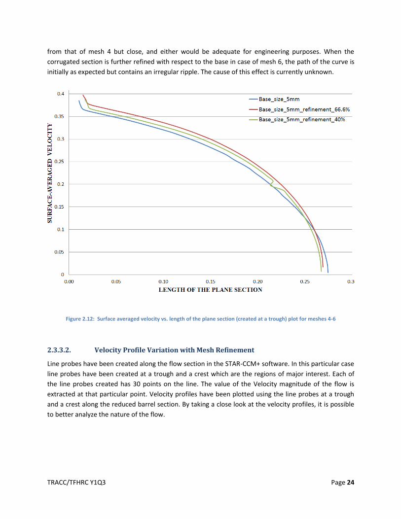
from that of mesh 4 but close, and either would be adequate for engineering purposes. When the
corrugated section is further refined with respect to the base in case of mesh 6, the path of the curve is
initially as expected but contains an irregular ripple. The cause of this effect is currently unknown.
Figure 2.12: Surface averaged velocity vs. length of the plane section (created at a trough) plot for meshes 4-6
2.3.3.2. Velocity Profile Variation with Mesh Refinement
Line probes have been created along the flow section in the STAR-CCM+ software. In this particular case
line probes have been created at a trough and a crest which are the regions of major interest. Each of
the line probes created has 30 points on the line. The value of the Velocity magnitude of the flow is
extracted at that particular point. Velocity profiles have been plotted using the line probes at a trough
and a crest along the reduced barrel section. By taking a close look at the velocity profiles, it is possible
to better analyze the nature of the flow.
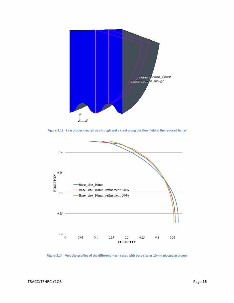
TRACC/TFHRC Y1Q3 Page 25
Figure 2.13: Line probes created at a trough and a crest along the flow field in the reduced barrel
Figure 2.14: Velocity profiles of the different mesh cases with base size as 10mm plotted at a crest
TRACC/TFHRC Y1Q3 Page 26
In Figure 2.14, the x-axis of the plot represents velocity and the y-axis represents the position of the line
probe at a trough in the vertical direction. The minimum unit on the y-axis is 0.2 m and the maximum
unit is 0.4572 m. The y coordinate of the boundary representing the water surface (namely the top of
the reduced culvert section in the CFD study) is at 0.2286 m and the y coordinate of the boundary
representing the bottom of the culvert at the wall in 0.4572 m. The same CAD model has been used for
all the CFD simulations with the co-ordinates of the reduced symmetric barrel section considered from a
trough to a trough as mentioned above. The top surface of the culvert is simulated as a symmetry plane
as mentioned previously which represents an imaginary plane of symmetry in the simulation. It
implicates an infinitely spread region modeled as if in its entirety. The bottom of the culvert is simulated
as a wall with a no slip condition. When velocity is plotted against position, the velocity at the wall is
zero, the first point plotted is the velocity in the cell next to the wall and increases with distance from
the wall. In Figure 2.14, the velocity profiles change as the base size of the mesh is varied. All of these
cases show some mesh dependence but may be adequate for engineering analysis of fish passage.
However, because cases using the relatively small geometry of a barrel section with periodic boundary
conditions complete in a short time further mesh refinement was investigated.
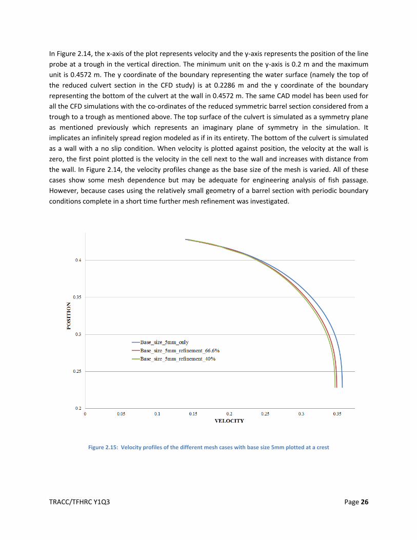
Figure 2.15: Velocity profiles of the different mesh cases with base size 5mm plotted at a crest

TRACC/TFHRC Y1Q3 Page 27
In Figure 2.15 the velocity and the position corresponding to the line probe (at a crest) are represented
on the x and y axis of the plot. With a mesh base size of 5mm, the velocity profiles are very regular. For
the mesh case where the base size is 5mm and no refinement in the corrugated section, the maximum
velocity is a little higher than cases with further refinement in the corrugations. For mesh cases 5 and 6
where the mesh is further refined along the corrugated section in the order of 80% and 66% respectively
there is not much difference in the nature of the velocity profiles although there is large difference in
the number of computational cells. Mesh case 5 consists of 249,174 cells and mesh case 6 consists of
887,369 cells. Mesh 5 is reasonably mesh independent upon further refinement and consumes a
reasonably small amount of computational resources.
Figure 2.16: Velocity profiles of the different mesh cases with base size 10mm plotted at a trough
In Figure 2.16 the velocity profiles of the various mesh cases with base size 10 mm are plotted at a
trough using line probes. The x-axis has a negative scale due to reverse flow in the recirculation zones in
a trough. One of the benefits of flow simulation is that it provides detailed information about
recirculation. Recirculation regions in the flow field are of particular interest since their presence can
have a significant impact on the nature of the flow. As seen in Figure 2.16, there is a difference in the
velocity profiles for the various mesh cases. The mesh case 4 has not been able to capture the effect of
flow recirculation, but as the mesh is further refined along the corrugated section the recirculation of
the flow can be resolved.

TRACC/TFHRC Y1Q3 Page 28
Figure 2.17: Velocity profiles of the different mesh cases with base size 5 mm plotted using at a trough
In Figure 2.17, velocity profiles for the different mesh cases with base size 5 mm at a trough are plotted.
The 5 mm base size with a 66.6% refinement in the trough appears to be the coarsest mesh that is mesh
independent.

TRACC/TFHRC Y1Q3 Page 29
Mesh 1 Mesh 2 Mesh 3
Mesh 4 Mesh 5 Mesh 6
Figure 2.18: Velocity plots of the various mesh cases in the mesh refinement study
The above Figure 2.18 contains the velocity distribution scenes of all the various mesh cases used for the
mesh refinement study plotted at a crest.
Mesh Refinement Conclusions: The mesh refinement studies have been conducted for various base
sizes of the mesh for the symmetric reduced barrel section (considered from a trough to a trough) to
choose the optimum base size of the mesh and also the refinement that needs to be done in the
corrugated section. By analyzing the variation of the surface averaged velocity with respect to the length
of the plane section at a trough and the velocity profiles plotted using line probes at a trough and a crest
the optimum mesh can be selected. With all the CFD analysis done on a 36 inch diameter of the culvert
with corrugation size 3 inches by 1, for a flow depth of 9 inches and a flow velocity of 0.71 feet/second
for zero bed elevation of the culvert, in terms of mesh refinement studies, mesh 5 with a 5 mm base size
and 67% refinement in the corrugation region, which yields a mesh with about 250,000 cells gives mesh
independent simulation results with adequately fast run times.

TRACC/TFHRC Y1Q3 Page 30
2.3.4. Three Dimensional Model of Culvert Flume with Comparison to Experimental Results
The preliminary objective of this study was to develop a computational fluid dynamics (CFD) model to
characterize the three-dimentional (3-D) two-phase (air and water) laboratory model associated with
three different water depths, two different velocities and three bed elevations. The suitability of the CFD
model for fish passage engineering analysis is assessed by comparison with experimental data obtained
from TFHRC. In phase 1 of the study, a three-dimentional multi-phase CAD model, as shown in Figure
2.19, was created in Pro-ENGINEER. The CAD model consists of three parts along the flow direction (z
axis): the intake, the barrel and the diffuser. Since the two-phase VOF model (water and air) is used for
numerical simulation, initially an air layer was included on top of the water domain in the vertical
direction (x axis). The culvert model considered in phase 1 of study is the symmetrical half of the culvert
pipe having annular corrugations without bed elevation as shown in Figure 2.19.
Figure 2.19: Three-dimensional CAD model for multi-phase simulations
The experiments in this study were conducted at the FHWA J.Sterling Jones Hydraulics Laboratory,
located at the TFHRC. The experiments were conducted in a circulating flume. Figure 2.20 provides the
details of the experimental flume dimensions in front and overlook views. The corrugations used are 3
inch by 1 inch annular. Three typical cross sections were monitored in the tests, which were located at
the inlet of the barrel (section 1), the middle of the barrel (section 2) and the end of the barrel (section
3), respectively.
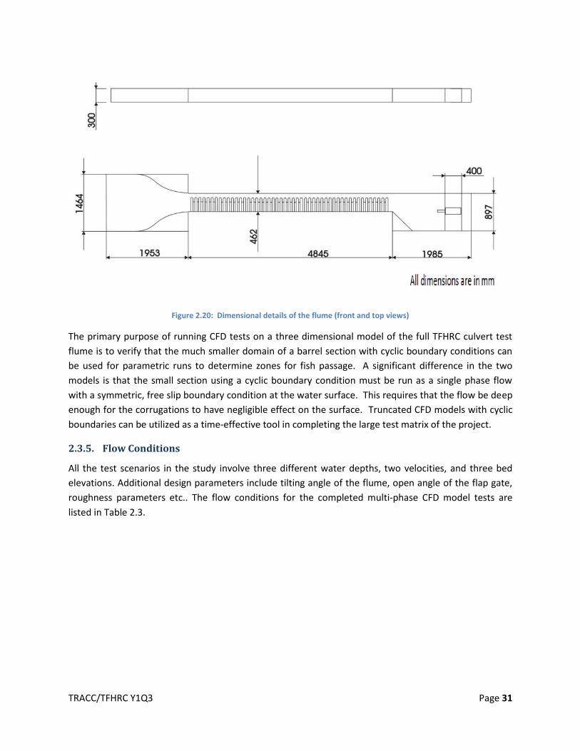
TRACC/TFHRC Y1Q3 Page 31
Figure 2.20: Dimensional details of the flume (front and top views)
The primary purpose of running CFD tests on a three dimensional model of the full TFHRC culvert test
flume is to verify that the much smaller domain of a barrel section with cyclic boundary conditions can
be used for parametric runs to determine zones for fish passage. A significant difference in the two
models is that the small section using a cyclic boundary condition must be run as a single phase flow
with a symmetric, free slip boundary condition at the water surface. This requires that the flow be deep
enough for the corrugations to have negligible effect on the surface. Truncated CFD models with cyclic
boundaries can be utilized as a time-effective tool in completing the large test matrix of the project.
2.3.5. Flow Conditions
All the test scenarios in the study involve three different water depths, two velocities, and three bed
elevations. Additional design parameters include tilting angle of the flume, open angle of the flap gate,
roughness parameters etc.. The flow conditions for the completed multi-phase CFD model tests are
listed in Table 2.3.

TRACC/TFHRC Y1Q3 Page 32
Table 2.3: Flow conditions
Water Depth 3 inch 6 inch 9 inch
Bed elevation 0 0 0
Air depth(inch) 2.5 3 2.5
Mean velocity (m/s) 0.2164 0.2164 0.2164
Tilting angle of the flume
(degree) 1 0.125 0.07
Tilting angle of the flap gate
with respect to the horizontal
(degree)
12.5 18 28
2.3.6. Results Using VOF Multiphase Model
Velocity distributions are plotted over a plane cut through a culvert barrel trough that is located in the
middle of the culvert. For each water depth, the velocity distribution across the whole multi-phase
cross-section is given on the left, and the plot on the right covers only the lower zone containing water.
Also, the 0.5 VOF curves are plotted on top of the velocity contours, which indicate the corresponding
water surface. The results for 3 inch, 6 inch, and 9 inch water depth are illustrated in Figure 2.21, Figure
2.22, and Figure 2.23 respectively.
Figure 2.21: Velocity distribution across trough section of the multi-phase model for 3 inch water depth

TRACC/TFHRC Y1Q3 Page 33
Figure 2.22: Velocity distribution across trough section of the multi-phase model for 6 inch water depth
Figure 2.23: Velocity distribution across trough section of the multi-phase model for 9 inch water depth
2.3.7. Comparison with the Single Phase Model
In the multi-phase CFD model for the full-scale flume, if the longitudinal VOF changes indicate that the
water level is nearly flat along the culvert, it is possible to set up a single phase model to simulate the
flow. Figure 2.24 illustrates the comparison of the velocity distribution between the multi-phase model
and full scale single phase model for 6 inch water depth. Note that the maximum velocity occurred in
the single phase case is 0.42 m/s, which is larger than 0.38m/s in the multi-phase case.

TRACC/TFHRC Y1Q3 Page 34
Figure 2.24: Multi-phase model vs. full flume single phase model illustrating velocity distribution across trough section for 6 inch water depth
2.3.8. Comparison with Laboratory Data
Particle Image Velocimetry (PIV) and Acoustic Doppler Velocimetry (ADV) are two methods used to
capture the velocity data from laboratory experiments. Acoustic Doppler Velocimeters are capable of
reporting accurate values of water velocity in three directions even in low flow conditions. The main
objective of the PIV tests is to obtain a 3-dimensional high-resolution velocity distribution, which is
convenient for visual comparisons with CFD results.
Comparisions of the CFD data with laboratory data for 6 inch and 9 inch water depths have been done.
The agreement levels between multi-phase model results and experimental results for 6 inch water
depth are depicted in Figure 2.25 and Figure 2.26. Since neither the PIV nor ADV can capture the data
for the whole section, the corresponding data ranges are framed out in CFD results respectively.

TRACC/TFHRC Y1Q3 Page 35
Figure 2.25: CFD velocity contour plot with ADV cut area (upper) vs. ADV velocity contour plot (lower) for 6 inch water depth on the trough section

TRACC/TFHRC Y1Q3 Page 36
Figure 2.26: CFD velocity contour plot with PIV cut area (upper) vs. PIV velocity contour plot (lower) for 6 inch water depth on the trough section
The comparison between multi-phase CFD model results and ADV results for 9 inch water depth are
shown in Figure 2.27, in which the comparable areas are much larger than those for 6 inch. The
comparison of multi-phase CFD results and PIV results for 9 inch is still proceeding.

TRACC/TFHRC Y1Q3 Page 37
Figure 2.27: CFD velocity contour plot with ADV cut area (upper) vs. ADV velocity contour plot (lower) for 9 inch water depth on the trough section
The preliminary simulation results (for 0 bed elevation) reveal that the three-dimentional (3-D) two-
phase (air and water) CFD models solved in STAR-CCM+ yield reasonably good agreement in the velocity
distributions, compared with both the PIV and ADV data. The velocity distribution contours obtained
from the CFD simulation are much closer to the PIV observation results. Furthermore, the PIV data
capture range is larger than that of ADV because ADV can hardly get the data near the water surface and
adjacent to the culvert boundary.
Note that the full flume single phase CFD model has better concurrence of velocity distribution with
experimental measurements. Based on the discussion in Section 8.1.3.7, the single phase velocity

TRACC/TFHRC Y1Q3 Page 38
magnitude is larger than that of the multi-phase CFD model. Taking 90% of the magnitude of velocity
obtained from the single phase CFD model, the visual agreement with the PIV results is presented in
Figure 2.28.
Figure 2.28: 90% single phase CFD velocity contour plot with PIV cut area from (upper) vs. PIV velocity contour plot (lower) for 6 inch water depth on the trough section

TRACC/TFHRC Y1Q3 Page 39
Conclusions for Comparison with Experiment: The experimental work is not yet complete, and
therefore this assessment is preliminary. The experimental PIV and ADV data show differences that are
of the same order as the differences between either of the experimental approaches and the CFD
results. All of these show significant variation of velocity over culvert cross sections with higher velocity
near the center. Making engineering use of data obtained from CFD analysis on cross section variation
of velocity will likely be an improvement over just using the mean velocity in design of culverts for fish
passage. While there are differences in both of the experimental techniques and the multiphase and
single phase CFD approaches to obtaining the cross section velocity distribution, the information is much
closer to reality than an assumed uniform mean velocity. Culvert design for fish passage cannot come
close to conditions that would exhaust fish attempting to swim through the culvert, and therefore the
use of data that has some uncertainty but is much better than current practice can still yield a major
improvement in design practice.
2.3.9. References
1. Matt Blank, Joel Cahoon, Tom McMahon, “Advanced studies of fish passage through
culverts: 1-D and 3-D hydraulic modeling of velocity, fish expenditure and a new barrier
assesment method,” Department of Civil Engineering and Ecology, Montana State
University, October, 2008 .
2. Marian Muste, Hao-Che Ho, Daniel Mehl,“Insights into the origin & characteristic of the
sedimentation process at multi barrel culverts in Iowa”, Final Report, IHRB, TR-596, June,
2010.
3. Liaqat A. Khan, Elizabeth W.Roy, and Mizan Rashid, “CFD modelling of Forebay
hydrodyamics created by a floating juvenile fish collection facility at the upper bank river
dam”, Washington, 2008.
4. Angela Gardner, “Fish Passage Through Road Culverts” MS Thesis, North Carolina State
University, 2006.
5. Vishnu Vardhan Reddy Pati, “CFD modeling and analysis of flow through culverts”, MS
Thesis, Northern Illinois University, 2010.
6. Kornel Kerenyi, “Final Draft, Fish Passage in Large Culverts with Low Flow Proposed Tests”
unpublished TFHRC experimental and CFD analysis of culvert flow for fish passage work
plan, 2011.

TRACC/TFHRC Y1Q3 Page 40
3. Computational Multiphysics Mechanics Applications
3.1. Multiphysics Simulation of Salt Spray Transport
The Turner Fairbank Highway Research Center (TFHRC) currently is interested in studying the transport
of salt spray generated by vehicle tires from the pavement up to the exposed steel support beams of
steel bridges as the tires roll over wet pavement. The research is aimed to update the Technical
Advisory, which is already over 20 years old, with results based on current state-of–the-art
computational analysis and experimental data acquired at critical locations.
3.1.1. Estimate for Water Content in Semi-Trailer Truck’s Wake
In [1], the modeling of the transport of salt-water mixture from the pavement surface to the underside
of steel bridges was shown to involve three phases. The first phase is the lifting of the salt-water mixture
from the road surface by the tires and ejecting the mixture into the swirling air around the wheels. The
second phase is the egression of the mixture from the wheel region to the outside of the vehicle and
from the under carriage of the vehicle, with eventual egression from the rear of the vehicle. Here the
mixture will be referred to as a cloud, which is the vortex wake of the vehicle driving over a wet roadway
(Figure 3.1). The third phase is the impact of a second vehicle—which is following the first vehicle—into
the cloud and the potential transport of a portion of the cloud onto the steel beams.
Figure 3.1: Egression of the salt-water air mixture into the air outside of the vehicle forming two side-of-vehicle clouds and a rear undercarriage cloud [1]
Up to now, most of the work done at the Transportation Research and Analysis Computing Center
(TRACC) was to develop tractable models and modeling techniques for the MM-ALE approach. During
this time, the entire air domain was assumed to be just air without any water content. This study
estimates the water content of the resulting cloud formed during the second phase based on
computational fluid dynamics (CFD) simulation results presented in [3] and presents recommended
values for densities to be used for the cloud material in future simulations.

TRACC/TFHRC Y1Q3 Page 41
3.1.1.1. Approach
To date, an initial search of the literature did not turn up any experimental results for the water content
in the vehicle wake, and this is unfortunate because experimental test data adds credibility to simulation
results. However, a paper [3] based on numerical simulations using the STAR-CD software contains
results that could be used in our LS-DYNA MM-ALE simulations.
In [3], spray dispersion simulations using a simplified semi-trailer model—the Generic Conventional
Model (GCM)—were performed. Two cases were considered: without trailer-mounted base flaps and
with trailer-mounted base flaps. Because the droplet sizes could range from 0.01 mm to 1 mm
(0.0003937 inch to 0.03937 inch) this would entail an extremely large number of droplets on which to
perform calculations, so a “parcel” approach was adopted. In the parcel approach, each parcel/particle
represents a collection of droplets with a fixed mass. For our MM-ALE approach, this is ideal because we
are not modeling droplets but are modeling the movement of multiple materials (air, cloud, and vehicle)
through a fixed computational mesh. So we are interested in the mass properties of each of these
materials in order to compute their movement under, around and over the bridge as the truck travels
under the bridge and displaces the air and cloud.
3.1.1.2. Results
In [3], two designs were considered for the trailer: without trailer-mounted base flaps and with trailer-
mounted base flaps. The flaps were shown to have an effect on the distribution of the parcels in the
trailing wake (cloud). Figure 5, p. 12 in [3] shows the parcel distribution obtained for the case without
flaps and with flaps, respectively.
A close study of those graphics shows that for the case with flaps the parcels tend to be lower and rise to approximately one-third to one-half the height of the trailer. In contrast for the case without flaps, the particles rise to the top and possibly above the top of the trailer. The importance of this observation is that a trailing vehicle (car or truck) then has the potential to push these parcels up higher—perhaps between the bridge’s beams. Another observation is that the mean diameter of most of the parcels appears to be 0.54 mm (0.02126 inches) or less. In [3] a 13 meter long by 5 meter wide by 3.3 meter high (42.6 ft. by 16.4 ft. by 10.83 ft.) sampling domain was used, and the number of parcels in the domain was computed for the two cases. Note, one parcel contains 22.2 grams of water (0.0485 lb.). A conversion from parcels to mass was performed for the two cases, and the results are shown in Table 3.1.
Table 3.1: Water content in sampling domain generated by a GCM traveling at 29 m/s (65 mph) [1]
Without Trailer-Mounted Flaps With Trailer-Mounted Flaps
2.15 parcels/m3 0.0609 parcels/ft3 3.4 parcels/m3 0.0963 parcels/ft3
48.375 g/m3 0.00295 lb/ft3 76.5 g/m3 0.00467 lb/ft3

TRACC/TFHRC Y1Q3 Page 42
The density of water is 1,000 kg/m3, and for the case without flaps the mass per cubic meter is 48.375 g;
so the volume of the water is 48.375 * 10-6 m3. For the case with flaps case, the volume of water is
76.5 * 10-6 m3.
For an initial analysis, it is assumed that the parcel distribution is uniform throughout the sampling
domain. The density of air at sea level and 15 degrees Celsius is 1225.21 g/m3. So for the case without–
flaps, the combined mass of the air and water in a cubic meter is 1273.59 grams, and for the case with-
flaps, it is 1301.71 grams. Table 3.2 shows the resulting densities that should be used for the cloud
material in the MM-ALE simulations. The ratio of the density of the cloud to the density of air, which is
seen to be from 4% to 6% larger than that of the air alone, appears to be reasonable.
Table 3.2: Cloud material densities generated by a GCM traveling at 29 m/s (65 mph)
Trailer-Mounted-Flaps Without With
Mass of air plus water (g) 1273.59 1301.71
Density (g/m3 ) 1273.59 1301.71
Density ratio 1.039 1.062
Looking at Error! Reference source not found., the parcels are concentrated near the lower third
(approximately) of the sampling domain. So for this case, the density would be higher. By considering all
the parcels to be located in the lower third of the sampling box, the density of the cloud, becomes 19 %
greater than air.
3.1.1.3. Discussion and Recommendations
Based on prior simulations reported in Reference [3], an estimate of the water content in the cloud (i.e.,
the trailing vortex wake) of a semi-trailer truck was made. Reference [3] used a sampling box to collect
data on the distribution of parcels (i.e. a collection of water droplets) behind the semi-trailer for the
case where the trailer had flaps and the case without flaps. Our initial estimate for TRACC’s calculations
assumed a uniform distribution within the sampling box and showed that the density of the cloud was
between 4-6% higher than air. Thus, adjusting the density of the material representing the cloud by
these values would give a fair engineering representation for the cloud behavior in the MM-ALE
simulations. Using the uniform distribution assumption with a 4-6% increase in cloud density is a
reasonable perturbation that should not generate any numerical surprises in the simulation runs.
Examining the figure showing parcel distribution within the bounding box for the case with flaps shows
that most of the parcels appear to be in the bottom third of the box. Thus, when the assumption of
uniform distribution is relaxed, and a higher distribution near the lower third of the box is made, the
density would be 19% higher than the density of air. A close study of the graphics shows that for the
case with flaps the parcels tend to be lower and rise to approximately one-third to one-half the height of
the trailer. In contrast for the case without flaps, the particles rise to the top and possibly above the top
of the trailer. The importance of this observation is that a trailing vehicle (car or truck) then has the

TRACC/TFHRC Y1Q3 Page 43
potential to push these parcels up higher—perhaps between the bridge’s beams. Another observation is
that the mean diameter of most of the parcels appears to be 0.54 mm (0.02126 inches) or less.
Another issue that needs to be addressed is the appropriate equation of state for the cloud material. For
simulations performed to date, a polynomial equation for air was used because only the air was
modeled. When moisture is considered along with the air at a density of 4-6 % greater than air,
engineering judgment is to use the equation of state for air for the cloud but to use the higher densities.
For a cloud density of 19% greater than air, additional thought needs to be given on the appropriate
equation of state, and this will be presented in a future work.
During this past winter season, TRACC CSM staff made personal observations of the trailing wake (cloud)
of semi-trailers on I88 while traveling at 105 kmph (65 mph). The qualitative observation was that the
bulk of the salt spray reached about 2.5 meters (8 feet) high—a little over the top of the car.
Subsequently, during this spring’s rainy season, similar observations were made on a local highway
while traveling at 80 kmph (50 mph), and it appeared that the spray reached the top of the trailer (4.1
m/13.5 ft.). It is apparent that the cloud configuration will depend on the semi-trailer truck and the
specific shape of the tractor, trailer, undercarriage features, etc.
It is recommended that field data be obtained for the water distribution in a cloud to complement
numerical simulations. Perhaps, movies could be taken alongside and behind a semi-trailer to
qualitatively get an idea of the size of the cloud. This could be done in the winter time when road salt is
present. In addition during the summer/fall, water could be spread over a short stretch of highway—say
two to three trailer lengths long—and video cameras could be positioned along the roadway to record
the cloud behavior as a semi-tractor trailer traveled over the wet pavement. To enhance cloud visibility,
the water could be colored or black screens could be positioned on the side of the roadway opposite to
the video recorders. This experiment could be done on the open road and under a bridge.
The beginning of a quantitative assessment could be made by developing a device that could be
mounted on the front of a small truck and would collect water at different Y-Z locations (Y is in the
direction transverse to the truck, and Z is in the vertical direction) behind a semi-trailer truck for a length
of time equal to a distance of 13 m, which is the length of the sampling domain used in [3]. This data
could be compared to the simulation results reported in [3] and also would be of value, in and of itself.
3.1.1.4. References
1. Kulak, R. F., Application of Multiphysics Mechanics to Modeling Salt Spray Transport onto Steel Support Beams of Bridges, RFK Engineering Mechanics Consultants, Technical Note: TRACC-TFHRC-001, November 13, 2010.
2. Kulak, R. F., Feasibility Study on using MM-ALE Approach to Modeling Salt Spray Transport onto Steel Support Beams of Bridges, RFK Engineering Mechanics Consultants, Technical Note: TRACC-TFHRC-002, December 02, 2010.
3. Paschkewitz, J. S., Simulation of Spray Dispersion in a Simplified Heavy Vehicle Wake, Lawrence Livermore National Laboratory, UCRL-TR-218207, January 17, 2006.

TRACC/TFHRC Y1Q3 Page 44
3.1.2. Simulation of a Semi-trailer Truck Passing Through a Bridge Underpass
Based on the recent study, a finite element model of the Raleigh - Tamarack Overpass (Bridge No. 4172) was updated. The domain of the air over the truck was significantly extended to minimize the effect of the boundaries on the flow of the air around the vehicle and the bridge beams. The model is shown in Figure 3.2. The main area of interest is built of hexahedral elements with edge size of 100 mm (darker blue area in the drawing). The rest of the domain is built of elements that increase in size further out from the vehicle. The basic statistics of the model are listed in Table 3.3.
Figure 3.2: Setup for analysis of the air movement under the bridge
Table 3.3 Statistics of the FE model of the bridge
Entity Count
Number of Nodes 4,622,267
Number of Shell Elements 829,082
Number of Solid Elements 3,774,363
Number of Deformable Solids 3,301,688
Total number of elements 4,603,445
The simulation was performed for 3.0 seconds of real time, which took about 72 compute-hours to
complete. Several quantities were tracked in the simulations for visualization of the results. The most
important quantities were the spatial trajectories of tracer particles in the air. They represent virtual,
massless particles that follow precisely the flow of the air. A three-dimensional matrix of tracer particles
was defined in the volume before and under the overpass. The particles were defined in horizontal
planes at four vertical levels:

TRACC/TFHRC Y1Q3 Page 45
the wheel level,
the engine level
the windshield level
the top surface of the trailer level
Nine cross sections in the travel direction were defined, and at each vertical level in each cross section,
five tracer particles were defined in the direction perpendicular to the travel direction. This provided the
ability to study the motion of the air as the truck moves through the underpass. Overall there were 180
tracer particles defined.
For each level, the figures below show the particle trajectories at different times in the simulation. In
addition, velocity isosurfaces are shown on each of the figures to provide a look at the motion of the air
as the truck passes through the underpass. Figure 3.3 shows trajectories of the particles at the level of
the wheel axles. Most of the particles stay at this level except for the ones being trapped behind the
cabin. These trapped particles can be lifted up and dragged by the vehicles for long distances.
In Figure 3.4, the trajectories of the particles at the engine hood level are shown. The particles that are
along the mid-width of the vehicle are lifted up from the hood level to the trailer-top level and are
dragged along with the vehicle. The particles away from the mid-width of the vehicle are pushed to the
sides of it and are not lifted higher.
In Figure 3.5, the trajectories of the particles located at the windshield level are shown. These particles
are also smoothly pushed up to the top surface of the trailer. Once the particles get to the back of the
trailer, they become part of the developing vortex wake. This causes the particles to move down rapidly
and follow the back of the trailer – i.e., the particles are entrapped in the trailer’s vortex wake.
Eventually, some of the particles exit from the wake and appear to move into the space between the
bridge beams. The particles at the trailer’s top-surface-level behave in a similar way (see Figure 3.6);
they also appear to find their way into the space between the bridge beams.
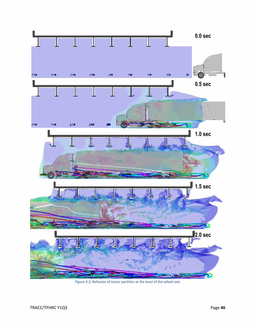
TRACC/TFHRC Y1Q3 Page 46
Figure 3.3: Behavior of tracer particles at the level of the wheel axis
0.0 sec
0.5 sec
1.0 sec
1.5 sec
2.0 sec

TRACC/TFHRC Y1Q3 Page 47
Figure 3.4: Behavior of tracer particles at the level of the engine hood
0.0 sec
0.5 sec
1.0 sec
1.5 sec
2.0 sec
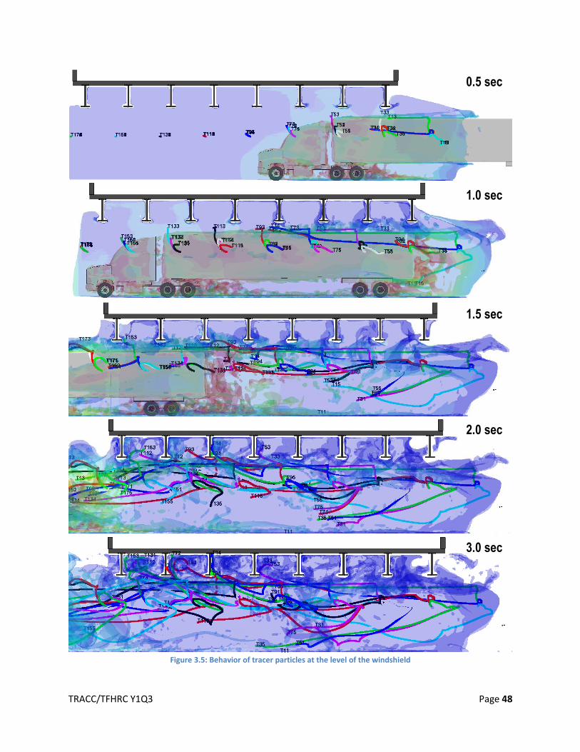
TRACC/TFHRC Y1Q3 Page 48
Figure 3.5: Behavior of tracer particles at the level of the windshield
0.5 sec
1.0 sec
1.5 sec
2.0 sec
3.0 sec

TRACC/TFHRC Y1Q3 Page 49
Figure 3.6: Behavior of tracer particles at the level of the top surface of the trailer
0.5 sec
1.0 sec
1.5 sec
2.0 sec
3.0 sec

TRACC/TFHRC Y1Q3 Page 50
Next, the air motion between the beams as the truck passes under the bridge is studied. Velocity vector plots with superimposed velocity isosurfaces are presented to understand the motion. A typical plot is shown in Figure 3.7 where the small arrows show the velocity at a specific instant of time. Because these vectors are difficult to see, a large red arrow is superimposed on the plots to show the general movement of the air in a given region. Figure 3.8 shows the middle cross section – i.e., the area perpendicular to the direction of truck motion -- through the air domain and velocity vectors together with the velocity isosurfaces. At 0.5 sec, the vehicle is approaching this cross section, and the air is starting to move up. At 1.0 sec, when the vehicle is passing under this cross section, the air on the top part of the domain behaves in a similar way. Increased velocities can be seen in the proximity of the vehicle wheels and around the trailer. At 1.5 sec, the vehicle is past this cross section, and the velocity vectors have changed directions. Now they are pointing downward, and as mentioned previously, the air is sucked down to the vacuum created behind the truck. With time, the vectors continuously change their directions. It is important to note that this mechanism could potentially cause transport of the air containing the water-salt spray from the road surface to the bridge beams.
Figure 3.7: Close up view of the velocity vectors

TRACC/TFHRC Y1Q3 Page 51
Figure 3.8: Velocity vectors in the middle cross section of the air domain
0.5 sec 1.0 sec
1.5 sec 2.0 sec
3.0 sec

TRACC/TFHRC Y1Q3 Page 52
The present work is a first look at the behavior of the air under a bridge as a semi-trailer truck passes through the underpass: therefore, it must be considered very preliminary. It was assumed that the air was stationary and the truck was moving at 60 mph. Stable calculations were performed up to 3 seconds of simulation time, which allowed the truck to enter and completely pass under the bridge.
In looking over the results, it is beneficial to divide the simulation into two phases. The first phase looks at the air motion as the air approaches and passes around the semi-trailer truck; the second phase considers the air motion after the truck has passed – i.e., the motion of the air behind the truck. During the first phase, it was seen that the air moves over, under and around the sides of the truck. Simulations showed that the air particles originally at the level of the top of the trailer – i.e., the highest level that was traced to date – appear to move to the flange area around the bottom of the beams. They do not appear to reach the web of the beams or the bottom of the bridge deck. Perhaps, particles originally at the level of the flanges could be pushed higher into the space between the beams.
Examining the air motion during the second phase reveals some interesting behavior. During this phase, complex wake vortices develop behind the vehicle from the four edges of the trailer. To a first order, the simulations appear to capture this motion; however, at this time there is uncertainty associated with the accuracy. Keeping this in mind, results show that the air originally at the mid-height of the windshield or higher can be transported into the spaces between the bridge beams.
The results from computational fluid dynamics simulations performed by Lawrence Livermore National Laboratory (see Section 3.1.1) showed that the road surface water can be propelled up to at least to the height of the top of a semi-trailer by the trailer’s vortex wake. In view of this, a second semi-trailer truck would now be passing through the first trailer’s vortex wake that potentially contains a mixture of air and salt water at levels near the top of the trailer, which could then be propelled between the beams.
In the next quarter, it is planned to continue studies using the current model. The following cases will be considered:
- A truck traveling through an air domain without a bridge; - A truck traveling through an underpass with a vertical embankment close to the traffic lane; - A truck traveling through an underpass with a vertical embankment close to the traffic lane and
larger distance between the trailer top and bottom of the bridge beams; - Additional runs of the above cases using two trucks – a leading truck and a trailing truck.
Finally, the details of the trailing vortex wake will be studied.
3.2. Wind Engineering
The work presented in this section was performed by graduate students at Northern Illinois University
under the partial guidance of the CSM staff.

TRACC/TFHRC Y1Q3 Page 53
3.2.1. Vehicle Stability under High Wind Loadings
3.2.1.1. Literature Review
The previous quarterly report presented the dynamic equation of motions for a truck with forward
velocity and external loading (wind force). As the formulation of equations was complex due to
incorporation of various body parts of the truck, there was a necessity for simplification of the previous
model.
In order to get a clear understanding of the dynamic behavior of a truck, a model with three rigid bodies
as sprung mass, front axial and rear axial (Figure 3.9) was used [1]. The equations of the model were
simpler compared with the previous version as it excludes the compliance of other parts. The equations
of the truck with three rigid bodies are given as follows [1]:
( ) (3.1)
(3.2)
( ) ( ) ( )
( ) ( )
(3.3)
( )
( ) ( )
( ) ( )
(3.4)
( )
( ) ( )
( ) ( )
(3.5)
Where,
= height of roll axis, measured upwards from ground

TRACC/TFHRC Y1Q3 Page 54
= active roll torque
= suspension roll damping rate.
k =suspension roll stiffness
kb = vehicle frame torsional stiffness
kt = tire roll stiffness
= vehicle coupling roll stiffness
= vehicle coupling yaw stiffness
= absolute roll angle of sprung mass.
= absolute roll angle of unsprung mass
= roll moment of inertia of sprung mass, measured about origin of coordinate system
= yaw-roll product of inertia of sprung mass, measured about origin of coordinate system
= yaw moment of inertia of total mass, measured about origin of coordinate system
=
= partial derivative of net tire yaw moment with respect to sideslip angle.
=
= partial derivative of net tire yaw moment with respect to yaw rate.
=
= partial derivative of net tire yaw moment with respect to steer angle.
ms= Sprung mass,
h = height of center of sprung mass, measured upwards from roll center
m = total mass
U = forward speed
= yaw rate
=
partial derivative of net tire lateral force with respect to sideslip angle
= sideslip angle
=
= partial derivative of net tire lateral force with respect to yaw rate
=
= partial derivative of net tire lateral force with respect to steer angle

TRACC/TFHRC Y1Q3 Page 55
= steer angle
These equations could be effectively solved using the state space method. Mathematical expression of
state space representation model is as follows [1]:
Where,
x = [β ]T
u = [ ]T
E =
0 0 0 0
0 0 0 0
0
( )
0 0 0 0
( )
0 0 0 0
0 0 1 0 0 0
A =
E-1
0 0 0 0
0 0 0 0
0
( ) ( )
( )
0
( ) ( )
( )
0

TRACC/TFHRC Y1Q3 Page 56
0 0 0 1 0 0
B0 = E-1 0 0 1 0 1 0 T
0 0 1 1 0 0
B1 = E-1 [ 0 0 0]T
3.2.1.2. Conversion of wind velocity to wind pressure
The conversion of wind velocity to wind pressure is necessary because the wind is described in terms of
velocity and in the finite element analysis the velocities are attached to the nodes and pressure is
applied to elements. The loading on elements would provide more accurate results compared to the
node loading.
The pressure due to wind velocity can be computed using the following conversion:
Where,
P = Pressure (N/m2)
C = Drag coefficient
D = Density of air (1.25 Kg/m3)
V = Speed of air (m/s)
The drag coefficient is a dimensionless quantity and it depends upon the surface area under the
influence of attacking wind. The drag coefficients for flat and cylindrical body are approximated as
follows:
Drag coefficient for flat surface = 1
Drag coefficient for cylindrical surface = 0.67.
3.2.1.3. Development with the FEM
After understanding the spring-damper system in LS-DYNA, it was necessary to study the motion of a
node on a surface. To perform the analysis, a flat surface was created with two beam element and two
massless nodes attached to it (Figure 3.10). These nodes were given a velocity and constraint so as to
follow the beam element from start to end.

TRACC/TFHRC Y1Q3 Page 57
With the success to the above analysis, a spring element was attached to the nodes and a block was
mounted on it (Figure 3.11). To verify the proper behavior of the spring, an initial displacement was
given and it produced the appropriate result.
After verifying the behavior with the above model, the task was to give an appropriate loading to the
vertical face of block in order to understand the effects of wind pressure (Figure 3.12). Two types of
wind pressure were given to the block, a constant load and a sine load.
The properties of the model are:
Mass = 5.88 Kg,
Stiffness = 60 N/mm,
Length of spring = 50 mm,
Amplitude = 0.01,
Frequency = 100 Hz,
Forcing function = Amplitude*SIN(2*3.14*Frequency*TIME)
Figure 3.13 shows the graph of horizontal displacement of the block with the application of sinusoidal
wave as a forcing function.
Theoretically, the equation of motion of the block with vertical springs and horizontal sine forcing
function (Figure 3.12) is given by:
√ (3.6)
Where,
m = Mass of the block,
k = Stiffness of spring,
l = original length,
x = Displacement from static equilibrium position
F0 = Forcing function (sine wave)
3.2.1.4. Ford F-800 truck development
A Ford F-800 truck model (Figure 3.14) was taken from the National Crash Analysis Center (NCAC)
website [2]. The raw file contained a FEM model of the truck with six rigid walls attached to each tire
and forward velocity. This model was studied and modified according to the requirements of the
TRACC/TFHRC Y1Q3 Page 58
analysis. The basic modifications consist of creating a new rigid wall which was attached with the body
of the truck, changing the forward velocity, and applying damping and pressure load (Figure 3.15).
Damping Estimation:
In order to gain a clear understanding of the behavior of the truck, the truck was made stationary (no
forward velocity). Initially the truck was ideally modeled and to simulate the actual environmental
condition, the truck model was allowed to settle on its suspensions. The displacement graph of the ideal
truck is shown in (Figure 3.16). The graph contains displacement of three nodes from which the third
node shows a clear displacement and it was used for further analysis. The displacement graph gives the
properties of the suspension and the results of applying a global damping value to the system.
The damping estimation for LS-DYNA is calculated as follows:
(3.7)
{3.8)
Where,
T = Time period between two successive crest or troughs of the displacement graph (Figure 3.16).
D = critical damping factor.
The displacement graph gives the value as follows:
T = 0.25 seconds
This reflects,
Various damping values below the critical damping value from 20 to 45 in multiples of 5 were given to
the model. An optimum damping value was chosen in order to stabilize the truck and further application
of wind load was possible without the effect of a global damping factor. Figure 3.17 gives the
displacement obtained from various damping values.
3.2.1.5. Wind Loading
A wind pressure loading was given to the side of the trailer part of the truck. When a pressure was given
with the help of conventional way (load_segment) it was seen that the pressure remains exactly
perpendicular to the surface irrespective of the trailer position. This was contradicting with the actual
situation as the wind loading should be along the ground surface. This actual situation was simulated in
the model by developing a wind load with the help of the load_segment_nonuniform keyword

TRACC/TFHRC Y1Q3 Page 59
command. This requires the creation of a local co-ordinate system and the load directed with the help of
directional cosines.
Figure 3.9: Single unit rigid vehicle [1]
Figure 3.10: Mass-less nodes moving on a beam element

TRACC/TFHRC Y1Q3 Page 60
Figure 3.11: Motion of block attached with spring elements
Figure 3.12: Wind loading applied at the side of the block
Figure 3.13: Displacement graph of block model with vertical springs and horizontal load
-3
-2
-1
0
1
2
3
0 2 4 6 8 10
Y-D
isp
lace
men
t
Time (s)

TRACC/TFHRC Y1Q3 Page 61
Figure 3.14: FEM Model of a Ford F-800 truck obtained from NCAC [2]
Figure 3.15: FEM model modified according to the analysis

TRACC/TFHRC Y1Q3 Page 62
Figure 3.16: Graph of free displacement of truck on the suspension
Figure 3.17: Displacement graph of various damped values
3.2.1.6. References
1) Sampson, D. J. M., “Active Roll Control of Articulated Heavy Vehicles”, A dissertation for the
Degree of Doctor of Philosophy, submitted to the University of Cambridge, September 2000.
2) http://www.ncac.gwu.edu/
-60
-50
-40
-30
-20
-10
0
10
0.0 0.2 0.5 0.8 1.0 1.3 1.5 1.8
Z-D
isp
lace
men
t (m
m)
Time (s)
-30
-25
-20
-15
-10
-5
0
0.00 0.25 0.50 0.75 1.00 1.25 1.50 1.75
Z-D
isp
lace
men
t (m
m)
Time (s)
D20
D25
D30
D35
D40
D45

TRACC/TFHRC Y1Q3 Page 63
3) Chen, F. and Chen, S., “Assessment of vehicle safety behavior under adverse driving
conditions”; 11th American Conference on wind loading, San Juan, Puerto Rico, June 22-26,
2009.
4) Winkler C.B. and Ervin R.D., “Rollover of heavy commercial vehicles”, UMTRI-99-19, The
University of Michigan, Transportation Research Institute, Michigan, August 1999.
3.2.2. Electromagnetic Shock Absorber for Vehicle Stability under High Wind Conditions
New work done during the third quarter involved the analytical modeling of the electromagnetic shock
absorber (EMSA) as well as its incorporation into the ¼ car Simulink model. The Simulink model utilizes
an actual road profile as the disturbance for the system and the data is automatically exported into
Microsoft Excel for post-processing. Also, FEM simulations of the Ford F800 truck model were
performed to obtain mass, stiffness and damping properties.
3.2.2.1. New EMSA Model
The new analytical model of the EMSA is based upon [1]. The operation of this EMSA is very similar to
the original proposed model. The main difference is that this new model utilizes two permanent magnet
(PM) assemblies surrounded by a moving coil assembly mounted to a sliding armature [1]. When the coil
assembly moves in and out of the PM assemblies, a voltage is produced in the coils.
In order to provide control over the EMSA, a voltage input is calculated based upon the relative velocity
seen by the EMSA and the desired force. The desired force is calculated based upon the four states of
the ¼ car model, [see Equation (8.14) from the previous TRACC Quarterly Report (Y5Q2)]. The actual
force of the EMSA does not exactly match the desired force, since the EMSA force is limited by the
direction of the generated voltage. In other words, the input voltage must be in the same direction as
the generated voltage.
The induced or generated voltage in each coil section is:
(3.9)
Where is the radius of the coil assembly, is the number of turns per length, is the height or length
for the section, is the relative velocity seen by the EMSA and is the magnetic flux from the PM
assembly. It is evident that the total length of wire for each coil section is:
(3.10)
The force generated opposing the motion of the coil form is:
(3.11)
The circulating current in the coil assembly is denoted by . The total voltage for each section of the coil
assemblies is the summation of the generated voltage and the input voltage:
(3.12)

TRACC/TFHRC Y1Q3 Page 64
The input voltage is determined by using ohms law, by substituting the total voltage divided by the
resistance into Equation (3.11). After solving for the voltage input, the final equation takes the form:
[
] [ ] (3.13)
The Simulink model that calculates the input voltage has conditional blocks that ensure the input
voltage is in the same direction as the circulating voltage. If the input voltage is in the opposite direction
of the circulating voltage, the conditional blocks set the input voltage to zero. The EMSA force for a
given road profile is very similar to the desired force. Shown in Figure 3.18 is the desired force, which is
based upon the states of the system. Shown in Figure 3.19 is the EMSA force, which is based upon the
desired force, the relative velocity and the conditional blocks. The major difference between the two
plots is that the EMSA force tends to dwell near zero due to the conditional statements. The gain values
for the desired force were obtained from [2].
Figure 3.18: Plot of the Desired Force, based upon the states
-100
-75
-50
-25
0
25
50
75
0 10 20 30 40
Force (N)
Time (sec)

TRACC/TFHRC Y1Q3 Page 65
Figure 3.19: Plot of the EMSA force
3.2.2.2. Improved Simulink Model
The Simulink model now incorporates an actual road profile obtained from the Long Term Pavement
Performance (LTPP) Department under the U.S. Department of Transportation Federal Highway
Administration. The road profile is an array of data points, which are vertical deflection measurements.
The measurements are separated by a distance of four feet. Shown in Figure 3.20 is a representation of
the road profile data. However, the Simulink model needs the road profile data to be in terms of time.
This is achieved by assuming the vehicle is traveling at a constant velocity. Shown in Figure 3.21 is the
actual road profile plot used in the Matlab-Simulink model.
Figure 3.20: Schematic of the road profile data
-100
-75
-50
-25
0
25
50
75
0 10 20 30 40
Force (N)
Time (sec)

TRACC/TFHRC Y1Q3 Page 66
Figure 3.21: Actual road profile plot
Other improvements to the Simulink model include: the incorporation of the EMSA model to the ¼ car
model and data exportation to Microsoft Excel for post-processing. The Excel file plots the four states of
the system, as well as the sprung mass acceleration. RMS values for the sprung mass acceleration,
suspension deflection and tire deflection are calculated. Shown in Table 3.4 is a comparison between a
passive system and an active system. The active system provides the desired force to the suspension
while the passive system has fixed properties for the suspension. The gains used for the desired force in
this case are based upon [2].
Table 3.4 RMS value comparison between passive and active systems
RMS Values Acceleration of Ms
(m/s2) Suspension deflection (m)
Tire deflection (m)
Passive 0.129800167 0.002289356 0.000260091
Active 0.081540088 0.002519663 0.000200731
3.2.2.3. Simulation of the F800 Truck Model
The initial simulations for the F800 truck model, using LS-DYNA, were performed in order to obtain the
mass, stiffness and damping values for the vehicle body and the wheel/tire assembly.
The sprung mass values were obtained by placing rigid walls under each wheel/tire assembly. Gravity
was applied to the model and the resulting forces from the rigid walls were recorded. In order to obtain
the steady state results, a forced damping value was applied to the model. Table 3.5 displays the total
mass values for each rigid wall. Note that the unit “tonne” is equal to 1,000 kg.
Table 3.5 Total mass values for F800 truck model
-0.02
-0.01
0
0.01
0.02
0.03
0.04
0 200 400 600 800 1000 1200
Ver
tica
l Dis
pla
cem
ent
(m)
Time Step Number
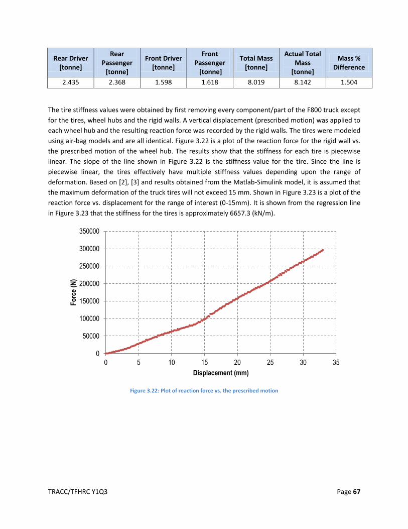
TRACC/TFHRC Y1Q3 Page 67
Rear Driver [tonne]
Rear Passenger
[tonne]
Front Driver [tonne]
Front Passenger [tonne]
Total Mass [tonne]
Actual Total Mass
[tonne]
Mass % Difference
2.435 2.368 1.598 1.618 8.019 8.142 1.504
The tire stiffness values were obtained by first removing every component/part of the F800 truck except
for the tires, wheel hubs and the rigid walls. A vertical displacement (prescribed motion) was applied to
each wheel hub and the resulting reaction force was recorded by the rigid walls. The tires were modeled
using air-bag models and are all identical. Figure 3.22 is a plot of the reaction force for the rigid wall vs.
the prescribed motion of the wheel hub. The results show that the stiffness for each tire is piecewise
linear. The slope of the line shown in Figure 3.22 is the stiffness value for the tire. Since the line is
piecewise linear, the tires effectively have multiple stiffness values depending upon the range of
deformation. Based on [2], [3] and results obtained from the Matlab-Simulink model, it is assumed that
the maximum deformation of the truck tires will not exceed 15 mm. Shown in Figure 3.23 is a plot of the
reaction force vs. displacement for the range of interest (0-15mm). It is shown from the regression line
in Figure 3.23 that the stiffness for the tires is approximately 6657.3 (kN/m).
Figure 3.22: Plot of reaction force vs. the prescribed motion
0
50000
100000
150000
200000
250000
300000
350000
0 5 10 15 20 25 30 35
Fo
rce
(N)
Displacement (mm)

TRACC/TFHRC Y1Q3 Page 68
Figure 3.23: Plot of force vs. displacement, for displacements less than 15 mm
The stiffness and damping values for the suspension of the F800 truck have yet to be obtained. Once
these are obtained, the gains for the controller can be found. Once the gains are found, the controller
can be evaluated in Matlab-Simulink, and further modification may be made in order to find the most
suitable values for the gains. A sub-routine in LS-DYNA will then be created to mimic the operation of
the controllable EMSA. Simulations will be performed to compare the performance of the EMSA
suspension system with the passive suspension system.
3.2.2.4. References
1) Gupta, A.; Jendrzejczyk, J. A.; Mulcahy, T. M.; Hull, J. R.; “Design of Electromagnetic Shock
Absorbers”, International Journal of Mechanics and Materials in Design, Vol. 3, No. 3, 2007, pp.
285-291.
2) Gao, H.; Lam, J.; Wang, C.; “Multi-objective Control of Vehicle Active Suspension Systems Via
Load-dependent Controllers,” Journal of Sound and Vibration, Vol. 290, 2006, pp. 654-675.
3) Du, H.; Sze, K.Y.; Lam, J.; “Semi-active H[infinity] control of vehicle suspension with magneto-
rheological dampers”, Journal of Sound and Vibration, Vol. 283, No. 3-5, 2005, pp. 981-996.
3.3. A Coupling of CFD and CSM Codes for Scour Shape Prediction
3.3.1. Introduction
As detailed in Section 4 of the TRACC Y5Q3 Progress Report, TRACC CFD researchers have been
investigating approaches to simulate the formation of scour holes and have been enhancing the
y = 6657.3x - 4687.7 R² = 0.9951
0
20000
40000
60000
80000
100000
0 2 4 6 8 10 12 14
Forc
e (
N)
Displacement (mm)
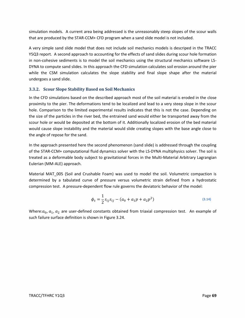
TRACC/TFHRC Y1Q3 Page 69
simulation models. A current area being addressed is the unreasonably steep slopes of the scour walls
that are produced by the STAR-CCM+ CFD program when a sand slide model is not included.
A very simple sand slide model that does not include soil mechanics models is descriped in the TRACC
Y5Q3 report. A second approach to accounting for the effects of sand slides during scour hole formation
in non-cohesive sediments is to model the soil mechanics using the structural mechanics software LS-
DYNA to compute sand slides. In this approach the CFD simulation calculates soil erosion around the pier
while the CSM simulation calculates the slope stability and final slope shape after the material
undergoes a sand slide.
3.3.2. Scour Slope Stability Based on Soil Mechanics
In the CFD simulations based on the described approach most of the soil material is eroded in the close
proximity to the pier. The deformations tend to be localized and lead to a very steep slope in the scour
hole. Comparison to the limited experimental results indicates that this is not the case. Depending on
the size of the particles in the river bed, the entrained sand would either be transported away from the
scour hole or would be deposited at the bottom of it. Additionally localized erosion of the bed material
would cause slope instability and the material would slide creating slopes with the base angle close to
the angle of repose for the sand.
In the approach presented here the second phenomenon (sand slide) is addressed through the coupling
of the STAR-CCM+ computational fluid dynamics solver with the LS-DYNA multiphysics solver. The soil is
treated as a deformable body subject to gravitational forces in the Multi-Material Arbitrary Lagrangian
Eulerian (MM-ALE) approach.
Material MAT_005 (Soil and Crushable Foam) was used to model the soil. Volumetric compaction is
determined by a tabulated curve of pressure versus volumetric strain defined from a hydrostatic
compression test. A pressure-dependent flow rule governs the deviatoric behavior of the model:
(
) (3.14)
Where: , , are user-defined constants obtained from triaxial compression test. An example of
such failure surface definition is shown in Figure 3.24.

TRACC/TFHRC Y1Q3 Page 70
Figure 3.24 Strength envelope in terms of yield surface- second invariant of deviatoric stress and pressure
The shear failure of the soil is occurring when the s defined in Equation (3.14) becomes zero. It means
that the stress state defined by the second stress invariant is located on the yield surface. This material
definition has a simple implication stating that if the confining pressure of the material is very low,
accordingly low shear stress would cause the material to fail. In the case of scour slope stability lack of
confinement of the sand is causing fluid-like flow of material.
3.3.3. Procedure Flowchart
The procedure consists of the following steps:
1. Run the analysis in STAR-CCM+ up to the point where the slope angle exceeds significantly the
natural angle of repose of the sand. (This is the state where deviatoric shear stress in the soil
can cause the slope to slide.)
2. Extract the shape of the scour hole in the NASTRAN file format.
3. Import the NASTRAN file to LS-PrePost – a pre and post processor for LS-DYNA.
4. Build a shell container with the shape of the scour for soil volume initialization in the LS-DYNA
simulation.
5. Analyze the slope stability problem using LS-DYNA MM-ALE capabilities.
6. Export final shape of the scour to the NASTRAN file that can be imported back to STAR-CCM+.
3.3.4. Simplifying Assumptions
The procedure of this coupling has several simplifications:
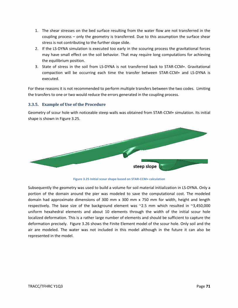
TRACC/TFHRC Y1Q3 Page 71
1. The shear stresses on the bed surface resulting from the water flow are not transferred in the
coupling process – only the geometry is transferred. Due to this assumption the surface shear
stress is not contributing to the further slope slide.
2. If the LS-DYNA simulation is executed too early in the scouring process the gravitational forces
may have small effect on the soil behavior. That may require long computations for achieving
the equilibrium position.
3. State of stress in the soil from LS-DYNA is not transferred back to STAR-CCM+. Gravitational
compaction will be occurring each time the transfer between STAR-CCM+ and LS-DYNA is
executed.
For these reasons it is not recommended to perform multiple transfers between the two codes. Limiting
the transfers to one or two would reduce the errors generated in the coupling process.
3.3.5. Example of Use of the Procedure
Geometry of scour hole with noticeable steep walls was obtained from STAR-CCM+ simulation. Its initial
shape is shown in Figure 3.25.
Figure 3.25 Initial scour shape based on STAR-CCM+ calculation
Subsequently the geometry was used to build a volume for soil material initialization in LS-DYNA. Only a
portion of the domain around the pier was modeled to save the computational cost. The modeled
domain had approximate dimensions of 300 mm x 300 mm x 750 mm for width, height and length
respectively. The base size of the background element was ~2.5 mm which resulted in ~3,450,000
uniform hexahedral elements and about 10 elements through the width of the initial scour hole
localized deformation. This is a rather large number of elements and should be sufficient to capture the
deformation precisely. Figure 3.26 shows the Finite Element model of the scour hole. Only soil and the
air are modeled. The water was not included in this model although in the future it can also be
represented in the model.

TRACC/TFHRC Y1Q3 Page 72
Figure 3.26 Finite Element model of the scour hole – initial state
The LS-DYNA simulation was performed on the TRACC high performance cluster using 8 compute nodes
(64 cores). It took approximately 12 hours to get to the state where no further movement of the soil was
registered. The final shape of the scour hole is shown in Figure 3.27.
Figure 3.27 Finite Element model of the scour hole – final state
Figure 3.28 shows side by side comparison of the initial and final shape of the scour hole in the LS-DYNA
simulation.

TRACC/TFHRC Y1Q3 Page 73
Figure 3.28 Comparison of the initial and the final shape of the scour hole

Argonne National Laboratory is a U.S. Department of Energy laboratory managed by UChicago Argonne, LLC
ENERGYU.S. DEPARTMENT OF
Energy Systems DivisionArgonne National Laboratory9700 South Cass Avenue, Bldg. 362Argonne, IL 60439-4815
www.anl.gov