Computed Tomography (part II) - Department of …eeweb.poly.edu/~yao/EL5823/CT_ch6_part2.pdf · Computed Tomography (part II) Yao Wang Polytechnic University, Brooklyn, NY 11201 Based

______ ______

Computed Tomography (part II)

Yao Wang Polytechnic University, Brooklyn, NY 11201

Based on J. L. Prince and J. M. Links, Medical Imaging Signals and Systems, and lecture notes by Prince. Figures are from the textbook.

Yao Wang, NYU-Poly EL5823/BE6203: CT-2 2

Last Lecture •  Instrumentation

–  CT Generations –  X-ray source and collimation –  CT detectors

•  Image Formation –  Line integrals –  Parallel Ray Reconstruction

•  Radon transform •  Back projection •  Filtered backprojection •  Convolution backprojection •  Implementation issues


This Lecture •  Review of Parallel Ray Projection and Reconstruction •  Practical implementation with samples •  Fan Beam Reconstruction •  Signal to Noise in CT


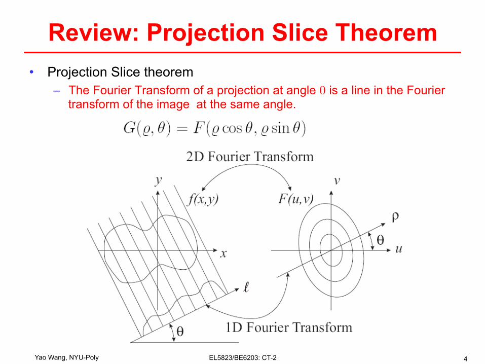
Review: Projection Slice Theorem •  Projection Slice theorem

–  The Fourier Transform of a projection at angle θ is a line in the Fourier transform of the image at the same angle.


Reconstruction Algorithm for Parallel Projections

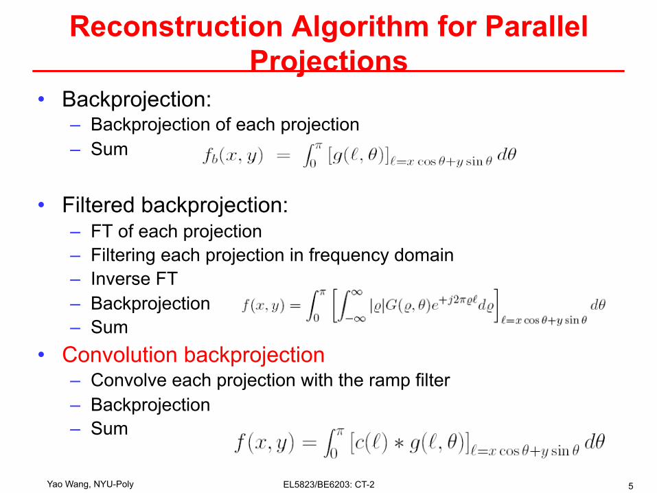
•  Backprojection: –  Backprojection of each projection –  Sum

•  Filtered backprojection: –  FT of each projection –  Filtering each projection in frequency domain –  Inverse FT –  Backprojection –  Sum

•  Convolution backprojection –  Convolve each projection with the ramp filter –  Backprojection –  Sum


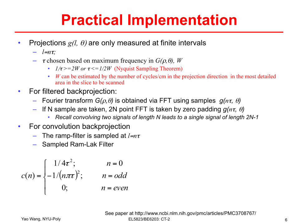
Practical Implementation •  Projections g(l, θ) are only measured at finite intervals

–  l=nτ; –  τ chosen based on maximum frequency in G(ρ,θ), W

•  1/τ >=2W or τ <=1/2W (Nyquist Sampling Theorem)

•  W can be estimated by the number of cycles/cm in the projection direction in the most detailed area in the slice to be scanned

•  For filtered backprojection: –  Fourier transform G(ρ,θ) is obtained via FFT using samples g(nτ, θ) –  If N sample are taken, 2N point FFT is taken by zero padding g(nτ, θ)

•  Recall convolving two signals of length N leads to a single signal of length 2N-1

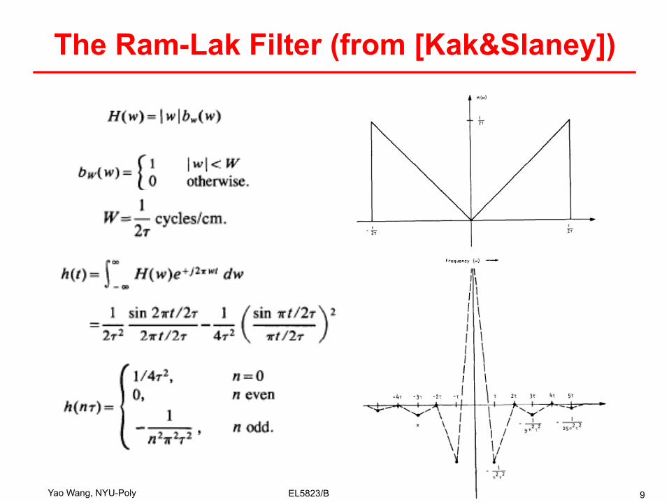
•  For convolution backprojection –  The ramp-filter is sampled at l=nτ –  Sampled Ram-Lak Filter

( )⎪⎩

⎪⎨

⎧

=

=−

=

=

evennoddnn

nnc

;0;/1

0;4/1)( 2

2

πτ

τ

See paper at http://www.ncbi.nlm.nih.gov/pmc/articles/PMC3708767/

Practical Implementation of Filter Backprojection


Shi and Luo BioMedical Engineering OnLine 2013, 12:50 Page 3 of 15http://www.biomedical-engineering-online.com/content/12/1/50

Then the unknown f (x, y) can be reconstructed by the inverse Fourier transform (IFT)or the dual Radon transform as following

f̂ (x, y) =! !

0

! !

"!F(" cos # , " sin #)|"| exp(i2!"(x cos # + y sin #))d"d#

=! !

0

! !

"!S# (")|"| exp(i2!"t)d"d# ,

where f̂ (x, y) denotes the reconstructed image; t = x cos # + y sin # ; |"| is known as

“ramp” filter in the frequency domain. It is well-known that f̂ (x, y) will be identical withf (x, y) almost everywhere according to the properties of FT and IFT.

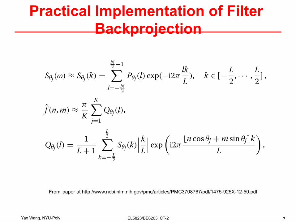
In practice, the projection data and reconstructed images have to be discretized torecord, calculate and display. For the discrete projection data, P#j(l), l # [ "N

2 , · · · , N2 ], the

discrete Fourier transform (DFT) and inverse DFT (IDFT) are employed to approximate(continuous) FT and IFT, respectively. They are

S#j(") $ S#j(k) =N2 "1"

l=" N2

P#j(l) exp("i2!lkL ), k # [ "L

2 , · · · , L2 ] ,

f̂ (n, m) $ !

K

K"

j=1Q#j(l),

Q#j(l) = 1L + 1

L2"

k=" L2

S#j(k)###kL

### exp$

i2!%n cos #j + m sin #j&k

L

%,

(2)

where N is a positive even integer denotes the number of projection data; L is an eveninteger that is equal to or larger than the maximum number of the discrete projectiondata at all directions; %x& denotes the nearest integer of x; #j, j # [1, · · · , K], denote thediscretized scanning angle, and K is the number of the scanning angles. The discretizedramp filter, | k

L |, is named as the reconstruction filter in this paper.For the continuous systems, Radon and inverse Radon transforms are solid and per-

fect in the mathematics principle [8-10]. However, it necessarily produces non-negligibledegradation when the projection data are discrete (finite) and Radon and inverse Radontransforms have to be discretized in calculation. Many scholars have studied this prob-lem. In [15], a multilevel back-projection method had been presented to improve thecomputational speed. The point-spread-function (PSF) convolution techniques had beenproposed to reduce blurring. By those approaches the image quality was similar with orsuperior to that using the standard FBP technique. In [16], the spline interpolation andramp filtering had been combined to improve the standard FBP algorithm, by which theimage quality could also be improved somewhat.

The question can be summarized as how to reduce the degradation caused by the dis-cretizing process. Since the degradation cannot be removed completely, the questioncan also be simplified as how to design the optimal reconstruction filter for the discreteinverse Radon transform. In this paper, we try to solve this question in a quite differ-ent way. First, the discrete image model and discrete projection model are employed insimulating the scanning procedure. The DFT of projection data is regarded as a special

From paper at http://www.ncbi.nlm.nih.gov/pmc/articles/PMC3708767/pdf/1475-925X-12-50.pdf

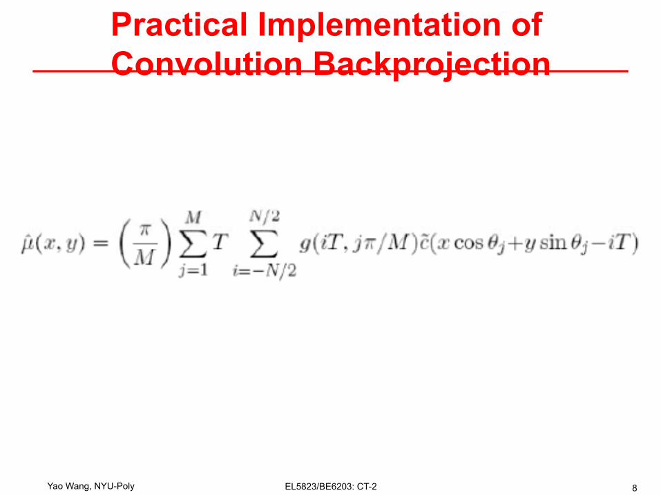
Practical Implementation of Convolution Backprojection



The Ram-Lak Filter (from [Kak&Slaney])


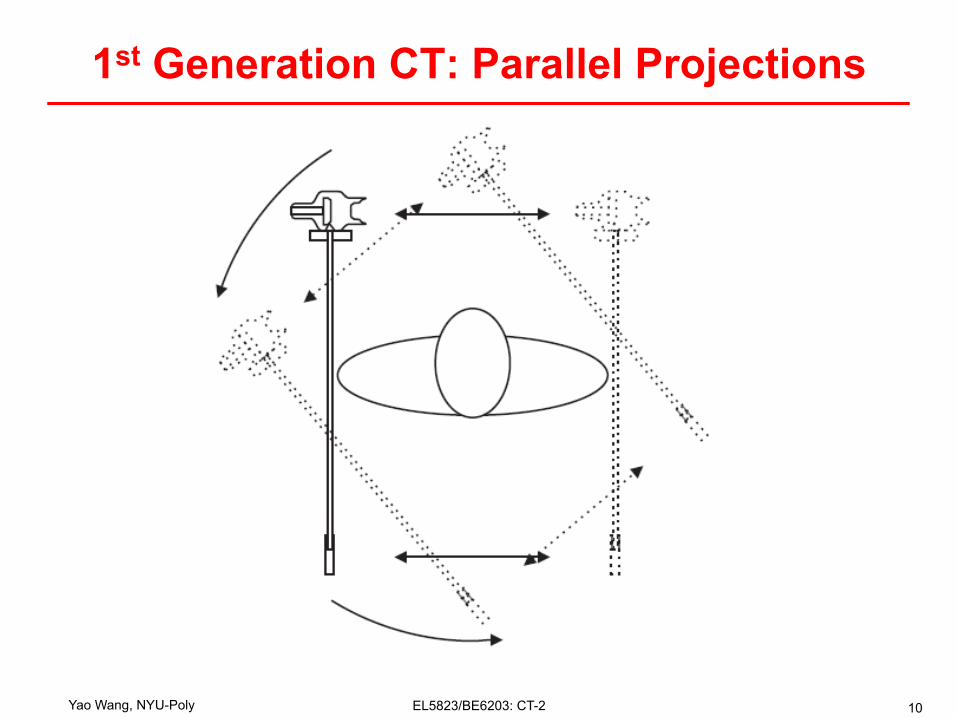
1st Generation CT: Parallel Projections


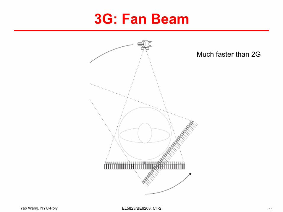
3G: Fan Beam

Much faster than 2G


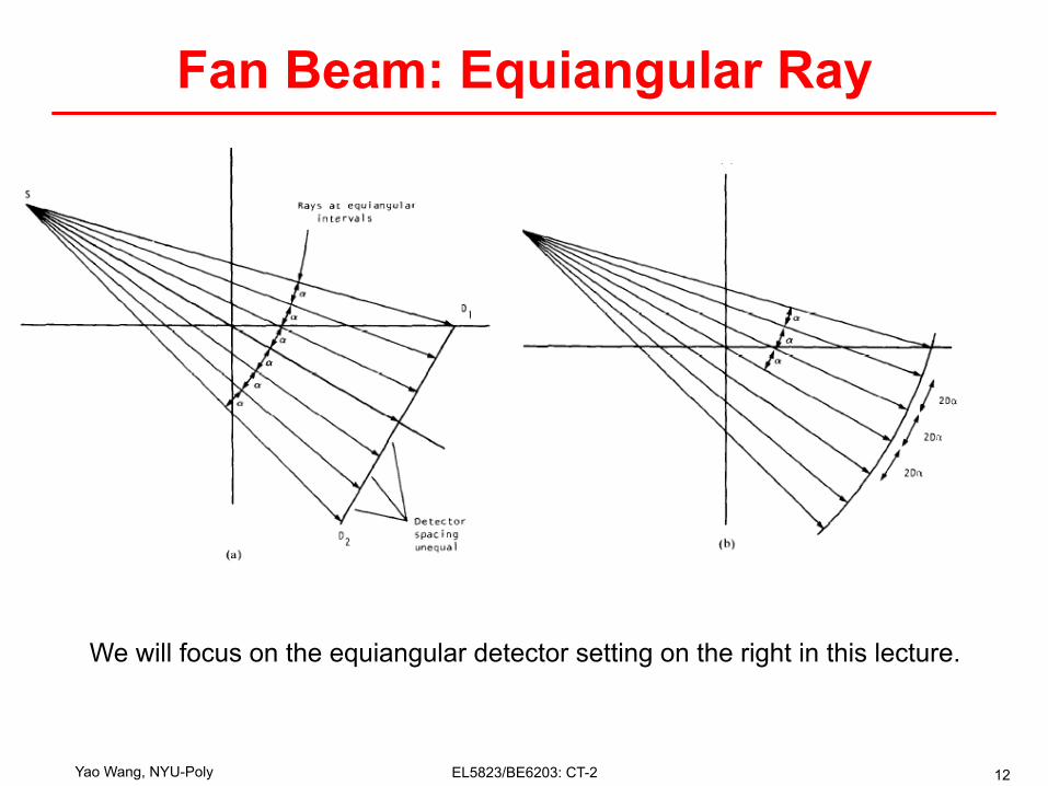
Fan Beam: Equiangular Ray

We will focus on the equiangular detector setting on the right in this lecture.


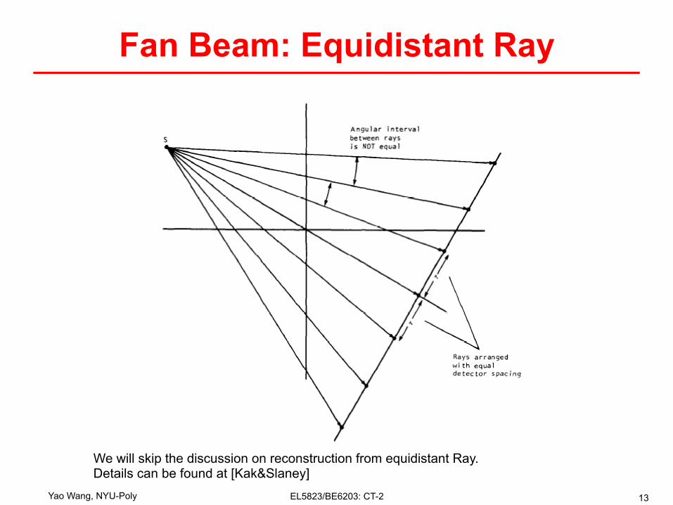
Fan Beam: Equidistant Ray

We will skip the discussion on reconstruction from equidistant Ray. Details can be found at [Kak&Slaney]


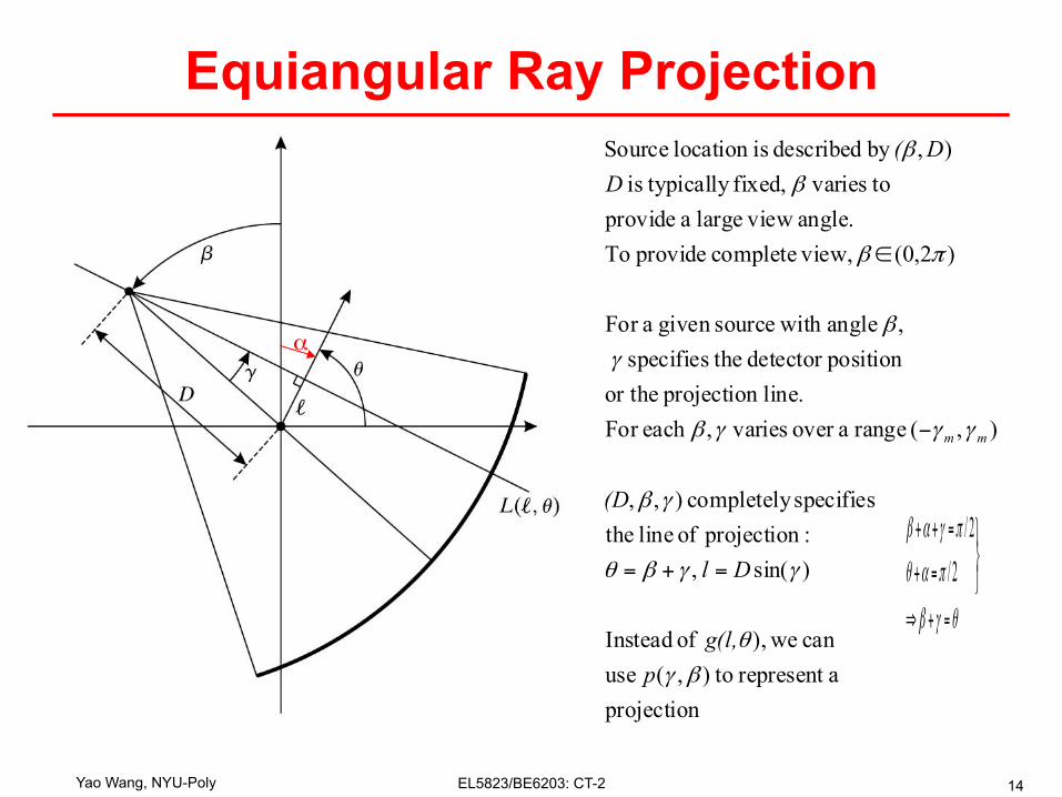
Equiangular Ray Projection

projection arepresent to),( use

can we), of Instead

)sin(,:projection of line the

specifies completely ),,

),( range aover varies,each For line. projection or the

position detector thespecifies , angle with sourcegiven aFor

)2,0( view,complete provide Toangle. viewlarge a provide

to varies fixed, typicallyis ),by described islocation Source

βγ

θ

γγβθ

γβ

γγγβ

γ

β

πβ

β

β

pg(l,

Dl

(D

DD(

mm

=+=

−

∈

θγβ

παθ

πγαβ

=+⇒⎭⎬⎫

=+

=++

2/2/

α


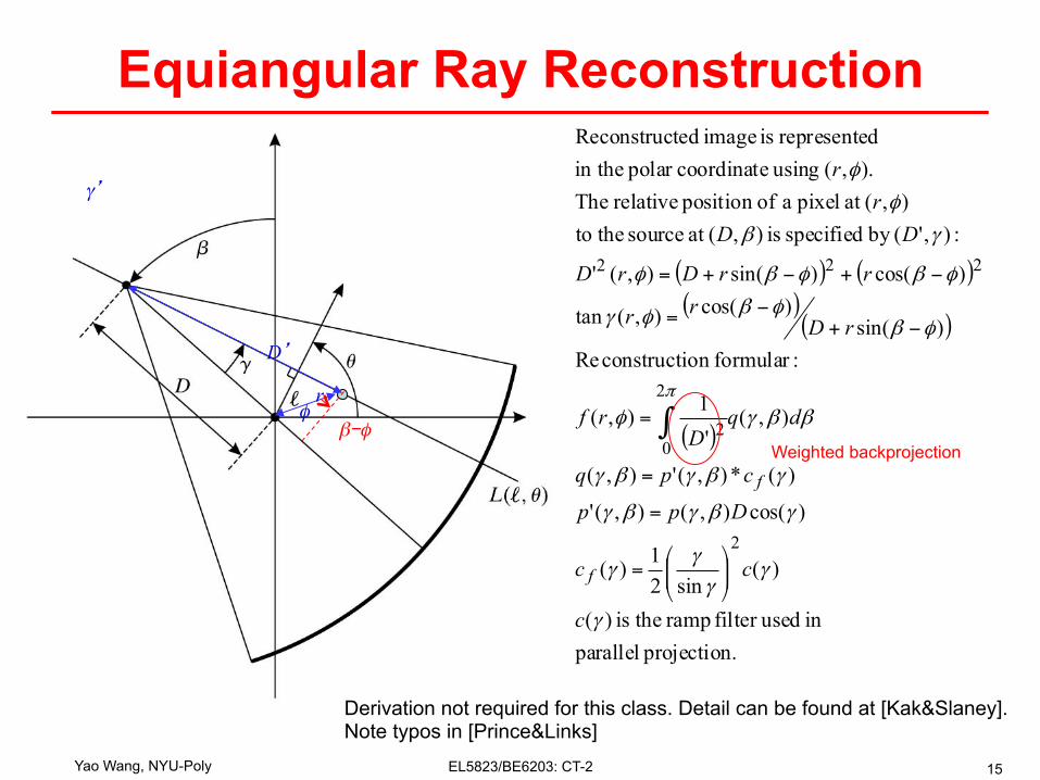
Equiangular Ray Reconstruction

D’

r φ

( ) ( )( )

( )

( )

.projection parallelin usedfilter ramp theis )(

)(sin2

1)(

)cos(),(),('

)(*),('),(

),('

1),(

:formularon constructiRe)sin(

)cos(),(tan

)cos()sin(),('

:),'(by specified is ),(at source theto),(at pixel a ofposition relative The

).,( using coordinatepolar in thedrepresente is image tedReconstruc

2

2

02

222

γ

γγ

γγ

γβγβγ

γβγβγ

ββγφ

φβφβφγ

φβφβφ

γβ

φ

φ

π

c

cc

Dpp

cpq

dqD

rf

rDrr

rrDrD

DDr

r

f

f

⎟⎟⎠

⎞⎜⎜⎝

⎛=

=

=

=

−+−=

−+−+=

∫

γ’

Derivation not required for this class. Detail can be found at [Kak&Slaney]. Note typos in [Prince&Links]

β-φ Weighted backprojection


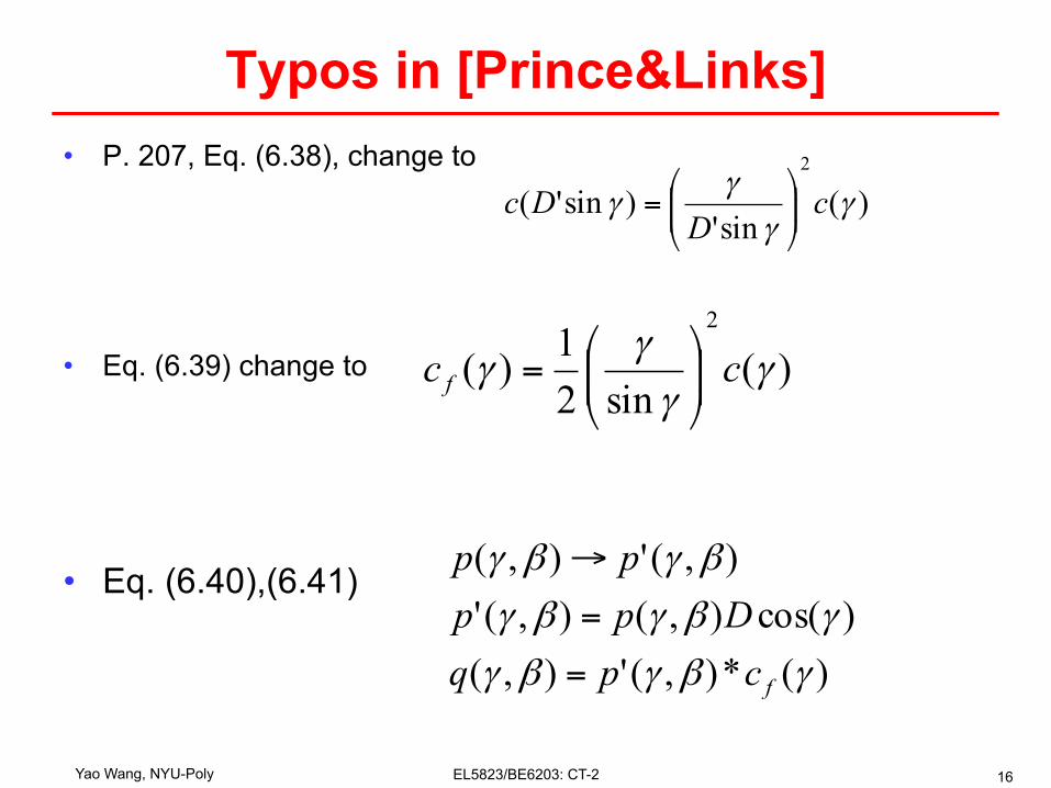
Typos in [Prince&Links] •  P. 207, Eq. (6.38), change to

•  Eq. (6.39) change to

•  Eq. (6.40),(6.41)

)(sin'

)sin'(2

γγ

γγ c

DDc ⎟⎟

⎠

⎞⎜⎜⎝

⎛=

)(sin2

1)(2

γγ

γγ cc f ⎟⎟

⎠

⎞⎜⎜⎝

⎛=

)(*),('),()cos(),(),('

),('),(

γβγβγ

γβγβγ

βγβγ

fcpqDpp

pp

=

=

→


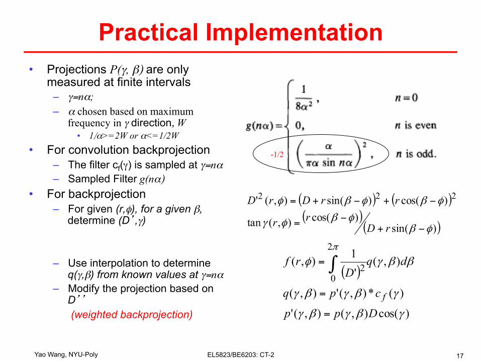
Practical Implementation •  Projections P(γ, β) are only

measured at finite intervals –  γ=nα; –  α chosen based on maximum

frequency in γ direction, W •  1/α>=2W or α<=1/2W

•  For convolution backprojection –  The filter cf(γ) is sampled at γ=nα –  Sampled Filter g(nα)

•  For backprojection –  For given (r,φ), for a given β,

determine (D’,γ)

–  Use interpolation to determine q(γ,β) from known values at γ=nα

–  Modify the projection based on D’’

(weighted backprojection)

( ) ( )( )

( ))sin()cos(),(tan

)cos()sin(),(' 222

φβφβφγ

φβφβφ

−+−=

−+−+=

rDrr

rrDrD

( )

)cos(),(),('

)(*),('),(

),('1),(

2

02

γβγβγ

γβγβγ

ββγφπ

Dpp

cpq

dqD

rf

f

=

=

= ∫

-1/2


Matlab Functions for Fan Beam CT •  Relevant functions:

–  fanbeam(), ifanbeam()


CT Quality Evaluation •  Blurring Effect •  SNR


Effect of Area Detector •  Practical detector integrates the detected photons over

an area •  Mathematically, the detector can be characterized by an

indicator function s(l) (aka impulse response) •  The measured projection g’(l,θ) is related to “real”

projection g(l,θ) by –  g’(l,θ)= g(l,θ) * s(l) –  G’(ρ,θ)= G(ρ,θ) S(ρ)


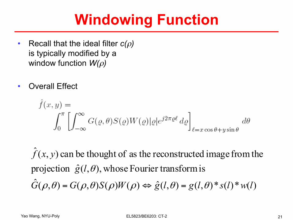
Windowing Function •  Recall that the ideal filter c(ρ)

is typically modified by a window function W(ρ)

•  Overall Effect

)(*)(*),(),(ˆ)()(),(),(ˆ is ansformFourier tr whose),,(ˆ projection

thefrom image tedreconstruc theas of thought becan ),(ˆ

lwlslglgWSGG

lgyxf

θθρρθρθρ

θ

=⇔=


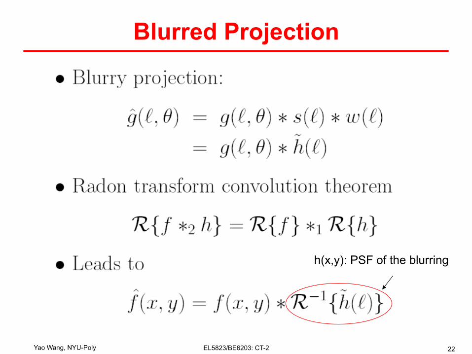
Blurred Projection

h(x,y): PSF of the blurring


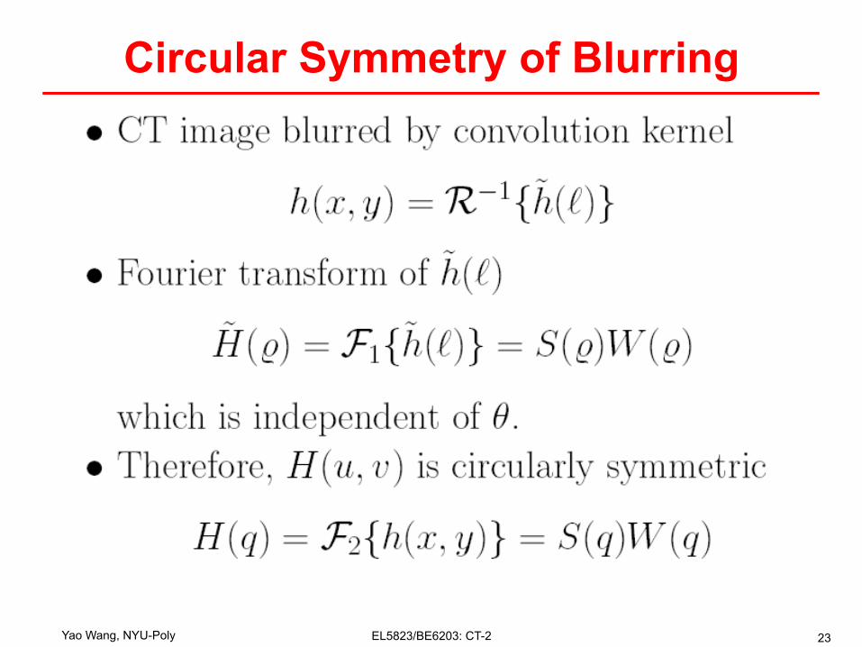
Circular Symmetry of Blurring


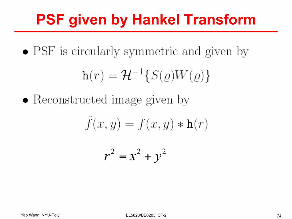
PSF given by Hankel Transform

222 yxr +=


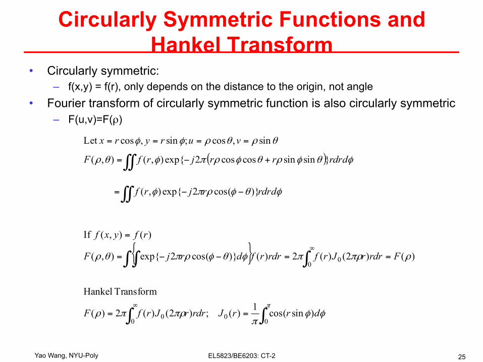
Circularly Symmetric Functions and Hankel Transform

•  Circularly symmetric: –  f(x,y) = f(r), only depends on the distance to the origin, not angle

•  Fourier transform of circularly symmetric function is also circularly symmetric –  F(u,v)=F(ρ)

( )

{ }

∫∫

∫∫ ∫

∫∫

∫∫

==

==−−=

=

−−=

+−=

====

∞

∞

πφφ

ππρπρ

ρπρπφθφρπθρ

φθφρπφ

φθφρθφρπφθρ

θρθρφφ

00

00

00

)sincos(1)(;)2()(2)(

Transform Hankel

)()2()(2)()}cos(2exp{),(

)(),( If

)}cos(2exp{),(

}sinsincoscos2exp{),(),(

sin,cos;sin,cosLet

drrJrdrrJrfF

FrdrrJrfrdrrfdrjF

rfyxf

rdrdrjrf

rdrdrrjrfF

vuryrx


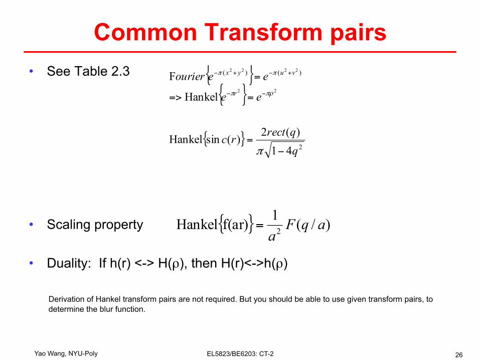
Common Transform pairs •  See Table 2.3

•  Scaling property

•  Duality: If h(r) <-> H(ρ), then H(r)<->h(ρ)

{ } )/(1f(ar)Hankel 2 aqFa

=

{ }{ }

{ }2

)()(

41)(2)(sinHankel

Hankel

F22

2222

qqrectrc

ee

eeourierr

vuyx

−=

==>

=−−

+−+−

π

πρπ

ππ

Derivation of Hankel transform pairs are not required. But you should be able to use given transform pairs, to determine the blur function.


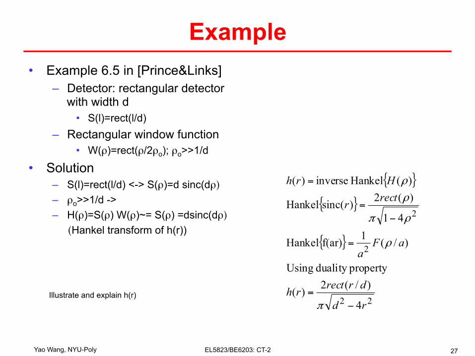
Example •  Example 6.5 in [Prince&Links]

–  Detector: rectangular detector with width d

•  S(l)=rect(l/d) –  Rectangular window function

•  W(ρ)=rect(ρ/2ρo); ρo>>1/d

•  Solution –  S(l)=rect(l/d) <-> S(ρ)=d sinc(dρ)

–  ρo>>1/d -> –  H(ρ)=S(ρ) W(ρ)~= S(ρ) =dsinc(dρ)

(Hankel transform of h(r))

{ }

{ }

{ }

22

2

2

4

)/(2)(

propertyduality Using

)/(1f(ar)Hankel

41

)(2)(sincHankel

)(Hankel inverse)(

rd

drrectrh

aFa

rectr

Hrh

−=

=

−=

=

π

ρ

ρπ

ρ

ρ

Illustrate and explain h(r)


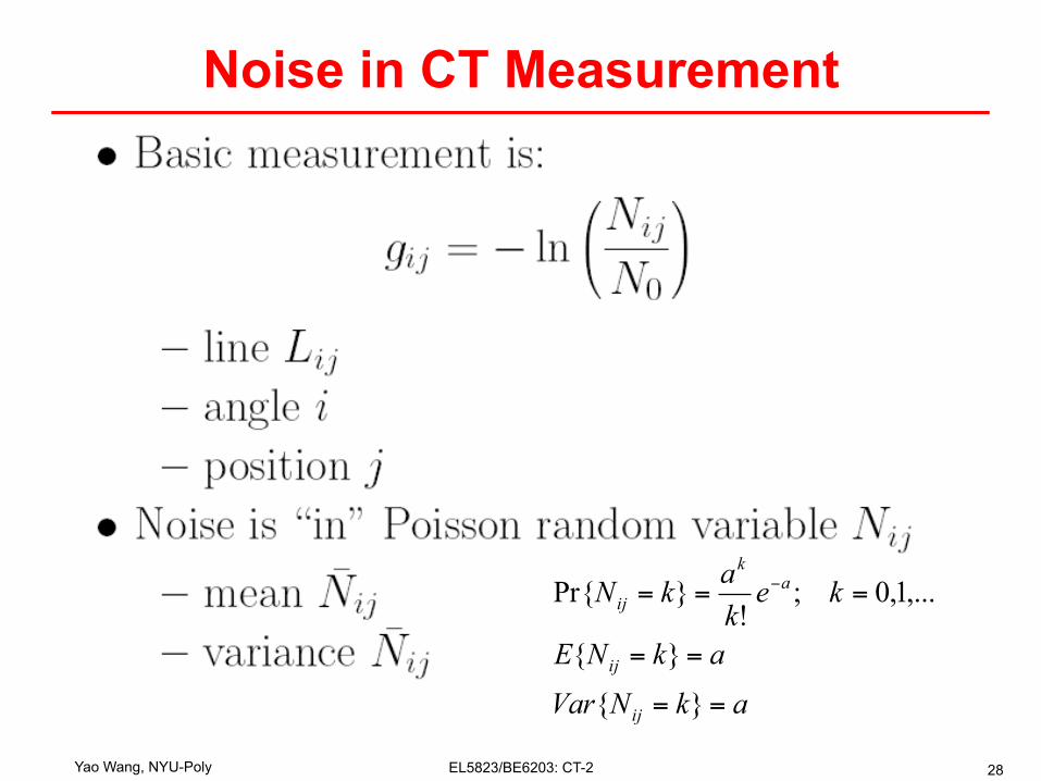
Noise in CT Measurement

akNVarakNE

kekakN

ij

ij

ak

ij

==

==

=== −

}{

}{

,...1,0;!

}Pr{


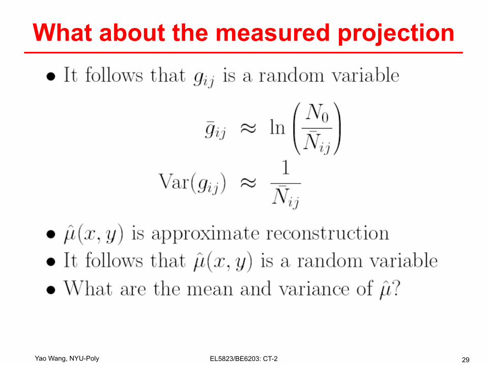
What about the measured projection


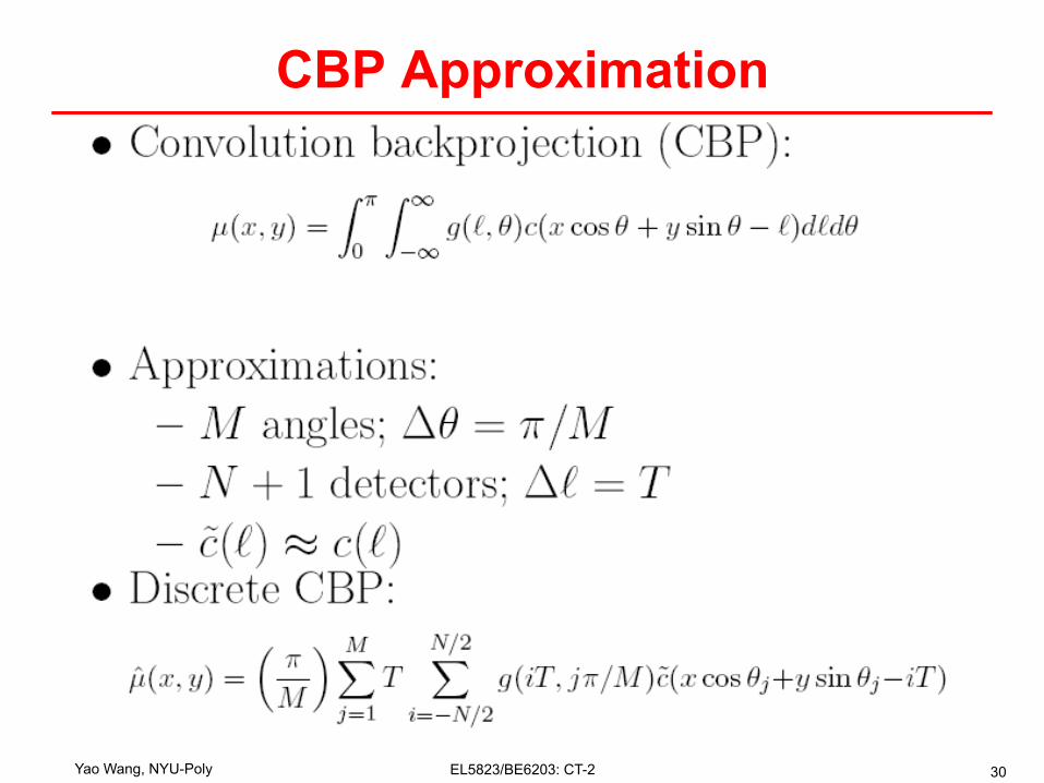
CBP Approximation


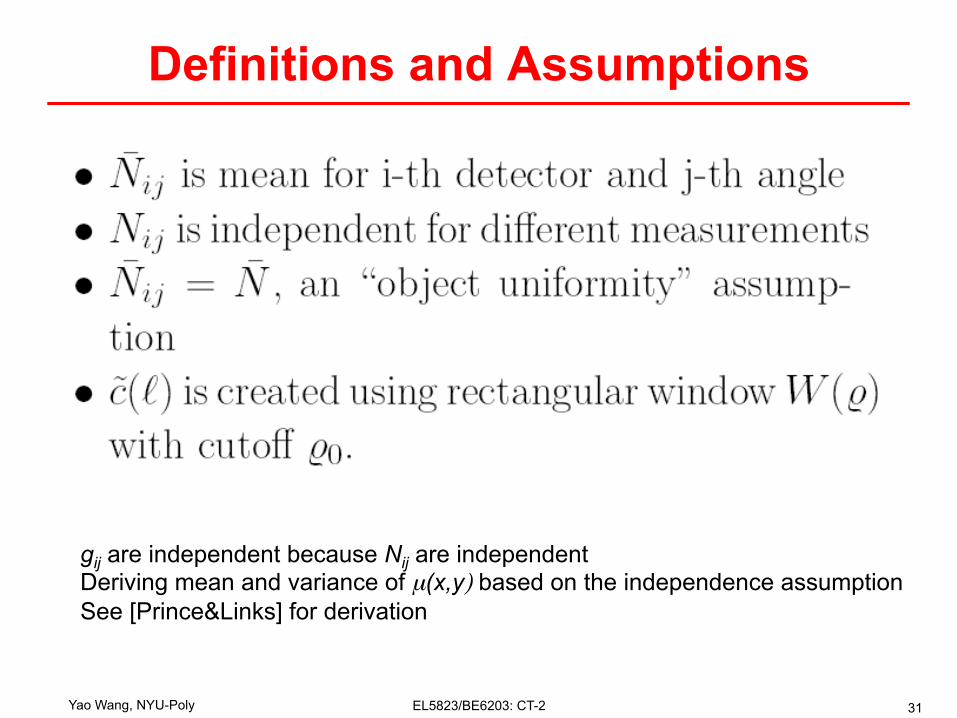
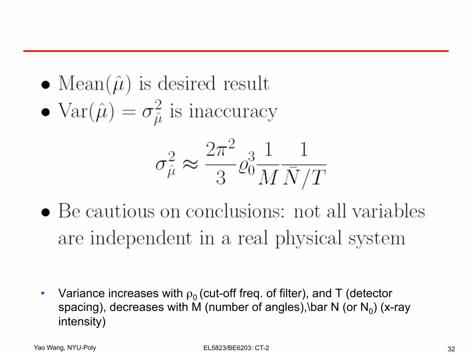
Definitions and Assumptions

gij are independent because Nij are independent Deriving mean and variance of µ(x,y) based on the independence assumption See [Prince&Links] for derivation


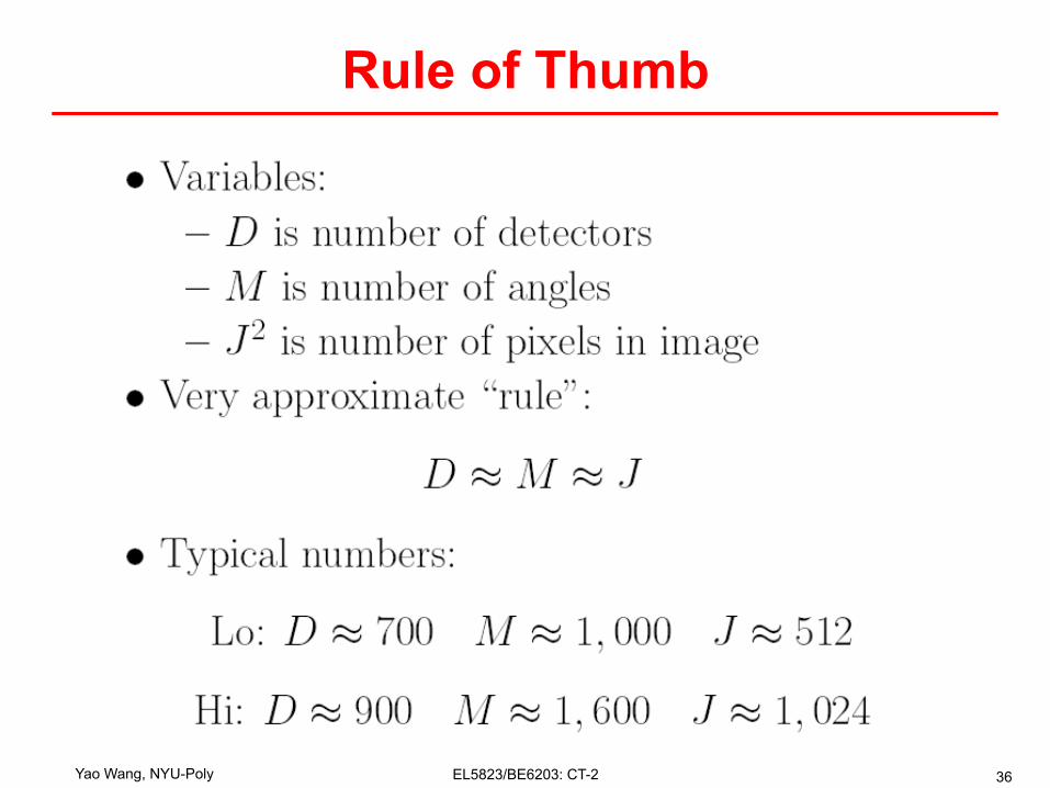
•  Variance increases with ρ0 (cut-off freq. of filter), and T (detector spacing), decreases with M (number of angles),\bar N (or N0) (x-ray intensity)


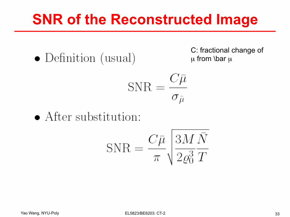
SNR of the Reconstructed Image

C: fractional change of µ from \bar µ


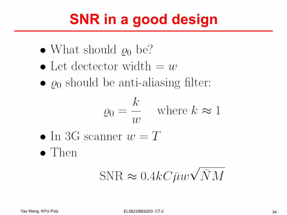
SNR in a good design


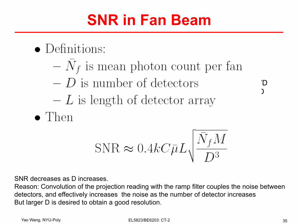
SNR in Fan Beam

N=Nf/D w=L/D

SNR decreases as D increases. Reason: Convolution of the projection reading with the ramp filter couples the noise between detectors, and effectively increases the noise as the number of detector increases But larger D is desired to obtain a good resolution.


Rule of Thumb


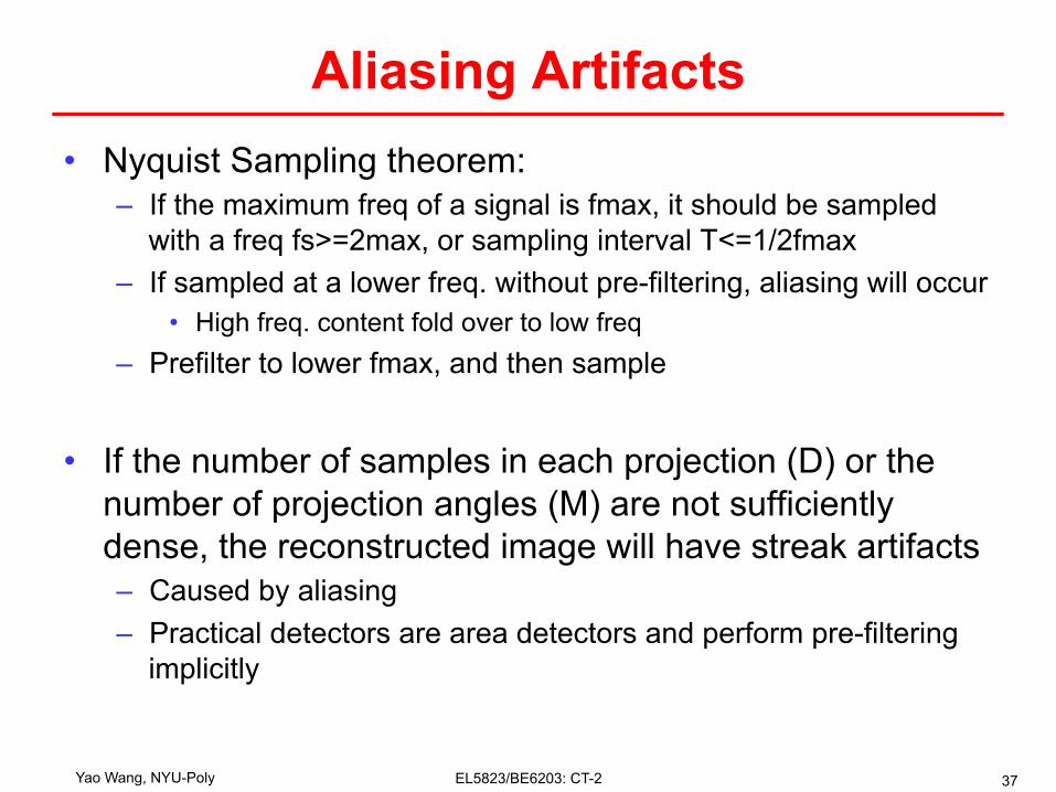
Aliasing Artifacts •  Nyquist Sampling theorem:

–  If the maximum freq of a signal is fmax, it should be sampled with a freq fs>=2max, or sampling interval T<=1/2fmax

–  If sampled at a lower freq. without pre-filtering, aliasing will occur •  High freq. content fold over to low freq

–  Prefilter to lower fmax, and then sample

•  If the number of samples in each projection (D) or the number of projection angles (M) are not sufficiently dense, the reconstructed image will have streak artifacts –  Caused by aliasing –  Practical detectors are area detectors and perform pre-filtering

implicitly


From [Kak&Slaney] Fig. 5.1


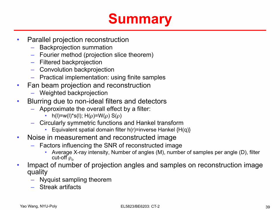
Summary •  Parallel projection reconstruction

–  Backprojection summation –  Fourier method (projection slice theorem) –  Filtered backprojection –  Convolution backprojection –  Practical implementation: using finite samples

•  Fan beam projection and reconstruction –  Weighted backprojection

•  Blurring due to non-ideal filters and detectors –  Approximate the overall effect by a filter:

•  h(l)=w(l)*s(l); H(ρ)=W(ρ) S(ρ) –  Circularly symmetric functions and Hankel transform

•  Equivalent spatial domain filter h(r)=inverse Hankel {H(q)} •  Noise in measurement and reconstructed image

–  Factors influencing the SNR of reconstructed image •  Average X-ray intensity, Number of angles (M), number of samples per angle (D), filter

cut-off ρo

•  Impact of number of projection angles and samples on reconstruction image quality

–  Nyquist sampling theorem –  Streak artifacts


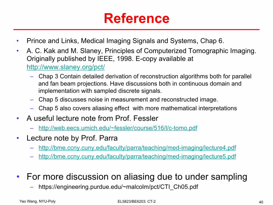
Reference •  Prince and Links, Medical Imaging Signals and Systems, Chap 6. •  A. C. Kak and M. Slaney, Principles of Computerized Tomographic Imaging.

Originally published by IEEE, 1998. E-copy available at http://www.slaney.org/pct/

–  Chap 3 Contain detailed derivation of reconstruction algorithms both for parallel and fan beam projections. Have discussions both in continuous domain and implementation with sampled discrete signals.

–  Chap 5 discusses noise in measurement and reconstructed image. –  Chap 5 also covers aliasing effect with more mathematical interpretations

•  A useful lecture note from Prof. Fessler –  http://web.eecs.umich.edu/~fessler/course/516/l/c-tomo.pdf

•  Lecture note by Prof. Parra –  http://bme.ccny.cuny.edu/faculty/parra/teaching/med-imaging/lecture4.pdf –  http://bme.ccny.cuny.edu/faculty/parra/teaching/med-imaging/lecture5.pdf

•  For more discussion on aliasing due to under sampling –  https://engineering.purdue.edu/~malcolm/pct/CTI_Ch05.pdf


Homework •  Reading:

–  Prince and Links, Medical Imaging Signals and Systems, Chap 6, Sec.6.3.4-6.5

•  Note down all the corrections for Ch. 6 on your copy of the textbook based on the provided errata.

•  Problems for Chap 6 of the text book: –  P.6.9 –  P.6.10 (part e is not required) –  P.6.13.

•  Hint: solution for part (a) should be

–  P.6.17 –  P.6.19 –  P.6.20

( )( )

⎪⎩

⎪⎨

⎧

≤≤−

≤≤−+

=

otherwiseallalala

lg0

2/02/302/2/3

)60,( µ

µ


Computer Assignment 1.  Learn how do ‘fanbeam’.’ifanbeam’ work; summarize their

functionalities. Type ‘demos’ on the command line, then select ‘toolbox -> image processing -> transform -> reconstructing an image from projection data’. Alternatively, you can use ‘help’ for each particular function.

2.  Write a MATLAB program that 1) generate a phantom image (you can use a standard phantom provided by MATLAB or construct your own), 2) produce equiangular fan beam projections; 3) reconstruct the phantom using filtered backprojection algorithm; Your program should allow the user to specify the number of fan beams, and the number of projections per fan beam, the angular spacing between the projections. Run your program with different number of projections for the same view angle, and with different view angles, and compare the quality. Use the same filter and interpolation algorithm for all the comparisons. Compare the reconstructed image quality obtained with different number of view angles and number of projections per view angle. Also, compare the image quality with those obtained with parallel projections for the same phantom image when the same total number of measurements are used (from your last assignment). You can use the “fanbeam()” and “ifanbeam()” functions in MATLAB.

Documents

Computed Tomography (part II) - Department of …eeweb.poly.edu/~yao/EL5823/CT_ch6_part2.pdf · Computed Tomography (part II) Yao Wang Polytechnic University, Brooklyn, NY 11201 Based