Embed Size (px)
Citation preview
May 2010 Computer Arithmetic, Implementation Topics Slide 1
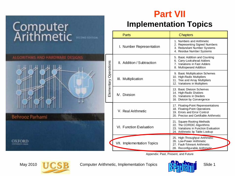
Part VIIImplementation Topics
Number Representation Numbers and Arithmetic Representing Signed Numbers Redundant Number Systems Residue Number Systems
Addition / Subtraction Basic Addition and Counting Carry-Lookahead Adders Variations in Fast Adders Multioperand Addition
Multiplication Basic Multiplication Schemes High-Radix Multipliers Tree and Array Multipliers Variations in Multipliers
Division Basic Division Schemes High-Radix Dividers Variations in Dividers Division by Convergence
Real Arithmetic Floating-Point Reperesentations Floating-Point Operations Errors and Error Control Precise and Certifiable Arithmetic
Function Evaluation Square-Rooting Methods The CORDIC Algorithms Variations in Function Evaluation Arithmetic by Table Lookup
Implementation Topics High-Throughput Arithmetic Low-Power Arithmetic Fault-Tolerant Arithmetic Past, Present, and Future
Parts Chapters
I.
II.
III.
IV.
V.
VI.
VII.
1. 2. 3. 4.
5. 6. 7. 8.
9. 10. 11. 12.
25. 26. 27. 28.
21. 22. 23. 24.
17. 18. 19. 20.
13. 14. 15. 16.
Ele
men
tary
Ope
ratio
ns
28. Reconfigurable Arithmetic
Appendix: Past, Present, and Future
May 2010 Computer Arithmetic, Implementation Topics Slide 2
About This Presentation
Edition Released Revised Revised Revised RevisedFirst Jan. 2000 Sep. 2001 Sep. 2003 Oct. 2005 Dec. 2007
Second May 2010
This presentation is intended to support the use of the textbookComputer Arithmetic: Algorithms and Hardware Designs (Oxford U. Press, 2nd ed., 2010, ISBN 978-0-19-532848-6). It is updated regularly by the author as part of his teaching of the graduate course ECE 252B, Computer Arithmetic, at the University of California, Santa Barbara. Instructors can use these slides freely in classroom teaching and for other educational purposes. Unauthorized uses are strictly prohibited. © Behrooz Parhami
May 2010 Computer Arithmetic, Implementation Topics Slide 3
VII Implementation Topics
Topics in This PartChapter 25 High-Throughput ArithmeticChapter 26 Low-Power ArithmeticChapter 27 Fault-Tolerant ArithmeticChapter 28 Reconfigurable Arithmetic
Sample advanced implementation methods and tradeoffs• Speed/ latency is seldom the only concern• We also care about throughput, size, power/energy• Fault-induced errors are different from arithmetic errors• Implementation on Programmable logic devices
May 2010 Computer Arithmetic, Implementation Topics Slide 4
May 2010 Computer Arithmetic, Implementation Topics Slide 5
25 High-Throughput ArithmeticChapter Goals
Learn how to improve the performance ofan arithmetic unit via higher throughputrather than reduced latency
Chapter HighlightsTo improve overall performance, one must
• Look beyond individual operations• Trade off latency for throughput
For example, a multiply may take 20 cycles,but a new one can begin every cycle
Data availability and hazards limit the depth
May 2010 Computer Arithmetic, Implementation Topics Slide 6
High-Throughput Arithmetic: Topics
Topics in This Chapter
25.1 Pipelining of Arithmetic Functions
25.2 Clock Rate and Throughput
25.3 The Earle Latch
25.4 Parallel and Digit-Serial Pipelines
25.5 On-Line of Digit-Pipelined Arithmetic
25.6 Systolic Arithmetic Units
May 2010 Computer Arithmetic, Implementation Topics Slide 7
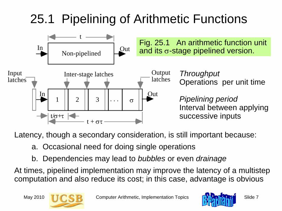
25.1 Pipelining of Arithmetic Functions
ThroughputOperations per unit time
Pipelining periodInterval between applying successive inputs
In Out1 . . .
Inter-stage latchesInput latches
Output latches
In OutNon-pipelined
t/ +τ
2 σ3
σt + στ
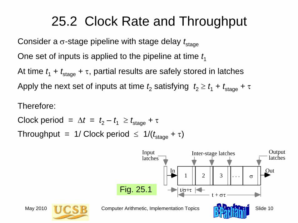
tFig. 25.1 An arithmetic function unit and its σ-stage pipelined version.
Latency, though a secondary consideration, is still important because:a. Occasional need for doing single operationsb. Dependencies may lead to bubbles or even drainage
At times, pipelined implementation may improve the latency of a multistep computation and also reduce its cost; in this case, advantage is obvious
May 2010 Computer Arithmetic, Implementation Topics Slide 8
Analysis of Pipelining Throughput
In Out1 . . .
Inter-stage latchesInput latches
Output latches
In OutNon-pipelined
t/ +τ
2 σ3
σt + στ
t
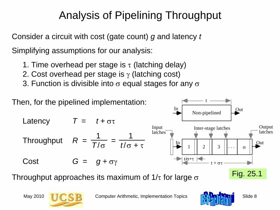
Consider a circuit with cost (gate count) g and latency t
Simplifying assumptions for our analysis:
1. Time overhead per stage is τ (latching delay)2. Cost overhead per stage is γ (latching cost)3. Function is divisible into σ equal stages for any σ
Then, for the pipelined implementation:
Latency T = t + στ
1 1Throughput R = = T / σ t / σ + τ
Cost G = g + σγ
Throughput approaches its maximum of 1/τ for large σ Fig. 25.1
May 2010 Computer Arithmetic, Implementation Topics Slide 9
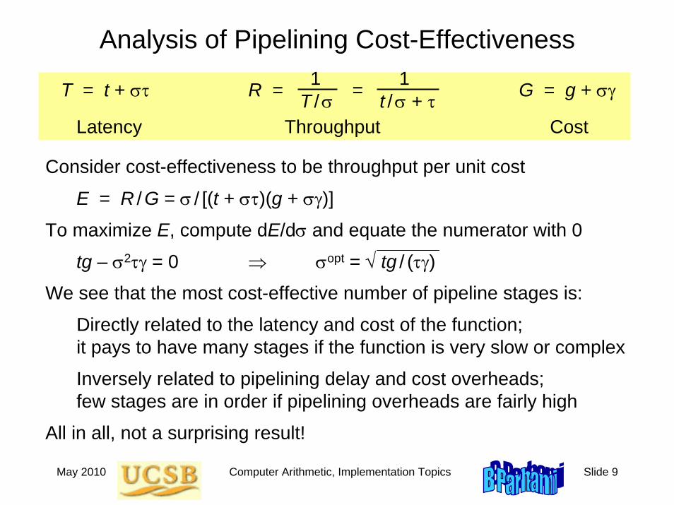
Analysis of Pipelining Cost-Effectiveness1 1T = t + στ R = = G = g + σγT / σ t / σ + τ
Latency Throughput Cost
Consider cost-effectiveness to be throughput per unit cost
E = R /G = σ / [(t + στ)(g + σγ)]
To maximize E, compute dE/dσ and equate the numerator with 0
tg – σ2τγ = 0 ⇒ σopt = √ tg / (τγ)
We see that the most cost-effective number of pipeline stages is:
Directly related to the latency and cost of the function; it pays to have many stages if the function is very slow or complex
Inversely related to pipelining delay and cost overheads;few stages are in order if pipelining overheads are fairly high
All in all, not a surprising result!
May 2010 Computer Arithmetic, Implementation Topics Slide 10
In Out1 . . .
Inter-stage latchesInput latches
Output latches
In OutNon-pipelined
t/ +τ
2 σ3
σt + στ
t
25.2 Clock Rate and ThroughputConsider a σ-stage pipeline with stage delay tstage
One set of inputs is applied to the pipeline at time t1At time t1 + tstage + τ, partial results are safely stored in latches
Apply the next set of inputs at time t2 satisfying t2 ≥ t1 + tstage + τ
Therefore:
Clock period = Δt = t2 – t1 ≥ tstage + τ
Throughput = 1/ Clock period ≤ 1/(tstage + τ)
Fig. 25.1
May 2010 Computer Arithmetic, Implementation Topics Slide 11
In Out1 . . .
Inter-stage latchesInput latches
Output latches
In OutNon-pipelined
t/ +τ
2 σ3
σt + στ
t
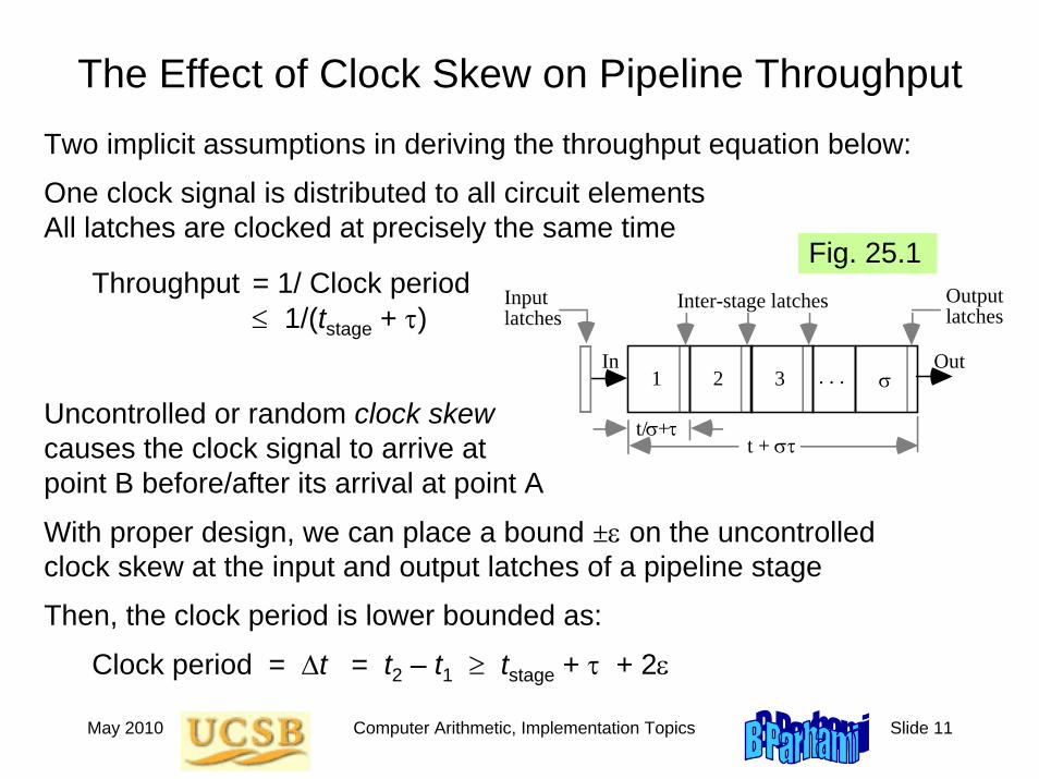
The Effect of Clock Skew on Pipeline ThroughputTwo implicit assumptions in deriving the throughput equation below:
One clock signal is distributed to all circuit elements All latches are clocked at precisely the same time
Throughput = 1/ Clock period ≤ 1/(tstage + τ)
Fig. 25.1
Uncontrolled or random clock skewcauses the clock signal to arrive at point B before/after its arrival at point A
With proper design, we can place a bound ±ε on the uncontrolled clock skew at the input and output latches of a pipeline stage
Then, the clock period is lower bounded as:
Clock period = Δt = t2 – t1 ≥ tstage + τ + 2ε
May 2010 Computer Arithmetic, Implementation Topics Slide 12
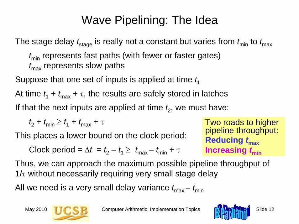
Wave Pipelining: The Idea
The stage delay tstage is really not a constant but varies from tmin to tmax
tmin represents fast paths (with fewer or faster gates) tmax represents slow paths
Suppose that one set of inputs is applied at time t1At time t1 + tmax + τ, the results are safely stored in latches
If that the next inputs are applied at time t2, we must have:
t2 + tmin ≥ t1 + tmax + τ
This places a lower bound on the clock period:
Clock period = Δt = t2 – t1 ≥ tmax – tmin + τ
Thus, we can approach the maximum possible pipeline throughput of 1/τ without necessarily requiring very small stage delay
All we need is a very small delay variance tmax – tmin
Two roads to higher pipeline throughput:Reducing tmaxIncreasing tmin
May 2010 Computer Arithmetic, Implementation Topics Slide 13
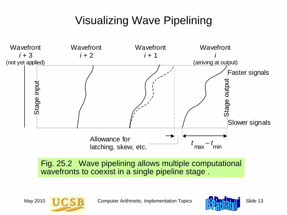
Visualizing Wave PipeliningS
tage
inpu
t
Sta
ge o
utpu
t
Wavefront i + 3
(not yet applied)
Wavefront i + 2
Wavefront i + 1
Wavefront i
(arriving at output)
Faster signals
Slower signals
Allowance for latching, skew, etc. t – t max min
Fig. 25.2 Wave pipelining allows multiple computational wavefronts to coexist in a single pipeline stage .
May 2010 Computer Arithmetic, Implementation Topics Slide 14
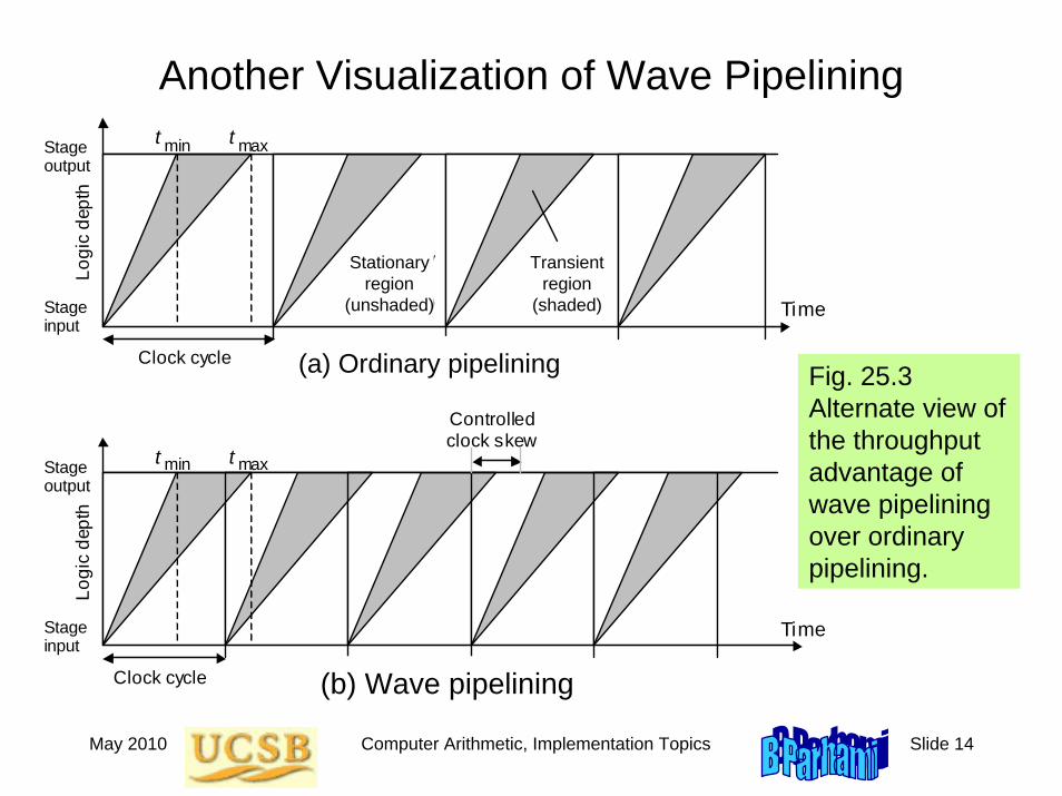
Another Visualization of Wave Pipelining
Fig. 25.3 Alternate view of the throughput advantage of wave pipelining over ordinary pipelining.
Stage output
Stage input
Stationary region
(unshaed)
Transient region
(unshaed)
Clock cycle
Logi
c de
pth
t t min max
Stage output
Stage input
Clock cycle
Logi
c de
pth
t t min max
Time
Time
Controlled clock skew
(a)
(b)
(a) Ordinary pipelining
(b) Wave pipelining
Transientregion
(shaded)
Stationaryregion
(unshaded)
May 2010 Computer Arithmetic, Implementation Topics Slide 15
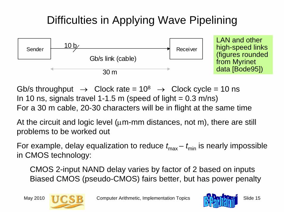
Difficulties in Applying Wave Pipelining
LAN and other high-speed links(figures rounded from Myrinet data [Bode95])
Sender Receiver
Gb/s link (cable)
30 m
10 b
Gb/s throughput → Clock rate = 108 → Clock cycle = 10 nsIn 10 ns, signals travel 1-1.5 m (speed of light = 0.3 m/ns)For a 30 m cable, 20-30 characters will be in flight at the same time
At the circuit and logic level (μm-mm distances, not m), there are still problems to be worked out
For example, delay equalization to reduce tmax – tmin is nearly impossible in CMOS technology:
CMOS 2-input NAND delay varies by factor of 2 based on inputsBiased CMOS (pseudo-CMOS) fairs better, but has power penalty
May 2010 Computer Arithmetic, Implementation Topics Slide 16
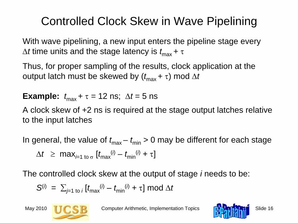
Controlled Clock Skew in Wave PipeliningWith wave pipelining, a new input enters the pipeline stage every Δt time units and the stage latency is tmax + τ
Thus, for proper sampling of the results, clock application at the output latch must be skewed by (tmax + τ) mod Δt
Example: tmax + τ = 12 ns; Δt = 5 ns
A clock skew of +2 ns is required at the stage output latches relative to the input latches
In general, the value of tmax – tmin > 0 may be different for each stage
Δt ≥ maxi=1 to σ [tmax(i) – tmin
(i) + τ]
The controlled clock skew at the output of stage i needs to be:
S(i) = ∑j=1 to i [tmax(i) – tmin
(i) + τ] mod Δt
May 2010 Computer Arithmetic, Implementation Topics Slide 17
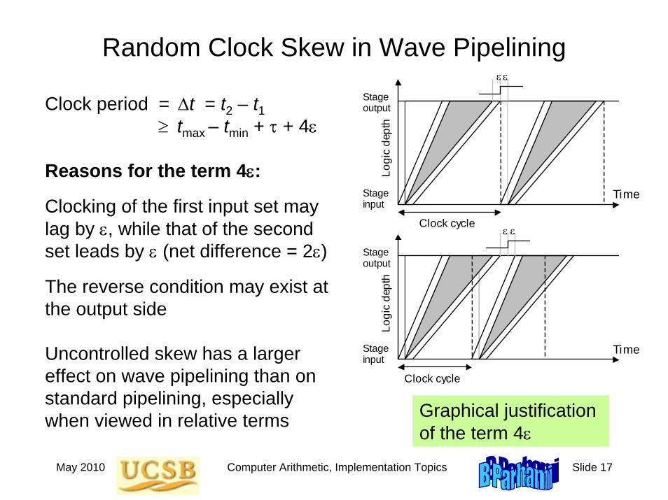
Random Clock Skew in Wave Pipelining
Clock period = Δt = t2 – t1≥ tmax – tmin + τ + 4ε
Reasons for the term 4ε:
Clocking of the first input set may lag by ε, while that of the second set leads by ε (net difference = 2ε)
The reverse condition may exist at the output side
Uncontrolled skew has a larger effect on wave pipelining than on standard pipelining, especially when viewed in relative terms
Stage output
Stage input
Clock cycle
Logi
c de
pth
Stage output
Stage input
Clock cycleLo
gic
dept
h
Time
Time
ε ε
ε ε
Graphical justification of the term 4ε
May 2010 Computer Arithmetic, Implementation Topics Slide 18
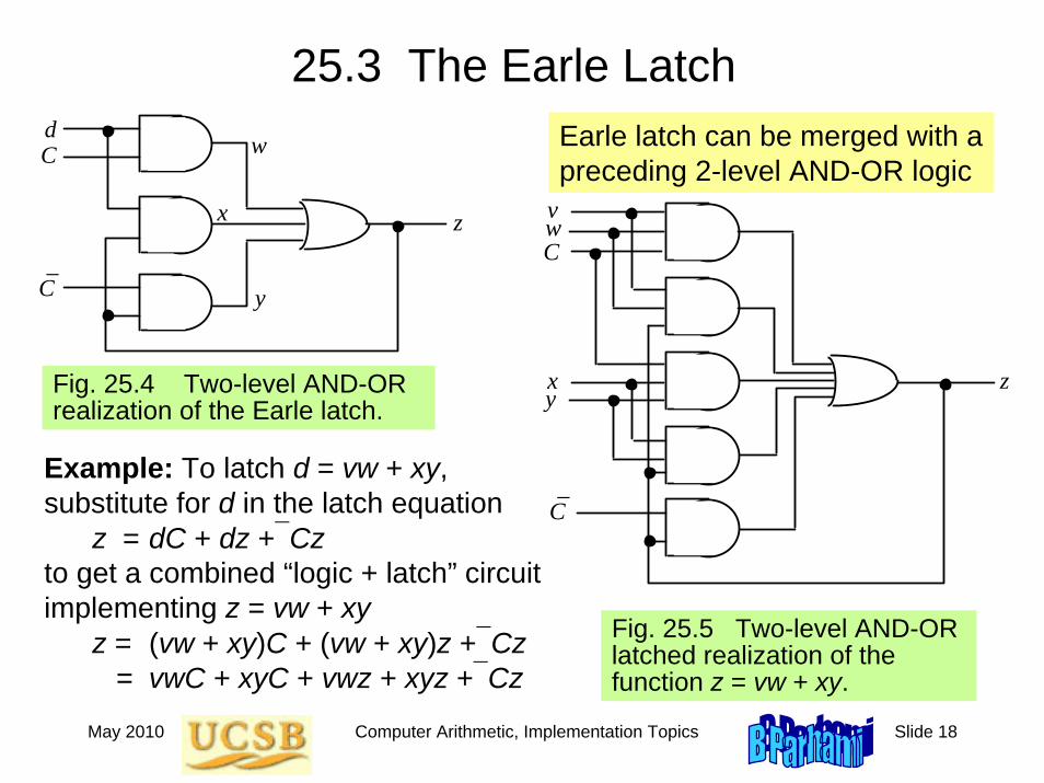
25.3 The Earle Latch
Example: To latch d = vw + xy, substitute for d in the latch equation
z = dC + dz +⎯Czto get a combined “logic + latch” circuit implementing z = vw + xy
z = (vw + xy)C + (vw + xy)z +⎯Cz= vwC + xyC + vwz + xyz +⎯Cz
dC
z
w
x
y_
C
Fig. 25.4 Two-level AND-OR realization of the Earle latch.
C
C
z
vw
xy
_
Fig. 25.5 Two-level AND-OR latched realization of the function z = vw + xy.
Earle latch can be merged with a preceding 2-level AND-OR logic
May 2010 Computer Arithmetic, Implementation Topics Slide 19
Clocking Considerations for Earle Latches
We derived constraints on the maximum clock rate 1/Δt
Clock period Δt has two parts: clock high, and clock low
Δt = Chigh + Clow
Consider a pipeline stage between Earle latches
Chigh must satisfy the inequalities
3δmax – δmin + Smax(C↑,⎯C↓) ≤ Chigh ≤ 2δmin + tmin
δmax and δmin are maximum and minimum gate delays
Smax(C↑,⎯C↓) ≥ 0 is the maximum skew between C↑ and⎯C↓
Clock m ust go low before the fastest signals from the next input data set can affect the input z of the latch
The clock pulse m ust be wide enough to ensure that valid data is stored in the output latch and to avoid logic hazard should C slightly lead C
_
May 2010 Computer Arithmetic, Implementation Topics Slide 20
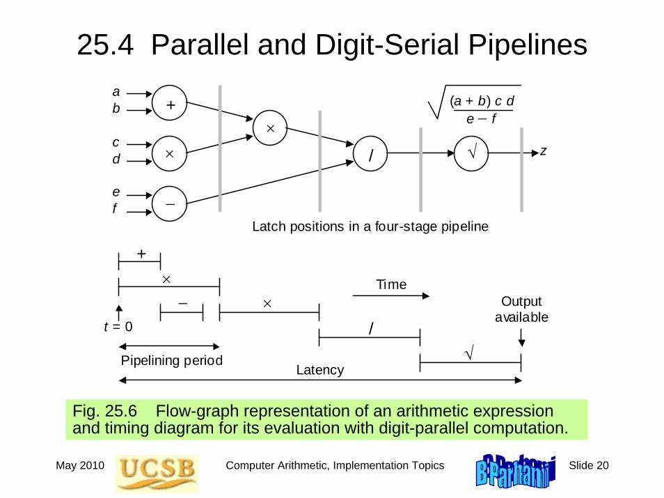
25.4 Parallel and Digit-Serial Pipelines
×
+
×
−
×
/ √
√ /
× −
+
Pipelining period Latency
t = 0
Latch positions in a four-stage pipeline
a b
c d
e f
z
Output available
Time
(a + b) c d e − f
Fig. 25.6 Flow-graph representation of an arithmetic expression and timing diagram for its evaluation with digit-parallel computation.
May 2010 Computer Arithmetic, Implementation Topics Slide 21
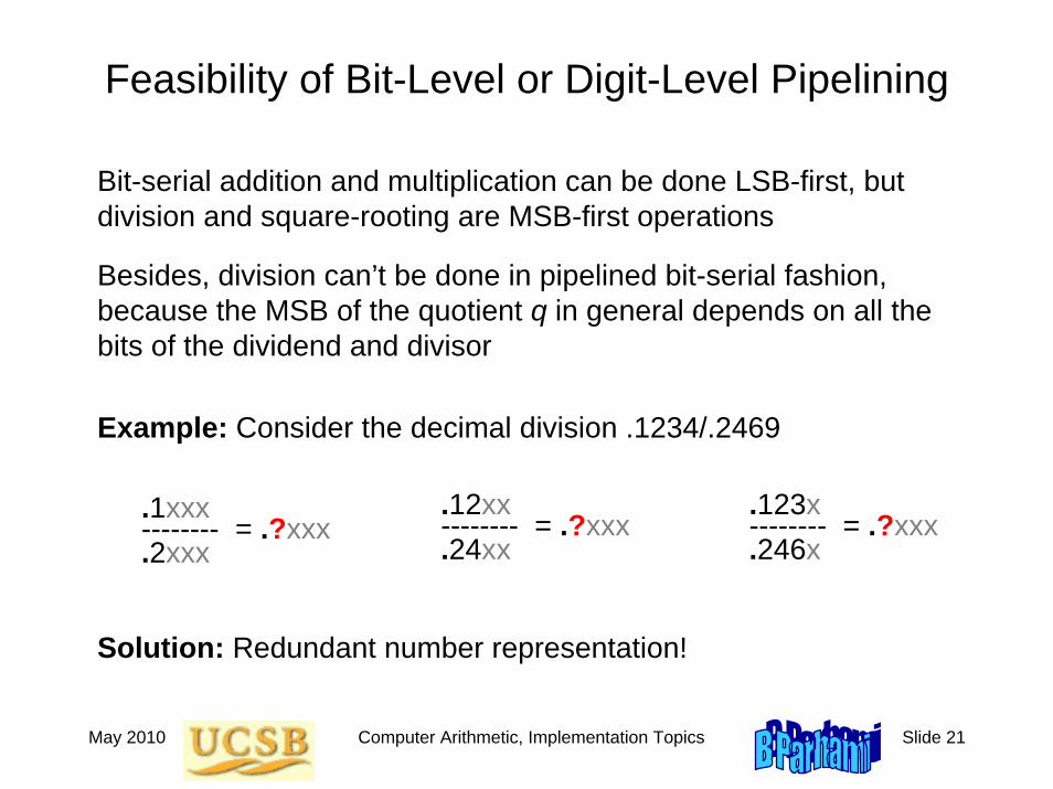
Feasibility of Bit-Level or Digit-Level Pipelining
Bit-serial addition and multiplication can be done LSB-first, but division and square-rooting are MSB-first operations
Besides, division can’t be done in pipelined bit-serial fashion, because the MSB of the quotient q in general depends on all the bits of the dividend and divisor
Example: Consider the decimal division .1234/.2469
Solution: Redundant number representation!
.1xxx-------- = .?xxx.2xxx
.12xx-------- = .?xxx.24xx
.123x-------- = .?xxx.246x
May 2010 Computer Arithmetic, Implementation Topics Slide 22
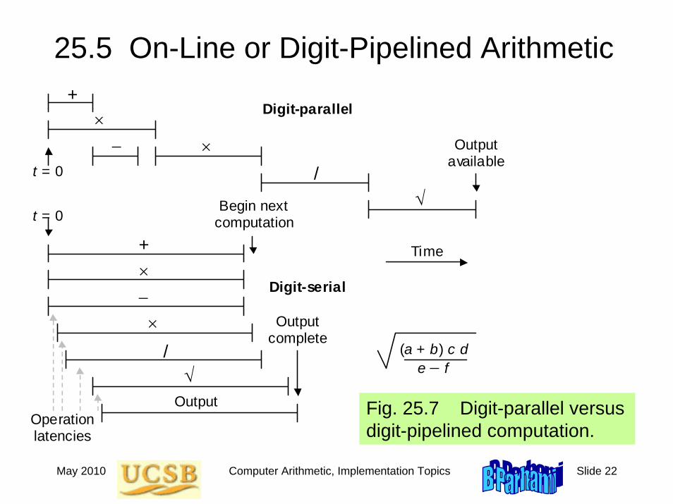
25.5 On-Line or Digit-Pipelined Arithmetic
×
√ /
× −
+
t = 0
Output available
Time
(a + b) c d e − f
×
√ /
× −
+
t = 0
Output complete
Output Operation latencies
Begin next computation
Digit-parallel
Digit-serial
Fig. 25.7 Digit-parallel versus digit-pipelined computation.
May 2010 Computer Arithmetic, Implementation Topics Slide 23
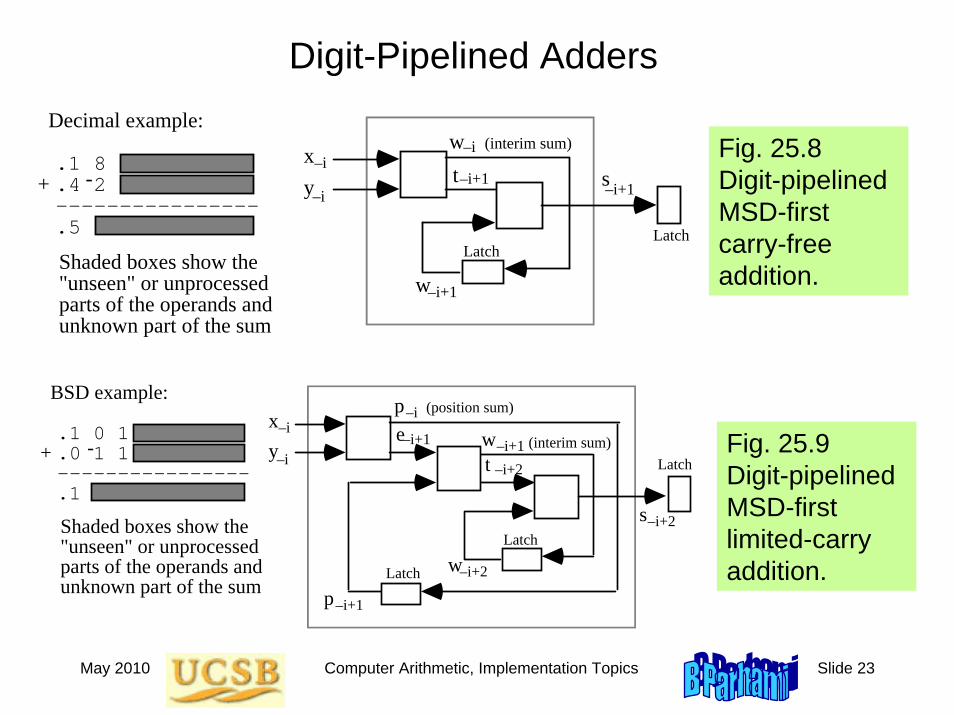
Digit-Pipelined Adders
Fig. 25.8 Digit-pipelined MSD-first carry-free addition.
Decimal example:
.1 8
.4 2 ---------------- .5
Shaded boxes show the "unseen" or unprocessed parts of the operands and unknown part of the sum
+xy t
w
s
w
–i+1
–i+1
–i+1
–i
–i
–i
LatchLatch
(interim sum)
-
Fig. 25.9 Digit-pipelined MSD-first limited-carry addition.
BSD example:
.1 0 1
.0 1 1 ---------------- .1
Shaded boxes show the "unseen" or unprocessed parts of the operands and unknown part of the sum
+xy
ep
s
p
–i+2
–i+1
–i+1
–i
–i
–i
Latch
Latch
(position sum)
w–i+1 (interim sum)
w–i+2
Latch
t –i+2-
May 2010 Computer Arithmetic, Implementation Topics Slide 24
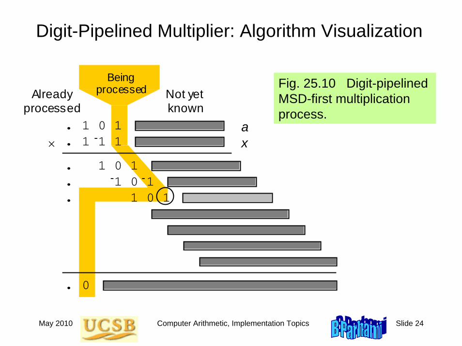
Digit-Pipelined Multiplier: Algorithm Visualization
Fig. 25.10 Digit-pipelined MSD-first multiplication process.
. 1 0 1
. 1 1 1
. 1 0 1
. 1 0 1
. 1 0 1
-
- -
. 0
a x
Already processed
Being processed Not yet
known
×
May 2010 Computer Arithmetic, Implementation Topics Slide 25
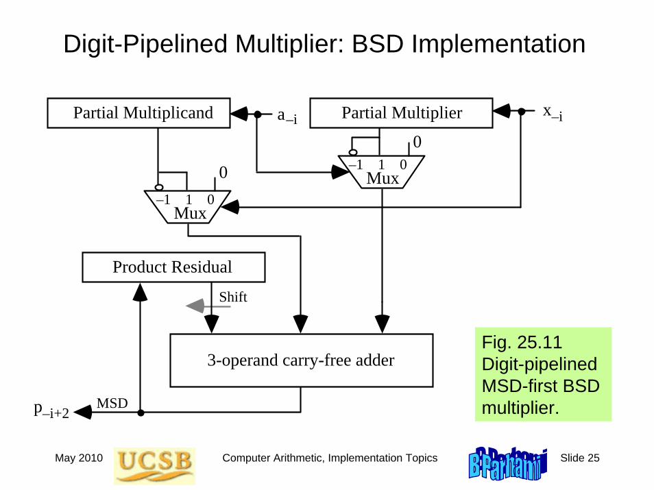
Digit-Pipelined Multiplier: BSD Implementation
Fig. 25.11 Digit-pipelined MSD-first BSD multiplier.
a
Mux–1 1 0
0
x
Mux
0
p
3-operand carry-free adder
Partial Multiplicand Partial Multiplier
Product Residual
Shift
–i+2
–i–i
–1 1 0
MSD
May 2010 Computer Arithmetic, Implementation Topics Slide 26
Digit-Pipelined Divider
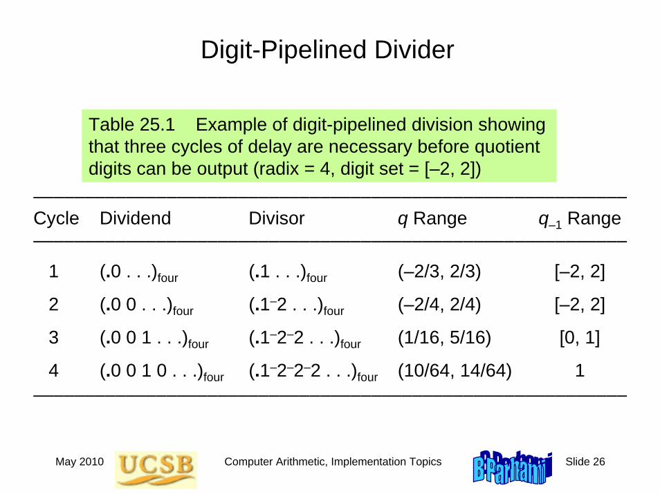
Table 25.1 Example of digit-pipelined division showing that three cycles of delay are necessary before quotient digits can be output (radix = 4, digit set = [–2, 2])
––––––––––––––––––––––––––––––––––––––––––––––––––––––––––Cycle Dividend Divisor q Range q–1 Range––––––––––––––––––––––––––––––––––––––––––––––––––––––––––
1 (.0 . . .)four (.1 . . .)four (–2/3, 2/3) [–2, 2]
2 (.0 0 . . .)four (.1–2 . . .)four (–2/4, 2/4) [–2, 2]
3 (.0 0 1 . . .)four (.1–2–2 . . .)four (1/16, 5/16) [0, 1]
4 (.0 0 1 0 . . .)four (.1–2–2–2 . . .)four (10/64, 14/64) 1––––––––––––––––––––––––––––––––––––––––––––––––––––––––––
May 2010 Computer Arithmetic, Implementation Topics Slide 27
Digit-Pipelined Square-Rooter
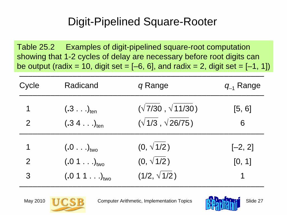
Table 25.2 Examples of digit-pipelined square-root computation showing that 1-2 cycles of delay are necessary before root digits can be output (radix = 10, digit set = [–6, 6], and radix = 2, digit set = [–1, 1])–––––––––––––––––––––––––––––––––––––––––––––––––––––––Cycle Radicand q Range q–1 Range–––––––––––––––––––––––––––––––––––––––––––––––––––––––
1 (.3 . . .)ten (√ 7/30 , √ 11/30 ) [5, 6]
2 (.3 4 . . .)ten (√ 1/3 , √ 26/75 ) 6–––––––––––––––––––––––––––––––––––––––––––––––––––––––
1 (.0 . . .)two (0, √ 1/2 ) [–2, 2]
2 (.0 1 . . .)two (0, √ 1/2 ) [0, 1]
3 (.0 1 1 . . .)two (1/2, √ 1/2 ) 1–––––––––––––––––––––––––––––––––––––––––––––––––––––––
May 2010 Computer Arithmetic, Implementation Topics Slide 28
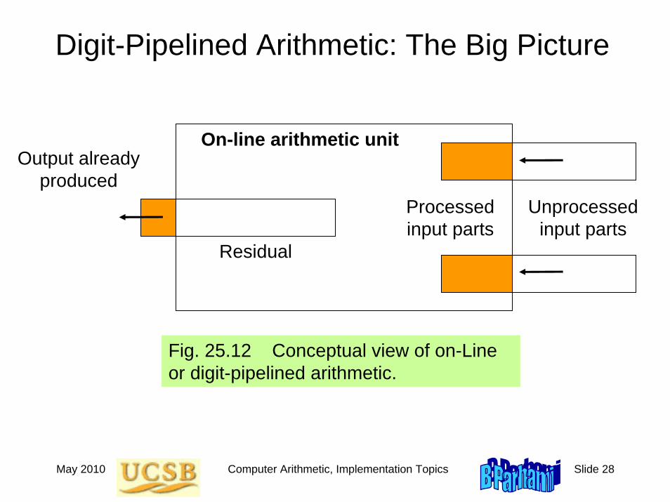
Digit-Pipelined Arithmetic: The Big Picture
Fig. 25.12 Conceptual view of on-Line or digit-pipelined arithmetic.
Output already produced
Residual
Processed input parts
Unprocessed input parts
On-line arithmetic unit
May 2010 Computer Arithmetic, Implementation Topics Slide 29
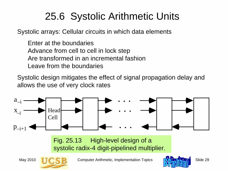
25.6 Systolic Arithmetic UnitsSystolic arrays: Cellular circuits in which data elements
Enter at the boundariesAdvance from cell to cell in lock stepAre transformed in an incremental fashionLeave from the boundaries
Systolic design mitigates the effect of signal propagation delay and allows the use of very clock rates
Fig. 25.13 High-level design of a systolic radix-4 digit-pipelined multiplier.
ax–i
–i . . .. . .. . .p–i+1
Head Cell
May 2010 Computer Arithmetic, Implementation Topics Slide 30
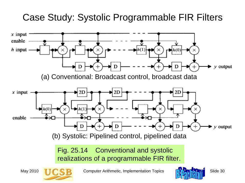
Case Study: Systolic Programmable FIR Filters
Fig. 25.14 Conventional and systolic realizations of a programmable FIR filter.
(a) Conventional: Broadcast control, broadcast data
(b) Systolic: Pipelined control, pipelined data
May 2010 Computer Arithmetic, Implementation Topics Slide 31
26 Low-Power Arithmetic
Chapter GoalsLearn how to improve the power efficiencyof arithmetic circuits by means ofalgorithmic and logic design strategies
Chapter HighlightsReduced power dissipation needed due to
• Limited source (portable, embedded)• Difficulty of heat disposal
Algorithm and logic-level methods: discussedTechnology and circuit methods: ignored here
May 2010 Computer Arithmetic, Implementation Topics Slide 32
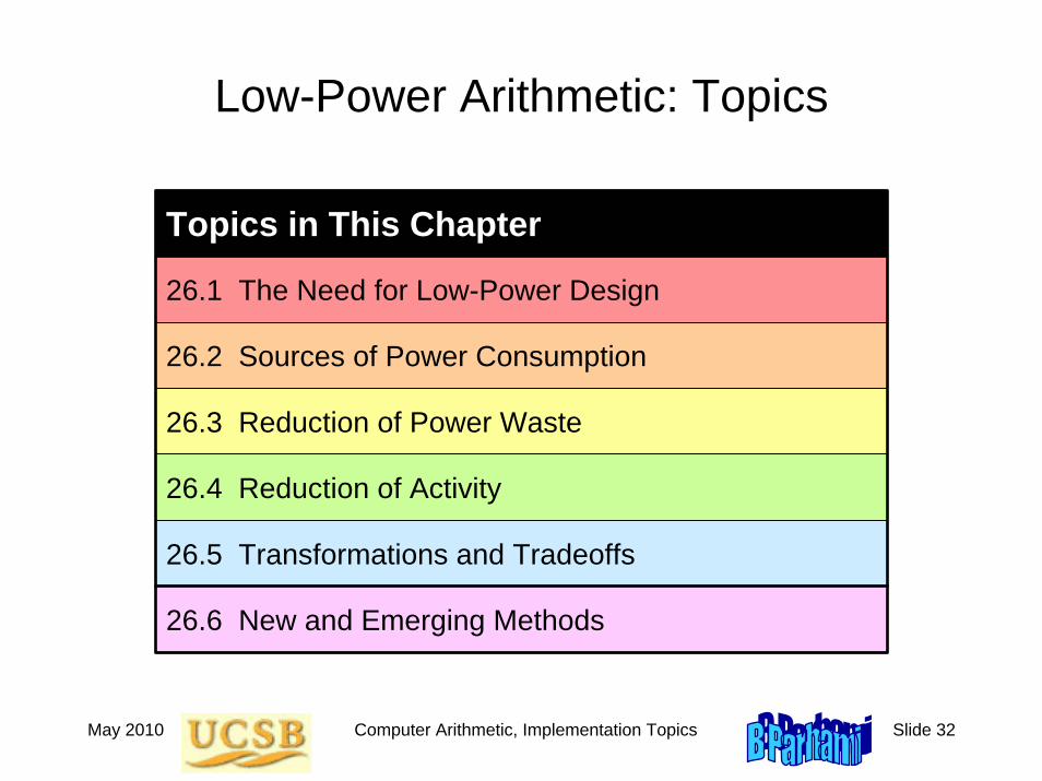
Low-Power Arithmetic: Topics
Topics in This Chapter
26.1 The Need for Low-Power Design
26.2 Sources of Power Consumption
26.3 Reduction of Power Waste
26.4 Reduction of Activity
26.5 Transformations and Tradeoffs
26.6 New and Emerging Methods
May 2010 Computer Arithmetic, Implementation Topics Slide 33
26.1 The Need for Low-Power Design
-
Portable and wearable electronic devices
Lithium-ion batteries: 0.2 watt-hr per gram of weight
Practical battery weight < 500 g (< 50 g if wearable device)
Total power ≅ 5-10 watt for a day’s work between recharges
Modern high-performance microprocessors use 100s watts
Power is proportional to die area × clock frequency
Cooling of micros difficult, but still manageable
Cooling of MPPs and server farms is a BIG challenge
New battery technologies cannot keep pace with demand
Demand for more speed and functionality (multimedia, etc.)
May 2010 Computer Arithmetic, Implementation Topics Slide 34
Processor Power Consumption Trends
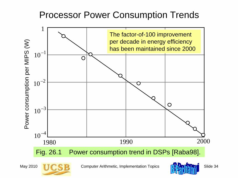
Fig. 26.1 Power consumption trend in DSPs [Raba98].1980 1990 2000
10–4
10–3
10–2
10–1
1P
ower
con
sum
ptio
n pe
r MIP
S (W
)The factor-of-100 improvement per decade in energy efficiency has been maintained since 2000
May 2010 Computer Arithmetic, Implementation Topics Slide 35
26.2 Sources of Power Consumption
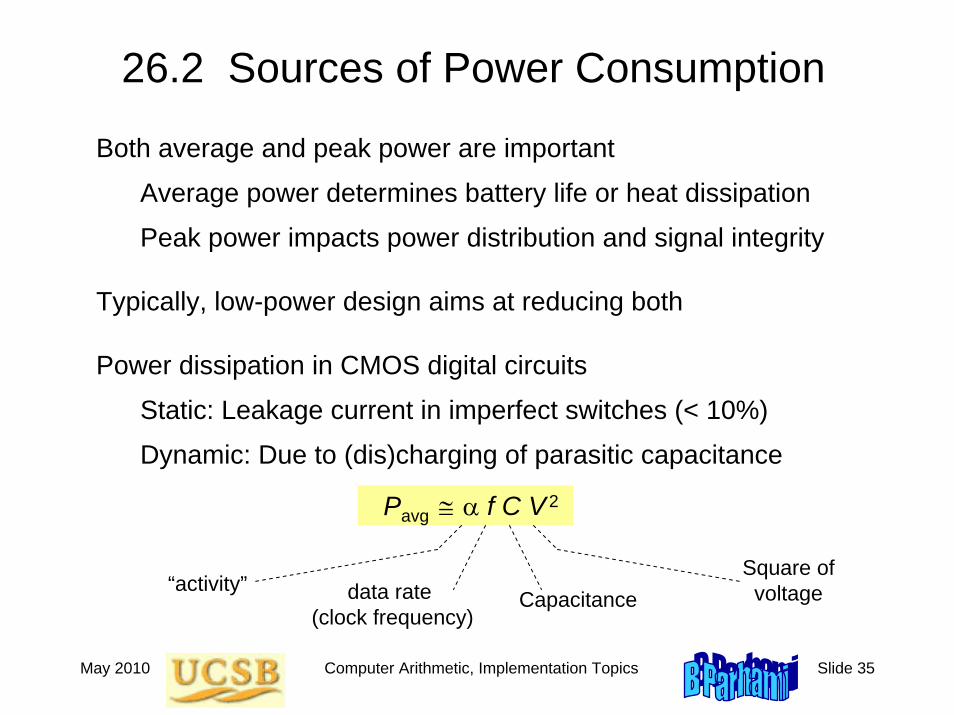
Both average and peak power are important
Average power determines battery life or heat dissipation
Peak power impacts power distribution and signal integrity
Typically, low-power design aims at reducing both
Power dissipation in CMOS digital circuits
Static: Leakage current in imperfect switches (< 10%)
Dynamic: Due to (dis)charging of parasitic capacitance
Pavg ≅ α f C V 2
data rate (clock frequency)
CapacitanceSquare of voltage“activity”
May 2010 Computer Arithmetic, Implementation Topics Slide 36
Power Reduction Strategies: The Big Picture
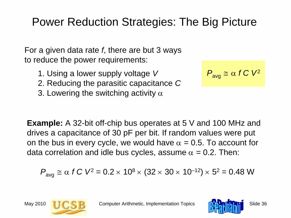
Pavg ≅ α f C V 2
For a given data rate f, there are but 3 ways to reduce the power requirements:
1. Using a lower supply voltage V2. Reducing the parasitic capacitance C3. Lowering the switching activity α
Example: A 32-bit off-chip bus operates at 5 V and 100 MHz and drives a capacitance of 30 pF per bit. If random values were puton the bus in every cycle, we would have α = 0.5. To account for data correlation and idle bus cycles, assume α = 0.2. Then:
Pavg ≅ α f C V 2 = 0.2 × 108 × (32 × 30 × 10–12) × 52 = 0.48 W
May 2010 Computer Arithmetic, Implementation Topics Slide 37
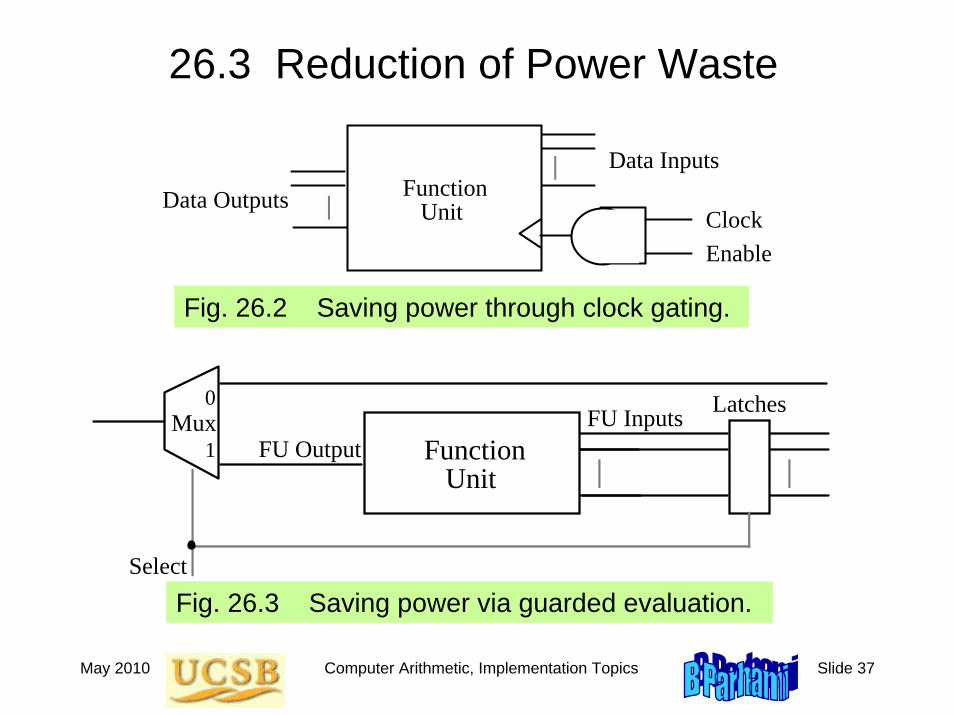
26.3 Reduction of Power Waste
Function Unit Clock
Enable
Data Inputs
Data Outputs
Function Unit
FU InputsFU Output
Mux
Select
Latches0 1
Fig. 26.3 Saving power via guarded evaluation.
Fig. 26.2 Saving power through clock gating.
May 2010 Computer Arithmetic, Implementation Topics Slide 38
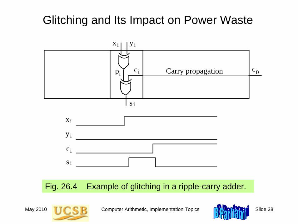
Glitching and Its Impact on Power Waste
s i
xi yi
ci c0Carry propagationpi
xi
yi
s i
ci
Fig. 26.4 Example of glitching in a ripple-carry adder.
May 2010 Computer Arithmetic, Implementation Topics Slide 39
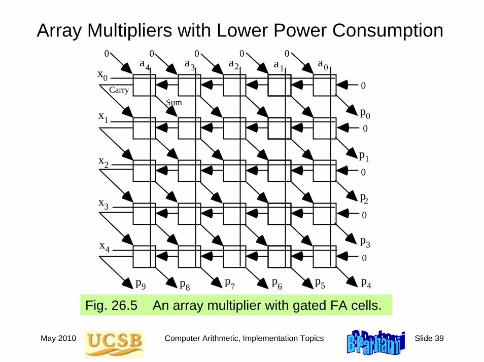
Array Multipliers with Lower Power Consumption
p0
p1
p2
p3
p4p6p7p8
0 0 0
p9 p5
0 0
0
0
0
0
0
a0a1a2a3a4
x4
x3
x2
x1
x0Carry
Sum
Fig. 26.5 An array multiplier with gated FA cells.
May 2010 Computer Arithmetic, Implementation Topics Slide 40
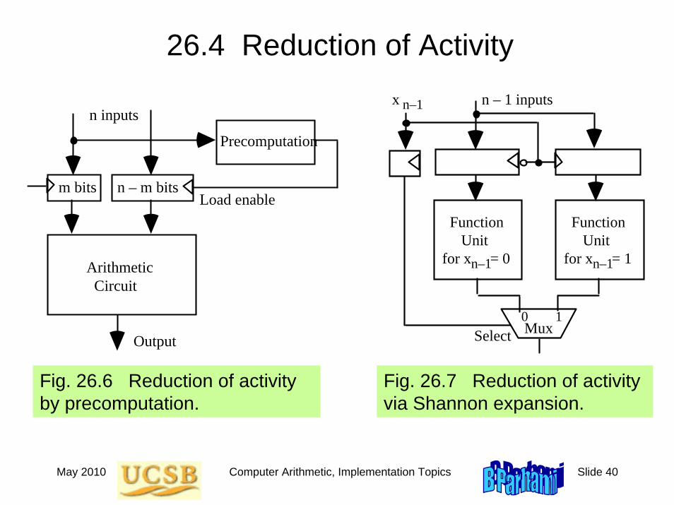
26.4 Reduction of Activity
Fig. 26.6 Reduction of activity by precomputation.
Arithmetic Circuit
m bits n – m bits
Precomputation
n inputs
Output
Load enable
n – 1 inputs
Function Unit for x = 0
Function Unit for x = 1
Select
x n–1
Mux 0 1
n–1n–1
Fig. 26.7 Reduction of activity via Shannon expansion.
May 2010 Computer Arithmetic, Implementation Topics Slide 41
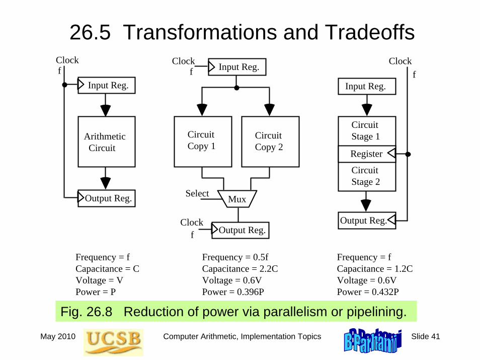
26.5 Transformations and Tradeoffs
Fig. 26.8 Reduction of power via parallelism or pipelining.
Clock
Arithmetic Circuit
f
Frequency = f Capacitance = C Voltage = V Power = P
Frequency = 0.5f Capacitance = 2.2C Voltage = 0.6V Power = 0.396P
Frequency = f Capacitance = 1.2C Voltage = 0.6V Power = 0.432P
Circuit Copy 1
Circuit Copy 2
Mux
Circuit Stage 1
Circuit Stage 2
Clockf
Register
Input Reg. Input Reg.
Output Reg.
Output Reg.Clock
f
Select
Input Reg.Clockf
Output Reg.
May 2010 Computer Arithmetic, Implementation Topics Slide 42
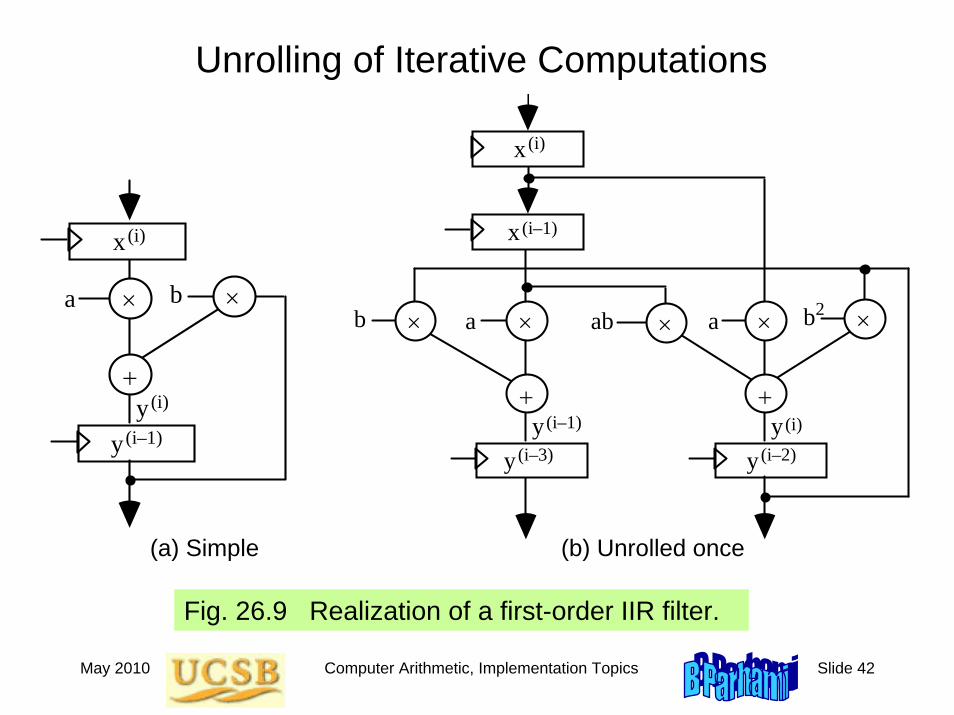
Unrolling of Iterative Computations
Fig. 26.9 Realization of a first-order IIR filter.
x(i)
×
+
×a b
y(i–1)y(i)
x
×
+
× ab
y (i)
×
+
×a b
yy(i–2)
2×ab
y(i–3)
x
(i–1)
(i)
(i–1)
(a) Simple (b) Unrolled once
May 2010 Computer Arithmetic, Implementation Topics Slide 43
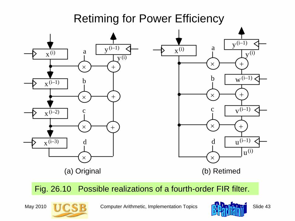
Retiming for Power Efficiency
Fig. 26.10 Possible realizations of a fourth-order FIR filter.
x (i) a
x (i–1)
x (i–3)
b
d
×
×
×
+
+
y (i)y (i–1)
x (i–2) c
×
+
x(i) a
b
d
×
×
×
+
+
y(i)y (i–1)
c
×
+
u(i)
v (i–1)
w (i–1)
u(i–1)
(a) Original (b) Retimed
May 2010 Computer Arithmetic, Implementation Topics Slide 44
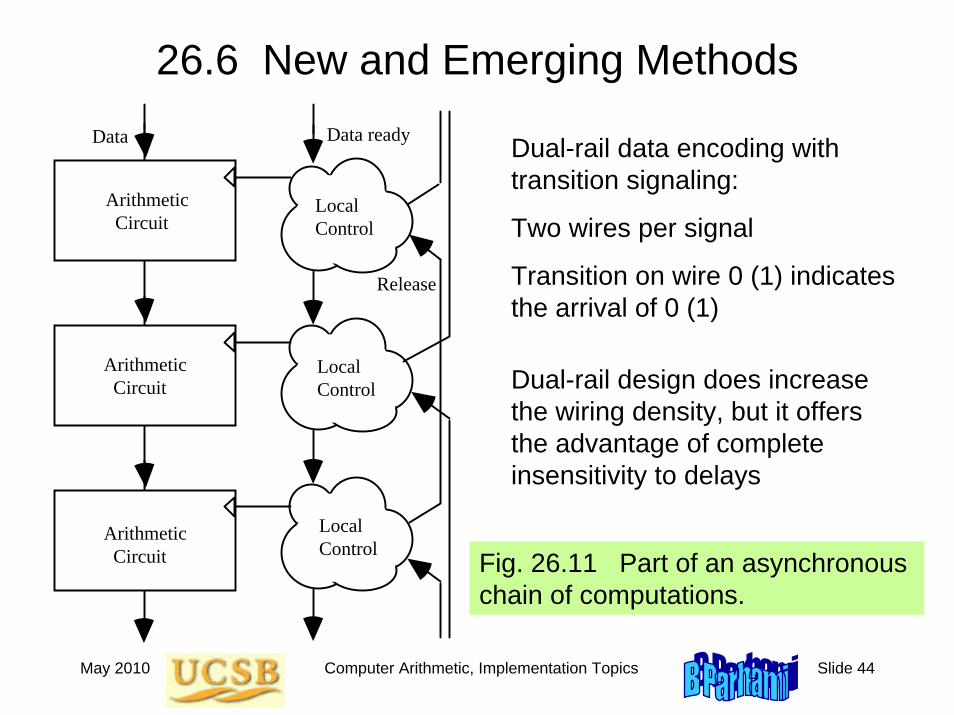
26.6 New and Emerging Methods
Local Control
Local Control
Local Control
Arithmetic Circuit
Arithmetic Circuit
Arithmetic Circuit
Data readyData
Release
Fig. 26.11 Part of an asynchronous chain of computations.
Dual-rail data encoding with transition signaling:
Two wires per signal
Transition on wire 0 (1) indicates the arrival of 0 (1)
Dual-rail design does increase the wiring density, but it offers the advantage of complete insensitivity to delays
May 2010 Computer Arithmetic, Implementation Topics Slide 45
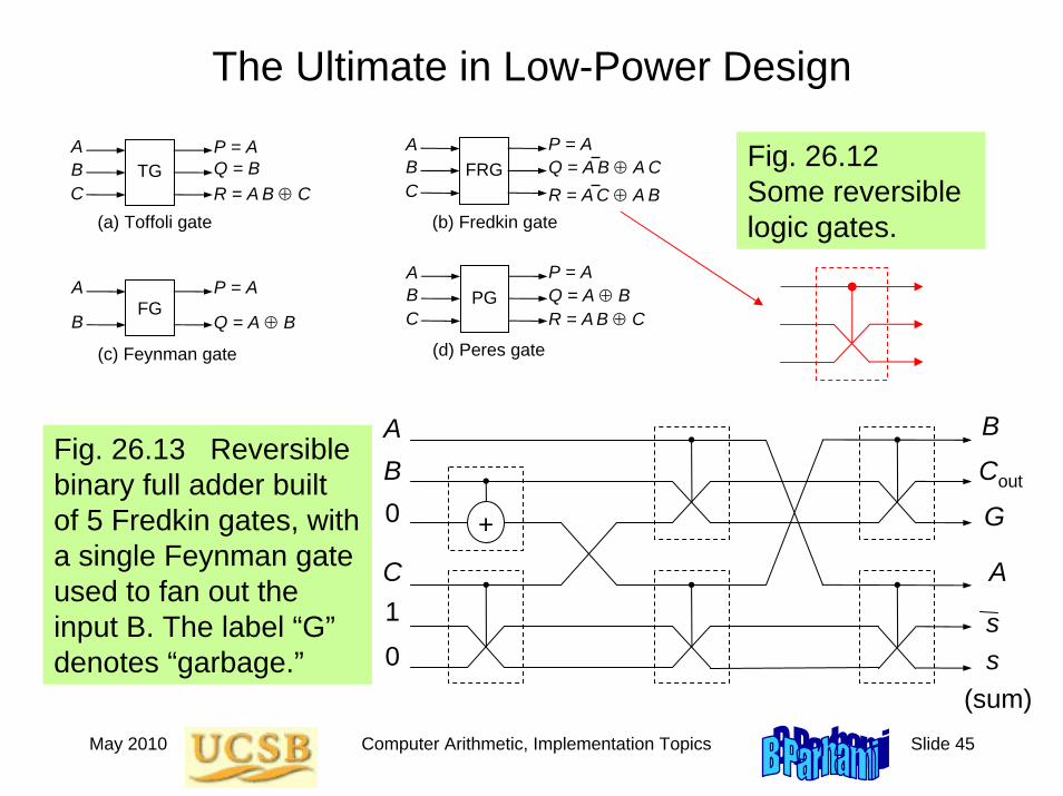
The Ultimate in Low-Power Design
Fig. 26.12 Some reversible logic gates.
ABC
P = AQ = BR = A B ⊕ C
TG
(a) Toffoli gate
ABC
FRG
(b) Fredkin gate
A
B
P = A
Q = A ⊕ BFG
(c) Feynman gate
ABC
P = A
R = A B ⊕ CPG Q = A ⊕ B
(d) Peres gate
P = A
R = A C ⊕ A BQ = A B ⊕ A C
B0
C1
0
+
ACout
s(sum)
B
A
G
s
Fig. 26.13 Reversible binary full adder built of 5 Fredkin gates, with a single Feynman gate used to fan out the input B. The label “G”denotes “garbage.”
May 2010 Computer Arithmetic, Implementation Topics Slide 46
27 Fault-Tolerant ArithmeticChapter Goals
Learn about errors due to hardware faultsor hostile environmental conditions,and how to deal with or circumvent them
Chapter HighlightsModern components are very robust, but . . .
put millions /billions of them togetherand something is bound to go wrong
Can arithmetic be protected via encoding?Reliable circuits and robust algorithms
May 2010 Computer Arithmetic, Implementation Topics Slide 47
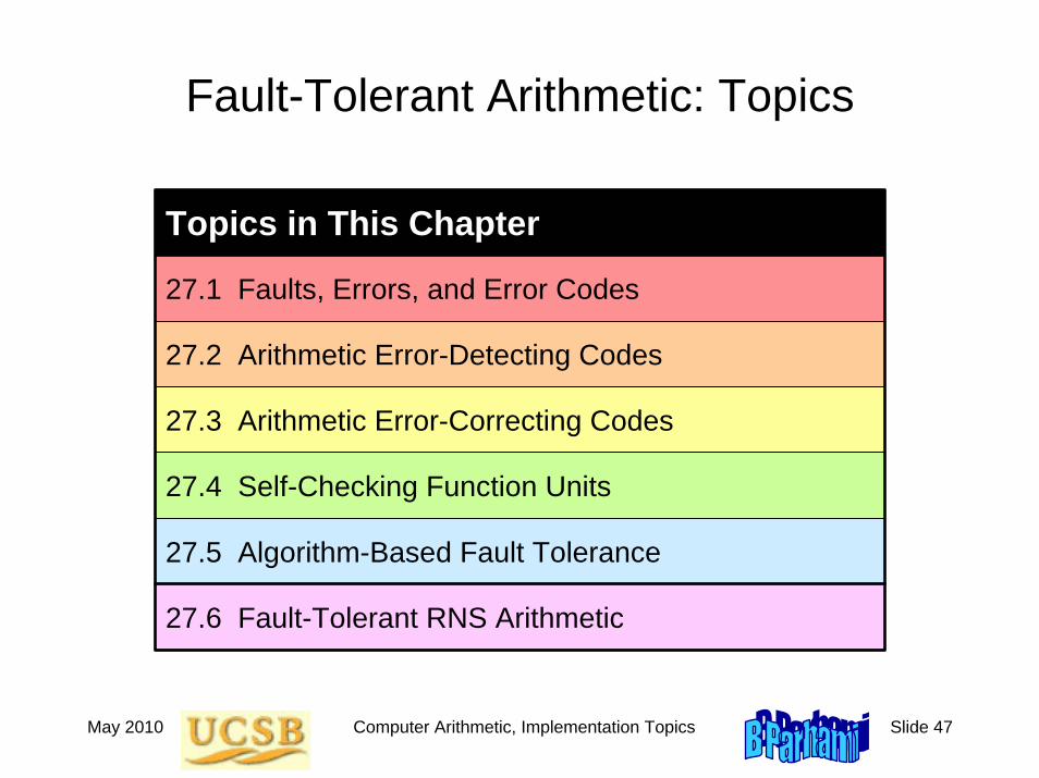
Fault-Tolerant Arithmetic: Topics
Topics in This Chapter
27.1 Faults, Errors, and Error Codes
27.2 Arithmetic Error-Detecting Codes
27.3 Arithmetic Error-Correcting Codes
27.4 Self-Checking Function Units
27.5 Algorithm-Based Fault Tolerance
27.6 Fault-Tolerant RNS Arithmetic
May 2010 Computer Arithmetic, Implementation Topics Slide 48
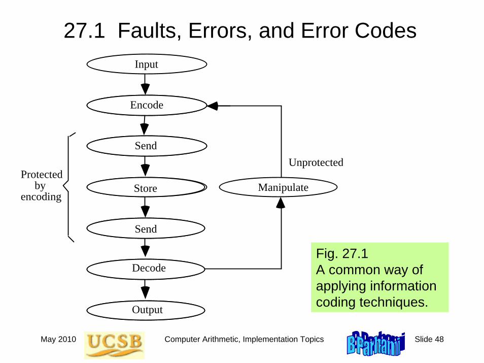
27.1 Faults, Errors, and Error Codes
Protected by Encoding
Input
Encode
Send
Store
Send
Decode
Output
Manipulate
Unprotected Protected
by encoding
Fig. 27.1 A common way of applying information coding techniques.
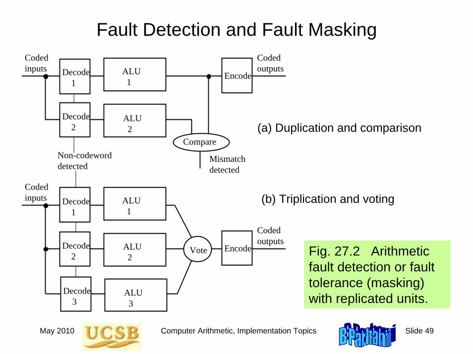
May 2010 Computer Arithmetic, Implementation Topics Slide 49
Fault Detection and Fault MaskingCoded inputs Decode
1
Decode 2
ALU 1
ALU 2
Compare
Mismatch detected
Encode
Coded outputs
Coded inputs Decode
1
Decode 2
ALU 1
ALU 2
Decode 3
ALU 3
Vote Encode
Coded outputs
Non-codeword detected
Fig. 27.2 Arithmetic fault detection or fault tolerance (masking) with replicated units.
(a) Duplication and comparison
(b) Triplication and voting
May 2010 Computer Arithmetic, Implementation Topics Slide 50
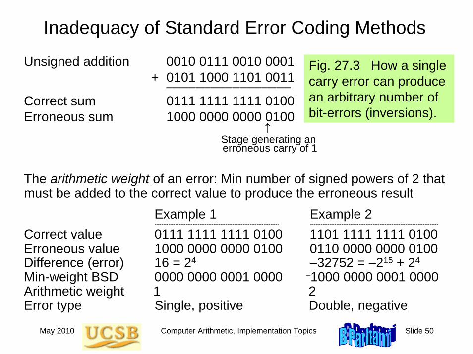
Inadequacy of Standard Error Coding Methods
Unsigned addition 0010 0111 0010 0001+ 0101 1000 1101 0011
–––––––––––––––––Correct sum 0111 1111 1111 0100Erroneous sum 1000 0000 0000 0100
↑Stage generating anerroneous carry of 1
Fig. 27.3 How a single carry error can produce an arbitrary number of bit-errors (inversions).
The arithmetic weight of an error: Min number of signed powers of 2 that must be added to the correct value to produce the erroneous result
Example 1 Example 2------------------------------------------------------------------------ --------------------------------------------------------------------------
Correct value 0111 1111 1111 0100 1101 1111 1111 0100Erroneous value 1000 0000 0000 0100 0110 0000 0000 0100Difference (error) 16 = 24 –32752 = –215 + 24
Min-weight BSD 0000 0000 0001 0000 –1000 0000 0001 0000Arithmetic weight 1 2Error type Single, positive Double, negative
May 2010 Computer Arithmetic, Implementation Topics Slide 51
27.2 Arithmetic Error-Detecting Codes
Arithmetic error-detecting codes:
Are characterized by arithmetic weights of detectable errors
Allow direct arithmetic on coded operands
We will discuss two classes of arithmetic error-detecting codes, both of which are based on a check modulus A (usually a small odd number)
Product or AN codesRepresent the value N by the number AN
Residue (or inverse residue) codesRepresent the value N by the pair (N, C),where C is N mod A or (N – N mod A) mod A
May 2010 Computer Arithmetic, Implementation Topics Slide 52
Product or AN Codes
For odd A, all weight-1 arithmetic errors are detected
Arithmetic errors of weight ≥ 2 may go undetected
e.g., the error 32 736 = 215 – 25 undetectable with A = 3, 11, or 31
Error detection: check divisibility by A
Encoding/decoding: multiply/divide by A
Arithmetic also requires multiplication and division by A
Product codes are nonseparate (nonseparable) codesData and redundant check info are intermixed
May 2010 Computer Arithmetic, Implementation Topics Slide 53
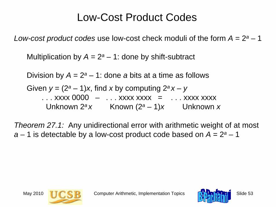
Low-Cost Product Codes
Low-cost product codes use low-cost check moduli of the form A = 2a – 1
Multiplication by A = 2a – 1: done by shift-subtract
Division by A = 2a – 1: done a bits at a time as follows
Given y = (2a – 1)x, find x by computing 2a x – y. . . xxxx 0000 – . . . xxxx xxxx = . . . xxxx xxxxUnknown 2a x Known (2a – 1)x Unknown x
Theorem 27.1: Any unidirectional error with arithmetic weight of at most a – 1 is detectable by a low-cost product code based on A = 2a – 1
May 2010 Computer Arithmetic, Implementation Topics Slide 54
Arithmetic on AN-Coded Operands
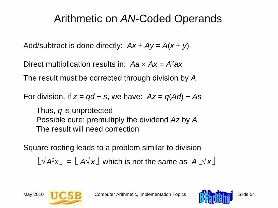
Add/subtract is done directly: Ax ± Ay = A(x ± y)
Direct multiplication results in: Aa × Ax = A2ax
The result must be corrected through division by A
For division, if z = qd + s, we have: Az = q(Ad) + As
Thus, q is unprotectedPossible cure: premultiply the dividend Az by AThe result will need correction
Square rooting leads to a problem similar to division
⎣√ A2x ⎦ = ⎣ A√ x ⎦ which is not the same as A ⎣√ x ⎦
May 2010 Computer Arithmetic, Implementation Topics Slide 55
Residue and Inverse Residue Codes
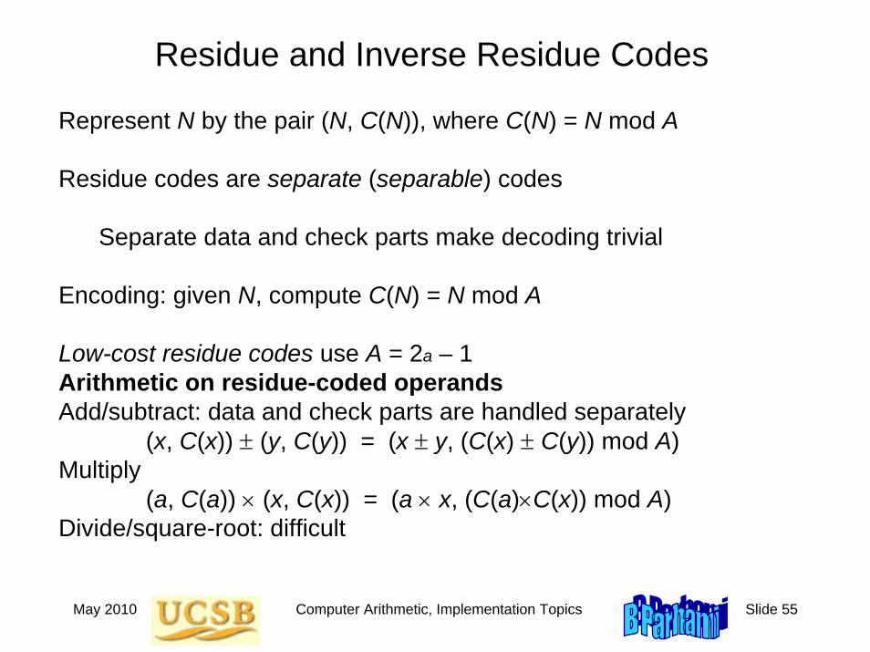
Represent N by the pair (N, C(N)), where C(N) = N mod A
Residue codes are separate (separable) codes
Separate data and check parts make decoding trivial
Encoding: given N, compute C(N) = N mod A
Low-cost residue codes use A = 2a – 1Arithmetic on residue-coded operandsAdd/subtract: data and check parts are handled separately
(x, C(x)) ± (y, C(y)) = (x ± y, (C(x) ± C(y)) mod A)Multiply
(a, C(a)) × (x, C(x)) = (a × x, (C(a)×C(x)) mod A)Divide/square-root: difficult
May 2010 Computer Arithmetic, Implementation Topics Slide 56
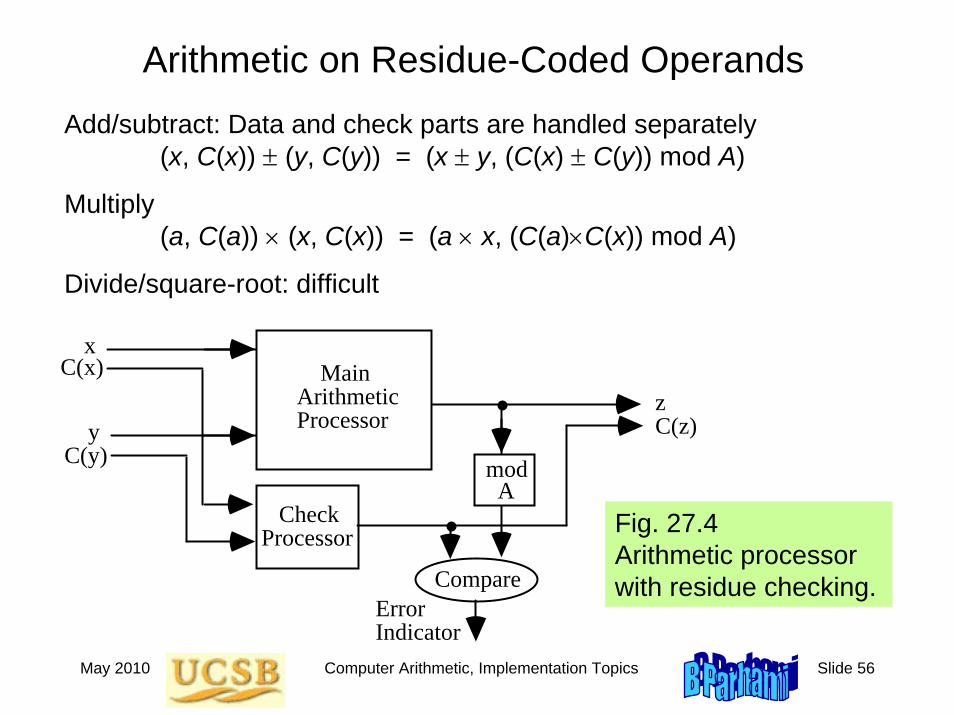
Arithmetic on Residue-Coded OperandsAdd/subtract: Data and check parts are handled separately
(x, C(x)) ± (y, C(y)) = (x ± y, (C(x) ± C(y)) mod A)
Multiply (a, C(a)) × (x, C(x)) = (a × x, (C(a)×C(x)) mod A)
Divide/square-root: difficult
Main Arithmetic Processor
Check Processor
x
y
C(x)
C(y)
z
Compare
mod
C(z)
Error Indicator
AFig. 27.4 Arithmetic processor with residue checking.
May 2010 Computer Arithmetic, Implementation Topics Slide 57
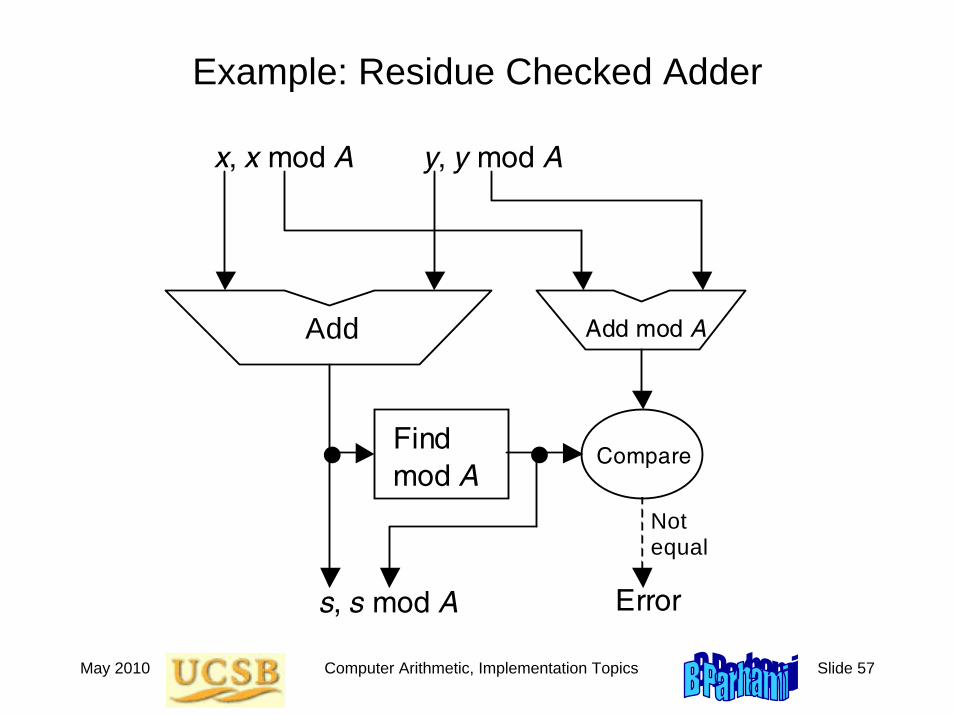
Example: Residue Checked Adder
Add
x, x mod A
Add mod A
Compare Find mod A
y, y mod A
s, s mod A Error
Not equal
May 2010 Computer Arithmetic, Implementation Topics Slide 58
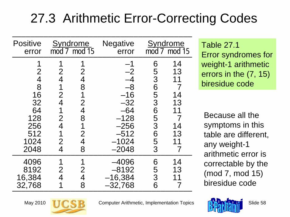
27.3 Arithmetic Error-Correcting Codes––––––––––––––––––––––––––––––––––––––––Positive Syndrome Negative Syndrome
error mod 7 mod 15 error mod 7 mod 15––––––––––––––––––––––––––––––––––––––––
1 1 1 –1 6 142 2 2 –2 5 134 4 4 –4 3 118 1 8 –8 6 7
16 2 1 –16 5 1432 4 2 –32 3 1364 1 4 –64 6 11
128 2 8 –128 5 7256 4 1 –256 3 14512 1 2 –512 6 13
1024 2 4 –1024 5 112048 4 8 –2048 3 7
––––––––––––––––––––––––––––––––––––––––4096 1 1 –4096 6 148192 2 2 –8192 5 13
16,384 4 4 –16,384 3 1132,768 1 8 –32,768 6 7
––––––––––––––––––––––––––––––––––––––––
Table 27.1 Error syndromes for weight-1 arithmetic errors in the (7, 15) biresidue code
Because all the symptoms in this table are different, any weight-1 arithmetic error is correctable by the (mod 7, mod 15) biresidue code
May 2010 Computer Arithmetic, Implementation Topics Slide 59
Properties of Biresidue Codes
Biresidue code with relatively prime low-cost check moduli A = 2a – 1 and B = 2b – 1 supports a × b bits of data for weight-1 error correction
Representational redundancy = (a + b)/(ab) = 1/a + 1/b
May 2010 Computer Arithmetic, Implementation Topics Slide 60
27.4 Self-Checking Function Units
Self-checking (SC) unit: any fault from a prescribed set does not affect the correct output (masked) or leads to a noncodewordoutput (detected)
An invalid result is:
Detected immediately by a code checker, or
Propagated downstream by the next self-checking unit
To build SC units, we need SC code checkers that never validate a noncodeword, even when they are faulty
May 2010 Computer Arithmetic, Implementation Topics Slide 61
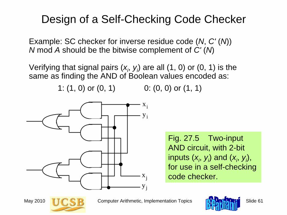
Design of a Self-Checking Code Checker
Example: SC checker for inverse residue code (N, C' (N)) N mod A should be the bitwise complement of C' (N)
Verifying that signal pairs (xi, yi) are all (1, 0) or (0, 1) is the same as finding the AND of Boolean values encoded as:
1: (1, 0) or (0, 1) 0: (0, 0) or (1, 1)
xyi
i
xyj
j
Fig. 27.5 Two-input AND circuit, with 2-bit inputs (xi, yi) and (xi, yi), for use in a self-checking code checker.
May 2010 Computer Arithmetic, Implementation Topics Slide 62
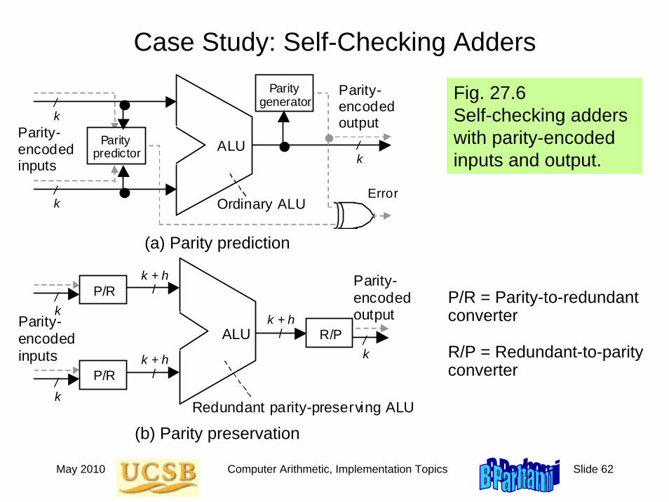
Case Study: Self-Checking Adders
P/R = Parity-to-redundant converter
R/P = Redundant-to-parity converter
Fig. 27.6 Self-checking adders with parity-encoded inputs and output.
/ k
/ k
/ k
Parity- encoded inputs
ALU
Error
Parity- encoded output
Parity generator
Ordinary ALU
(b) Parity prediction
Parity predictor
/ k
Parity- encoded inputs
ALU
k + h / P/R
k + h /
/ k
Parity- encoded output
R/P
/ k
P/R
k + h /
Redundant parity-preserving ALU
(c) Parity/redundant and redundant/parity code conversion
(a) Parity prediction
(b) Parity preservation
May 2010 Computer Arithmetic, Implementation Topics Slide 63
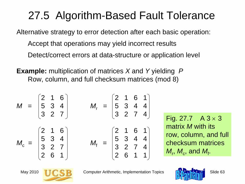
27.5 Algorithm-Based Fault ToleranceAlternative strategy to error detection after each basic operation:
Accept that operations may yield incorrect results
Detect/correct errors at data-structure or application level
Fig. 27.7 A 3 × 3 matrix M with its row, column, and full checksum matrices Mr, Mc, and Mf.
2 1 6 2 1 6 1M = 5 3 4 Mr = 5 3 4 4
3 2 7 3 2 7 4
2 1 6 2 1 6 15 3 4 5 3 4 43 2 7 3 2 7 42 6 1 2 6 1 1
Mc = Mf =
Example: multiplication of matrices X and Y yielding PRow, column, and full checksum matrices (mod 8)
May 2010 Computer Arithmetic, Implementation Topics Slide 64
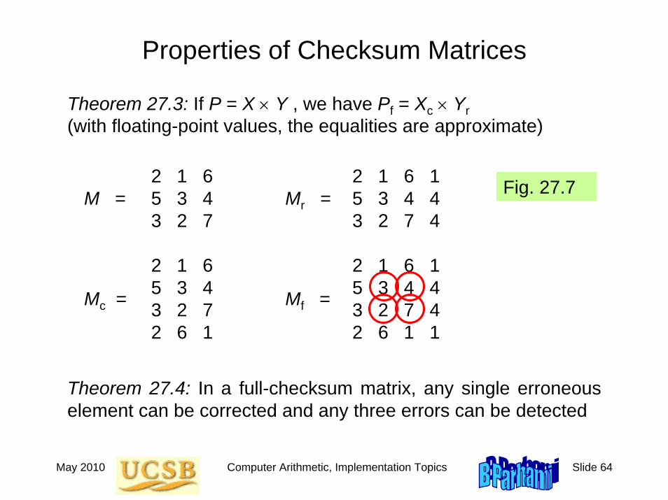
Properties of Checksum Matrices
Theorem 27.3: If P = X × Y , we have Pf = Xc × Yr(with floating-point values, the equalities are approximate)
Theorem 27.4: In a full-checksum matrix, any single erroneous element can be corrected and any three errors can be detected
Fig. 27.72 1 6 2 1 6 1M = 5 3 4 Mr = 5 3 4 4
3 2 7 3 2 7 4
2 1 6 2 1 6 15 3 4 5 3 4 43 2 7 3 2 7 42 6 1 2 6 1 1
Mc = Mf =
May 2010 Computer Arithmetic, Implementation Topics Slide 65
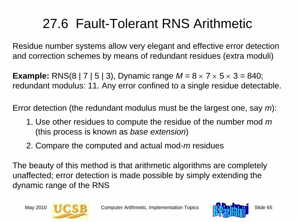
27.6 Fault-Tolerant RNS ArithmeticResidue number systems allow very elegant and effective error detection and correction schemes by means of redundant residues (extra moduli)
Example: RNS(8 | 7 | 5 | 3), Dynamic range M = 8 × 7 × 5 × 3 = 840; redundant modulus: 11. Any error confined to a single residue detectable.
Error detection (the redundant modulus must be the largest one, say m):
1. Use other residues to compute the residue of the number mod m(this process is known as base extension)
2. Compare the computed and actual mod-m residues
The beauty of this method is that arithmetic algorithms are completely unaffected; error detection is made possible by simply extending the dynamic range of the RNS
May 2010 Computer Arithmetic, Implementation Topics Slide 66
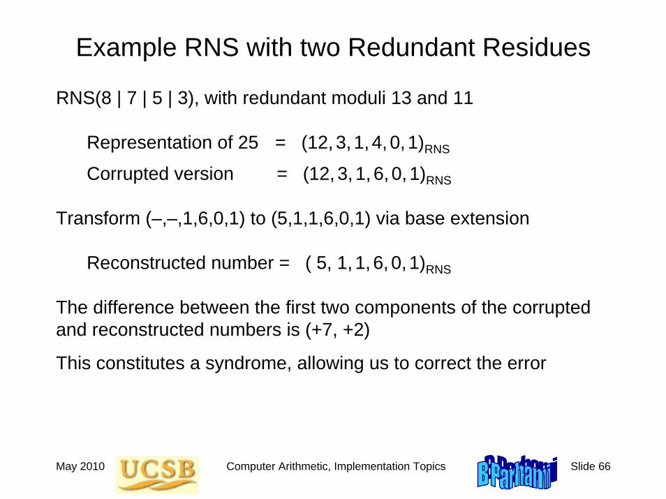
Example RNS with two Redundant Residues
RNS(8 | 7 | 5 | 3), with redundant moduli 13 and 11
Representation of 25 = (12, 3,1,4, 0,1)RNS
Corrupted version = (12, 3, 1, 6,0,1)RNS
Transform (–,–,1,6,0,1) to (5,1,1,6,0,1) via base extension
Reconstructed number = ( 5, 1, 1,6, 0, 1)RNS
The difference between the first two components of the corruptedand reconstructed numbers is (+7, +2)
This constitutes a syndrome, allowing us to correct the error
May 2010 Computer Arithmetic, Implementation Topics Slide 67
28 Reconfigurable Arithmetic
Chapter GoalsExamine arithmetic algorithms and designsappropriate for implementation on FPGAs (one-of-a-kind, low-volume, prototype systems)
Chapter HighlightsSuitable adder designs beyond ripple-carryDesign choices for multipliers and dividersTable-based and “distributed” arithmeticTechniques for function evaluationEnhanced FPGAs and higher-level alternatives
May 2010 Computer Arithmetic, Implementation Topics Slide 68
Reconfigurable Arithmetic: Topics
Topics in This Chapter
28.1 Programmable Logic Devices
28.2 Adder Designs for FPGAs
28.3 Multiplier and Divider Designs
28.4 Tabular and Distributed Arithmetic
28.5 Function Evaluation on FPGAs
28.6 Beyond Fine-Grained Devices
May 2010 Computer Arithmetic, Implementation Topics Slide 69
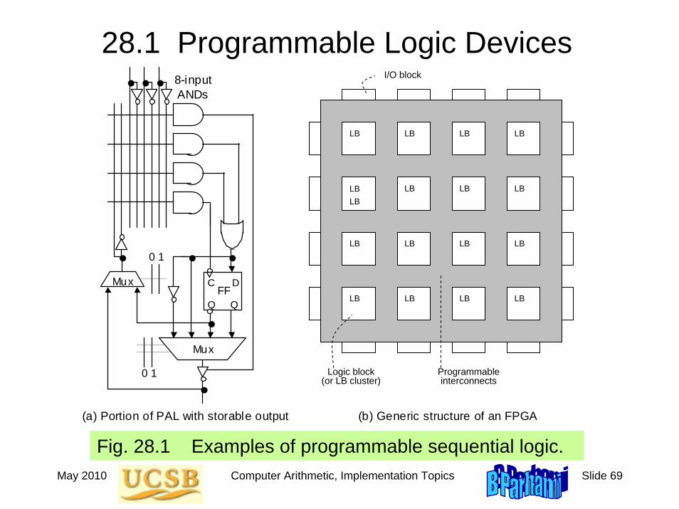
28.1 Programmable Logic Devices
Fig. 28.1 Examples of programmable sequential logic.
(a) Portion of PAL with storable output (b) Generic structure of an FPGA
8-input ANDs
D
C Q
Q
FF
Mux
Mux
0 1
0 1
I/O blocks
Configurable logic block
Programmable connections
CLB
CLB
CLB
CLB
LB LB
LB LB
LB LB LB LB
LB LB LB LB
LBLB
LB LB LB
LB LB LB LB
I/O block
Programmable interconnects
Logic block (or LB cluster)
May 2010 Computer Arithmetic, Implementation Topics Slide 70
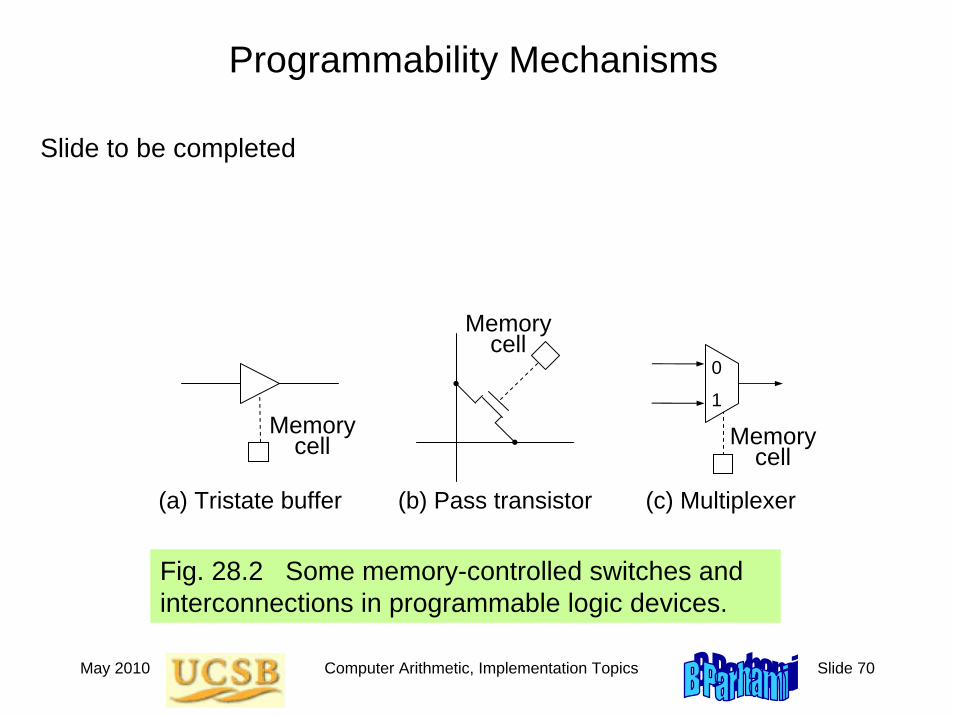
Programmability Mechanisms
Fig. 28.2 Some memory-controlled switches and interconnections in programmable logic devices.
(a) Tristate buffer
0
1
(b) Pass transistor (c) Multiplexer
Memory cell
Memory cell
Memory cell
Slide to be completed
May 2010 Computer Arithmetic, Implementation Topics Slide 71
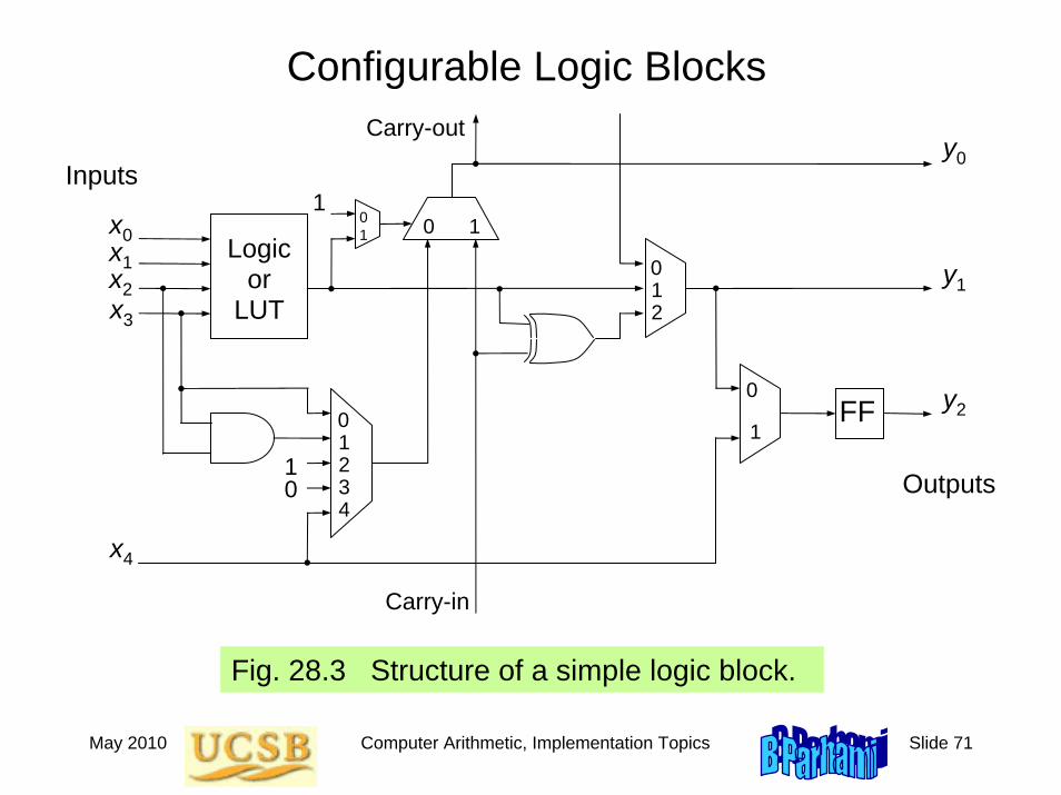
Configurable Logic Blocks
Fig. 28.3 Structure of a simple logic block.
Inputs
FF
Carry-in
Carry-out
Outputs
Logic or
LUT
0
1
0 1
012
10
01234
1
y0
y1
y2
x0x1x2x3
x4
01
May 2010 Computer Arithmetic, Implementation Topics Slide 72
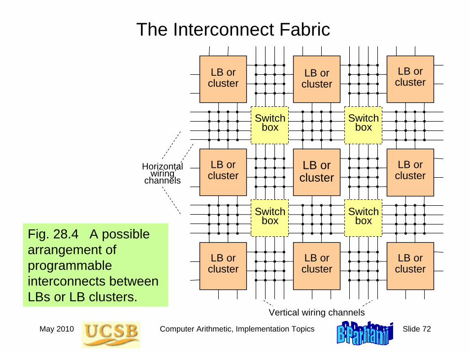
The Interconnect Fabric
Fig. 28.4 A possible arrangement of programmable interconnects between LBs or LB clusters.
LB or cluster
Vertical wiring channels
LB or cluster
LB or cluster
LB or cluster
LB or cluster
LB or cluster
LB or cluster
LB or cluster
LB or cluster
Switch box
Switch box
Switch box
Horizontal wiring
channels
Switch box
May 2010 Computer Arithmetic, Implementation Topics Slide 73
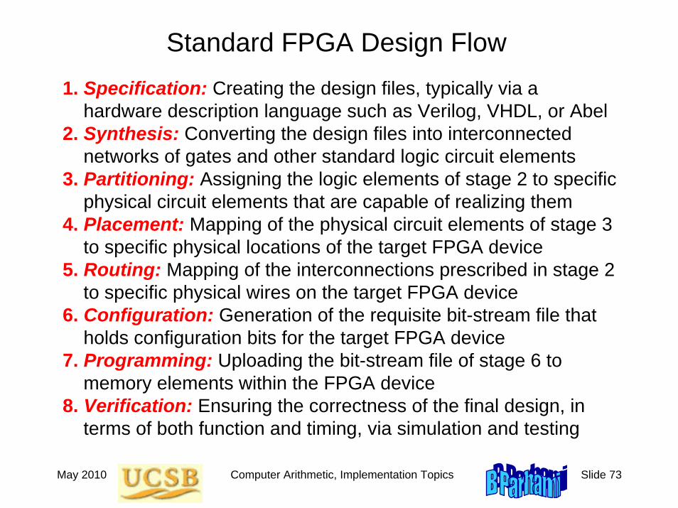
Standard FPGA Design Flow1. Specification: Creating the design files, typically via a
hardware description language such as Verilog, VHDL, or Abel2. Synthesis: Converting the design files into interconnected
networks of gates and other standard logic circuit elements3. Partitioning: Assigning the logic elements of stage 2 to specific
physical circuit elements that are capable of realizing them4. Placement: Mapping of the physical circuit elements of stage 3
to specific physical locations of the target FPGA device5. Routing: Mapping of the interconnections prescribed in stage 2
to specific physical wires on the target FPGA device6. Configuration: Generation of the requisite bit-stream file that
holds configuration bits for the target FPGA device7. Programming: Uploading the bit-stream file of stage 6 to
memory elements within the FPGA device8. Verification: Ensuring the correctness of the final design, in
terms of both function and timing, via simulation and testing
May 2010 Computer Arithmetic, Implementation Topics Slide 74
28.2 Adder Designs for FPGAs
This slide to include a discussion of ripple-carry adders and built-in carry chains in FPGAs
May 2010 Computer Arithmetic, Implementation Topics Slide 75
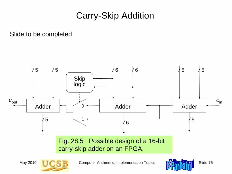
Carry-Skip Addition
Fig. 28.5 Possible design of a 16-bit carry-skip adder on an FPGA.
/ 5 / 5 / 5
0
1
Skiplogic
/ 5/ 6 / 6
/ 5 / 5
cout cinAdder AdderAdder
Slide to be completed
/ 6
May 2010 Computer Arithmetic, Implementation Topics Slide 76
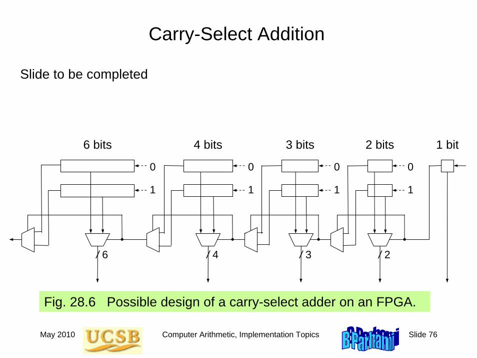
Carry-Select Addition
Fig. 28.6 Possible design of a carry-select adder on an FPGA.
/ 2
2 bits
0
1
0
1
0
1
0
1
3 bits4 bits6 bits 1 bit
/ 3/ 4/ 6
Slide to be completed
May 2010 Computer Arithmetic, Implementation Topics Slide 77
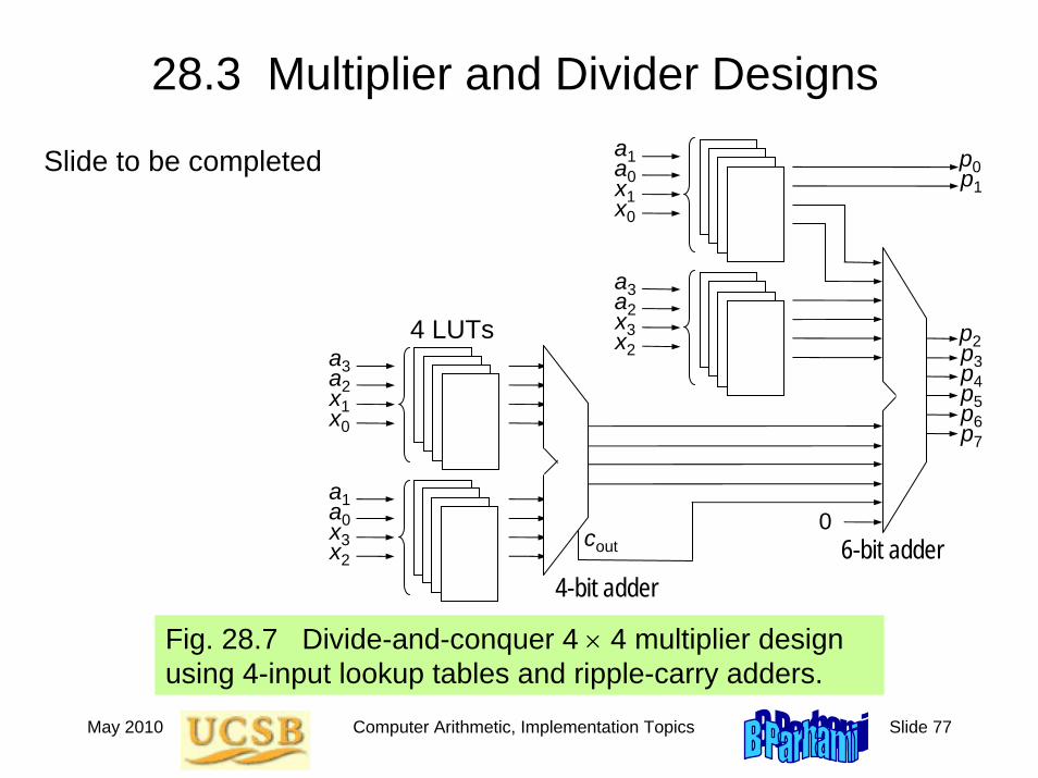
28.3 Multiplier and Divider Designs
Fig. 28.7 Divide-and-conquer 4 × 4 multiplier design using 4-input lookup tables and ripple-carry adders.
a3a2x1x0
4 LUTs
a1a0x3x2
a1a0x1x0
a3a2x3x2
p0p1
0
4-bit adder6-bit adder
p2p3p4p5p6p7
cout
Slide to be completed
May 2010 Computer Arithmetic, Implementation Topics Slide 78
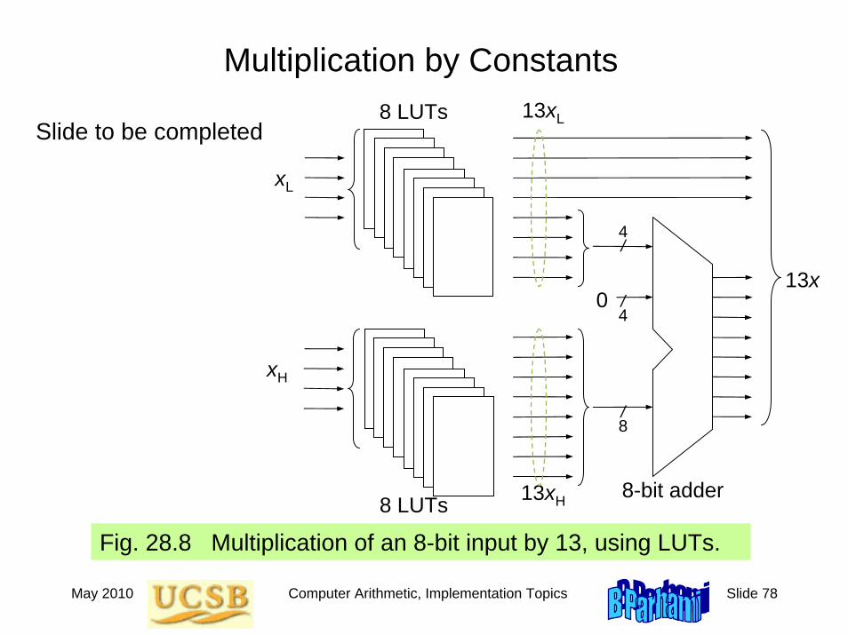
Multiplication by Constants
Fig. 28.8 Multiplication of an 8-bit input by 13, using LUTs.
xL
8 LUTs
0
xH
8 LUTs
4/
/4
/8
13xH
13x
13xL
8-bit adder
Slide to be completed
0
May 2010 Computer Arithmetic, Implementation Topics Slide 79
Division on FPGAs
Slide to be completed
May 2010 Computer Arithmetic, Implementation Topics Slide 80
28.4 Tabular and Distributed Arithmetic
Slide to be completed
May 2010 Computer Arithmetic, Implementation Topics Slide 81
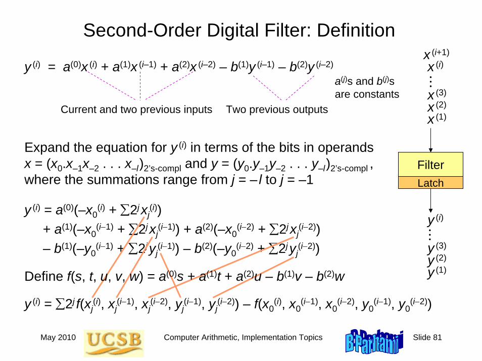
Second-Order Digital Filter: Definition
Current and two previous inputs
y (i) = a(0)x (i) + a(1)x (i–1) + a(2)x (i–2) – b(1)y (i–1) – b(2)y (i–2)
Expand the equation for y (i) in terms of the bits in operands x = (x0.x–1x–2 . . . x–l)2’s-compl and y = (y0.y–1y–2 . . . y–l)2’s-compl , where the summations range from j = – l to j = –1
y (i) = a(0)(–x0(i) + ∑2j xj
(i)) + a(1)(–x0
(i−1) + ∑2j xj(i−1)) + a(2)(–x0
(i−2) + ∑2j xj(i−2))
– b(1)(–y0(i−1) + ∑2j yj
(i−1)) – b(2)(–y0(i−2) + ∑2j yj
(i−2))
FilterLatch
x (1)x (2)x (3)
x (i)...
y (1)y (2)y (3)
y (i)...
x (i+1)
Two previous outputs
a(j)s and b(j)s are constants
Define f(s, t, u, v, w) = a(0)s + a(1)t + a(2)u – b(1)v – b(2)w
y (i) = ∑2j f(xj(i), xj
(i−1), xj(i−2), yj
(i−1), yj(i−2)) – f(x0
(i), x0(i−1), x0
(i−2), y0(i−1), y0
(i−2))
May 2010 Computer Arithmetic, Implementation Topics Slide 82
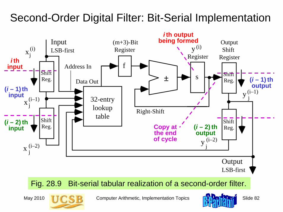
Second-Order Digital Filter: Bit-Serial Implementation
Fig. 28.9 Bit-serial tabular realization of a second-order filter.
f
x
x
x
(i)
(i–1)
(i–2)
j
j
j
y (i–1)j
y (i–2)j
LSB-first y (i)
±
Input
32-Entry Table (ROM)
Output Shift Register
(m+3)-Bit Register
Data Out
Address In
s
Right-Shift
LSB-firstOutput
ShiftReg.
ShiftReg.
ShiftReg.
ShiftReg.
Registeri th input
(i – 1) th input
(i – 2) th input
(i – 1) th output
i th output being formed
(i – 2) th output
Copy at the end of cycle
32-entry lookuptable
May 2010 Computer Arithmetic, Implementation Topics Slide 83
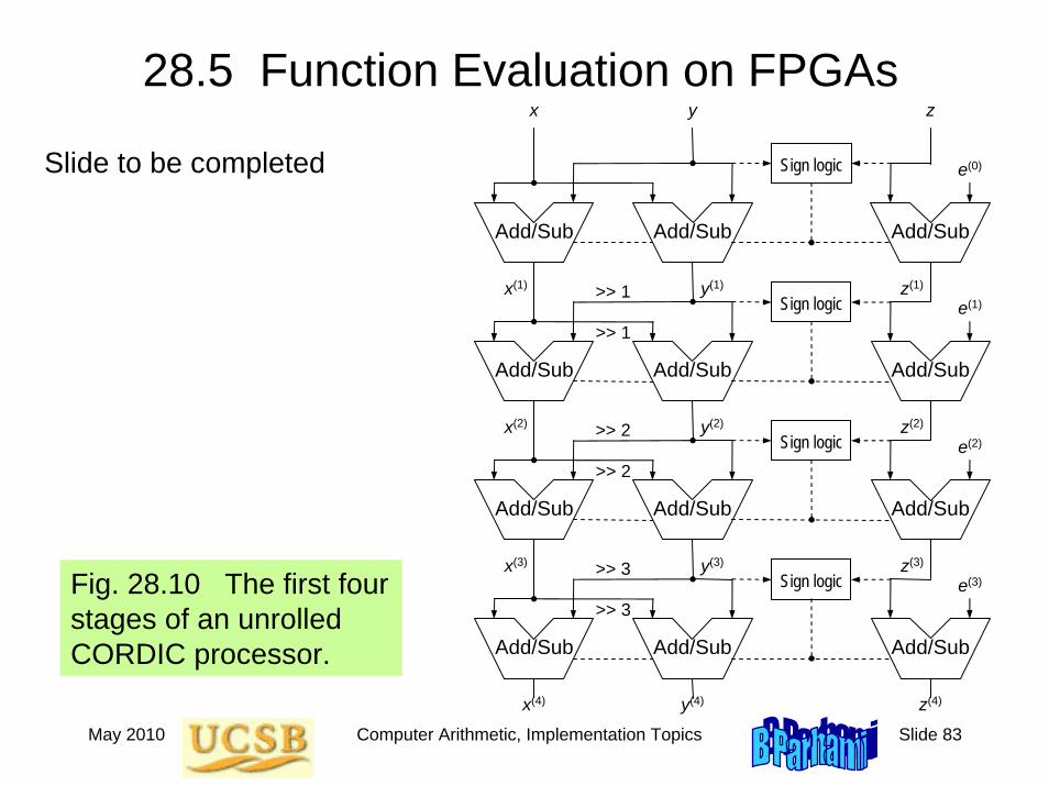
28.5 Function Evaluation on FPGAs
Fig. 28.10 The first four stages of an unrolled CORDIC processor.
Add/Sub Add/Sub
Add/Sub Add/Sub
>> 1
>> 1
Add/Sub Add/Sub
>> 2
>> 2
Add/Sub Add/Sub
>> 3
>> 3
Add/Sub
Add/Sub
Add/Sub
Add/Sub
Sign logic
Sign logic
Sign logic
Sign logic
e(0)
e(1)
e(2)
e(3)
x y z
z(4)x(4) y(4)
z(3)x(3) y(3)
x(2) y(2)
x(1) y(1)
z(2)
z(1)
Slide to be completed
May 2010 Computer Arithmetic, Implementation Topics Slide 84
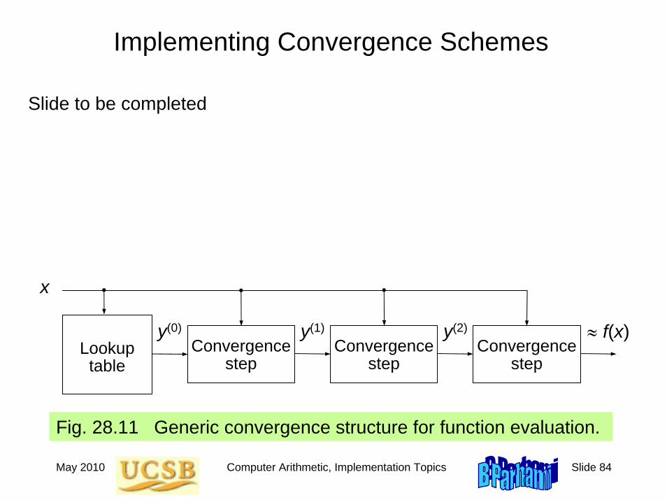
Implementing Convergence Schemes
Fig. 28.11 Generic convergence structure for function evaluation.
Lookup table
x
Convergence step
y(0) ≈ f(x)Convergence
step Convergence
step
y(1) y(2)
Slide to be completed
May 2010 Computer Arithmetic, Implementation Topics Slide 85
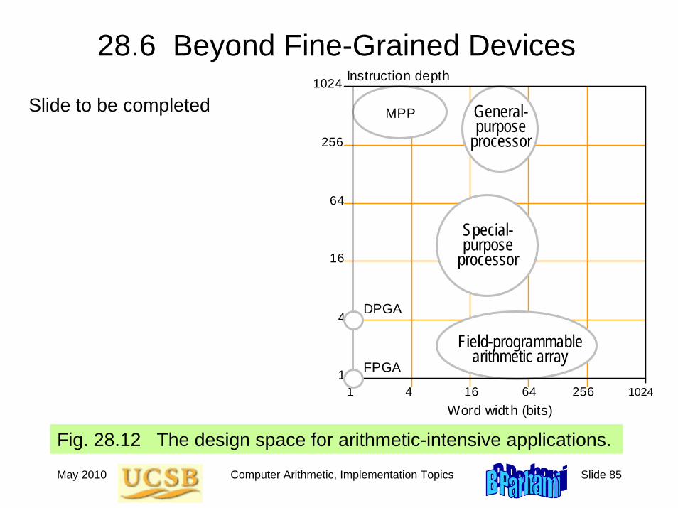
28.6 Beyond Fine-Grained Devices
Fig. 28.12 The design space for arithmetic-intensive applications.Word width (bits)
1 4 64 16 256 10241
4
64
16
256
1024 Instruction depth
FPGA
DPGA
GP micro
Our approach
MPP
SP processor
General-purpose
processor
Special-purpose
processor
Field-programmable arithmetic array
1024
Slide to be completed
May 2010 Computer Arithmetic, Implementation Topics Slide 86
A Past, Present, and Future
Appendix GoalsWrap things up, provide perspective, andexamine arithmetic in a few key systems
Appendix HighlightsOne must look at arithmetic in context of
• Computational requirements• Technological constraints• Overall system design goals• Past and future developments
Current trends and research directions?
May 2010 Computer Arithmetic, Implementation Topics Slide 87
Past, Present, and Future: Topics
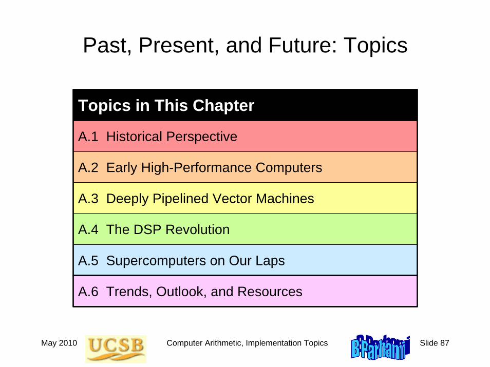
Topics in This Chapter
A.1 Historical Perspective
A.2 Early High-Performance Computers
A.3 Deeply Pipelined Vector Machines
A.4 The DSP Revolution
A.5 Supercomputers on Our Laps
A.6 Trends, Outlook, and Resources
May 2010 Computer Arithmetic, Implementation Topics Slide 88
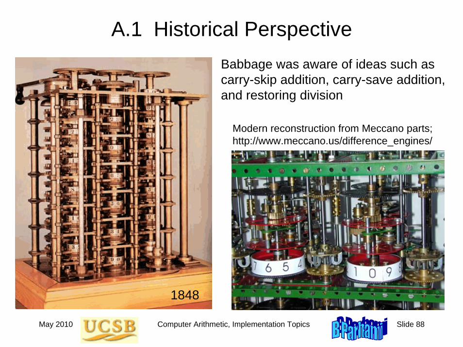
A.1 Historical PerspectiveBabbage was aware of ideas such as carry-skip addition, carry-save addition, and restoring division
1848
Modern reconstruction from Meccano parts;http://www.meccano.us/difference_engines/
May 2010 Computer Arithmetic, Implementation Topics Slide 89
Computer Arithmetic in the 1940s
Machine arithmetic was crucial in proving the feasibility of computing with stored-program electronic devices
Hardware for addition/subtraction, use of complement representation, and shift-add multiplication and division algorithms were developed and fine-tuned
A seminal report by A.W. Burkes, H.H. Goldstein, and J. von Neumann contained ideas on choice of number radix, carry propagation chains, fast multiplication via carry-save addition, and restoring division
State of computer arithmetic circa 1950: Overview paper by R.F. Shaw [Shaw50]
May 2010 Computer Arithmetic, Implementation Topics Slide 90
Computer Arithmetic in the 1950s
The focus shifted from feasibility to algorithmic speedup methods and cost-effective hardware realizations
By the end of the decade, virtually all important fast-adder designs had already been published or were in the final phases of development
Residue arithmetic, SRT division, CORDIC algorithms were proposed and implemented
Snapshot of the field circa 1960: Overview paper by O.L. MacSorley [MacS61]
May 2010 Computer Arithmetic, Implementation Topics Slide 91
Computer Arithmetic in the 1960s
Tree multipliers, array multipliers, high-radix dividers, convergence division, redundant signed-digit arithmetic were introduced
Implementation of floating-point arithmetic operations in hardware or firmware (in microprogram) became prevalent
Many innovative ideas originated from the design of early supercomputers, when the demand for high performance, along with the still high cost of hardware, led designers to novel and cost-effective solutions
Examples reflecting the sate of the art near the end of this decade:IBM’s System/360 Model 91 [Ande67] Control Data Corporation’s CDC 6600 [Thor70]
May 2010 Computer Arithmetic, Implementation Topics Slide 92
Computer Arithmetic in the 1970s
Advent of microprocessors and vector supercomputers
Early LSI chips were quite limited in the number of transistors or logic gates that they could accommodate
Microprogrammed control (with just a hardware adder) was a natural choice for single-chip processors which were not yet expected to offer high performance
For high end machines, pipelining methods were perfected to allow the throughput of arithmetic units to keep up with computationaldemand in vector supercomputers
Examples reflecting the state of the art near the end of this decade:Cray 1 supercomputer and its successors
May 2010 Computer Arithmetic, Implementation Topics Slide 93
Computer Arithmetic in the 1980s
Spread of VLSI triggered a reconsideration of all arithmetic designs in light of interconnection cost and pin limitations
For example, carry-lookahead adders, thought to be ill-suited to VLSI, were shown to be efficiently realizable after suitable modifications. Similar ideas were applied to more efficient VLSI tree and arraymultipliers
Bit-serial and on-line arithmetic were advanced to deal with severe pin limitations in VLSI packages
Arithmetic-intensive signal processing functions became driving forces for low-cost and/or high-performance embedded hardware: DSP chips
May 2010 Computer Arithmetic, Implementation Topics Slide 94
Computer Arithmetic in the 1990s
No breakthrough design concept
Demand for performance led to fine-tuning of arithmetic algorithms and implementations (many hybrid designs)
Increasing use of table lookup and tight integration of arithmetic unit and other parts of the processor for maximum performance
Clock speeds reached and surpassed 100, 200, 300, 400, and 500 MHz in rapid succession; pipelining used to ensure smooth flow of data through the system
Examples reflecting the state of the art near the end of this decade:Intel’s Pentium Pro (P6) → Pentium IISeveral high-end DSP chips
May 2010 Computer Arithmetic, Implementation Topics Slide 95
Computer Arithmetic in the 2000s
Continued refinement of many existing methods, particularly those based on table lookup
New challenges posed by multi-GHz clock rates
Increased emphasis on low-power design
Work on, and approval of, the IEEE 754-2008 floating-point standard
Three parallel and interacting trends:Availability of many millions of transistors on a single microchipEnergy requirements and heat dissipation of the said transistorsShift of focus from scientific computations to media processing
May 2010 Computer Arithmetic, Implementation Topics Slide 96
A.2 Early High-Performance Computers
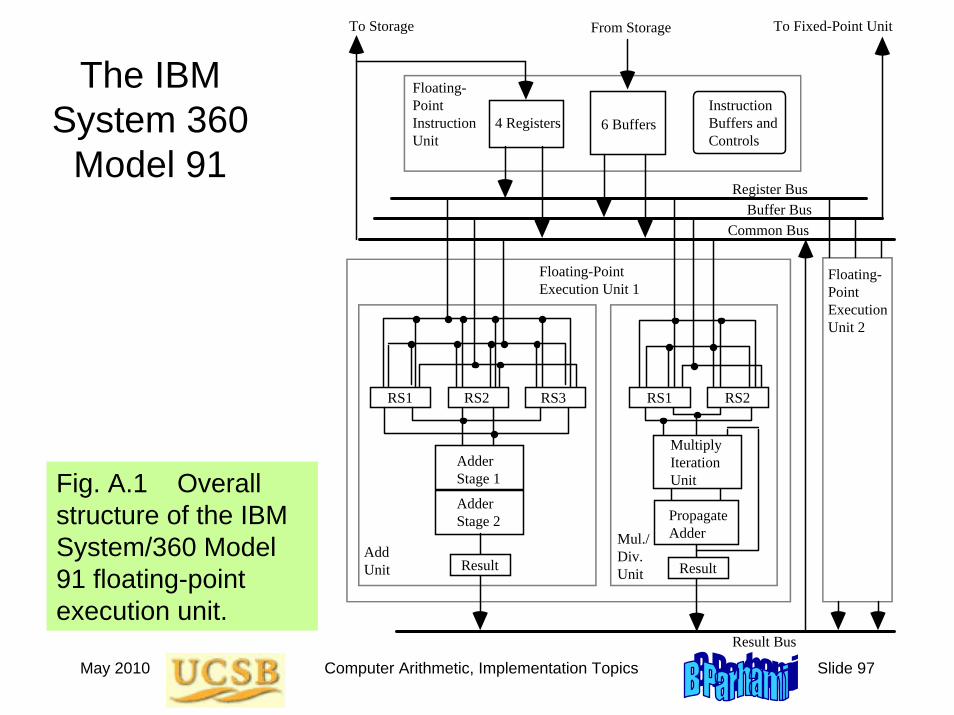
IBM System 360 Model 91 (360/91, for short; mid 1960s)
Part of a family of machines with the same instruction-set architecture
Had multiple function units and an elaborate scheduling and interlocking hardware algorithm to take advantage of them for high performance
Clock cycle = 20 ns (quite aggressive for its day)
Used 2 concurrently operating floating-point execution units performing:
Two-stage pipelined addition
12 × 56 pipelined partial-tree multiplication
Division by repeated multiplications (initial versions of the machine sometimes yielded an incorrect LSB for the quotient)
May 2010 Computer Arithmetic, Implementation Topics Slide 97
The IBM System 360
Model 91
Fig. A.1 Overall structure of the IBM System/360 Model 91 floating-point execution unit.
Floating- Point Instruction Unit
RS1 RS2 RS3 RS1 RS2
Register BusBuffer Bus
Common Bus
Instruction Buffers and Controls
4 Registers 6 Buffers
To Storage
Adder Stage 1
Adder Stage 2
Result Bus
Result Result
Multiply Iteration Unit
Propagate Adder
From Storage To Fixed-Point Unit
Add Unit
Mul./ Div. Unit
Floating-Point Execution Unit 1
Floating- Point Execution Unit 2
May 2010 Computer Arithmetic, Implementation Topics Slide 98
A.3 Deeply Pipelined Vector Machines
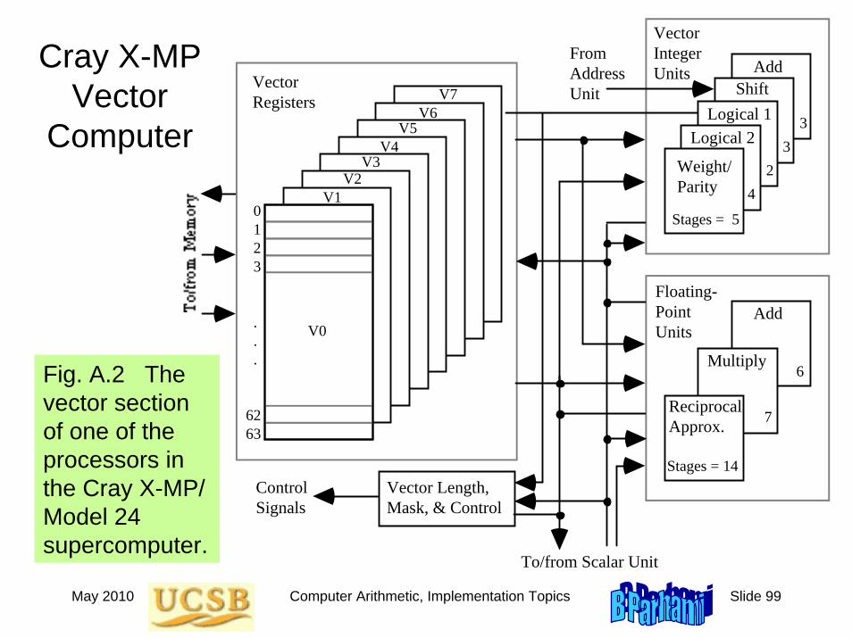
Cray X-MP/Model 24 (multiple-processor vector machine)
Had multiple function units, each of which could produce a new result on every clock tick, given suitably long vectors to process
Clock cycle = 9.5 ns
Used 5 integer/logic function units and 3 floating-point function units
Integer/Logic units: add, shift, logical 1, logical 2, weight/parity
Floating-point units: add (6 stages), multiply (7 stages), reciprocal approximation (14 stages)
Pipeline setup and shutdown overheads
Vector unit not efficient for short vectors (break-even point)
Pipeline chaining
May 2010 Computer Arithmetic, Implementation Topics Slide 99
Cray X-MP Vector
Computer
Fig. A.2 The vector section of one of the processors in the Cray X-MP/ Model 24 supercomputer.
V0
V7V6
V5V4
V3V2
V1 0 1 2 3 . . . 62 63
Vector Registers
Vector Integer Units
Logical 1Shift
Add
Logical 2
Weight/ Parity
Stages = 5
42
33
Floating- Point Units
Multiply
Add
Reciprocal Approx.
Stages = 14
7
6
To/from Scalar Unit
Vector Length, Mask, & Control
From Address Unit
Control Signals
May 2010 Computer Arithmetic, Implementation Topics Slide 100
A.4 The DSP Revolution
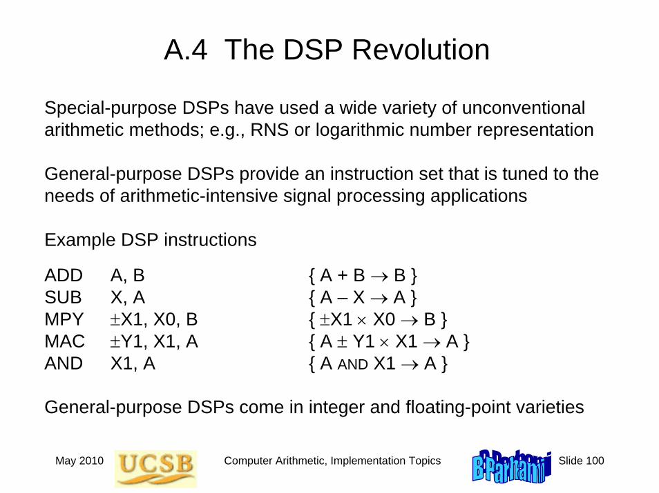
Special-purpose DSPs have used a wide variety of unconventional arithmetic methods; e.g., RNS or logarithmic number representation
General-purpose DSPs provide an instruction set that is tuned to the needs of arithmetic-intensive signal processing applications
Example DSP instructions
ADD A, B { A + B → B }SUB X, A { A – X → A }MPY ±X1, X0, B { ±X1 × X0 → B }MAC ±Y1, X1, A { A ± Y1 × X1 → A }AND X1, A { A AND X1 → A }
General-purpose DSPs come in integer and floating-point varieties
May 2010 Computer Arithmetic, Implementation Topics Slide 101
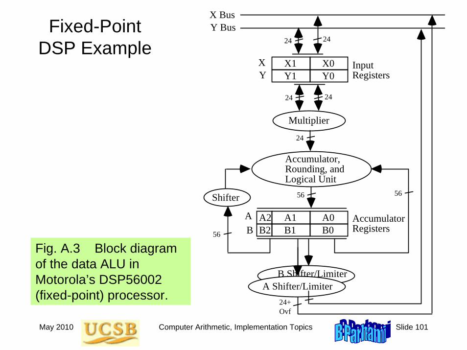
Fixed-Point DSP Example
Fig. A.3 Block diagram of the data ALU in Motorola’s DSP56002 (fixed-point) processor.
B Shifter/Limiter
X BusY Bus
X1 X0Y1 Y0
XY
24 24
24 24
24
A1 A0B1 B0
AB
A2B2
56 56Shifter
56
A Shifter/Limiter
Accumulator, Rounding, and Logical Unit
Multiplier
Input Registers
Accumulator Registers
24+ Ovf
May 2010 Computer Arithmetic, Implementation Topics Slide 102
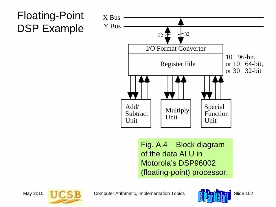
Floating-Point DSP Example
Fig. A.4 Block diagram of the data ALU in Motorola’s DSP96002 (floating-point) processor.
I/O Format Converter
X BusY Bus
32 32
Register File10 96-bit, or 10 64-bit, or 30 32-bit
Add/ Subtract Unit
Multiply Unit
Special Function Unit
May 2010 Computer Arithmetic, Implementation Topics Slide 103
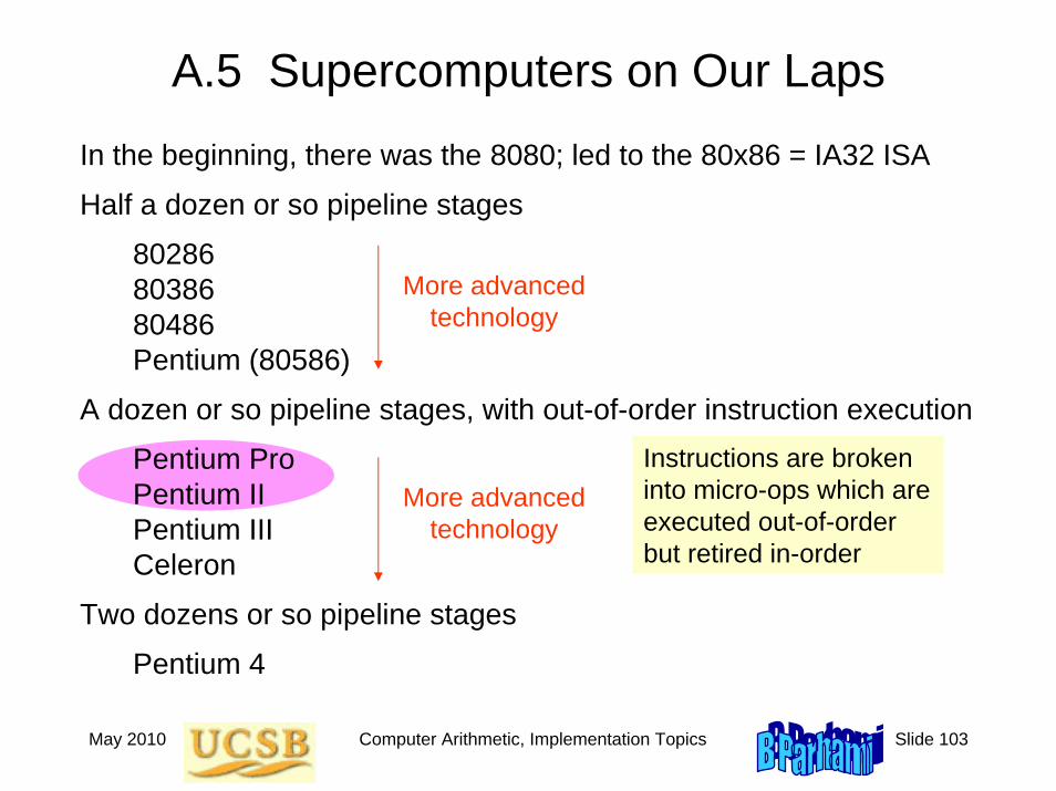
A.5 Supercomputers on Our Laps
In the beginning, there was the 8080; led to the 80x86 = IA32 ISA
Half a dozen or so pipeline stages
802868038680486Pentium (80586)
A dozen or so pipeline stages, with out-of-order instruction execution
Pentium ProPentium IIPentium IIICeleron
Two dozens or so pipeline stages
Pentium 4
More advanced technology
More advanced technology
Instructions are broken into micro-ops which are executed out-of-order but retired in-order
May 2010 Computer Arithmetic, Implementation Topics Slide 104
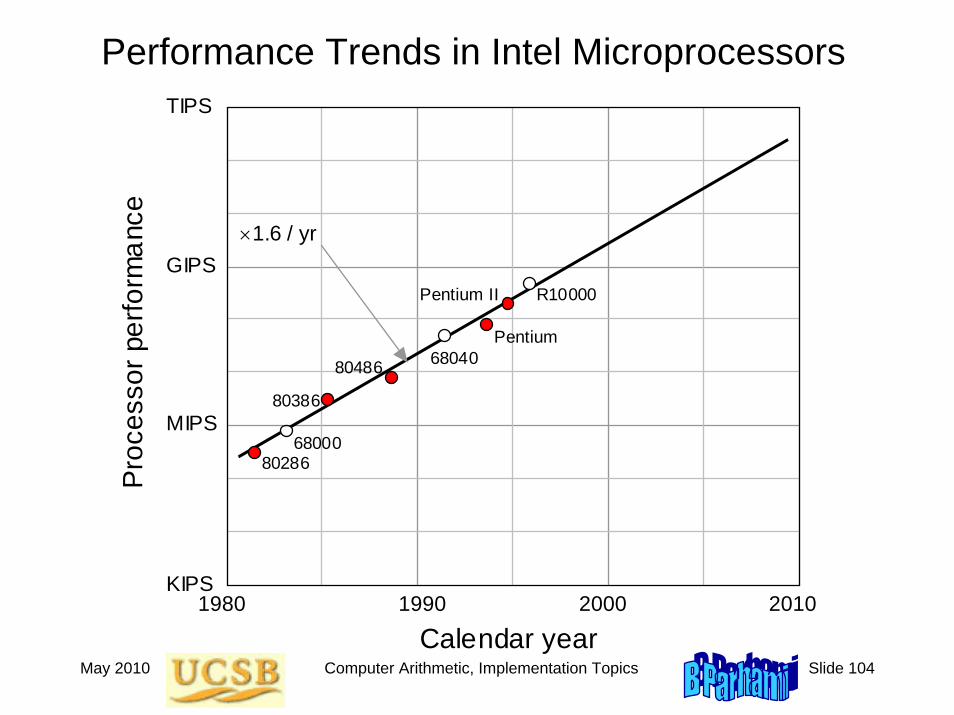
Performance Trends in Intel Microprocessors
1990 1980 2000 2010 KIPS
MIPS
GIPS
TIPS P
roce
ssor
per
form
ance
Calendar year
80286 68000
80386
80486 68040 Pentium
Pentium II R10000
×1.6 / yr
May 2010 Computer Arithmetic, Implementation Topics Slide 105
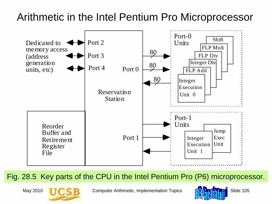
Arithmetic in the Intel Pentium Pro Microprocessor
Integer Execution Unit 0
80 80
80
Port-0 Units
Port-1 Units
Port 0
Port 1
Port 2
Dedicated to memory access (address generation units, etc)
Port 3 Port 4
Reservation Station
Reorder Buffer and Retirement Register File
FLP Add
Integer Div
FLP Div
FLP Mult
Shift
Integer Execution Unit 1
Jump Exec Unit
Fig. 28.5 Key parts of the CPU in the Intel Pentium Pro (P6) microprocessor.
May 2010 Computer Arithmetic, Implementation Topics Slide 106
A.6 Trends, Outlook, and Resources
Current focus areas in computer arithmetic
Design: Shift of attention from algorithms to optimizations at the level of transistors and wires
This explains the proliferation of hybrid designs
Technology: Predominantly CMOS, with a phenomenal rate of improvement in size/speed
New technologies cannot compete
Applications: Shift from high-speed or high-throughput designs in mainframes to embedded systems requiring
Low costLow power
May 2010 Computer Arithmetic, Implementation Topics Slide 107
Ongoing Debates and New Paradigms
Renewed interest in bit- and digit-serial arithmetic as mechanisms to reduce the VLSI area and to improve packageability and testability
Synchronous vs asynchronous design (asynchrony has some overhead, but an equivalent overhead is being paid for clock distribution and/or systolization)
New design paradigms may alter the way in which we view or design arithmetic circuits
Neuronlike computational elementsOptical computing (redundant representations) Multivalued logic (match to high-radix arithmetic)Configurable logic
Arithmetic complexity theory
May 2010 Computer Arithmetic, Implementation Topics Slide 108
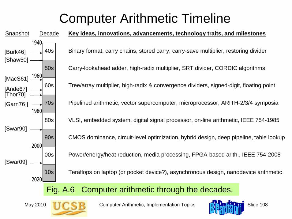
Computer Arithmetic Timeline
Fig. A.6 Computer arithmetic through the decades.
Decade
40s
50s
60s
70s
80s
90s
00s
10s
1940
2020
1960
1980
2000
Snapshot
[Burk46]
Key ideas, innovations, advancements, technology traits, and milestones
Binary format, carry chains, stored carry, carry-save multiplier, restoring divider[Shaw50]
Carry-lookahead adder, high-radix multiplier, SRT divider, CORDIC algorithms
Tree/array multiplier, high-radix & convergence dividers, signed-digit, floating point
Pipelined arithmetic, vector supercomputer, microprocessor, ARITH-2/3/4 symposia
VLSI, embedded system, digital signal processor, on-line arithmetic, IEEE 754-1985
CMOS dominance, circuit-level optimization, hybrid design, deep pipeline, table lookup
Power/energy/heat reduction, media processing, FPGA-based arith., IEEE 754-2008
Teraflops on laptop (or pocket device?), asynchronous design, nanodevice arithmetic
[MacS61]
[Thor70][Ande67]
[Swar90]
[Swar09]
[Garn76]]

May 2010 Computer Arithmetic, Implementation Topics Slide 109
The End!
You’re up to date. Take my advice and try to keep it that way. It’ll be tough to do; make no mistake about it. The phone will ring and it’ll be the administrator –– talking about budgets. The doctors will come in, and they’ll want this bit of information and that. Then you’ll get the salesman. Until at the end of the day you’ll wonder what happened to it and what you’ve accomplished; what you’ve achieved.That’s the way the next day can go, and the next, and the one after that. Until you find a year has slipped by, and another, and another. And then suddenly, one day, you’ll find everything you knew is out of date. That’s when it’s too late to change.Listen to an old man who’s been through it all, who made the mistake of falling behind. Don’t let it happen to you! Lock yourself in a closet if you have to! Get away from the phone and the files and paper, and read and learn and listen and keep up to date. Then they can never touch you, never say, “He’s finished, all washed up; he belongs to yesterday.”
Arthur Hailey, The Final Diagnosis