Embed Size (px)
Citation preview
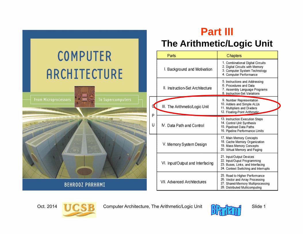
Oct. 2014 Computer Architecture, The Arithmetic/Logic Unit Slide 1
Part IIIThe Arithmetic/Logic Unit
Oct. 2014 Computer Architecture, The Arithmetic/Logic Unit Slide 2
About This PresentationThis presentation is intended to support the use of the textbook Computer Architecture: From Microprocessors to Supercomputers, Oxford University Press, 2005, ISBN 0-19-515455-X. It is updated regularly by the author as part of his teaching of the upper-division course ECE 154, Introduction to Computer Architecture, at the University of California, Santa Barbara. Instructors can use these slides freely in classroom teaching and for other educational purposes. Any other use is strictly prohibited. © Behrooz Parhami
Edition Released Revised Revised Revised RevisedFirst July 2003 July 2004 July 2005 Mar. 2006 Jan. 2007
Jan. 2008 Jan. 2009 Jan. 2011 Oct. 2014

Oct. 2014 Computer Architecture, The Arithmetic/Logic Unit Slide 3
III The Arithmetic/Logic Unit
Topics in This PartChapter 9 Number RepresentationChapter 10 Adders and Simple ALUsChapter 11 Multipliers and DividersChapter 12 Floating-Point Arithmetic
Overview of computer arithmetic and ALU design:• Review representation methods for signed integers• Discuss algorithms & hardware for arithmetic ops• Consider floating-point representation & arithmetic
Oct. 2014 Computer Architecture, The Arithmetic/Logic Unit Slide 4
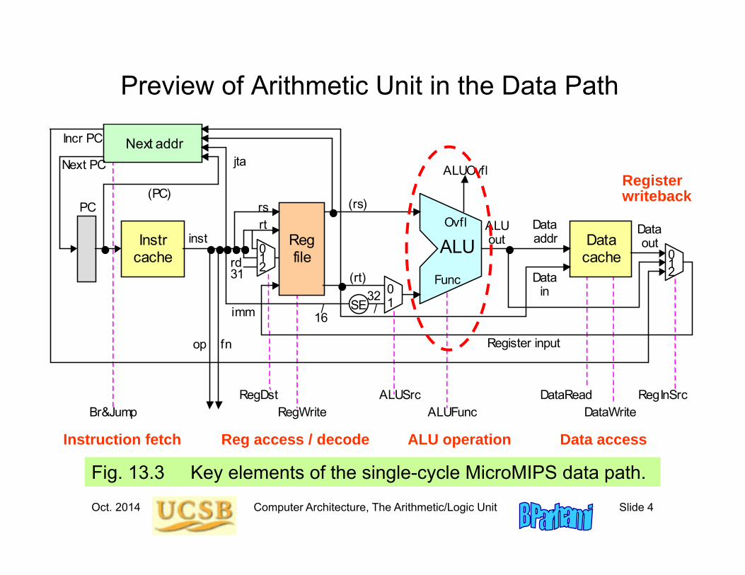
Preview of Arithmetic Unit in the Data Path
Fig. 13.3 Key elements of the single-cycle MicroMIPS data path.
/
ALU
Data cache
Instr cache
Next addr
Reg file
op
jta
fn
inst
imm
rs (rs)
(rt)
Data addr
Data in 0
1
ALUSrc ALUFunc DataWrite
DataRead
SE
RegInSrc
rt
rd
RegDst RegWrite
32 / 16
Register input
Data out
Func
ALUOvfl
Ovfl
31
0 1 2
Next PC
Incr PC
(PC)
Br&Jump
ALU out
PC
0 1 2
Instruction fetch Reg access / decode ALU operation Data access
Register writeback
Oct. 2014 Computer Architecture, The Arithmetic/Logic Unit Slide 5
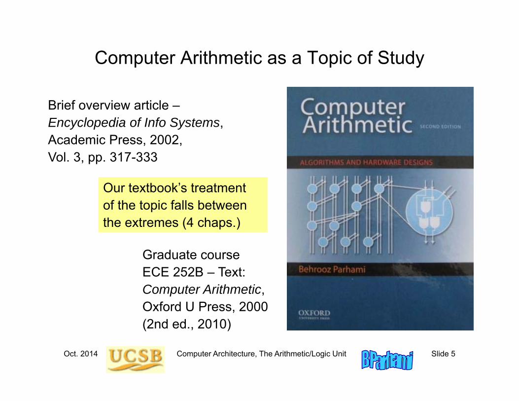
Computer Arithmetic as a Topic of Study
Brief overview article –Encyclopedia of Info Systems,Academic Press, 2002, Vol. 3, pp. 317-333
Our textbook’s treatment of the topic falls between the extremes (4 chaps.)
Graduate courseECE 252B – Text:Computer Arithmetic,Oxford U Press, 2000(2nd ed., 2010)

Oct. 2014 Computer Architecture, The Arithmetic/Logic Unit Slide 6
9 Number RepresentationArguably the most important topic in computer arithmetic:
• Affects system compatibility and ease of arithmetic• Two’s complement, flp, and unconventional methods
Topics in This Chapter9.1 Positional Number Systems9.2 Digit Sets and Encodings9.3 Number-Radix Conversion9.4 Signed Integers9.5 Fixed-Point Numbers9.6 Floating-Point Numbers
Oct. 2014 Computer Architecture, The Arithmetic/Logic Unit Slide 7
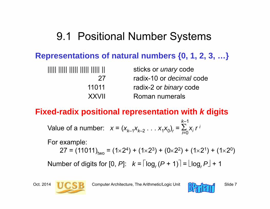
9.1 Positional Number Systems
Representations of natural numbers {0, 1, 2, 3, …}||||| ||||| ||||| ||||| ||||| || sticks or unary code
27 radix-10 or decimal code11011 radix-2 or binary codeXXVII Roman numerals
Fixed-radix positional representation with k digits
Value of a number: x = (xk–1xk–2 . . . x1x0)r = xi r i
For example:27 = (11011)two = (124) + (123) + (022) + (121) + (120)
Number of digits for [0, P]: k = logr (P + 1) = logr P + 1
k–1
i=0
Oct. 2014 Computer Architecture, The Arithmetic/Logic Unit Slide 8
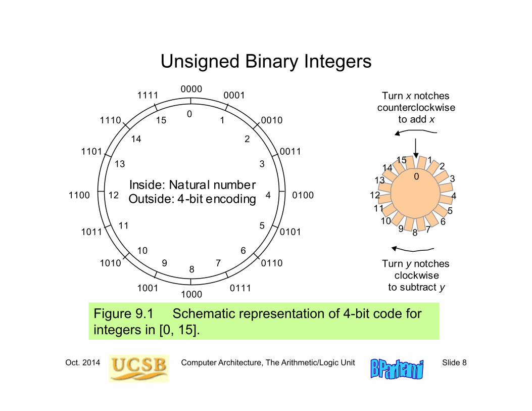
Unsigned Binary Integers
Figure 9.1 Schematic representation of 4-bit code for integers in [0, 15].
0000 0001 1111
0010 1110
0011 1101
0100 1100
1000
0101 1011
0110 1010
0111 1001
0 1
2
3
4
5
6 7
15
11
14
13
12
8 9
10
Inside: Natural number Outside: 4-bit encoding
0
1 2
3
15
4 5
6 7 8 9
Turn x notches counterclockwise
to add x
Turn y notches clockwise
to subtract y
11
14 13
12
10

Oct. 2014 Computer Architecture, The Arithmetic/Logic Unit Slide 9
Representation Range and Overflow
Figure 9.2 Overflow regions in finite number representation systems. For unsigned representations covered in this section, max – = 0.
max
Finite set of representable numbers
Overflow region max Overflow region
Numbers larger than max
Numbers smaller than max
Example 9.2, Part d
Discuss if overflow will occur when computing 317 – 316 in a number system with k = 8 digits in radix r = 10.SolutionThe result 86 093 442 is representable in the number system whichhas a range [0, 99 999 999]; however, if 317 is computed en route to the final result, overflow will occur.
Oct. 2014 Computer Architecture, The Arithmetic/Logic Unit Slide 10
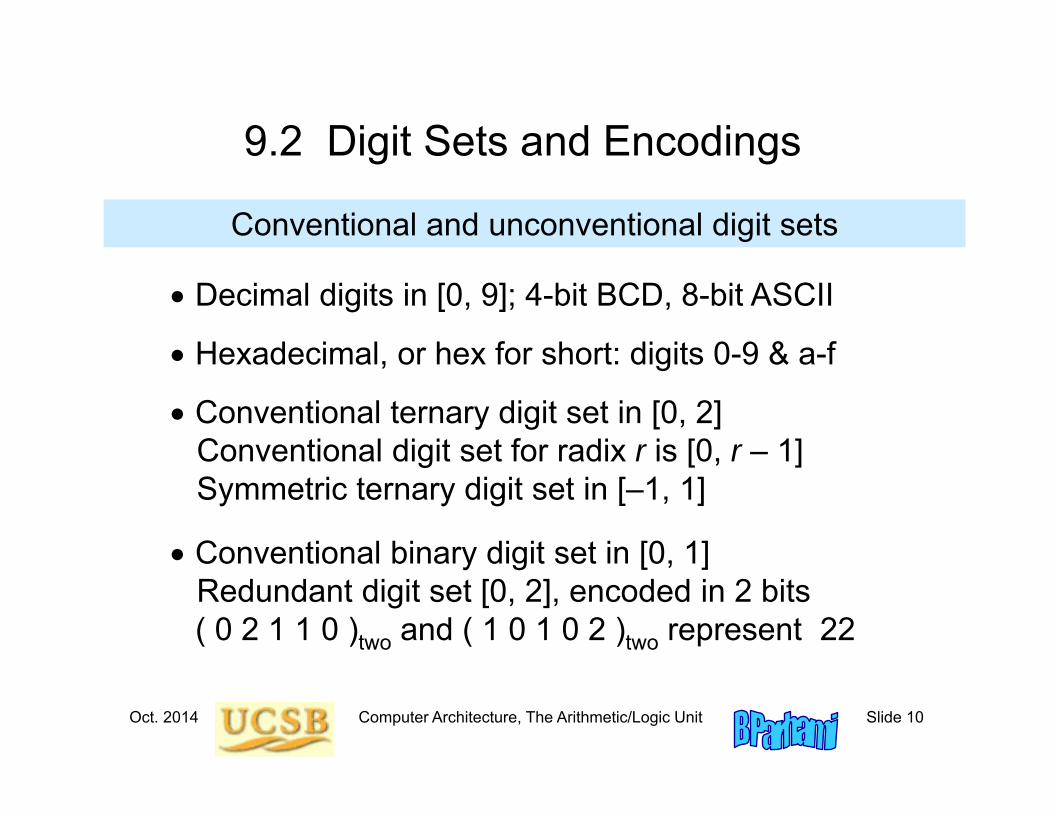
9.2 Digit Sets and Encodings
Conventional and unconventional digit sets
Decimal digits in [0, 9]; 4-bit BCD, 8-bit ASCII
Hexadecimal, or hex for short: digits 0-9 & a-f
Conventional ternary digit set in [0, 2]Conventional digit set for radix r is [0, r – 1]Symmetric ternary digit set in [–1, 1]
Conventional binary digit set in [0, 1]Redundant digit set [0, 2], encoded in 2 bits( 0 2 1 1 0 )two and ( 1 0 1 0 2 )two represent 22
Oct. 2014 Computer Architecture, The Arithmetic/Logic Unit Slide 11
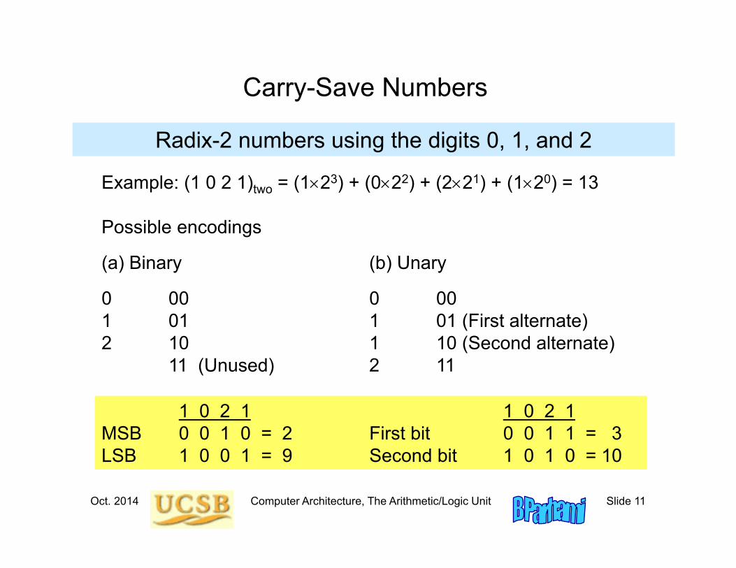
Carry-Save Numbers
Radix-2 numbers using the digits 0, 1, and 2
Example: (1 0 2 1)two = (123) + (022) + (221) + (120) = 13
Possible encodings
(a) Binary (b) Unary
0 00 0 001 01 1 01 (First alternate)2 10 1 10 (Second alternate)
11 (Unused) 2 11
1 0 2 1 1 0 2 1MSB 0 0 1 0 = 2 First bit 0 0 1 1 = 3LSB 1 0 0 1 = 9 Second bit 1 0 1 0 = 10
Oct. 2014 Computer Architecture, The Arithmetic/Logic Unit Slide 12
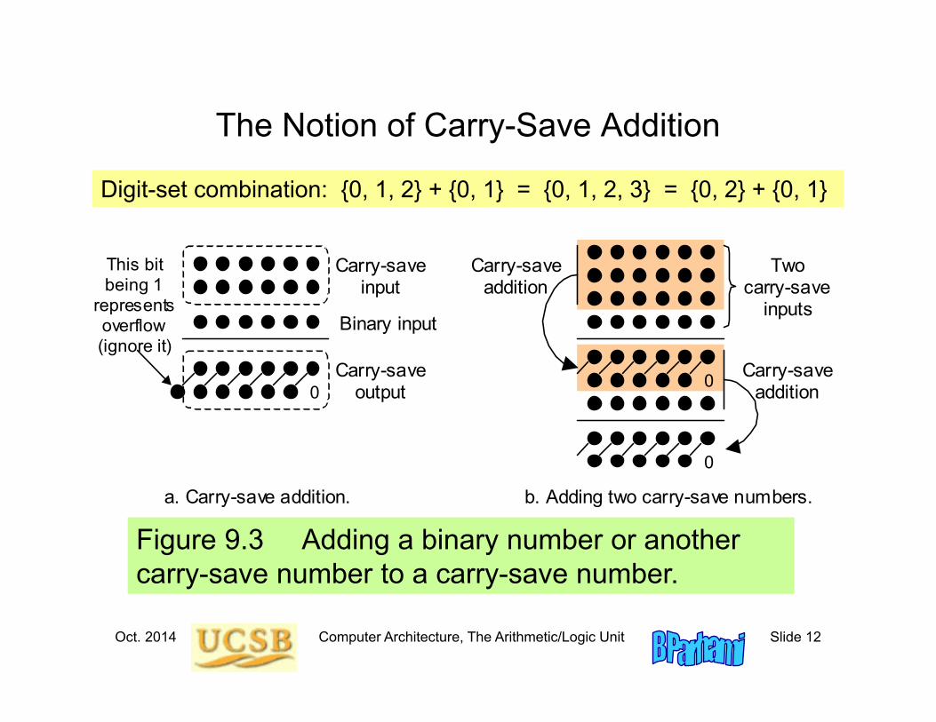
Figure 9.3 Adding a binary number or another carry-save number to a carry-save number.
The Notion of Carry-Save Addition
Two carry-save
inputs
Carry-save input
Binary input
Carry-save output
This bit being 1
represents overflow (ignore it)
0 0
0
a. Carry-save addition. b. Adding two carry-save numbers.
Carry-save addition
Carry-saveaddition
Digit-set combination: {0, 1, 2} + {0, 1} = {0, 1, 2, 3} = {0, 2} + {0, 1}
Oct. 2014 Computer Architecture, The Arithmetic/Logic Unit Slide 13
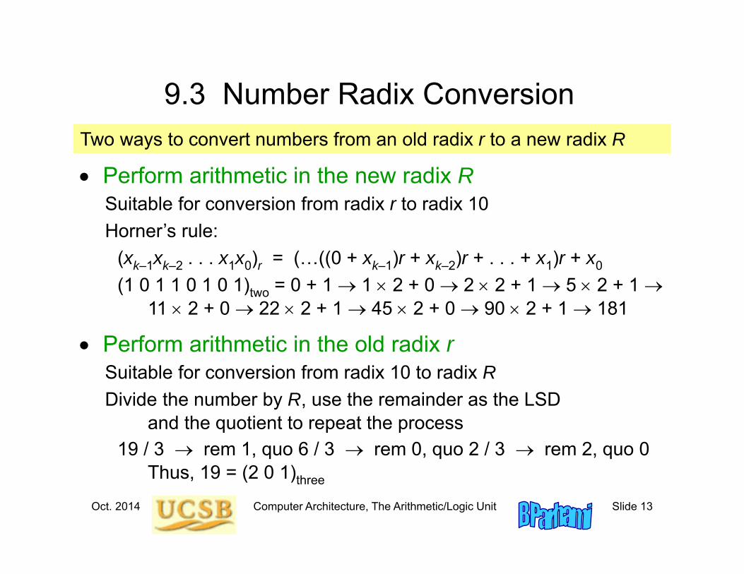
9.3 Number Radix Conversion
Perform arithmetic in the new radix RSuitable for conversion from radix r to radix 10Horner’s rule:
(xk–1xk–2 . . . x1x0)r = (…((0 + xk–1)r + xk–2)r + . . . + x1)r + x0
(1 0 1 1 0 1 0 1)two = 0 + 1 1 2 + 0 2 2 + 1 5 2 + 1 11 2 + 0 22 2 + 1 45 2 + 0 90 2 + 1 181
Perform arithmetic in the old radix rSuitable for conversion from radix 10 to radix RDivide the number by R, use the remainder as the LSD
and the quotient to repeat the process19 / 3 rem 1, quo 6 / 3 rem 0, quo 2 / 3 rem 2, quo 0
Thus, 19 = (2 0 1)three
Two ways to convert numbers from an old radix r to a new radix R
Oct. 2014 Computer Architecture, The Arithmetic/Logic Unit Slide 14
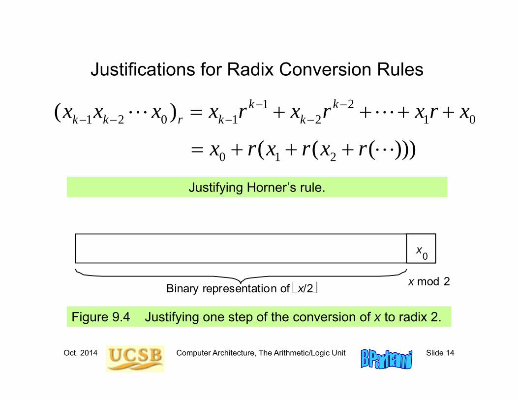
Justifications for Radix Conversion Rules
Figure 9.4 Justifying one step of the conversion of x to radix 2.
x 0
x mod 2 Binary representation of x/2
Justifying Horner’s rule.
1 21 2 0 1 2 1 0( ) k k
k k r k kx x x x r x r x r x
0 1 2( ( ( )))x r x r x r

Oct. 2014 Computer Architecture, The Arithmetic/Logic Unit Slide 15
9.4 Signed Integers
We dealt with representing the natural numbers
Signed or directed whole numbers = integers{ . . . , 3, 2, 1, 0, 1, 2, 3, . . . }
Signed-magnitude representation+27 in 8-bit signed-magnitude binary code 0 0011011–27 in 8-bit signed-magnitude binary code 1 0011011–27 in 2-digit decimal code with BCD digits 1 0010 0111
Biased representationRepresent the interval of numbers [N, P] by the unsigned
interval [0, P + N]; i.e., by adding N to every number
Oct. 2014 Computer Architecture, The Arithmetic/Logic Unit Slide 16
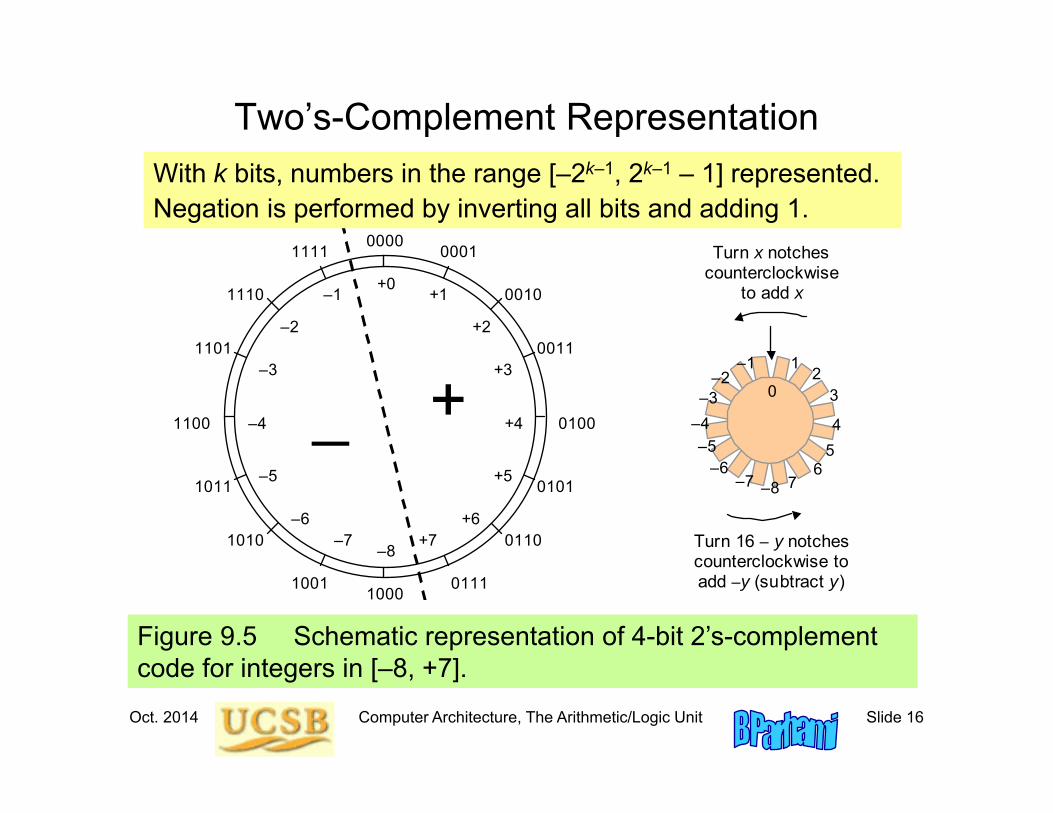
Two’s-Complement Representation
Figure 9.5 Schematic representation of 4-bit 2’s-complement code for integers in [–8, +7].
0000 0001 1111
0010 1110
0011 1101
0100 1100
1000
0101 1011
0110 1010
0111 1001
+0 +1
+2
+3
+4
+5
+6 +7
–1
–5
–2
–3
–4
–8 –7
–6
+ _ 0
1 2
3
–1
4 5
6 7
–8
–7
Turn x notches counterclockwise
to add x
Turn 16 – y notches counterclockwise to add –y (subtract y)
–5
–2 –3
–4
–6
With k bits, numbers in the range [–2k–1, 2k–1 – 1] represented.Negation is performed by inverting all bits and adding 1.
Oct. 2014 Computer Architecture, The Arithmetic/Logic Unit Slide 17
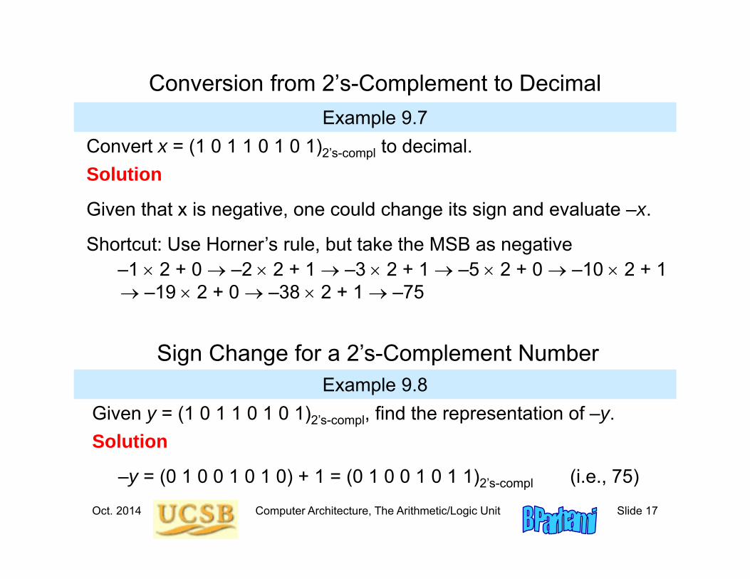
Conversion from 2’s-Complement to DecimalExample 9.7
Convert x = (1 0 1 1 0 1 0 1)2’s-compl to decimal.Solution
Given that x is negative, one could change its sign and evaluate –x.
Shortcut: Use Horner’s rule, but take the MSB as negative–1 2 + 0 –2 2 + 1 –3 2 + 1 –5 2 + 0 –10 2 + 1 –19 2 + 0 –38 2 + 1 –75
Example 9.8Sign Change for a 2’s-Complement Number
Given y = (1 0 1 1 0 1 0 1)2’s-compl, find the representation of –y.Solution
–y = (0 1 0 0 1 0 1 0) + 1 = (0 1 0 0 1 0 1 1)2’s-compl (i.e., 75)
Oct. 2014 Computer Architecture, The Arithmetic/Logic Unit Slide 18
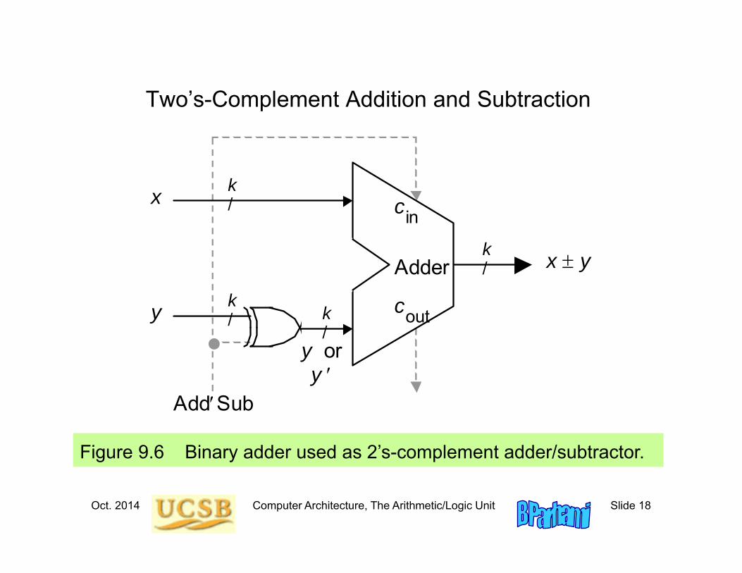
Two’s-Complement Addition and Subtraction
Figure 9.6 Binary adder used as 2’s-complement adder/subtractor.
AddSub
x y
y
x
k /
k /
k /
y or y
Adder
c out
c in
k /
Oct. 2014 Computer Architecture, The Arithmetic/Logic Unit Slide 19
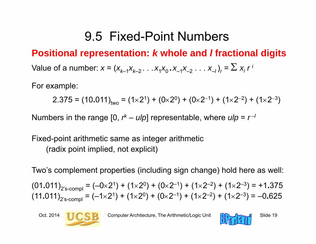
9.5 Fixed-Point NumbersPositional representation: k whole and l fractional digitsValue of a number: x = (xk–1xk–2 . . .x1x0 .x–1x–2 . . . x–l )r = xi r i
For example:
2.375 = (10.011)two = (121) + (020) + (021) + (122) + (123)
Numbers in the range [0, rk – ulp] representable, where ulp = r –l
Fixed-point arithmetic same as integer arithmetic (radix point implied, not explicit)
Two’s complement properties (including sign change) hold here as well:
(01.011)2’s-compl = (–021) + (120) + (02–1) + (12–2) + (12–3) = +1.375(11.011)2’s-compl = (–121) + (120) + (02–1) + (12–2) + (12–3) = –0.625
Oct. 2014 Computer Architecture, The Arithmetic/Logic Unit Slide 20
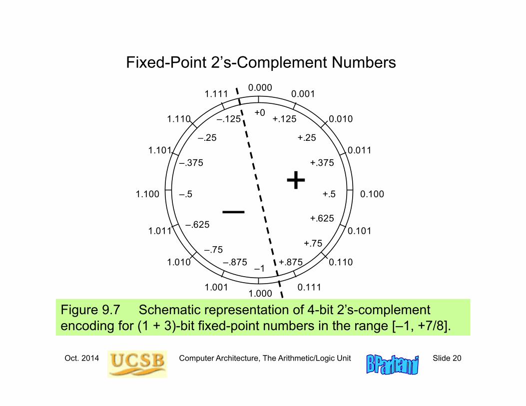
Fixed-Point 2’s-Complement Numbers
Figure 9.7 Schematic representation of 4-bit 2’s-complement encoding for (1 + 3)-bit fixed-point numbers in the range [–1, +7/8].
0.0000.001 1.111
0.010 1.110
0.011 1.101
0.100 1.100
1.000
0.101 1.011
0.110 1.010
0.111 1.001
+0 +.125
+.25
+.375
+.5
+.625
+.75
+.875
–.125
–.625
–.25
–.375
–.5
–1 –.875
–.75
+ _
Oct. 2014 Computer Architecture, The Arithmetic/Logic Unit Slide 21
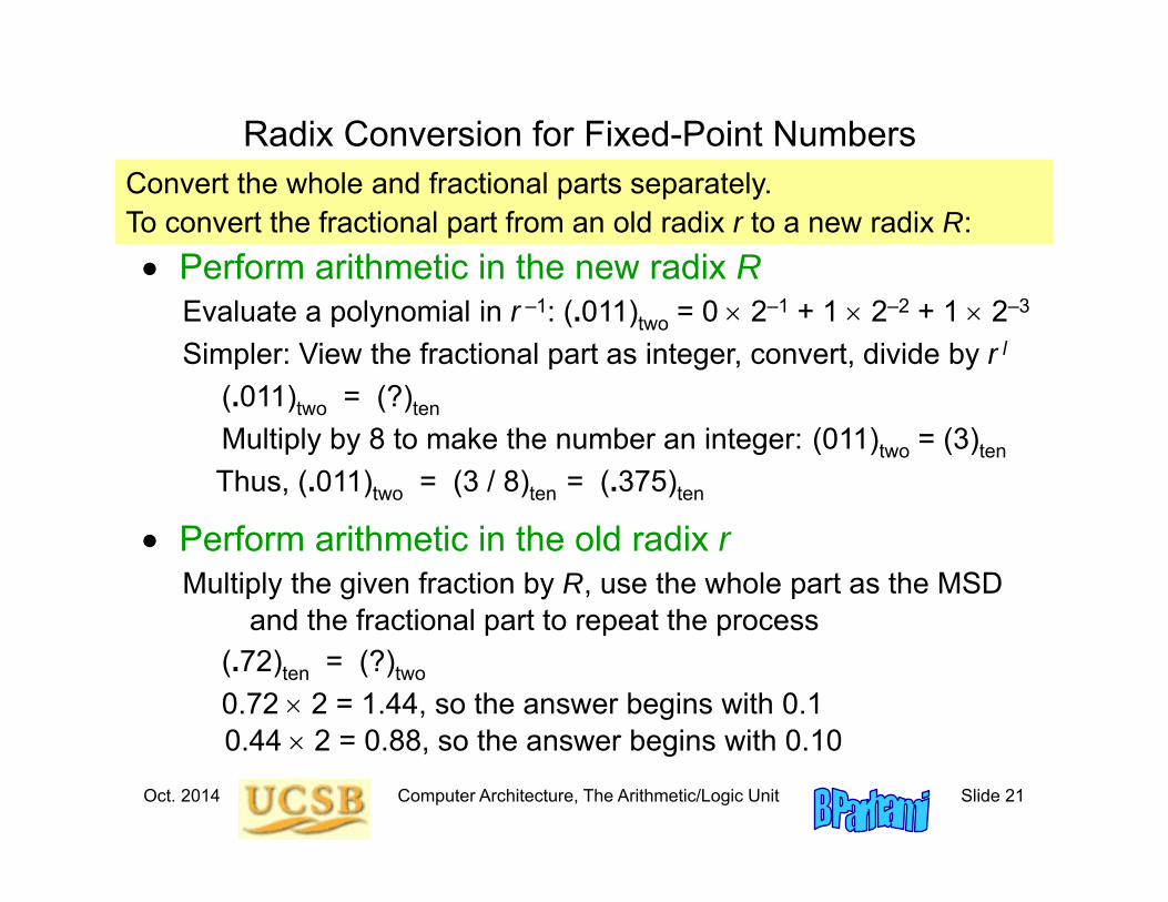
Radix Conversion for Fixed-Point Numbers
Perform arithmetic in the new radix REvaluate a polynomial in r –1: (.011)two = 0 2–1 + 1 2–2 + 1 2–3
Simpler: View the fractional part as integer, convert, divide by r l
(.011)two = (?)ten
Multiply by 8 to make the number an integer: (011)two = (3)ten
Thus, (.011)two = (3 / 8)ten = (.375)ten
Perform arithmetic in the old radix rMultiply the given fraction by R, use the whole part as the MSD
and the fractional part to repeat the process(.72)ten = (?)two
0.72 2 = 1.44, so the answer begins with 0.10.44 2 = 0.88, so the answer begins with 0.10
Convert the whole and fractional parts separately.To convert the fractional part from an old radix r to a new radix R:
Oct. 2014 Computer Architecture, The Arithmetic/Logic Unit Slide 22
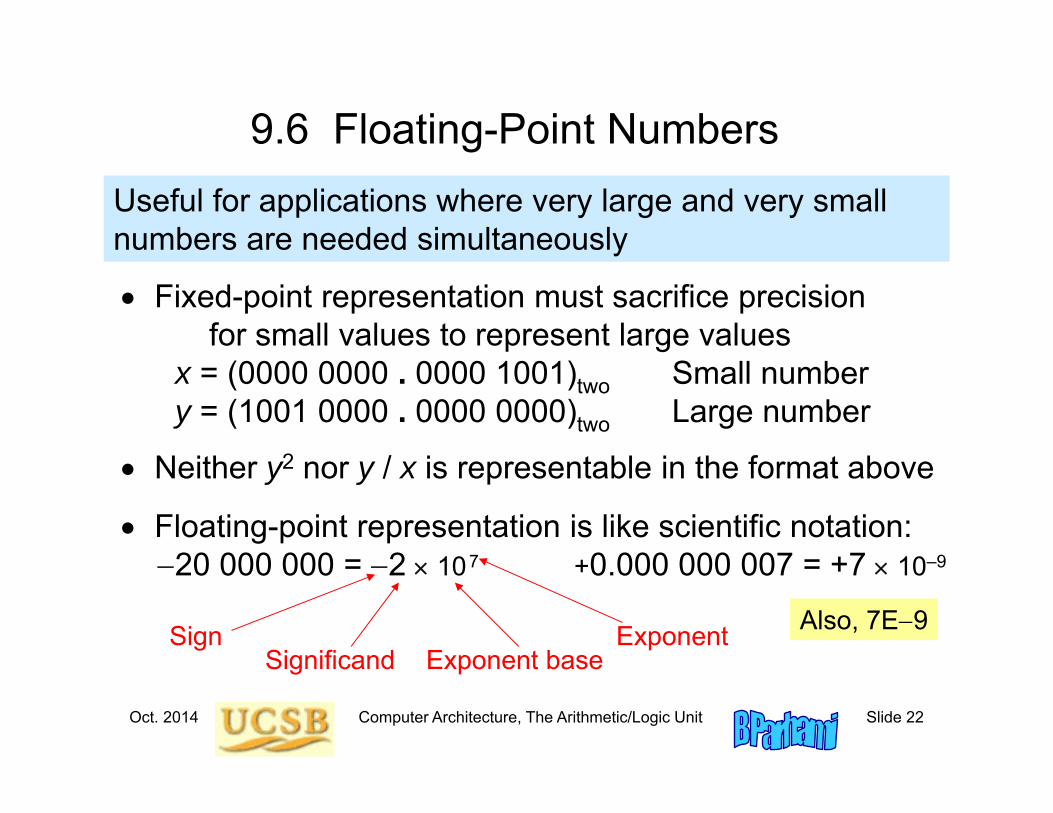
9.6 Floating-Point Numbers
Fixed-point representation must sacrifice precision for small values to represent large values
x = (0000 0000 . 0000 1001)two Small numbery = (1001 0000 . 0000 0000)two Large number
Neither y2 nor y / x is representable in the format above
Floating-point representation is like scientific notation: 20 000 000 = 2 107 +0.000 000 007 = +7 10–9
Useful for applications where very large and very small numbers are needed simultaneously
Also, 7E9Significand
ExponentExponent base
Sign
Oct. 2014 Computer Architecture, The Arithmetic/Logic Unit Slide 23
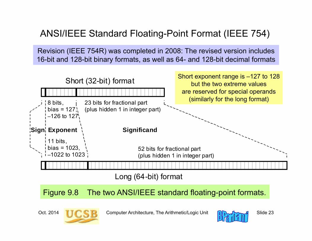
ANSI/IEEE Standard Floating-Point Format (IEEE 754)
Figure 9.8 The two ANSI/IEEE standard floating-point formats.
Short (32-bit) format
Long (64-bit) format
Sign Exponent Significand
8 bits, bias = 127, –126 to 127
11 bits, bias = 1023, –1022 to 1023
52 bits for fractional part (plus hidden 1 in integer part)
23 bits for fractional part (plus hidden 1 in integer part)
Short exponent range is –127 to 128but the two extreme values
are reserved for special operands(similarly for the long format)
Revision (IEEE 754R) was completed in 2008: The revised version includes 16-bit and 128-bit binary formats, as well as 64- and 128-bit decimal formats
Oct. 2014 Computer Architecture, The Arithmetic/Logic Unit Slide 24
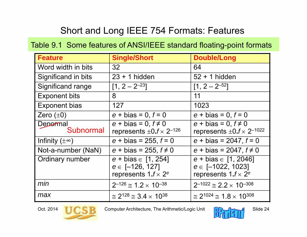
Short and Long IEEE 754 Formats: FeaturesTable 9.1 Some features of ANSI/IEEE standard floating-point formats
Feature Single/Short Double/LongWord width in bits 32 64Significand in bits 23 + 1 hidden 52 + 1 hiddenSignificand range [1, 2 – 2–23] [1, 2 – 2–52]Exponent bits 8 11Exponent bias 127 1023Zero (±0) e + bias = 0, f = 0 e + bias = 0, f = 0Denormal e + bias = 0, f ≠ 0
represents ±0.f 2–126e + bias = 0, f ≠ 0represents ±0.f 2–1022
Infinity (∞) e + bias = 255, f = 0 e + bias = 2047, f = 0Not-a-number (NaN) e + bias = 255, f ≠ 0 e + bias = 2047, f ≠ 0Ordinary number e + bias [1, 254]
e [–126, 127]represents 1.f 2e
e + bias [1, 2046]e [–1022, 1023]represents 1.f 2e
min 2–126 1.2 10–38 2–1022 2.2 10–308
max 2128 3.4 1038 21024 1.8 10308
Subnormal
Oct. 2014 Computer Architecture, The Arithmetic/Logic Unit Slide 25
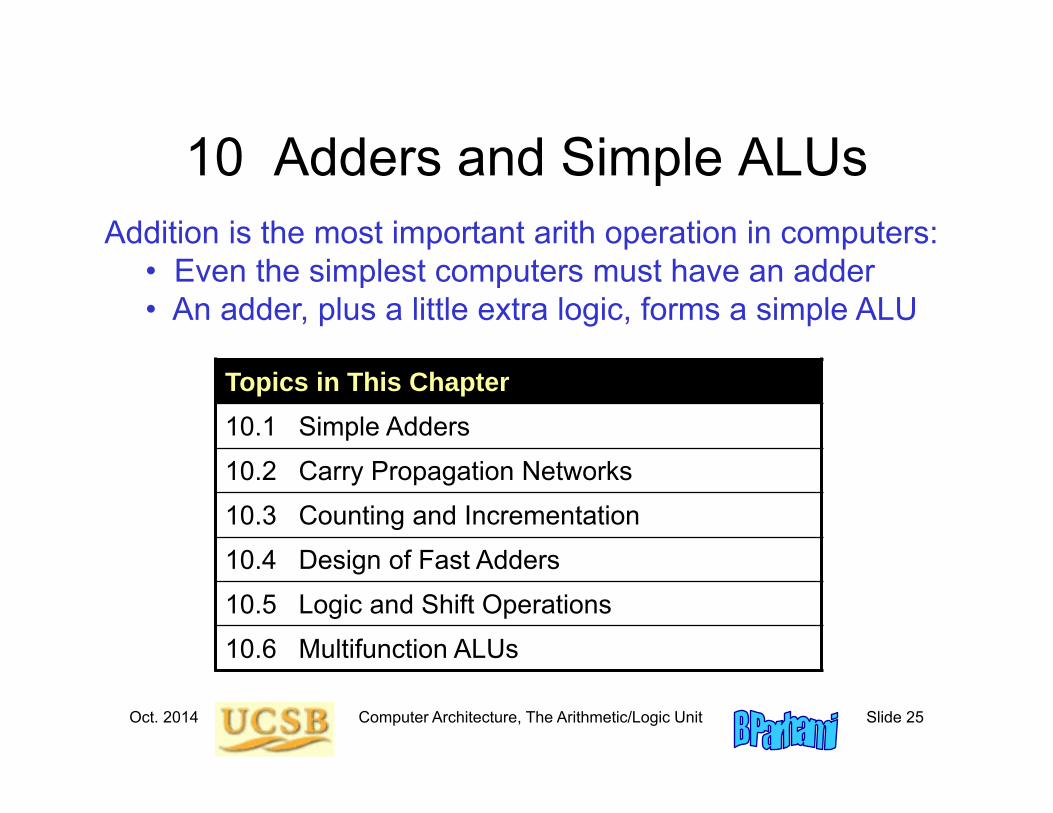
10 Adders and Simple ALUsAddition is the most important arith operation in computers:
• Even the simplest computers must have an adder• An adder, plus a little extra logic, forms a simple ALU
Topics in This Chapter10.1 Simple Adders
10.2 Carry Propagation Networks
10.3 Counting and Incrementation
10.4 Design of Fast Adders
10.5 Logic and Shift Operations
10.6 Multifunction ALUs
Oct. 2014 Computer Architecture, The Arithmetic/Logic Unit Slide 26
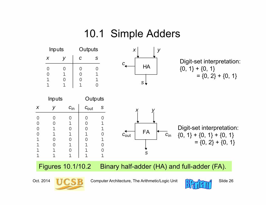
10.1 Simple Adders
Figures 10.1/10.2 Binary half-adder (HA) and full-adder (FA).
x y c s 0 0 0 0 0 1 0 1 1 0 0 1 1 1 1 0
Inputs Outputs
HA
x y
c
s
x y c c s 0 0 0 0 0 0 0 1 0 1 0 1 0 0 1 0 1 1 1 0 1 0 0 0 1 1 0 1 1 0 1 1 0 1 0 1 1 1 1 1
Inputs Outputs
c out c in
out in x
y
s
FA
Digit-set interpretation:{0, 1} + {0, 1}
= {0, 2} + {0, 1}
Digit-set interpretation:{0, 1} + {0, 1} + {0, 1}
= {0, 2} + {0, 1}
Oct. 2014 Computer Architecture, The Arithmetic/Logic Unit Slide 27
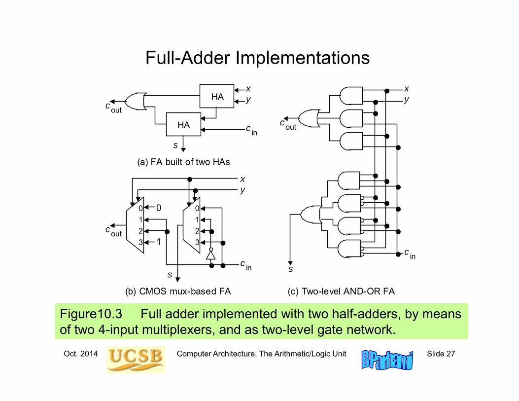
Full-Adder Implementations
Figure10.3 Full adder implemented with two half-adders, by means of two 4-input multiplexers, and as two-level gate network.
(a) FA built of two HAs
(c) Two-level AND-OR FA (b) CMOS mux-based FA
1
0
3
2
HA
HA
1
0
3
2
0
1
x y
x y
x y
s
s s
c out
c out
c out
c in
c in
c in
Oct. 2014 Computer Architecture, The Arithmetic/Logic Unit Slide 28
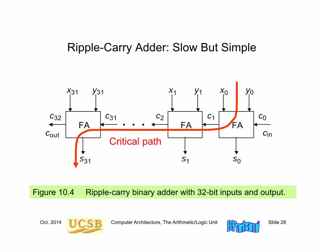
Ripple-Carry Adder: Slow But Simple
Figure 10.4 Ripple-carry binary adder with 32-bit inputs and output.
x
s
y
c c
x
s
y
c
x
s
y
c
c out c in
0 0
0
c 0
1 1
1
1 2
31
31
31
31
FA FA FA 32 . . .
Critical path
Oct. 2014 Computer Architecture, The Arithmetic/Logic Unit Slide 29
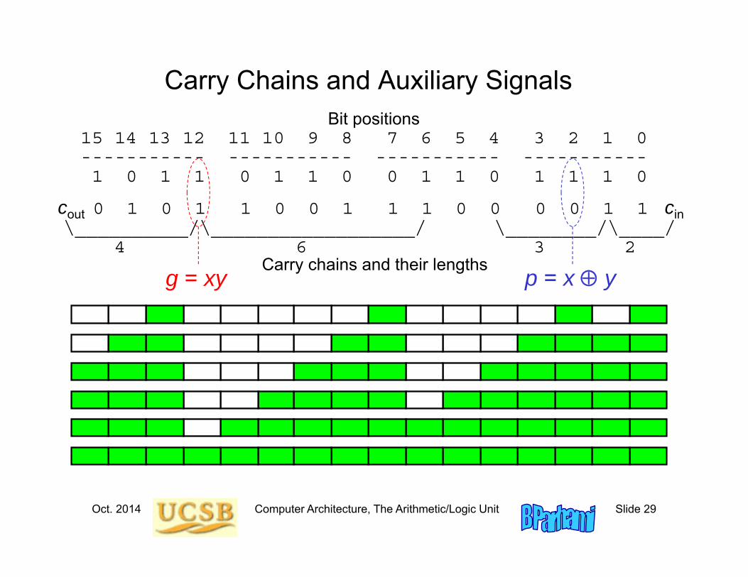
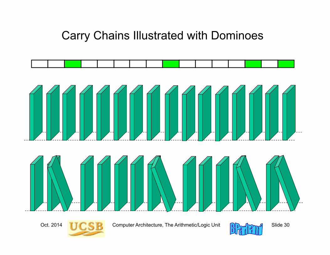
Carry Chains and Auxiliary SignalsBit positions
15 14 13 12 11 10 9 8 7 6 5 4 3 2 1 0----------- ----------- ----------- -----------1 0 1 1 0 1 1 0 0 1 1 0 1 1 1 0
cout 0 1 0 1 1 0 0 1 1 1 0 0 0 0 1 1 cin\__________/\__________________/ \________/\____/
4 6 3 2Carry chains and their lengths
g = xy p = x y
Oct. 2014 Computer Architecture, The Arithmetic/Logic Unit Slide 30
Carry Chains Illustrated with Dominoes
Oct. 2014 Computer Architecture, The Arithmetic/Logic Unit Slide 31
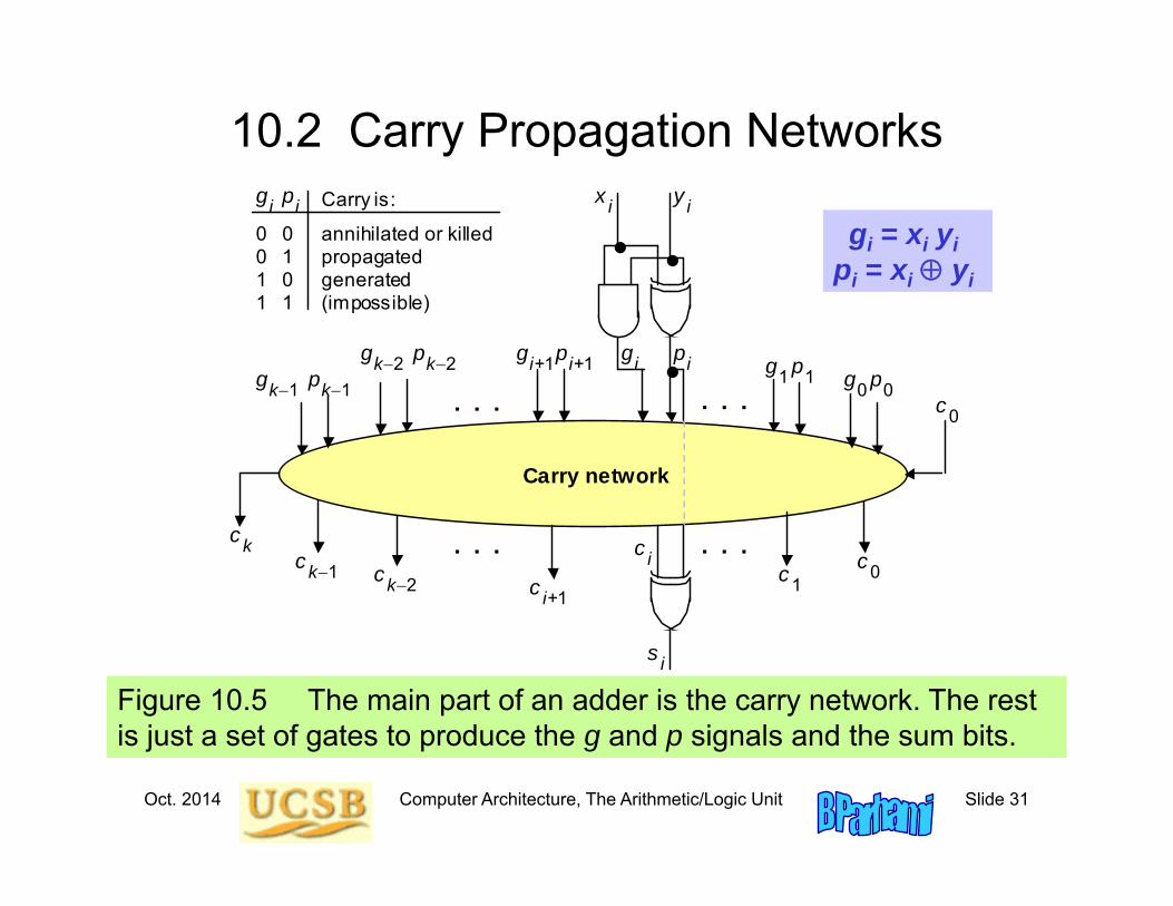
10.2 Carry Propagation Networks
Figure 10.5 The main part of an adder is the carry network. The rest is just a set of gates to produce the g and p signals and the sum bits.
Carry network
. . . . . .
x i y i
g p
s
i i
i
c i c i+1
c k1
c k c k2 c 1
c 0
g p 1 1 g p 0 0
g p k2 k2 g p i+1 i+1 g p k1 k1
c 0 . . . . . .
0 0 0 1 1 0 1 1
annihilated or killed propagated generated (impossible)
Carry is: g i p i gi = xi yi
pi = xi yi

Oct. 2014 Computer Architecture, The Arithmetic/Logic Unit Slide 32
Ripple-Carry Adder Revisited
Figure 10.6 The carry propagation network of a ripple-carry adder.
. . . c
k1
c
k c k2
c 1
g
p
1
1
g
p
0
0
g
p
k2
k2
g
p
k1
k1
c
0 c 2
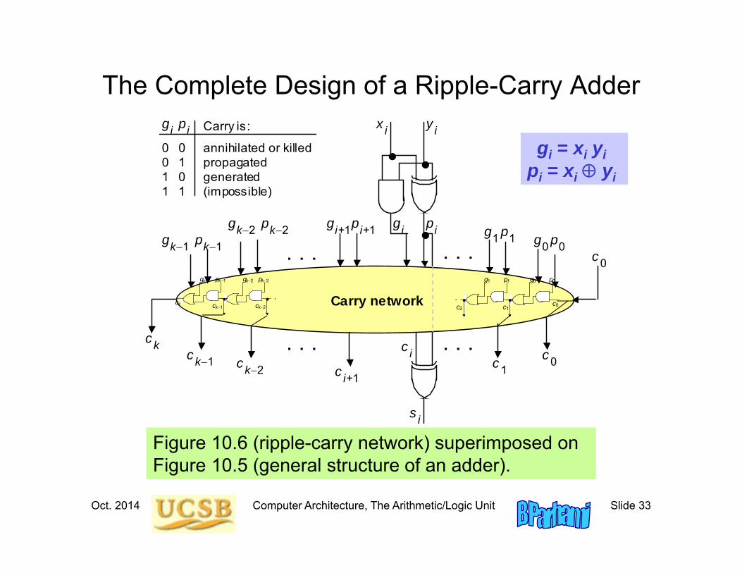
The carry recurrence: ci+1 = gi pi ci
Latency of k-bit adder is roughly 2k gate delays:
1 gate delay for production of p and g signals, plus 2(k – 1) gate delays for carry propagation, plus1 XOR gate delay for generation of the sum bits
Oct. 2014 Computer Architecture, The Arithmetic/Logic Unit Slide 33
The Complete Design of a Ripple-Carry Adder
Figure 10.6 (ripple-carry network) superimposed on Figure 10.5 (general structure of an adder).
Carry network
. . . . . .
x i y i
g p
s
i i
i
c i c i+1
c k1
c k c k2 c 1
c 0
g p 1 1 g p 0 0
g p k2 k2 g p i+1 i+1 g p k1 k1
c 0 . . . . . .
0 0 0 1 1 0 1 1
annihilated or killed propagated generated (impossible)
Carry is: g i p i gi = xi yi
pi = xi yi
. c 1
g
p
1
1
g
p
0
0
c
0 c
2
.c
k1
c
k c k2
g
p
k2
k2
g
p
k1
k1
Oct. 2014 Computer Architecture, The Arithmetic/Logic Unit Slide 34
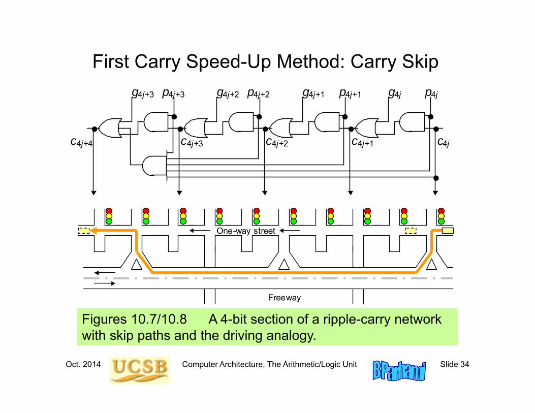
First Carry Speed-Up Method: Carry Skip
Figures 10.7/10.8 A 4-bit section of a ripple-carry network with skip paths and the driving analogy.
c
g
p
4j+1
4j+1
g
p
4j
4j
g
p
4j+2
4j+2
g
p
4j+3
4j+3
c
4j
4j+4
c
4j+3
c
4j+2
c
4j+1
One-way street
Freeway

Oct. 2014 Computer Architecture, The Arithmetic/Logic Unit Slide 35
Mux-Based Skip Carry Logic
The carry-skip adder of Fig. 10.7 works fine if we begin with a clean slate, where all signals are 0s; otherwise, it will run into problems, which do not exist in this mux-based implementation
c
g
p
4j+1
4j+1
g
p
4j
4j
g
p
4j+2
4j+2
g
p
4j+3
4j+3
c
4j
4j+4
c
4j+3
c
4j+2
c
4j+1
01
p[4j, 4j+3]
c4j+4
c
g
p
4j+1
4j+1
g
p
4j
4j
g
p
4j+2
4j+2
g
p
4j+3
4j+3
c
4j
4j+4
c
4j+3
c
4j+2
c
4j+1
Fig. 10.7

Oct. 2014 Computer Architecture, The Arithmetic/Logic Unit Slide 36
10.3 Counting and Incrementation
Figure 10.9 Schematic diagram of an initializable synchronous counter.
D Q
C _ Q
D
c out
c in
Adder
Update
/ k
k /
a (Increment
amount)
Count register k
/ 1
0
Data in
k /
k /
IncrInit
Oct. 2014 Computer Architecture, The Arithmetic/Logic Unit Slide 37
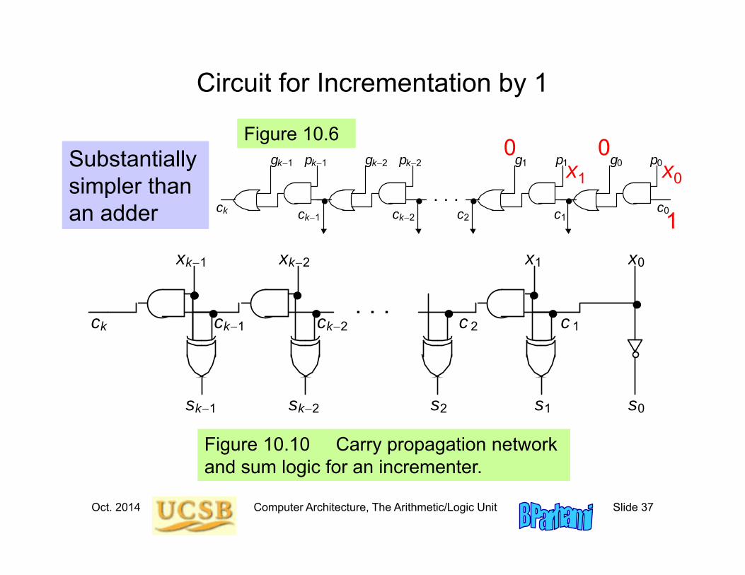
Circuit for Incrementation by 1
Substantially simpler than an adder
Figure 10.10 Carry propagation network and sum logic for an incrementer.
1
0
k2
k1
. . . c
k1
c
k
c
k2
c
1
x
x
x
x
c
2
1 0 k2 k1 s s s s 2 s
. . . c k1
c
k c k2
c 1
g
p
1
1
g
p
0
0
g
p
k2
k2
g
p
k1
k1
c
0 c
2
00x0x1
Figure 10.6
1
Oct. 2014 Computer Architecture, The Arithmetic/Logic Unit Slide 38
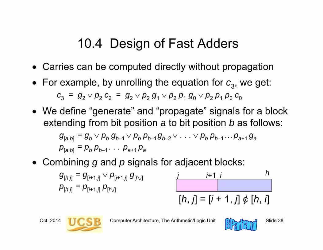
Carries can be computed directly without propagation For example, by unrolling the equation for c3, we get:
c3 = g2 p2 c2 = g2 p2 g1 p2 p1 g0 p2 p1 p0 c0
We define “generate” and “propagate” signals for a block extending from bit position a to bit position b as follows:
g[a,b] = gb pb gb–1 pb pb–1gb–2 . . . pb pb–1…pa+1 ga
p[a,b] = pb pb–1. . . pa+1 pa
Combining g and p signals for adjacent blocks:g[h,j] = g[i+1,j] p[i+1,j] g[h,i]
p[h,j] = p[i+1,j] p[h,i]
10.4 Design of Fast Adders
hii+1j
[h, j] = [i + 1, j] ¢ [h, i]
Oct. 2014 Computer Architecture, The Arithmetic/Logic Unit Slide 39
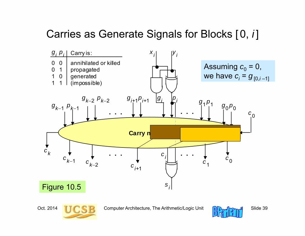
Carries as Generate Signals for Blocks [ 0, i ]
Figure 10.5
Carry network
. . . . . .
x i y i
g p
s
i i
i
c i c i+1
c k1
c k c k2 c 1
c 0
g p 1 1 g p 0 0
g p k2 k2 g p i+1 i+1 g p k1 k1
c 0 . . . . . .
0 0 0 1 1 0 1 1
annihilated or killed propagated generated (impossible)
Carry is: g i p i
Assuming c0 = 0, we have ci = g [0,i –1]
Oct. 2014 Computer Architecture, The Arithmetic/Logic Unit Slide 40
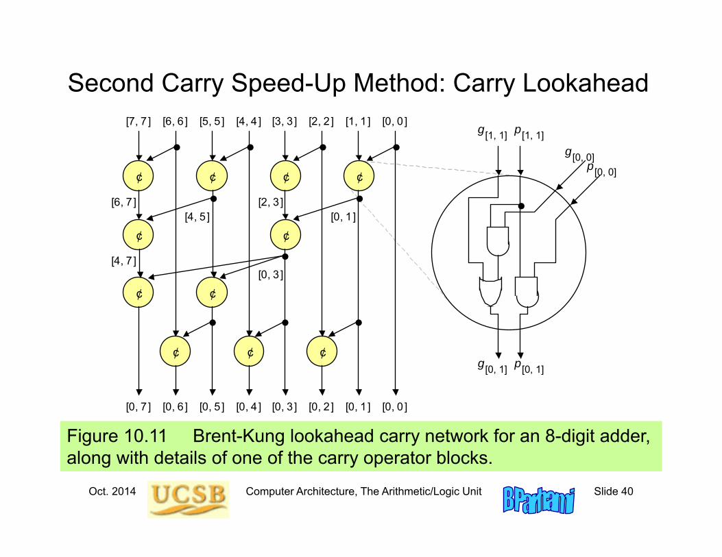
Second Carry Speed-Up Method: Carry Lookahead
Figure 10.11 Brent-Kung lookahead carry network for an 8-digit adder, along with details of one of the carry operator blocks.
¢ ¢ ¢ ¢
¢ ¢
¢ ¢
¢ ¢ ¢
[7, 7 ] [6, 6 ] [5, 5 ] [4, 4 ] [3, 3 ] [2, 2 ] [1, 1 ] [0, 0 ]
[0, 7 ] [0, 6 ] [0, 5 ] [0, 4 ] [0, 3 ] [0, 2 ] [0, 1 ] [0, 0 ]
[2, 3 ] [4, 5 ]
[6, 7 ]
[4, 7 ] [0, 3 ]
[0, 1 ]
g [0, 0]
g [0, 1]
g [1, 1]
p [0, 0]
p [0, 1]
p [1, 1]
Oct. 2014 Computer Architecture, The Arithmetic/Logic Unit Slide 41
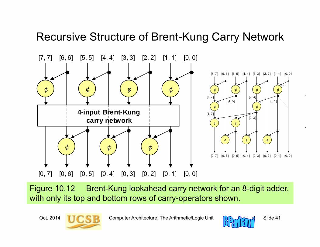
Recursive Structure of Brent-Kung Carry Network
Figure 10.12 Brent-Kung lookahead carry network for an 8-digit adder, with only its top and bottom rows of carry-operators shown.
¢ ¢ ¢ ¢
¢ ¢ ¢
[7, 7] [6, 6] [5, 5] [4, 4] [3, 3] [2, 2] [1, 1] [0, 0]
[0, 7] [0, 6] [0, 5] [0, 4] [0, 3] [0, 2] [0, 1] [0, 0]
4-input Brent-Kung carry network
¢ ¢ ¢ ¢
¢ ¢
¢ ¢
¢ ¢ ¢
[7, 7 ] [6, 6 ] [5, 5 ] [4, 4 ] [3, 3 ] [2, 2 ] [1, 1 ] [0, 0 ]
[0, 7 ] [0, 6 ] [0, 5 ] [0, 4 ] [0, 3 ] [0, 2 ] [0, 1 ] [0, 0 ]
[2, 3 ] [4, 5 ]
[6, 7 ]
[4, 7 ] [0, 3 ]
[0, 1 ]
Oct. 2014 Computer Architecture, The Arithmetic/Logic Unit Slide 42
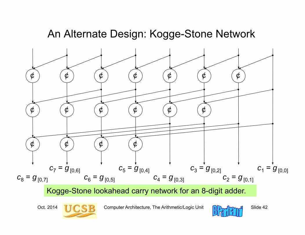
An Alternate Design: Kogge-Stone Network
Kogge-Stone lookahead carry network for an 8-digit adder.
¢ ¢ ¢ ¢
¢ ¢ ¢ ¢
¢ ¢
¢ ¢¢ ¢
¢
¢ ¢
c1 = g [0,0]c2 = g [0,1]
c3 = g [0,2]c8 = g [0,7] c4 = g [0,3]
c5 = g [0,4]c6 = g [0,5]
c7 = g [0,6]
Oct. 2014 Computer Architecture, The Arithmetic/Logic Unit Slide 43
¢ ¢ ¢ ¢
¢ ¢
¢ ¢
¢ ¢ ¢
[7, 7 ] [6, 6 ] [5, 5 ] [4, 4 ] [3, 3 ] [2, 2 ] [1, 1 ] [0, 0 ]
[0, 7 ] [0, 6 ] [0, 5 ] [0, 4 ] [0, 3 ] [0, 2 ] [0, 1 ] [0, 0 ]
[2, 3 ] [4, 5 ]
[6, 7 ]
[4, 7 ] [0, 3 ]
[0, 1 ]
g [0, 0]
g [0, 1]
g [1, 1]
p [0, 0]
p [0, 1]
p [1, 1]
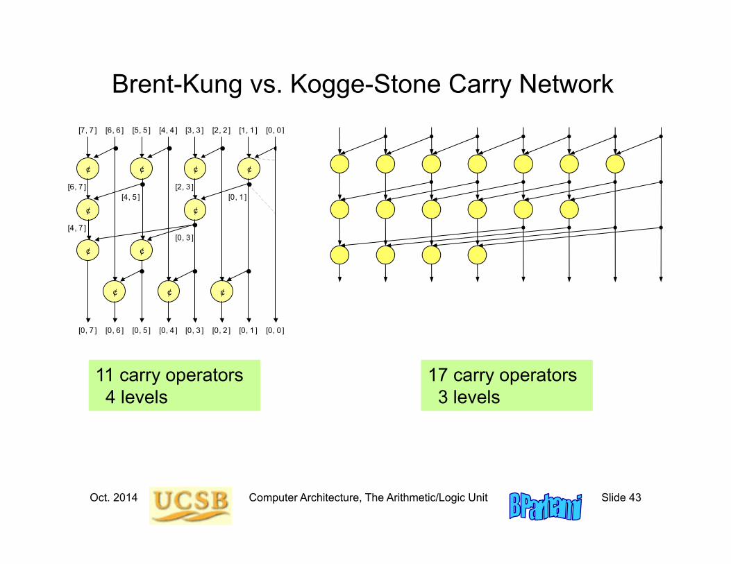
Brent-Kung vs. Kogge-Stone Carry Network
11 carry operators4 levels
17 carry operators3 levels
Oct. 2014 Computer Architecture, The Arithmetic/Logic Unit Slide 44
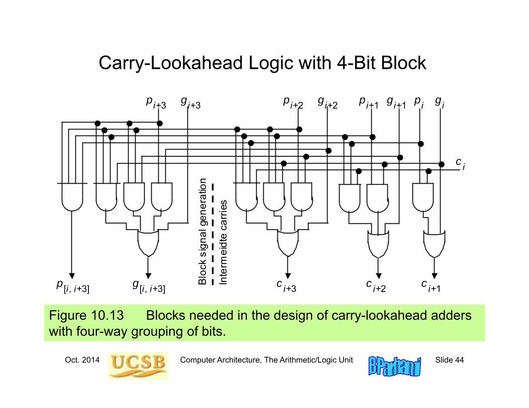
Carry-Lookahead Logic with 4-Bit Block
Figure 10.13 Blocks needed in the design of carry-lookahead adders with four-way grouping of bits.
Bloc
k si
gnal
gen
erat
ion
p [i, i+3]
c i
Inte
rmei
dte
carr
ies
c i+1 c i+2 c i+3 g [i, i+3]
p i+3 g i+3 p i+2 g i+2 p i+1 g i+1 p i g i
Oct. 2014 Computer Architecture, The Arithmetic/Logic Unit Slide 45
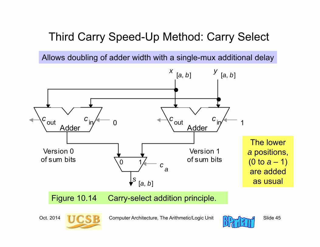
Third Carry Speed-Up Method: Carry Select
Figure 10.14 Carry-select addition principle.
c out c in Adder
Version 1 of sum bits 1
0
x [a, b]
c out c in Adder
Version 0 of sum bits
y [a, b]
s [a, b]
c a
0 1
Allows doubling of adder width with a single-mux additional delay
The lowera positions, (0 to a – 1) are added as usual
Oct. 2014 Computer Architecture, The Arithmetic/Logic Unit Slide 46
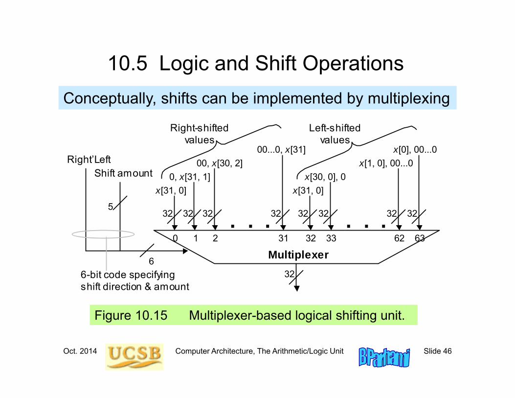
10.5 Logic and Shift OperationsConceptually, shifts can be implemented by multiplexing
Figure 10.15 Multiplexer-based logical shifting unit.
Multiplexer
0 1 2 31 32 33 62 63
5
6
Right’Left Shift amount 0, x[31, 1]
x[31, 0]
00, x[30, 2] 00...0, x[31]
x[31, 0] x[30, 0], 0
x[1, 0], 00...0 x[0], 00...0
. . . . . .
32
32 32 32 32 32 32 32 32
6-bit code specifying shift direction & amount
Right-shifted values
Left-shifted values
Oct. 2014 Computer Architecture, The Arithmetic/Logic Unit Slide 47
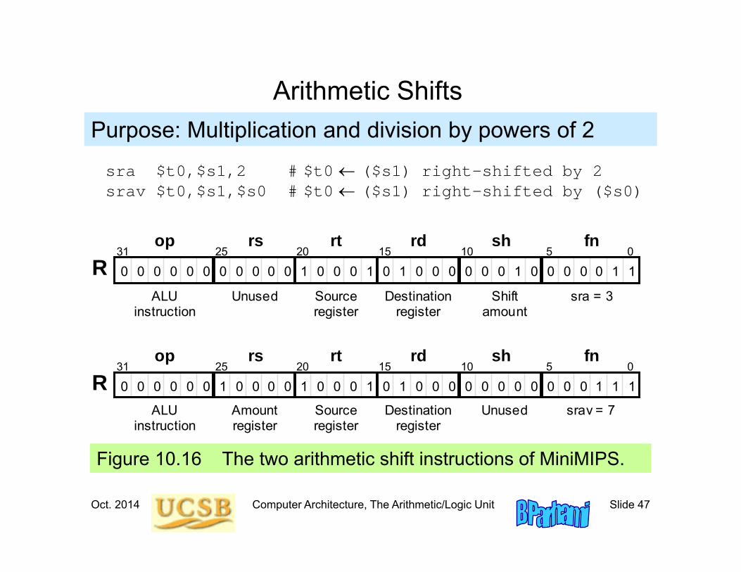
Arithmetic Shifts
Figure 10.16 The two arithmetic shift instructions of MiniMIPS.
Purpose: Multiplication and division by powers of 2
sra $t0,$s1,2 # $t0 ($s1) right-shifted by 2srav $t0,$s1,$s0 # $t0 ($s1) right-shifted by ($s0)
1 1
1 1
0 0 0
fn
0 0 0 0 0 0 0 0 0 0 0 1 0 0 0 0 1 1 1 0 0 0 0 0 0 0 0 31 25 20 15 0
ALU instruction
Unused Source register
op rs rt
R rd sh
10 5
Destination register
Shift amount
sra = 3
1 0 0 0 0 0 0 0 0 0 0 0 0 0 0 0 0 0 1 1 1 1 0 0 0 0 0 0 0 0 31 25 20 15 0
ALU instruction
Amount register
Source register
op rs rt
R rd sh
10 5 fn
Destination register
Unused srav = 7
Oct. 2014 Computer Architecture, The Arithmetic/Logic Unit Slide 48
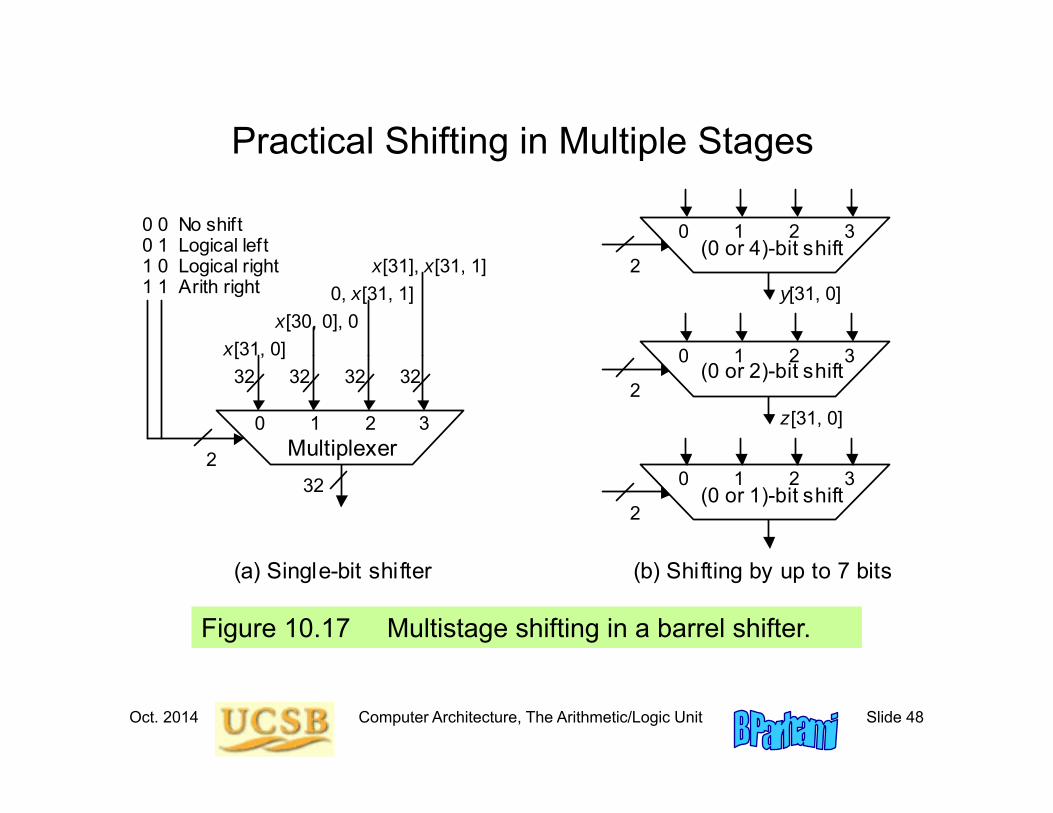
Practical Shifting in Multiple Stages
Figure 10.17 Multistage shifting in a barrel shifter.
2
0, x[31, 1]
x[31, 0] x[30, 0], 0
32
0 1 2 3
32 32 32 32
0 0 No shift 0 1 Logical left 1 0 Logical right 1 1 Arith right
x[31], x[31, 1]
Multiplexer
2
0 1 2 3 (0 or 4)-bit shift
2
0 1 2 3 (0 or 2)-bit shift
2
0 1 2 3 (0 or 1)-bit shift
(a) Single-bit shifter (b) Shifting by up to 7 bits
y[31, 0]
z[31, 0]
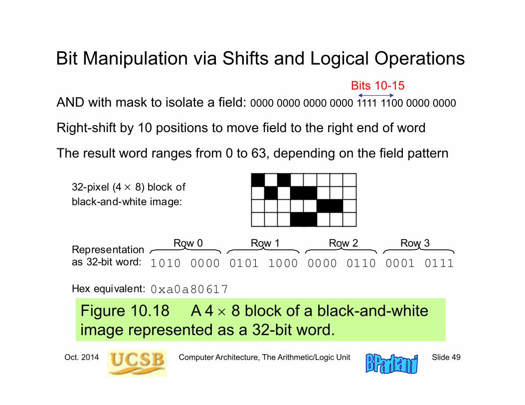
Oct. 2014 Computer Architecture, The Arithmetic/Logic Unit Slide 49
Figure 10.18 A 4 8 block of a black-and-white image represented as a 32-bit word.
Bit Manipulation via Shifts and Logical Operations
AND with mask to isolate a field: 0000 0000 0000 0000 1111 1100 0000 0000
Right-shift by 10 positions to move field to the right end of word
The result word ranges from 0 to 63, depending on the field pattern
32-pixel (4 8) block of black-and-white image:
1010 0000 0101 1000 0000 0110 0001 0111 Representation as 32-bit word:
Hex equivalent: 0xa0a80617
Row 0 Row 1 Row 2 Row 3
Bits 10-15
Oct. 2014 Computer Architecture, The Arithmetic/Logic Unit Slide 50
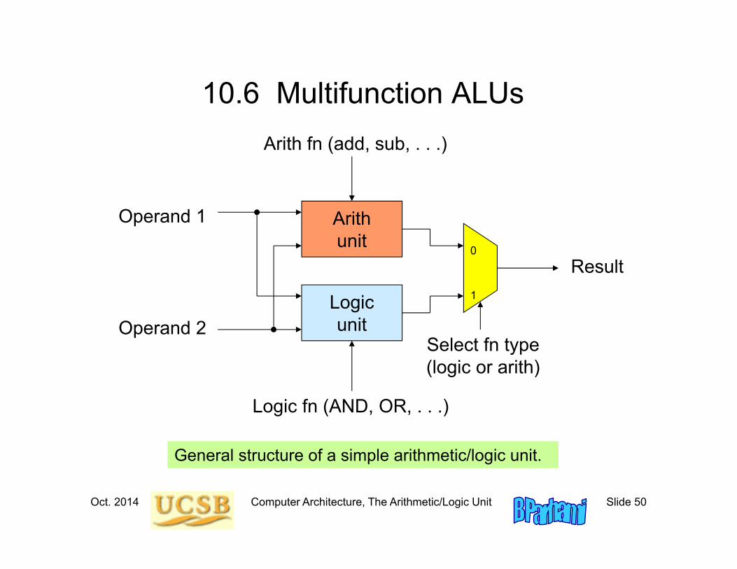
10.6 Multifunction ALUs
General structure of a simple arithmetic/logic unit.
Logicunit
Arithunit 0
1
Operand 1
Operand 2
Result
Logic fn (AND, OR, . . .)
Arith fn (add, sub, . . .)
Select fn type (logic or arith)
Oct. 2014 Computer Architecture, The Arithmetic/Logic Unit Slide 51
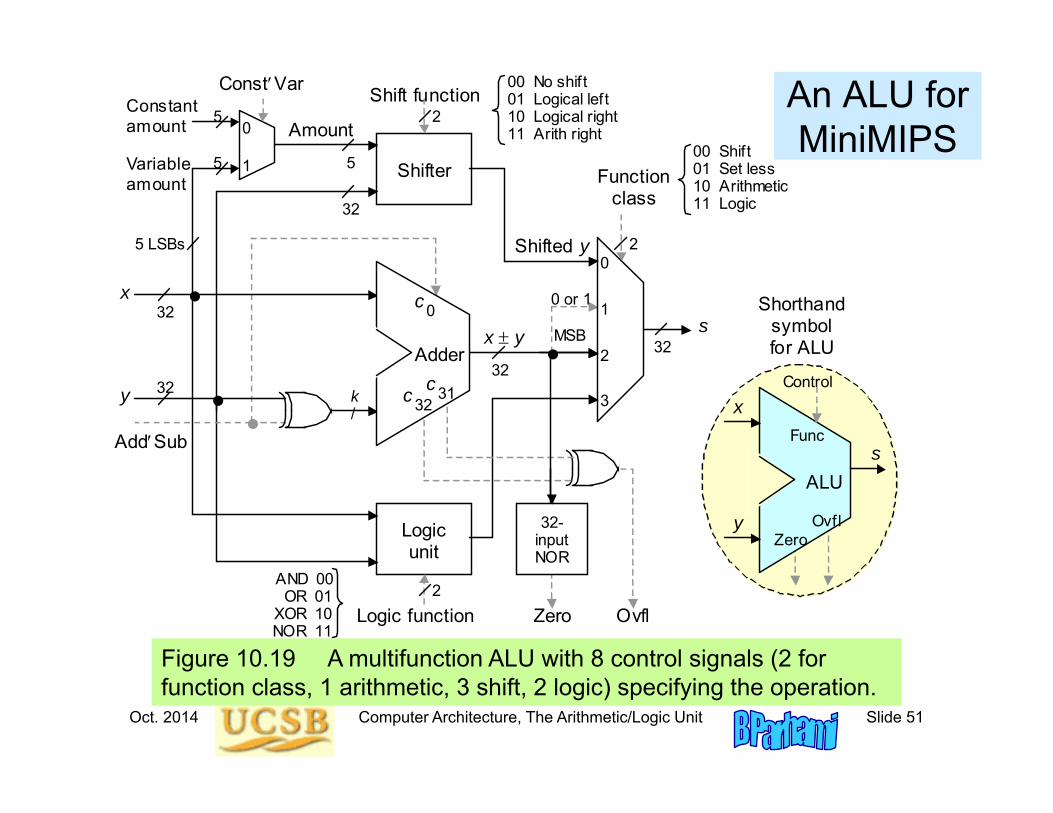
An ALU for MiniMIPS
Figure 10.19 A multifunction ALU with 8 control signals (2 for function class, 1 arithmetic, 3 shift, 2 logic) specifying the operation.
AddSub
x y
y
x
Adder
c 32
c 0
k /
Shifter
Logic unit
s
Logic function
Amount
5
2
Constant amount
Variable amount
5
5
ConstVar
0
1
0
1
2
3
Function class
2
Shift function
5 LSBs Shifted y
32
32
32
2
c 31
32-input NOR
Ovfl Zero
32 32
MSB
ALU
y
x
s
Shorthand symbol for ALU
Ovfl Zero
Func
Control
0 or 1
AND 00 OR 01
XOR 10 NOR 11
00 Shift 01 Set less 10 Arithmetic 11 Logic
00 No shift 01 Logical left 10 Logical right 11 Arith right

Oct. 2014 Computer Architecture, The Arithmetic/Logic Unit Slide 52
11 Multipliers and DividersModern processors perform many multiplications & divisions:
• Encryption, image compression, graphic rendering• Hardware vs programmed shift-add/sub algorithms
Topics in This Chapter
11.1 Shift-Add Multiplication
11.2 Hardware Multipliers
11.3 Programmed Multiplication
11.4 Shift-Subtract Division
11.5 Hardware Dividers
11.6 Programmed Division
Oct. 2014 Computer Architecture, The Arithmetic/Logic Unit Slide 53
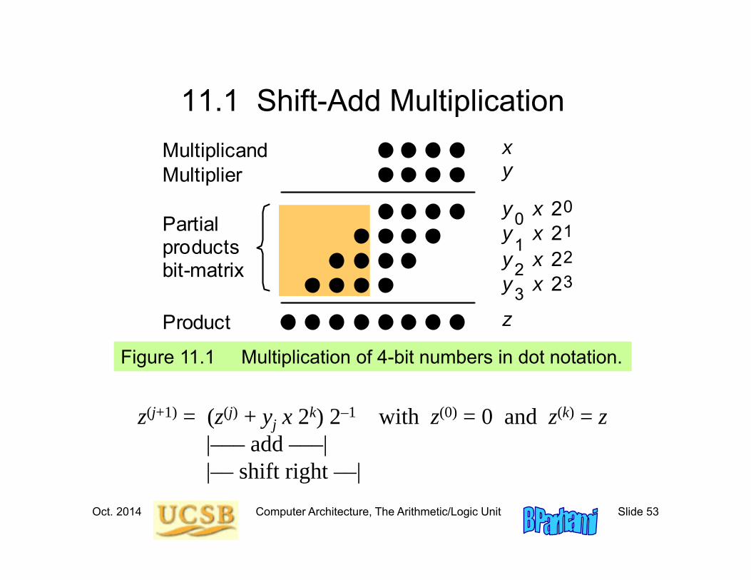
11.1 Shift-Add Multiplication
Figure 11.1 Multiplication of 4-bit numbers in dot notation.
Multiplicand
Partial products bit-matrix
x y
z
y x 2 0 0
y x 2 1 1
y x 2 2 2
y x 2 3 3
Multiplier
Product
z(j+1) = (z(j) + yj x 2k) 2–1 with z(0) = 0 and z(k) = z|––– add –––||–– shift right ––|
Oct. 2014 Computer Architecture, The Arithmetic/Logic Unit Slide 54
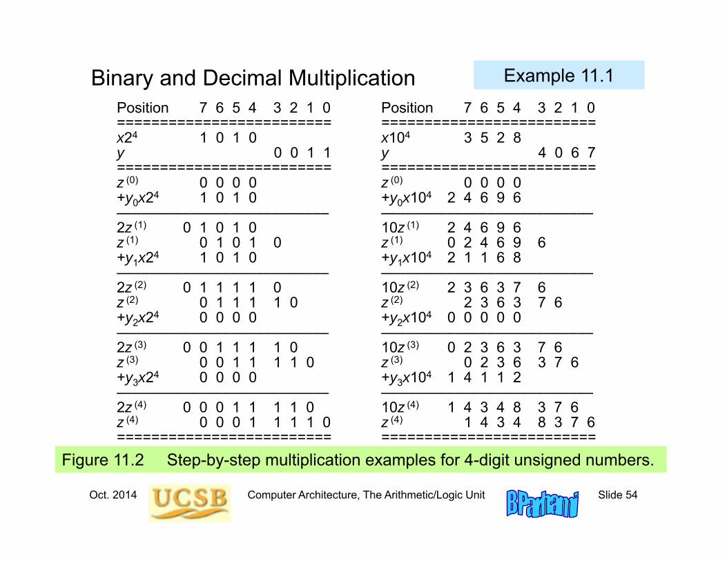
Binary and Decimal Multiplication
Figure 11.2 Step-by-step multiplication examples for 4-digit unsigned numbers.
Position 7 6 5 4 3 2 1 0 Position 7 6 5 4 3 2 1 0========================= =========================x24 1 0 1 0 x104 3 5 2 8y 0 0 1 1 y 4 0 6 7========================= =========================z (0) 0 0 0 0 z (0) 0 0 0 0+y0x24 1 0 1 0 +y0x104 2 4 6 9 6–––––––––––––––––––––––––– ––––––––––––––––––––––––––2z (1) 0 1 0 1 0 10z (1) 2 4 6 9 6z (1) 0 1 0 1 0 z (1) 0 2 4 6 9 6+y1x24 1 0 1 0 +y1x104 2 1 1 6 8–––––––––––––––––––––––––– ––––––––––––––––––––––––––2z (2) 0 1 1 1 1 0 10z (2) 2 3 6 3 7 6z (2) 0 1 1 1 1 0 z (2) 2 3 6 3 7 6+y2x24 0 0 0 0 +y2x104 0 0 0 0 0–––––––––––––––––––––––––– ––––––––––––––––––––––––––2z (3) 0 0 1 1 1 1 0 10z (3) 0 2 3 6 3 7 6z (3) 0 0 1 1 1 1 0 z (3) 0 2 3 6 3 7 6+y3x24 0 0 0 0 +y3x104 1 4 1 1 2–––––––––––––––––––––––––– ––––––––––––––––––––––––––2z (4) 0 0 0 1 1 1 1 0 10z (4) 1 4 3 4 8 3 7 6z (4) 0 0 0 1 1 1 1 0 z (4) 1 4 3 4 8 3 7 6========================= =========================
Example 11.1
Oct. 2014 Computer Architecture, The Arithmetic/Logic Unit Slide 55
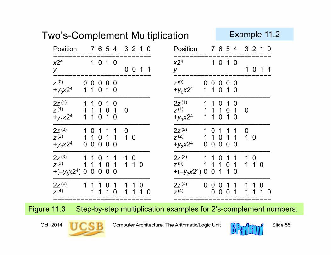
Two’s-Complement Multiplication
Figure 11.3 Step-by-step multiplication examples for 2’s-complement numbers.
Position 7 6 5 4 3 2 1 0 Position 7 6 5 4 3 2 1 0========================= =========================x24 1 0 1 0 x24 1 0 1 0y 0 0 1 1 y 1 0 1 1========================= =========================z (0) 0 0 0 0 0 z (0) 0 0 0 0 0+y0x24 1 1 0 1 0 +y0x24 1 1 0 1 0–––––––––––––––––––––––––– ––––––––––––––––––––––––––2z (1) 1 1 0 1 0 2z (1) 1 1 0 1 0z (1) 1 1 1 0 1 0 z (1) 1 1 1 0 1 0+y1x24 1 1 0 1 0 +y1x24 1 1 0 1 0–––––––––––––––––––––––––– ––––––––––––––––––––––––––2z (2) 1 0 1 1 1 0 2z (2) 1 0 1 1 1 0z (2) 1 1 0 1 1 1 0 z (2) 1 1 0 1 1 1 0+y2x24 0 0 0 0 0 +y2x24 0 0 0 0 0–––––––––––––––––––––––––– ––––––––––––––––––––––––––2z (3) 1 1 0 1 1 1 0 2z (3) 1 1 0 1 1 1 0z (3) 1 1 1 0 1 1 1 0 z (3) 1 1 1 0 1 1 1 0+(–y3x24) 0 0 0 0 0 +(–y3x24) 0 0 1 1 0–––––––––––––––––––––––––– ––––––––––––––––––––––––––2z (4) 1 1 1 0 1 1 1 0 2z (4) 0 0 0 1 1 1 1 0z (4) 1 1 1 0 1 1 1 0 z (4) 0 0 0 1 1 1 1 0========================= =========================
Example 11.2
Oct. 2014 Computer Architecture, The Arithmetic/Logic Unit Slide 56
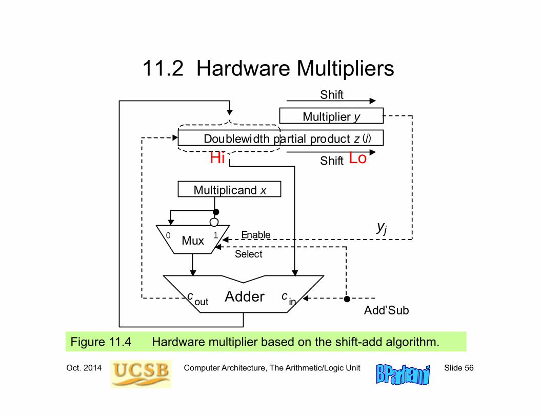
11.2 Hardware Multipliers
Multiplier y
Mux
Adder out c
0 1
Doublewidth partial product z
Multiplicand x
Shift
Shift
(j)
j y
Add’Sub
Enable
Select
in c
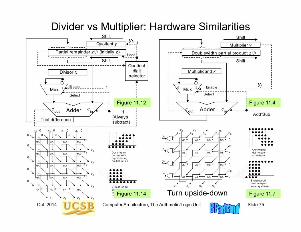
Figure 11.4 Hardware multiplier based on the shift-add algorithm.
Hi Lo
Oct. 2014 Computer Architecture, The Arithmetic/Logic Unit Slide 57
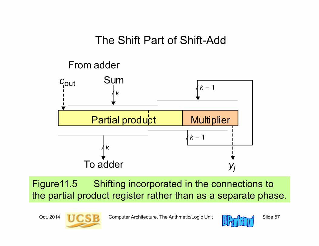
The Shift Part of Shift-Add
Figure11.5 Shifting incorporated in the connections to the partial product register rather than as a separate phase.
out c
To adder j y
From adderSum
Partial product Multiplier
/ k – 1
/ k – 1
/ k
/ k
Oct. 2014 Computer Architecture, The Arithmetic/Logic Unit Slide 58
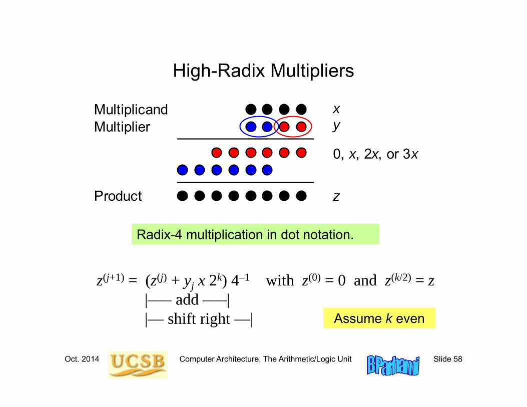
High-Radix Multipliers
Radix-4 multiplication in dot notation.
Multiplicand x y
z
Multiplier
Product
0, x, 2x, or 3x
z(j+1) = (z(j) + yj x 2k) 4–1 with z(0) = 0 and z(k/2) = z|––– add –––||–– shift right ––| Assume k even
Oct. 2014 Computer Architecture, The Arithmetic/Logic Unit Slide 59
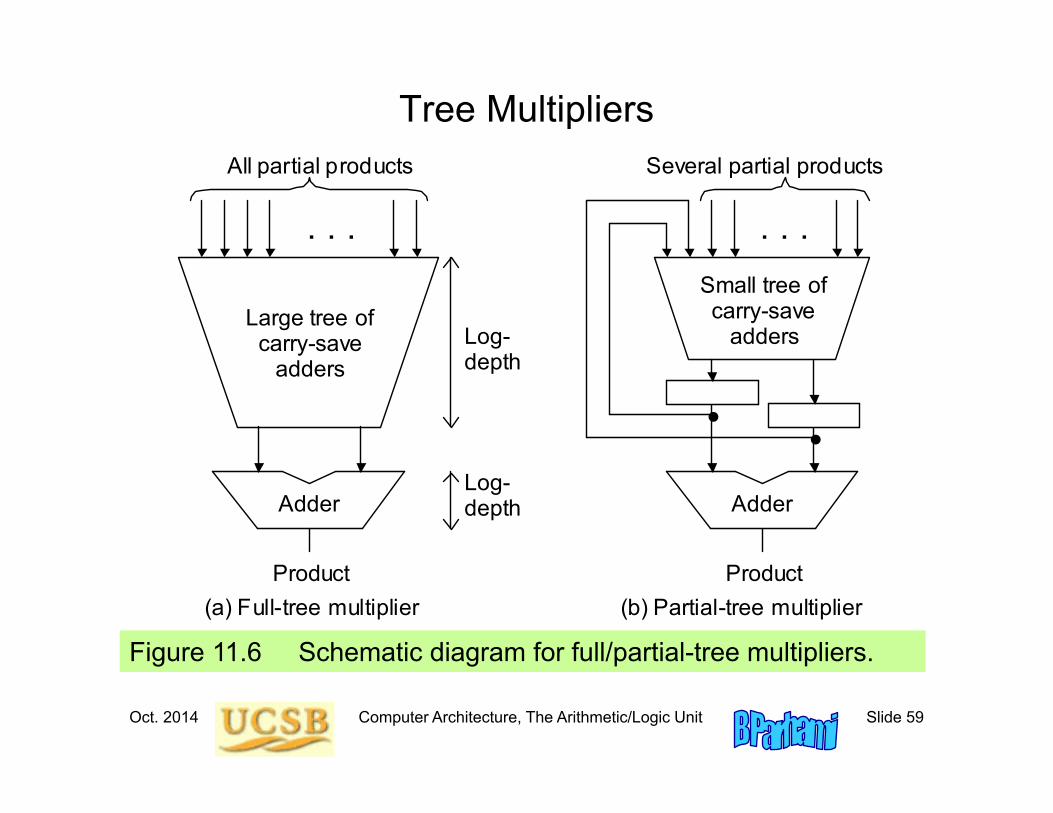
Tree Multipliers
Figure 11.6 Schematic diagram for full/partial-tree multipliers.
Adder
Large tree of carry-save
adders
. . .
All partial products
Product
Adder
Small tree of carry-save
adders
. . .
Several partial products
Product
Log-depth
Log-depth
(a) Full-tree multiplier (b) Partial-tree multiplier
Oct. 2014 Computer Architecture, The Arithmetic/Logic Unit Slide 60
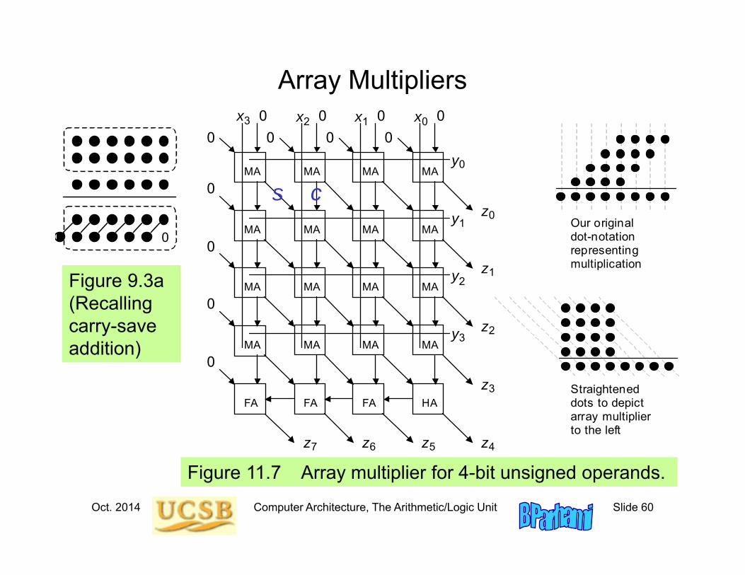
Array Multipliers
Figure 11.7 Array multiplier for 4-bit unsigned operands.
3
2
1
0
4 5 6 7
0
1
2
3
2 1 0 x x x
y
y
y
z
y
3 x
0 0
0 0
0 0
0 0
0
0
0 z
z
z
z z z z
HA FA FA
MA MA MA MA
MA MA MA MA
MA MA MA MA
MA MA MA MA
FA
0
Our original dot-notation representing multiplication
Straightened dots to depict array multiplier to the left
s cs
0
Figure 9.3a (Recalling carry-save addition)
Oct. 2014 Computer Architecture, The Arithmetic/Logic Unit Slide 61
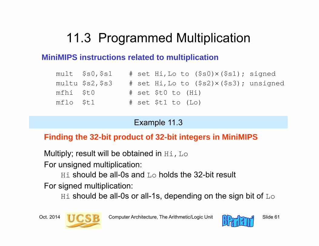
11.3 Programmed MultiplicationMiniMIPS instructions related to multiplication
mult $s0,$s1 # set Hi,Lo to ($s0)($s1); signedmultu $s2,$s3 # set Hi,Lo to ($s2)($s3); unsignedmfhi $t0 # set $t0 to (Hi)mflo $t1 # set $t1 to (Lo)
Finding the 32-bit product of 32-bit integers in MiniMIPS
Multiply; result will be obtained in Hi,LoFor unsigned multiplication:
Hi should be all-0s and Lo holds the 32-bit resultFor signed multiplication:
Hi should be all-0s or all-1s, depending on the sign bit of Lo
Example 11.3
Oct. 2014 Computer Architecture, The Arithmetic/Logic Unit Slide 62
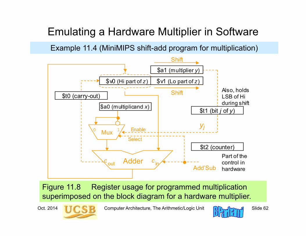
Figure 11.8 Register usage for programmed multiplication superimposed on the block diagram for a hardware multiplier.
Emulating a Hardware Multiplier in Software
$t2 (counter) Part of thecontrol in hardware
Also, holdsLSB of Hi during shift
Multiplier y
Mux
Adder out
c
0 1
Doublewidth partial product z
Multiplicand x
Shift
Shift
(j)
j
y
Add’Sub
Enable
Select
in
c
$a0 (multiplicand x)
$a1 (multiplier y)
$v1 (Lo part of z) $v0 (Hi part of z)
$t0 (carry-out)
$t1 (bit j of y)
Example 11.4 (MiniMIPS shift-add program for multiplication)

Oct. 2014 Computer Architecture, The Arithmetic/Logic Unit Slide 63
shamu: move $v0,$zero # initialize Hi to 0move $vl,$zero # initialize Lo to 0addi $t2,$zero,32 # init repetition counter to 32
mloop: move $t0,$zero # set c-out to 0 in case of no addmove $t1,$a1 # copy ($a1) into $t1srl $a1,1 # halve the unsigned value in $a1subu $t1,$t1,$a1 # subtract ($a1) from ($t1) twice tosubu $t1,$t1,$a1 # obtain LSB of ($a1), or y[j], in $t1beqz $t1,noadd # no addition needed if y[j] = 0addu $v0,$v0,$a0 # add x to upper part of zsltu $t0,$v0,$a0 # form carry-out of addition in $t0
noadd: move $t1,$v0 # copy ($v0) into $t1srl $v0,1 # halve the unsigned value in $v0subu $t1,$t1,$v0 # subtract ($v0) from ($t1) twice tosubu $t1,$t1,$v0 # obtain LSB of Hi in $t1sll $t0,$t0,31 # carry-out converted to 1 in MSB of $t0addu $v0,$v0,$t0 # right-shifted $v0 correctedsrl $v1,1 # halve the unsigned value in $v1sll $t1,$t1,31 # LSB of Hi converted to 1 in MSB of $t1addu $v1,$v1,$t1 # right-shifted $v1 correctedaddi $t2,$t2,-1 # decrement repetition counter by 1bne $t2,$zero,mloop # if counter > 0, repeat multiply loopjr $ra # return to the calling program
Multiplication When There Is No Multiply InstructionExample 11.4 (MiniMIPS shift-add program for multiplication)
Oct. 2014 Computer Architecture, The Arithmetic/Logic Unit Slide 64
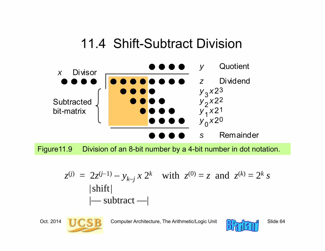
11.4 Shift-Subtract Division
Figure11.9 Division of an 8-bit number by a 4-bit number in dot notation.
z(j) = 2z(j1) ykj x 2k with z(0) = z and z(k) = 2k s| shift ||–– subtract ––|
2 1
2
y
2
x 2
2
1 0
3
0
Subtracted bit-matrix
Divisor x Dividend z
s Remainder
Quotient y
y x 3 y x 2 y x
Oct. 2014 Computer Architecture, The Arithmetic/Logic Unit Slide 65
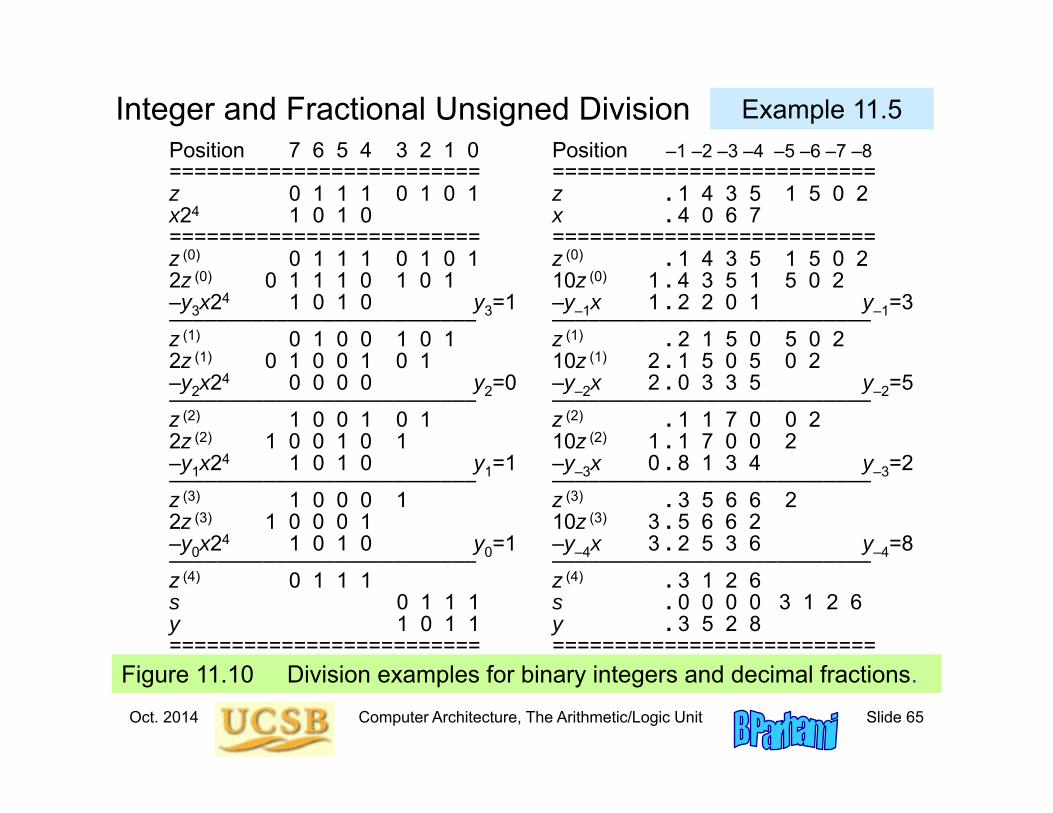
Integer and Fractional Unsigned Division
Figure 11.10 Division examples for binary integers and decimal fractions.
Position 7 6 5 4 3 2 1 0 Position –1 –2 –3 –4 –5 –6 –7 –8========================= ==========================z 0 1 1 1 0 1 0 1 z . 1 4 3 5 1 5 0 2x24 1 0 1 0 x . 4 0 6 7========================= ==========================z (0) 0 1 1 1 0 1 0 1 z (0) . 1 4 3 5 1 5 0 22z (0) 0 1 1 1 0 1 0 1 10z (0) 1 . 4 3 5 1 5 0 2–y3x24 1 0 1 0 y3=1 –y–1x 1 . 2 2 0 1 y–1=3–––––––––––––––––––––––––– –––––––––––––––––––––––––––z (1) 0 1 0 0 1 0 1 z (1) . 2 1 5 0 5 0 22z (1) 0 1 0 0 1 0 1 10z (1) 2 . 1 5 0 5 0 2–y2x24 0 0 0 0 y2=0 –y–2x 2 . 0 3 3 5 y–2=5–––––––––––––––––––––––––– –––––––––––––––––––––––––––z (2) 1 0 0 1 0 1 z (2) . 1 1 7 0 0 22z (2) 1 0 0 1 0 1 10z (2) 1 . 1 7 0 0 2–y1x24 1 0 1 0 y1=1 –y–3x 0 . 8 1 3 4 y–3=2–––––––––––––––––––––––––– –––––––––––––––––––––––––––z (3) 1 0 0 0 1 z (3) . 3 5 6 6 22z (3) 1 0 0 0 1 10z (3) 3 . 5 6 6 2–y0x24 1 0 1 0 y0=1 –y–4x 3 . 2 5 3 6 y–4=8–––––––––––––––––––––––––– –––––––––––––––––––––––––––z (4) 0 1 1 1 z (4) . 3 1 2 6s 0 1 1 1 s . 0 0 0 0 3 1 2 6y 1 0 1 1 y . 3 5 2 8========================= ==========================
Example 11.5
Oct. 2014 Computer Architecture, The Arithmetic/Logic Unit Slide 66
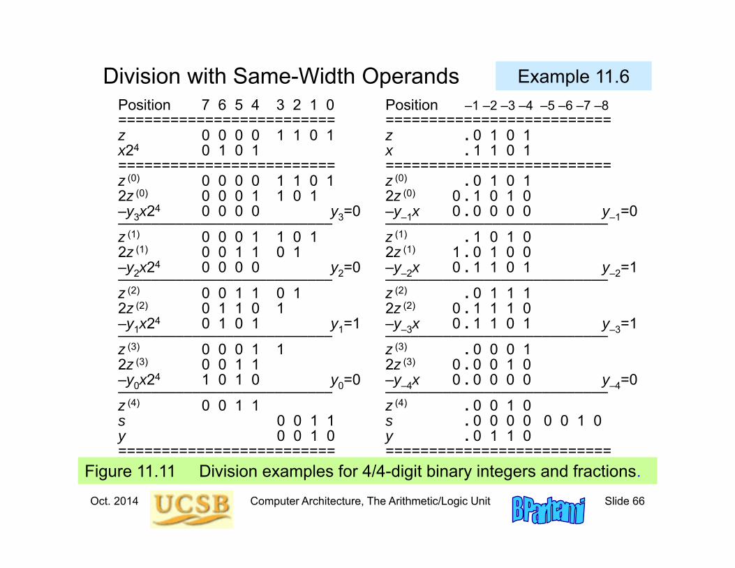
Division with Same-Width Operands
Figure 11.11 Division examples for 4/4-digit binary integers and fractions.
Position 7 6 5 4 3 2 1 0 Position –1 –2 –3 –4 –5 –6 –7 –8========================= ==========================z 0 0 0 0 1 1 0 1 z . 0 1 0 1x24 0 1 0 1 x . 1 1 0 1========================= ==========================z (0) 0 0 0 0 1 1 0 1 z (0) . 0 1 0 12z (0) 0 0 0 1 1 0 1 2z (0) 0 . 1 0 1 0–y3x24 0 0 0 0 y3=0 –y–1x 0 . 0 0 0 0 y–1=0–––––––––––––––––––––––––– –––––––––––––––––––––––––––z (1) 0 0 0 1 1 0 1 z (1) . 1 0 1 0 2z (1) 0 0 1 1 0 1 2z (1) 1 . 0 1 0 0–y2x24 0 0 0 0 y2=0 –y–2x 0 . 1 1 0 1 y–2=1–––––––––––––––––––––––––– –––––––––––––––––––––––––––z (2) 0 0 1 1 0 1 z (2) . 0 1 1 12z (2) 0 1 1 0 1 2z (2) 0 . 1 1 1 0 –y1x24 0 1 0 1 y1=1 –y–3x 0 . 1 1 0 1 y–3=1–––––––––––––––––––––––––– –––––––––––––––––––––––––––z (3) 0 0 0 1 1 z (3) . 0 0 0 12z (3) 0 0 1 1 2z (3) 0 . 0 0 1 0–y0x24 1 0 1 0 y0=0 –y–4x 0 . 0 0 0 0 y–4=0–––––––––––––––––––––––––– –––––––––––––––––––––––––––z (4) 0 0 1 1 z (4) . 0 0 1 0s 0 0 1 1 s . 0 0 0 0 0 0 1 0y 0 0 1 0 y . 0 1 1 0========================= ==========================
Example 11.6
Oct. 2014 Computer Architecture, The Arithmetic/Logic Unit Slide 67
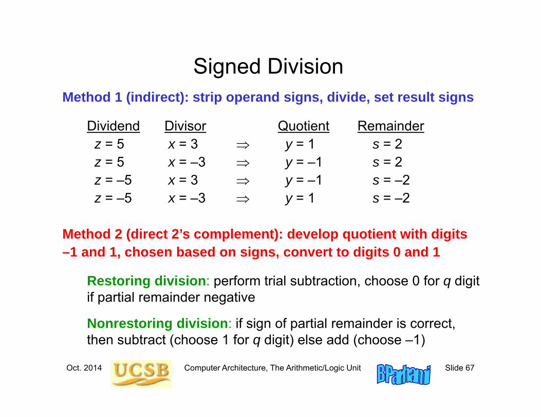
Signed DivisionMethod 1 (indirect): strip operand signs, divide, set result signs
Dividend Divisor Quotient Remainderz = 5 x = 3 y = 1 s = 2z = 5 x = –3 y = –1 s = 2z = –5 x = 3 y = –1 s = –2z = –5 x = –3 y = 1 s = –2
Method 2 (direct 2’s complement): develop quotient with digits–1 and 1, chosen based on signs, convert to digits 0 and 1
Restoring division: perform trial subtraction, choose 0 for q digitif partial remainder negative
Nonrestoring division: if sign of partial remainder is correct,then subtract (choose 1 for q digit) else add (choose –1)
Oct. 2014 Computer Architecture, The Arithmetic/Logic Unit Slide 68
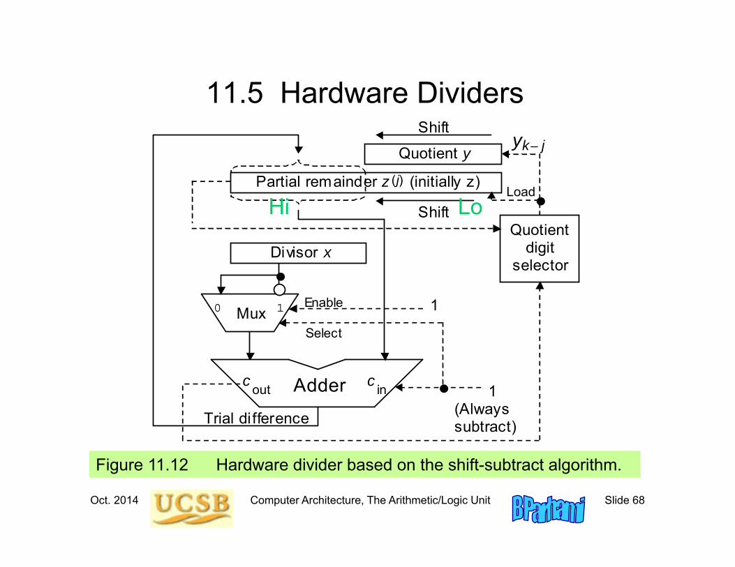
11.5 Hardware Dividers
Figure 11.12 Hardware divider based on the shift-subtract algorithm.
Load
Quotient y
Mux
Adder
0 1
Partial remainder z (initially z)
Divisor x
Shift
Shift
(j)
k– j
y
1
Enable
Select
Quotient
digit selector
1
out
c in
c
Trial di fference (Always subtract)
Hi Lo
Oct. 2014 Computer Architecture, The Arithmetic/Logic Unit Slide 69
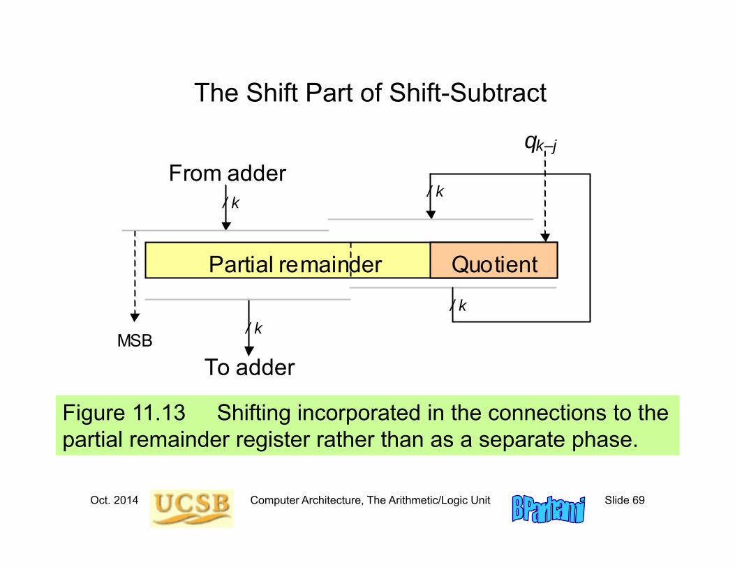
The Shift Part of Shift-Subtract
Figure 11.13 Shifting incorporated in the connections to the partial remainder register rather than as a separate phase.
To adder
From adder
Partial remainder Quotient
/ k
/ k
/ k
/ k
k–j q
MSB
Oct. 2014 Computer Architecture, The Arithmetic/Logic Unit Slide 70
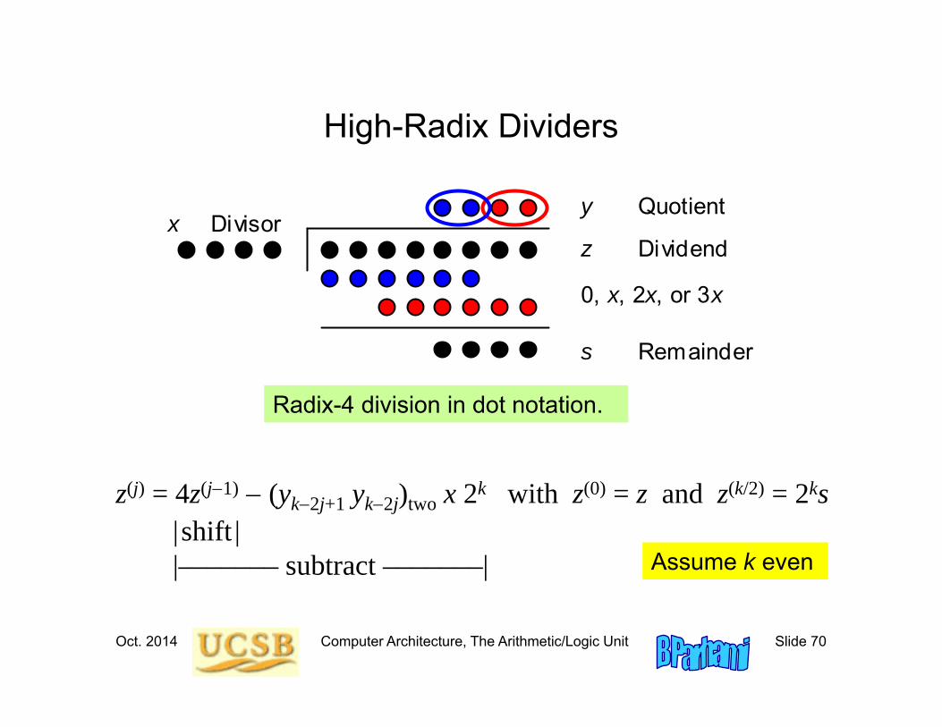
High-Radix Dividers
Radix-4 division in dot notation.
Divisor x Dividend z
s Remainder
Quotient y
0, x, 2x, or 3x
z(j) = 4z(j1) (yk2j+1 yk2j)two x 2k with z(0) = z and z(k/2) = 2ks| shift ||––––––– subtract –––––––| Assume k even
Oct. 2014 Computer Architecture, The Arithmetic/Logic Unit Slide 71
Array Dividers
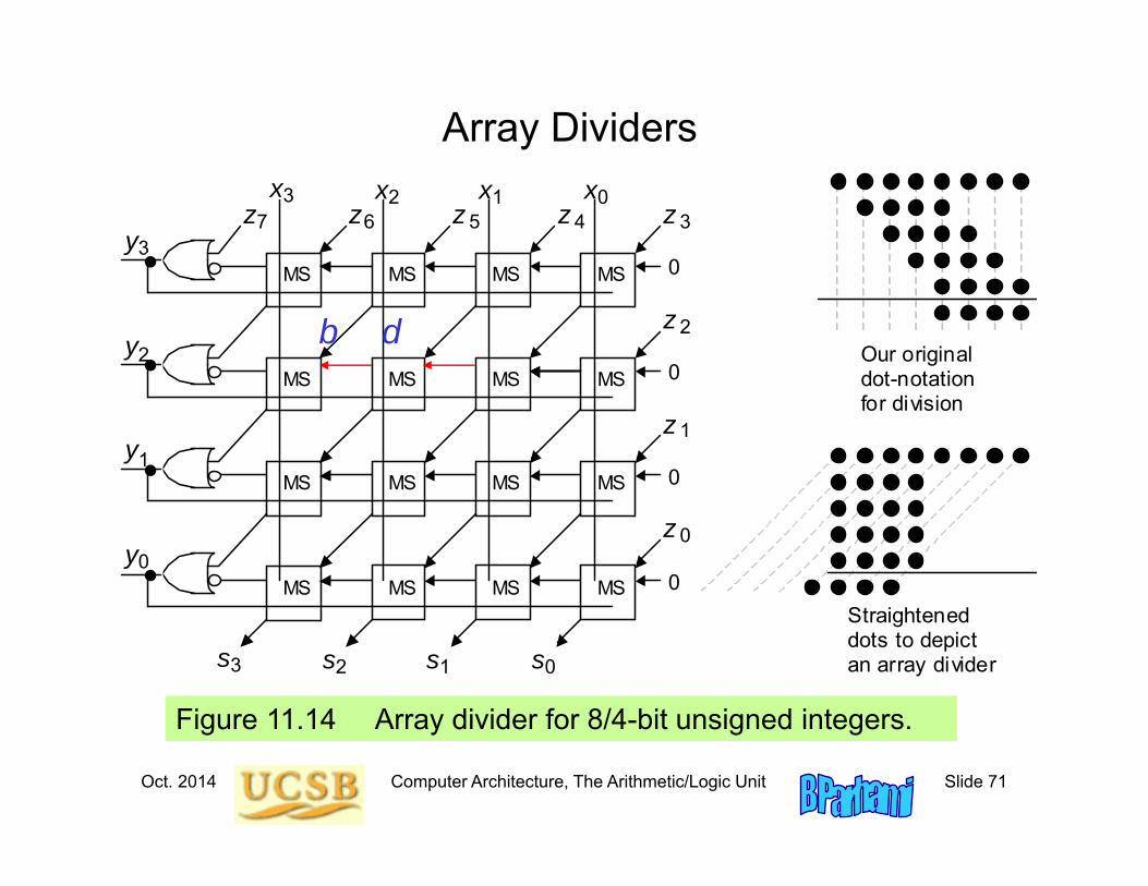
Figure 11.14 Array divider for 8/4-bit unsigned integers.
2 1 0 x x x
1 y
2 y
3 y 3 z
0 y
3 x
2 z
1 z
0 z
4 z 5 z 6 z 7 z
MS MS MS MS
MS MS MS MS
MS MS MS MS
MS MS MS MS
Our original dot-notation for division
Straightened dots to depict an array divider 2 1 0 s s s 3 s
0
0
0
0
b d
Oct. 2014 Computer Architecture, The Arithmetic/Logic Unit Slide 72
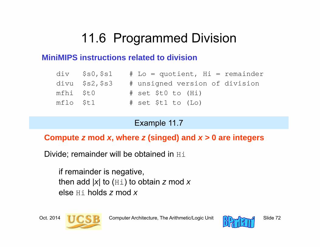
11.6 Programmed DivisionMiniMIPS instructions related to division
div $s0,$s1 # Lo = quotient, Hi = remainderdivu $s2,$s3 # unsigned version of divisionmfhi $t0 # set $t0 to (Hi)mflo $t1 # set $t1 to (Lo)
Compute z mod x, where z (singed) and x > 0 are integers
Divide; remainder will be obtained in Hi
if remainder is negative,then add |x| to (Hi) to obtain z mod xelse Hi holds z mod x
Example 11.7
Oct. 2014 Computer Architecture, The Arithmetic/Logic Unit Slide 73
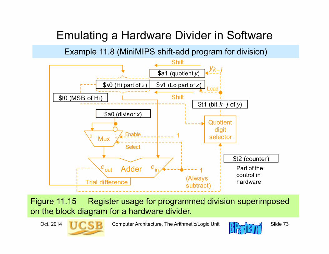
Figure 11.15 Register usage for programmed division superimposed on the block diagram for a hardware divider.
Emulating a Hardware Divider in SoftwareExample 11.8 (MiniMIPS shift-add program for division)
Load
Quotient y
Mux
Adder
0 1
Partial remainder z (initially z)
Divisor x
Shift
Shift
(j)
k– j
y
1
Enable Select
Quotient digit
selector
1
out
c
in
c Trial difference
(Always subtract)
$t2 (counter)
$a0 (divisor x)
$a1 (quotient y)
$v1 (Lo part of z) $v0 (Hi part of z)
$t1 (bit kj of y)
Part of the control in hardware
$t0 (MSB of Hi)
Oct. 2014 Computer Architecture, The Arithmetic/Logic Unit Slide 74
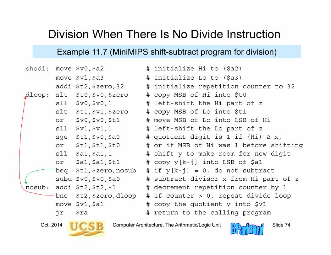
shsdi: move $v0,$a2 # initialize Hi to ($a2)
move $vl,$a3 # initialize Lo to ($a3)addi $t2,$zero,32 # initialize repetition counter to 32
dloop: slt $t0,$v0,$zero # copy MSB of Hi into $t0sll $v0,$v0,1 # left-shift the Hi part of zslt $t1,$v1,$zero # copy MSB of Lo into $t1or $v0,$v0,$t1 # move MSB of Lo into LSB of Hisll $v1,$v1,1 # left-shift the Lo part of zsge $t1,$v0,$a0 # quotient digit is 1 if (Hi) x,or $t1,$t1,$t0 # or if MSB of Hi was 1 before shiftingsll $a1,$a1,1 # shift y to make room for new digitor $a1,$a1,$t1 # copy y[k-j] into LSB of $a1beq $t1,$zero,nosub # if y[k-j] = 0, do not subtractsubu $v0,$v0,$a0 # subtract divisor x from Hi part of z
nosub: addi $t2,$t2,-1 # decrement repetition counter by 1bne $t2,$zero,dloop # if counter > 0, repeat divide loopmove $v1,$a1 # copy the quotient y into $v1jr $ra # return to the calling program
Division When There Is No Divide InstructionExample 11.7 (MiniMIPS shift-subtract program for division)
Oct. 2014 Computer Architecture, The Arithmetic/Logic Unit Slide 75
Load
Quotient y
Mux
Adder
0 1
Partial remainder z (initially z)
Divisor x
Shift
Shift
(j)
k– j
y
1
Enable
Select
Quotient
digit selector
1
out
c in
c
Trial di fference (Always subtract)
Multiplier y
Mux
Adder out c
0 1
Doublewidth partial product z
Multiplicand x
Shift
Shift
(j)
j y
Add’Sub
Enable
Select
in c
Divider vs Multiplier: Hardware Similarities
2 1 0 x x x
1 y
2 y
3 y 3 z
0 y
3 x
2 z
1 z
0 z
4 z 5 z 6 z 7 z
MS MS MS MS
MS MS MS MS
MS MS MS MS
MS MS MS MS
Our original dot-notation for division
Straightened dots to depict an array divider 2 1 0 s s s 3 s
0
0
0
0
Figure 11.12 Figure 11.4
3
2
1
0
4 5 6 7
0
1
2
3
2 1 0 x x x
y
y
y
z
y
3 x
0 0
0 0
0 0
0 0
0
0
0 z
z
z
z z z z
HA FA FA
MA MA MA MA
MA MA MA MA
MA MA MA MA
MA MA MA MA
FA
0
Our o rigin al dot-n otation rep resentin g m ultiplication
S traighten ed dots to depic t array m ultiplier to the left Figure 11.14 Figure 11.7Turn upside-down
Oct. 2014 Computer Architecture, The Arithmetic/Logic Unit Slide 76
12 Floating-Point ArithmeticFloating-point is no longer reserved for high-end machines
• Multimedia and signal processing require flp arithmetic• Details of standard flp format and arithmetic operations
Topics in This Chapter
12.1 Rounding Modes
12.2 Special Values and Exceptions
12.3 Floating-Point Addition
12.4 Other Floating-Point Operations
12.5 Floating-Point Instructions
12.6 Result Precision and Errors
Oct. 2014 Computer Architecture, The Arithmetic/Logic Unit Slide 77
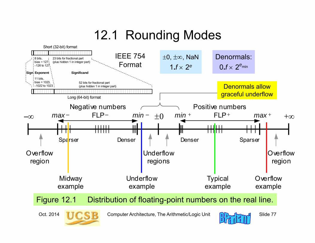
12.1 Rounding Modes
Figure 12.1 Distribution of floating-point numbers on the real line.
Denser Denser Sparser Sparser
Negative numbers FLP FLP 0 +
–
Overflow region
Overflow region
Underflow regions
Positive numbers
Underflow example
Overflow example
Midway example
Typical example
min max min max + + – – – +
Denormals allow graceful underflow
Short (32-bit) format
Long (64-bit) format
Sign Exponent Significand
8 bits, bias = 127, –126 to 127
11 bits, bias = 1023, –1022 to 1023
52 bits for fractional part (plus hidden 1 in integer part)
23 bits for fractional part (plus hidden 1 in integer part)
IEEE 754Format
0, , NaN1.f 2e
Denormals:0.f 2emin

Oct. 2014 Computer Architecture, The Arithmetic/Logic Unit Slide 78
Figure 12.2 Two round-to-nearest-integer functions for x in [–4, 4].
Round-to-Nearest (Even)rtnei(x)
–4
–3
–2
–1
x–4 –3 –2 –1 4 3 2 1
4
3
2
1
rtni(x)
–4
–3
–2
–1
x–4 –3 –2 –1 4 3 2 1
4
3
2
1
(a) Round to nearest even integer (b) Round to nearest integer
Oct. 2014 Computer Architecture, The Arithmetic/Logic Unit Slide 79
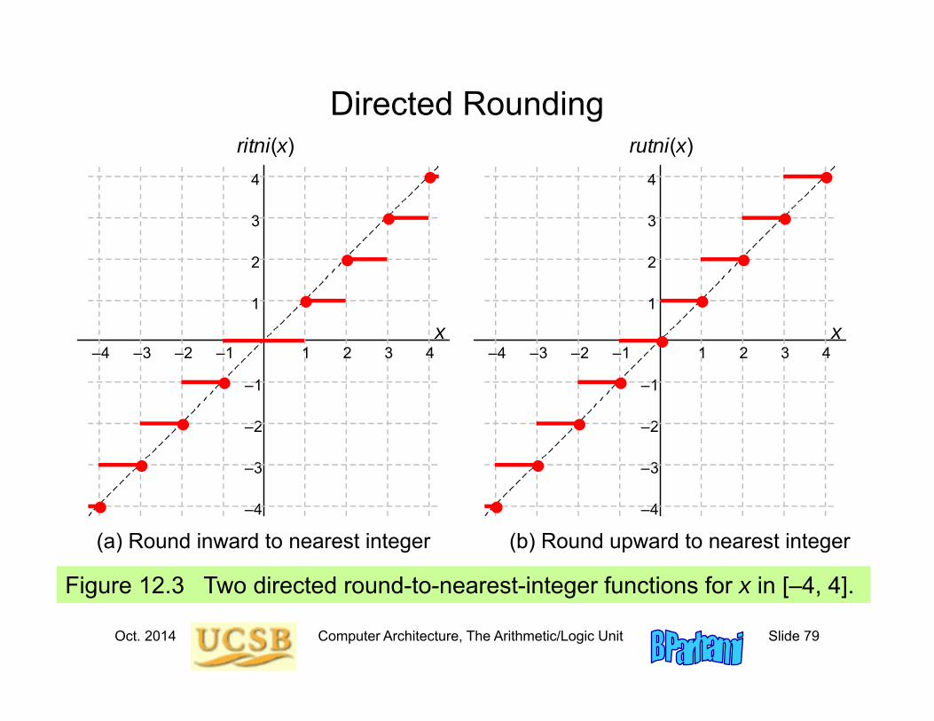
Figure 12.3 Two directed round-to-nearest-integer functions for x in [–4, 4].
Directed Rounding
(a) Round inward to nearest integer (b) Round upward to nearest integer
rutni(x)
–4
–3
–2
–1
x–4 –3 –2 –1 4 3 2 1
4
3
2
1
ritni(x)
–4
–3
–2
–1
x–4 –3 –2 –1 4 3 2 1
4
3
2
1
Oct. 2014 Computer Architecture, The Arithmetic/Logic Unit Slide 80
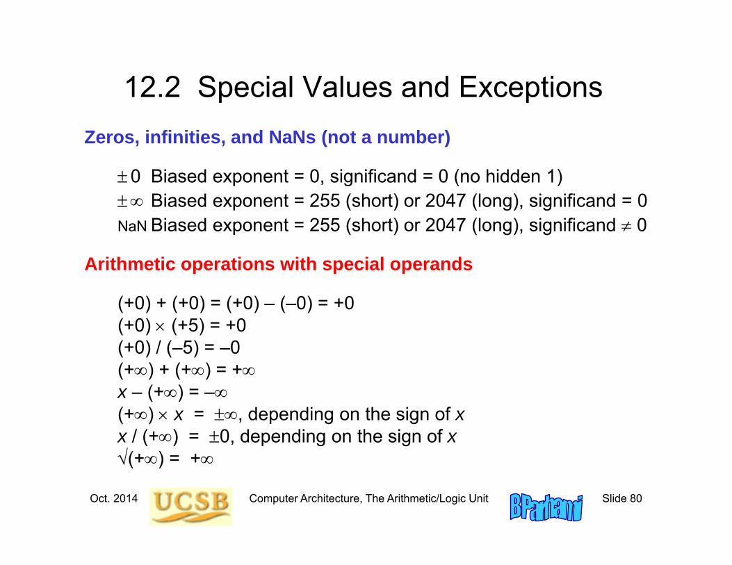
12.2 Special Values and ExceptionsZeros, infinities, and NaNs (not a number)
0 Biased exponent = 0, significand = 0 (no hidden 1) Biased exponent = 255 (short) or 2047 (long), significand = 0NaN Biased exponent = 255 (short) or 2047 (long), significand 0
Arithmetic operations with special operands
(+0) + (+0) = (+0) – (–0) = +0(+0) (+5) = +0(+0) / (–5) = –0(+) + (+) = +x – (+) = –(+) x = , depending on the sign of xx / (+) = 0, depending on the sign of x(+) = +
Oct. 2014 Computer Architecture, The Arithmetic/Logic Unit Slide 81
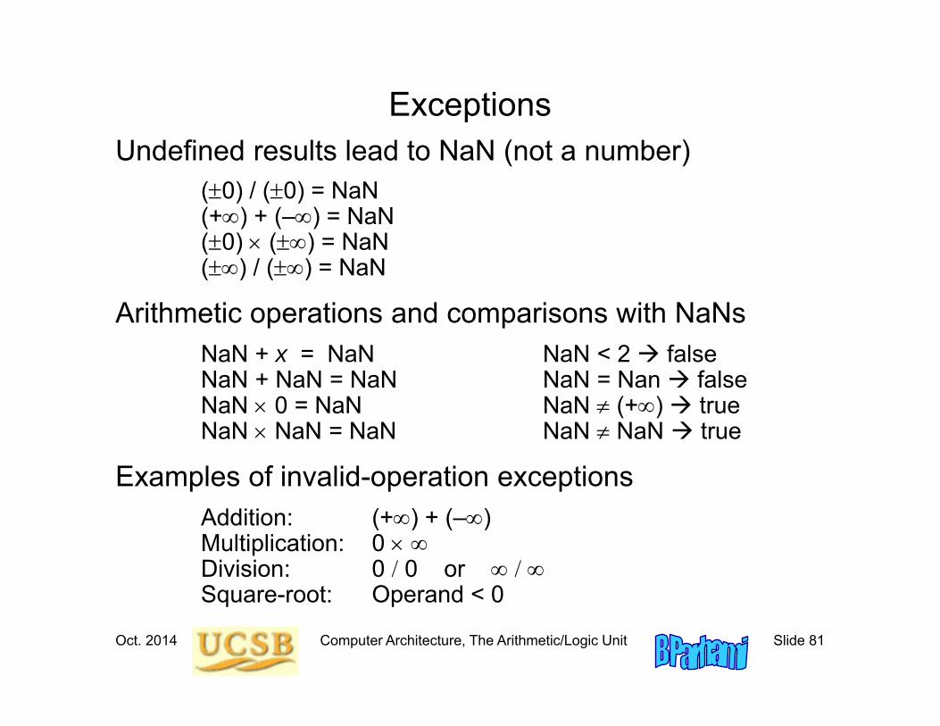
ExceptionsUndefined results lead to NaN (not a number)
(0) / (0) = NaN(+) + (–) = NaN(0) () = NaN() / () = NaN
Arithmetic operations and comparisons with NaNsNaN + x = NaN NaN < 2 falseNaN + NaN = NaN NaN = Nan falseNaN 0 = NaN NaN (+) trueNaN NaN = NaN NaN NaN true
Examples of invalid-operation exceptionsAddition: (+) + (–)Multiplication: 0 Division: 0 0 or Square-root: Operand < 0
Oct. 2014 Computer Architecture, The Arithmetic/Logic Unit Slide 82
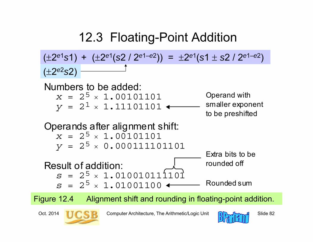
12.3 Floating-Point Addition
Figure 12.4 Alignment shift and rounding in floating-point addition.
Operands after alignment shift: x = 2 1.00101101 y = 2 0.000111101101
Numbers to be added: x = 2 1.00101101 y = 2 1.11101101
5
5
Extra bits to be rounded off
Operand with smaller exponent to be preshifted
Result of addition: s = 2 1.010010111101 s = 2 1.01001100 Rounded sum
5
1
5 5
(2e1s1) (2e2s2)
+ (2e1(s2 / 2e1–e2)) = 2e1(s1 s2 / 2e1–e2)
Oct. 2014 Computer Architecture, The Arithmetic/Logic Unit Slide 83
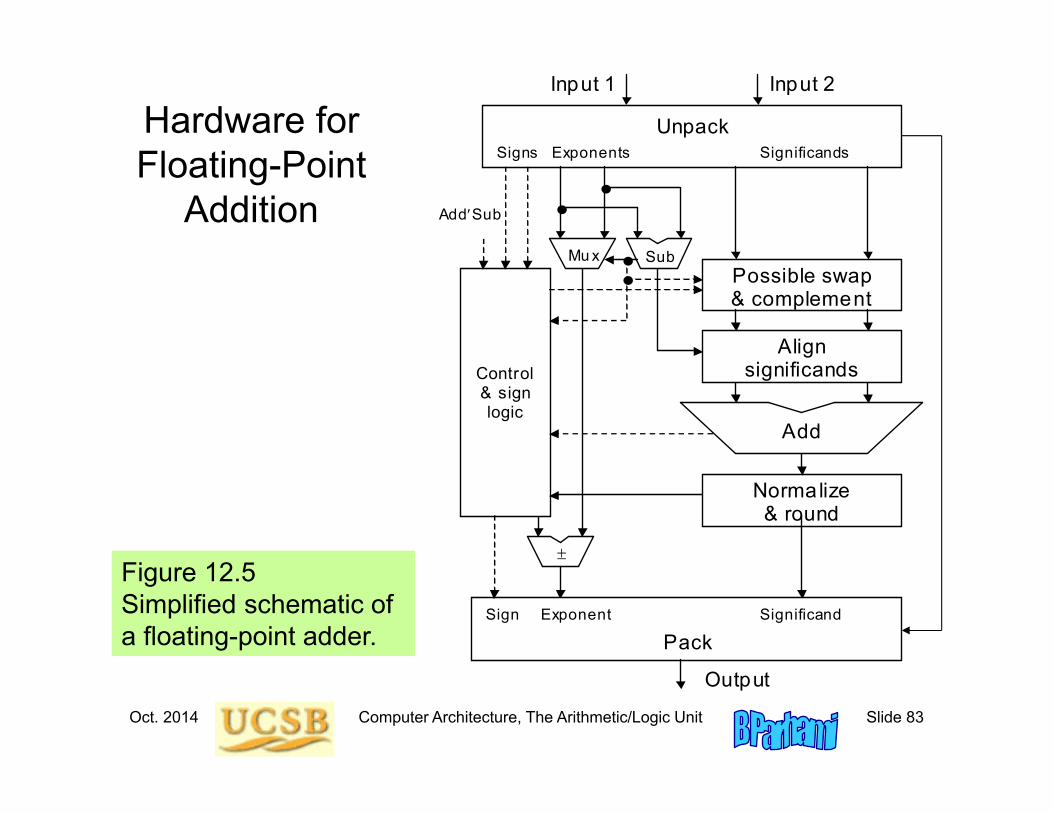
Hardware for Floating-Point
Addition
Figure 12.5 Simplified schematic of a floating-point adder.
Normalize & round
Add
Align significands
Possible swap & complement
Unpack
Control & sign logic
Pack
Input 1
Output
Significands Exponents Signs
Significand Exponent Sign
Sub
Mu x
Input 2
AddSub
Oct. 2014 Computer Architecture, The Arithmetic/Logic Unit Slide 84
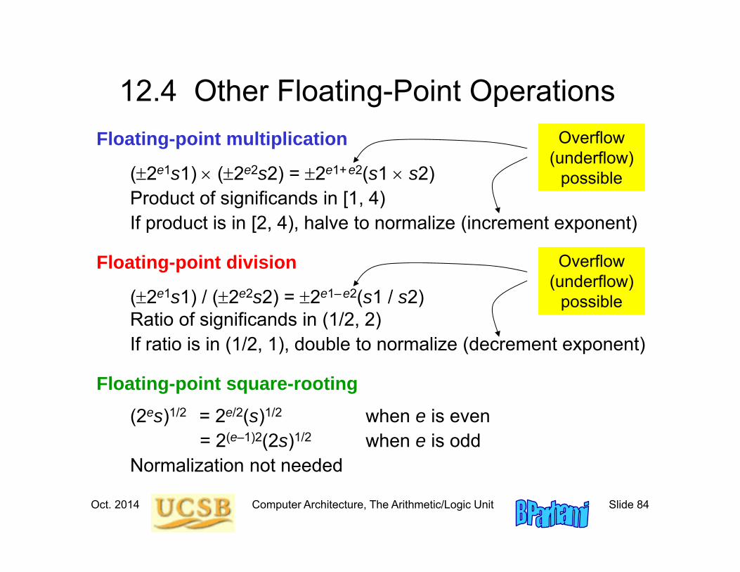
12.4 Other Floating-Point OperationsFloating-point multiplication
(2e1s1) (2e2s2) = 2e1+ e2(s1 s2)Product of significands in [1, 4)If product is in [2, 4), halve to normalize (increment exponent)
Floating-point division
(2e1s1) / (2e2s2) = 2e1– e2(s1 / s2)Ratio of significands in (1/2, 2)If ratio is in (1/2, 1), double to normalize (decrement exponent)
Floating-point square-rooting(2es)1/2 = 2e/2(s)1/2 when e is even
= 2(e–1)2(2s)1/2 when e is oddNormalization not needed
Overflow (underflow)
possible
Overflow (underflow)
possible
Oct. 2014 Computer Architecture, The Arithmetic/Logic Unit Slide 85
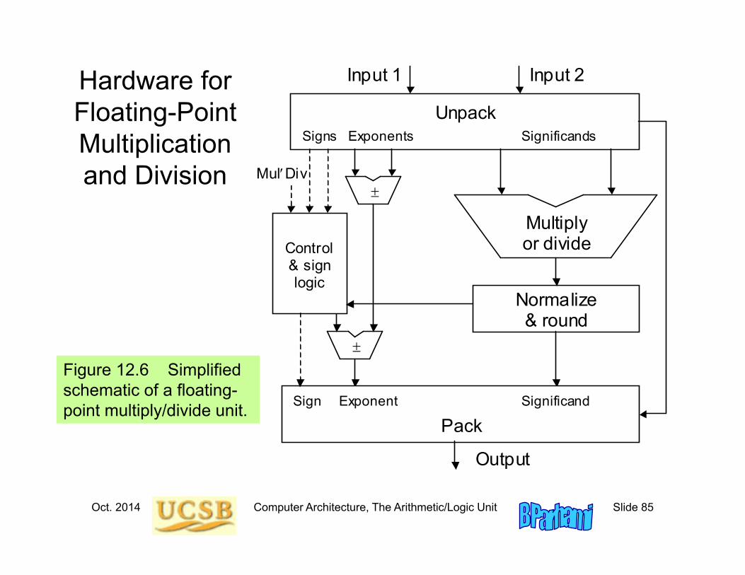
Hardware for Floating-Point Multiplication and Division
Figure 12.6 Simplified schematic of a floating-point multiply/divide unit.
Normalize & round
Multiply or divide
Unpack
Control & sign logic
MulDiv
Pack
Input 1
Output
Significands Exponents Signs
Significand Exponent Sign
Input 2
Oct. 2014 Computer Architecture, The Arithmetic/Logic Unit Slide 86
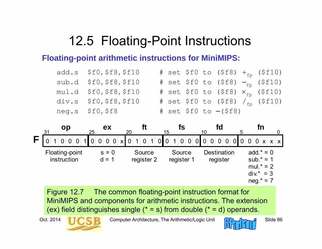
12.5 Floating-Point InstructionsFloating-point arithmetic instructions for MiniMIPS:
add.s $f0,$f8,$f10 # set $f0 to ($f8) +fp ($f10)sub.d $f0,$f8,$f10 # set $f0 to ($f8) –fp ($f10)mul.d $f0,$f8,$f10 # set $f0 to ($f8) fp ($f10)div.s $f0,$f8,$f10 # set $f0 to ($f8) /fp ($f10)neg.s $f0,$f8 # set $f0 to –($f8)
Figure 12.7 The common floating-point instruction format for MiniMIPS and components for arithmetic instructions. The extension (ex) field distinguishes single (* = s) from double (* = d) operands.
x x x x 0 1 1 0 0 0 0 0 0 0 0 0 0 0 0 0 0 1 1 1 0 0 0 0 0 0 0 0 31 25 20 15 0
Floating-point instruction
s = 0 d = 1
Source register 2
op ex ft
F fs fd
10 5 fn
Destination register
add.* = 0 sub.* = 1 mul.* = 2 div.* = 3 neg.* = 7
Source register 1
Oct. 2014 Computer Architecture, The Arithmetic/Logic Unit Slide 87
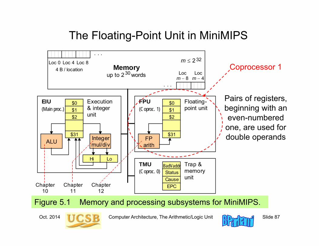
The Floating-Point Unit in MiniMIPS
Figure 5.1 Memory and processing subsystems for MiniMIPS.
Memory up to 2 words 30
Loc 0 Loc 4 Loc 8
Loc m 4
Loc m 8
4 B / location
m 2 32
$0 $1 $2
$31
Hi Lo
ALU
$0 $1 $2
$31 FP
arith
EPC Cause
BadVaddr Status
EIU FPU
TMU
Execution & integer unit
Floating- point unit
Trap & memory unit
. . .
. . .
(Coproc. 1)
(Coproc. 0)
(Main proc.)
Integer mul/div
Chapter 10
Chapter 11
Chapter 12
Pairs of registers, beginning with an even-numbered
one, are used for double operands
Coprocessor 1
Oct. 2014 Computer Architecture, The Arithmetic/Logic Unit Slide 88
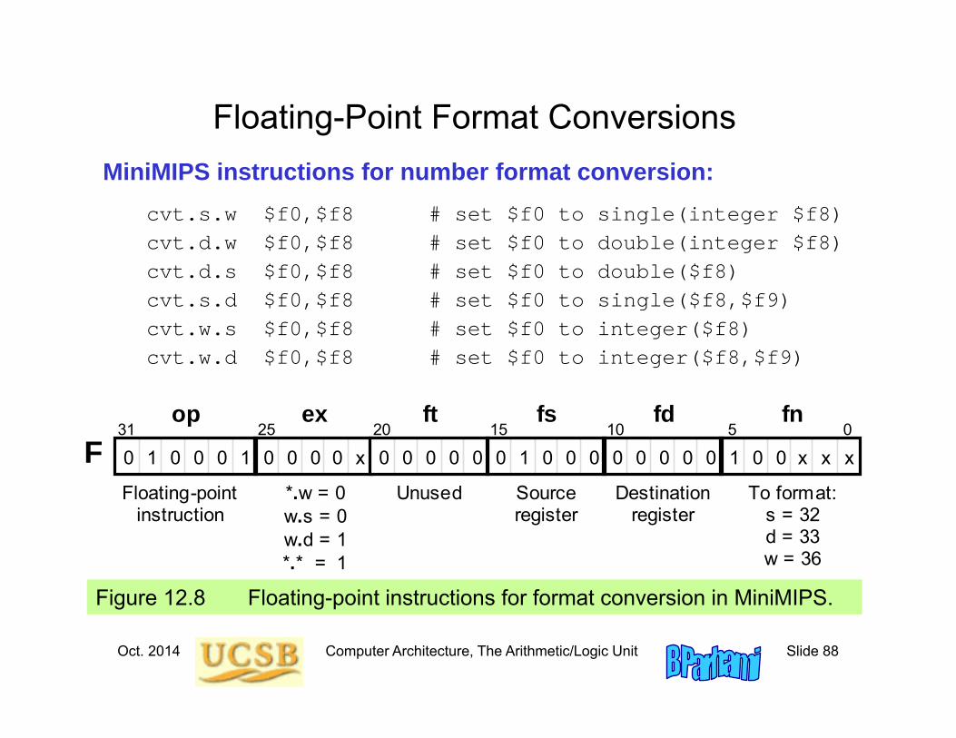
Floating-Point Format ConversionsMiniMIPS instructions for number format conversion:
cvt.s.w $f0,$f8 # set $f0 to single(integer $f8)cvt.d.w $f0,$f8 # set $f0 to double(integer $f8)cvt.d.s $f0,$f8 # set $f0 to double($f8)cvt.s.d $f0,$f8 # set $f0 to single($f8,$f9)cvt.w.s $f0,$f8 # set $f0 to integer($f8)cvt.w.d $f0,$f8 # set $f0 to integer($f8,$f9)
Figure 12.8 Floating-point instructions for format conversion in MiniMIPS.
1 0 0 x x x x 0 1 1 0 0 0 0 0 0 0 0 0 0 0 0 0 0 1 0 0 0 0 0 0 0 31 25 20 15 0
Floating-point instruction
*.w = 0 w.s = 0 w.d = 1 *.* = 1
Unused
op ex ft
F fs fd
10 5 fn
Destination register
To format: s = 32 d = 33 w = 36
Source register
Oct. 2014 Computer Architecture, The Arithmetic/Logic Unit Slide 89
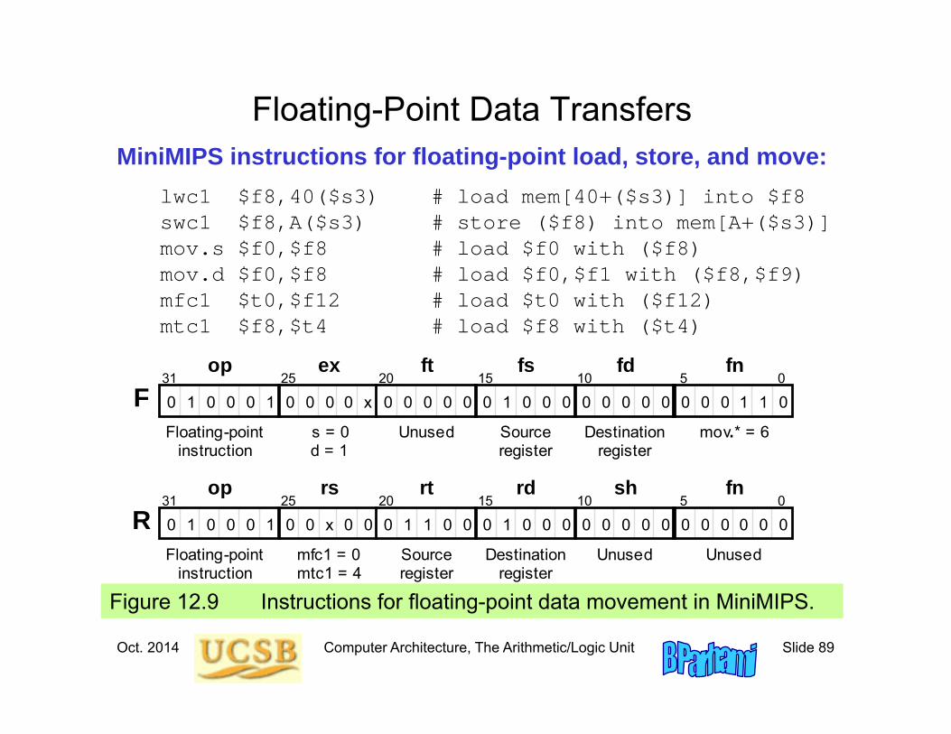
Floating-Point Data TransfersMiniMIPS instructions for floating-point load, store, and move:
lwc1 $f8,40($s3) # load mem[40+($s3)] into $f8swc1 $f8,A($s3) # store ($f8) into mem[A+($s3)]mov.s $f0,$f8 # load $f0 with ($f8)mov.d $f0,$f8 # load $f0,$f1 with ($f8,$f9)mfc1 $t0,$f12 # load $t0 with ($f12)mtc1 $f8,$t4 # load $f8 with ($t4)
Figure 12.9 Instructions for floating-point data movement in MiniMIPS.
0 1 1 0 0 x 0 1 1 0 0 0 0 0 0 0 0 0 0 0 0 0 0 1 0 0 0 0 0 0 0 0 31 25 20 15 0
Floating-point instruction
s = 0 d = 1
Unused
op ex ft
F fs fd
10 5 fn
Destination register
mov.* = 6
Source register
1 1 1 0 0 0 0 x 0 1 1 0 0 0 0 0 0 0 0 0 0 0 0 0 0 0 0 0 0 0 0 0 31 25 20 15 0
Floating-point instruction
mfc1 = 0 mtc1 = 4
Unused
op rs rt
R rd sh
10 5 fn
Destination register
Source register
Unused
Oct. 2014 Computer Architecture, The Arithmetic/Logic Unit Slide 90
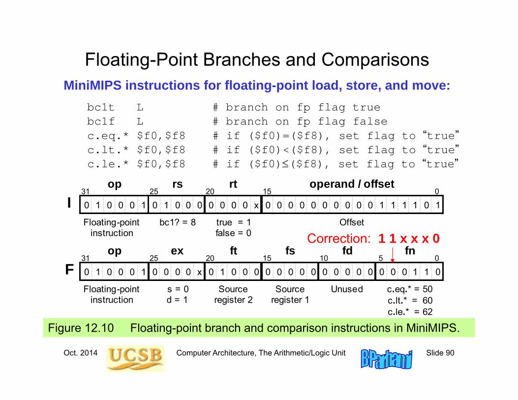
Floating-Point Branches and ComparisonsMiniMIPS instructions for floating-point load, store, and move:
bc1t L # branch on fp flag truebc1f L # branch on fp flag falsec.eq.* $f0,$f8 # if ($f0)=($f8), set flag to “true”c.lt.* $f0,$f8 # if ($f0)<($f8), set flag to “true”c.le.* $f0,$f8 # if ($f0)($f8), set flag to “true”
Figure 12.10 Floating-point branch and comparison instructions in MiniMIPS.
x
0 0 1 0 0 0 0 0 0 0 0 0 0 0 0 0 1 1 1 1 1 0 0 1 1 0 0 0 0 0 0 31 25 20 15 0
Floating-point instruction
true = 1 false = 0
bc1? = 8
Offset
op rs rt operand / offset
I
1 0 0 1 1 0 0 x 0 1 1 0 0 0 0 0 0 0 0 0 0 0 0 0 0 0 0 0 0 0 0 0 31 25 20 15 0
Floating-point instruction
s = 0 d = 1
Source register 2
op ex ft
F fs fd
10 5 fn
Unused c.eq.* = 50 c.lt.* = 60 c.le.* = 62
Source register 1
Correction: 1 1 x x x 0
Oct. 2014 Computer Architecture, The Arithmetic/Logic Unit Slide 91
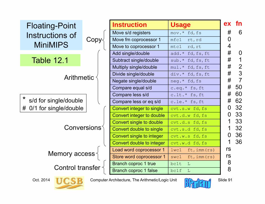
Floating-Point Instructions of
MiniMIPS
Instruction UsageMove s/d registers mov.* fd,fs
Move fm coprocessor 1 mfc1 rt,rd
Move to coprocessor 1 mtc1 rd,rt
Add single/double add.* fd,fs,ft
Subtract single/double sub.* fd,fs,ft
Multiply single/double mul.* fd,fs,ft
Divide single/double div.* fd,fs,ft
Negate single/double neg.* fd,fs
Compare equal s/d c.eq.* fs,ft
Compare less s/d c.lt.* fs,ft
Compare less or eq s/d c.le.* fs,ft
Convert integer to single cvt.s.w fd,fs
Convert integer to double cvt.d.w fd,fs
Convert single to double cvt.d.s fd,fs
Convert double to single cvt.s.d fd,fs
Convert single to integer cvt.w.s fd,fs
Convert double to integer cvt.w.d fd,fs
Load word coprocessor 1 lwc1 ft,imm(rs)
Store word coprocessor 1 swc1 ft,imm(rs)
Branch coproc 1 true bc1t L
Branch coproc 1 false bc1f L
Copy
Control transfer
Conversions
Arithmetic
Memory access
ex#04########001101rsrs88
fn6
01237
506062323333323636
Table 12.1
* s/d for single/double# 0/1 for single/double
Oct. 2014 Computer Architecture, The Arithmetic/Logic Unit Slide 92
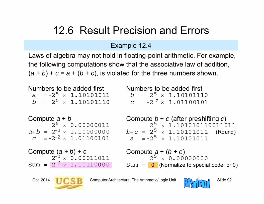
12.6 Result Precision and ErrorsExample 12.4
Laws of algebra may not hold in floating-point arithmetic. For example, the following computations show that the associative law of addition, (a + b) + c = a + (b + c), is violated for the three numbers shown.
Compute a + b 2 0.00000011a+b = 2 1.10000000 c =-2 1.01100101
Numbers to be added first a =-2 1.10101011 b = 2 1.10101110
5
5
Compute (a + b) + c 2 0.00011011Sum = 2 1.10110000
5
2 2
2 6
Compute b + c (after preshifting c) 2 1.101010110011011 b+c = 2 1.10101011 (Round) a =-2 1.10101011
Numbers to be added first b = 2 1.10101110 c =-2 1.01100101
5
5
Compute a + (b + c) 2 0.00000000 Sum = 0 (Normalize to special code for 0)
5 5
5
2

Oct. 2014 Computer Architecture, The Arithmetic/Logic Unit Slide 93
Error Control and Certifiable ArithmeticCatastrophic cancellation in subtracting almost equal numbers:
Area of a needlelike triangle
A = [s(s – a)(s – b)(s – c)]1/2
Possible remedies
Carry extra precision in intermediate results (guard digits):commonly used in calculators
Use alternate formula that does not produce cancellation errors
Certifiable arithmetic with intervals
A number is represented by its lower and upper bounds [xl, xu]
Example of arithmetic: [xl, xu] +interval [yl, yu] = [xl +fp yl, xu +fp yu]
ab c
Oct. 2014 Computer Architecture, The Arithmetic/Logic Unit Slide 94
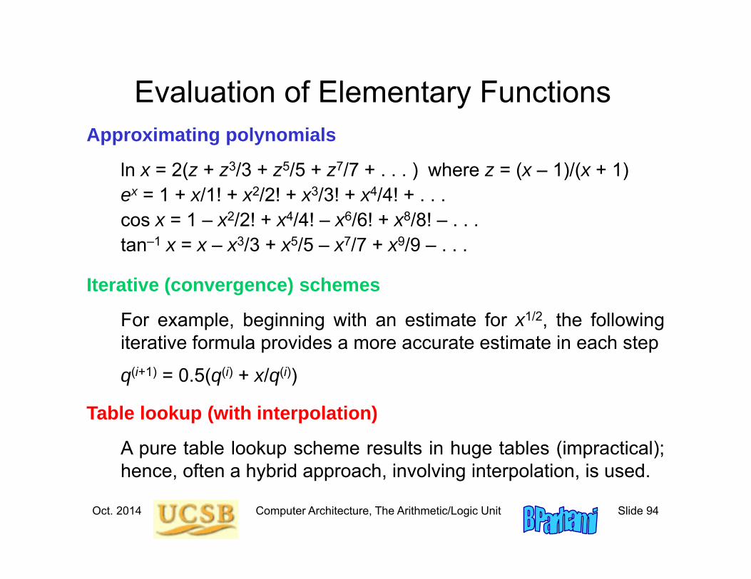
Evaluation of Elementary FunctionsApproximating polynomials
ln x = 2(z + z3/3 + z5/5 + z7/7 + . . . ) where z = (x – 1)/(x + 1)ex = 1 + x/1! + x2/2! + x3/3! + x4/4! + . . .cos x = 1 – x2/2! + x4/4! – x6/6! + x8/8! – . . .tan–1 x = x – x3/3 + x5/5 – x7/7 + x9/9 – . . .
Iterative (convergence) schemes
For example, beginning with an estimate for x1/2, the followingiterative formula provides a more accurate estimate in each step
q(i+1) = 0.5(q(i) + x/q(i))
Table lookup (with interpolation)
A pure table lookup scheme results in huge tables (impractical);hence, often a hybrid approach, involving interpolation, is used.
Oct. 2014 Computer Architecture, The Arithmetic/Logic Unit Slide 95
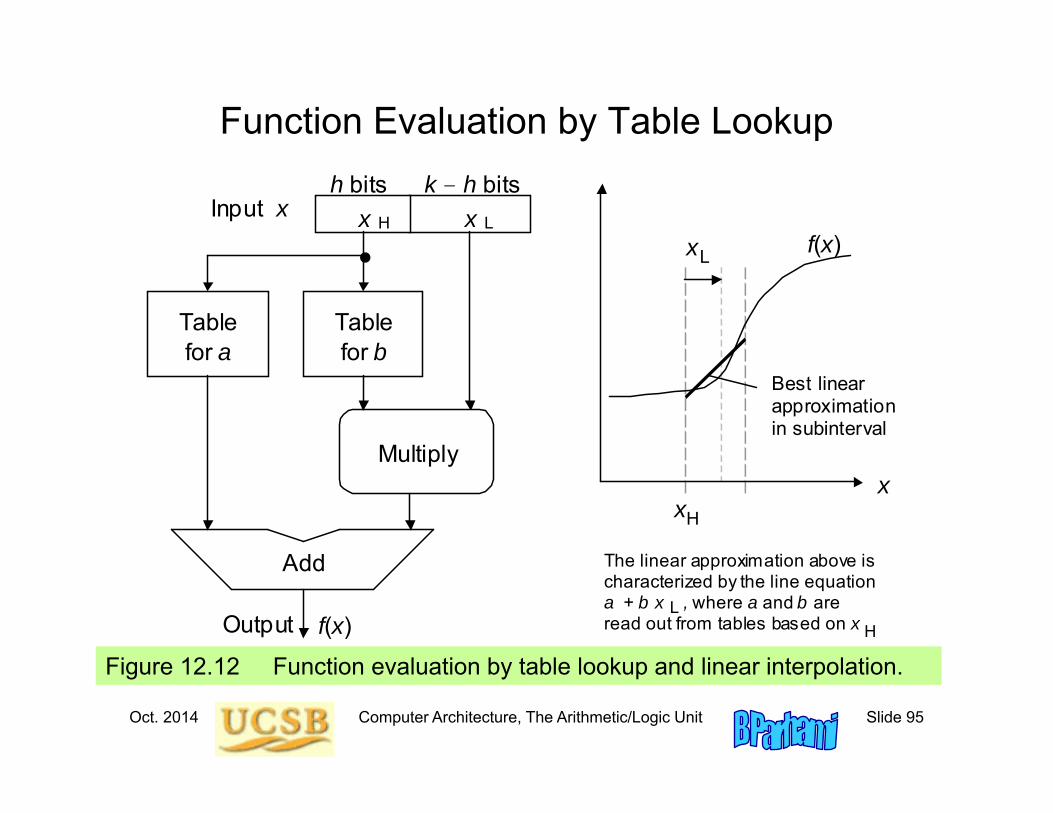
Figure 12.12 Function evaluation by table lookup and linear interpolation.
Function Evaluation by Table Lookup
L
Add
x
Table for a
Output
Table for b
x Input x H L
f(x)
Multiply
h bits k - h bits
x H
f(x) x
x
Best linear approximationin subinterval
The linear approximation above is characterized by the line equation a + b x , where a and b are read out from tables based on x
L H