Embed Size (px)
Citation preview
Computer Graphics (CS/ECE 545) Lecture 7: Morphology (Part 2) &Regions in Binary Images (Part 1)
Prof Emmanuel Agu
Computer Science Dept.Worcester Polytechnic Institute (WPI)
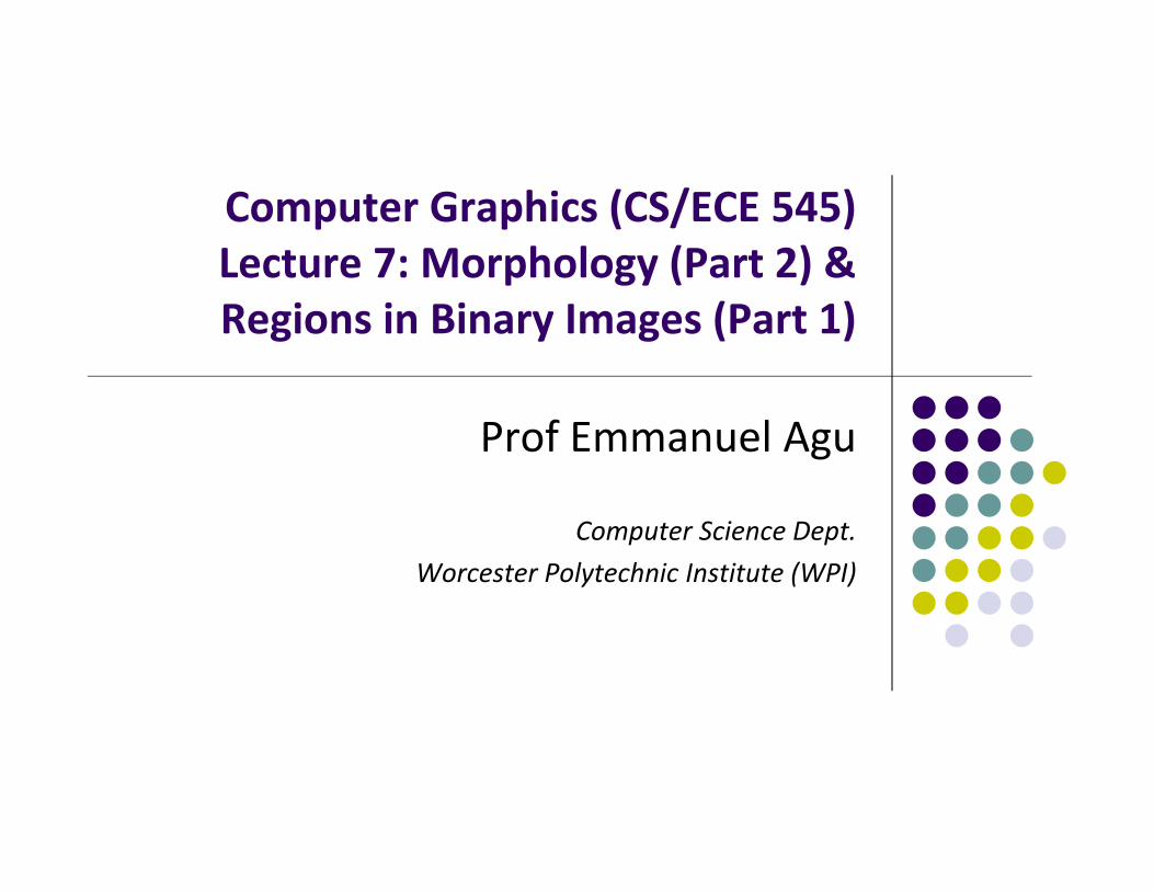
Recall: Dilation Example
For A and B shown below
Translation of A by (1,1)
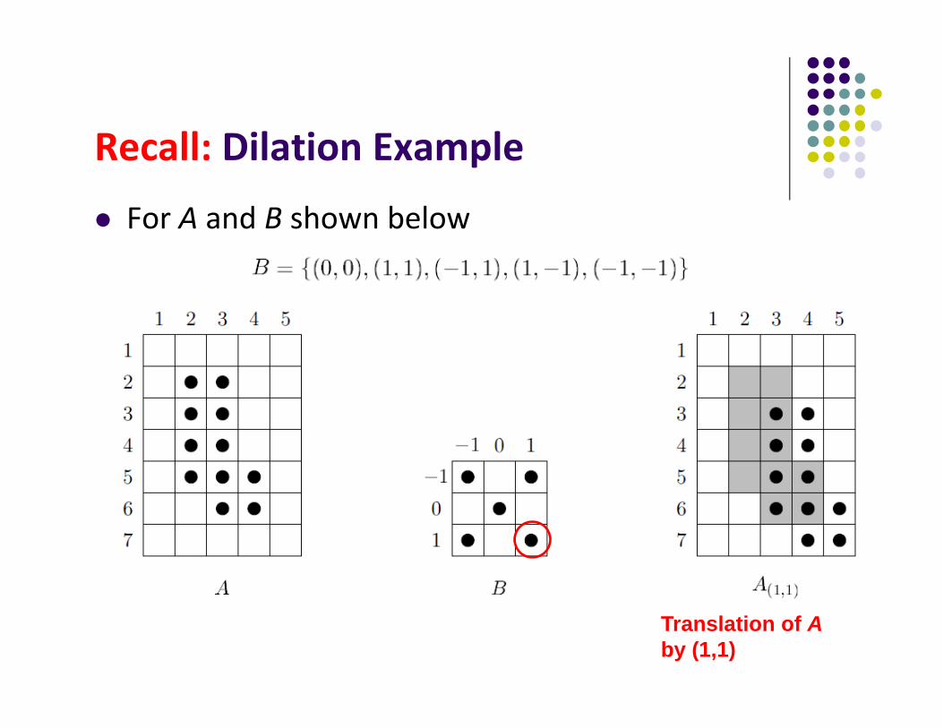
Recall: Dilation Example
Union of all translations
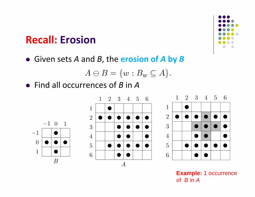
Recall: Erosion
Given sets A and B, the erosion of A by B
Find all occurrences of B in A
Example: 1 occurrence of B in A
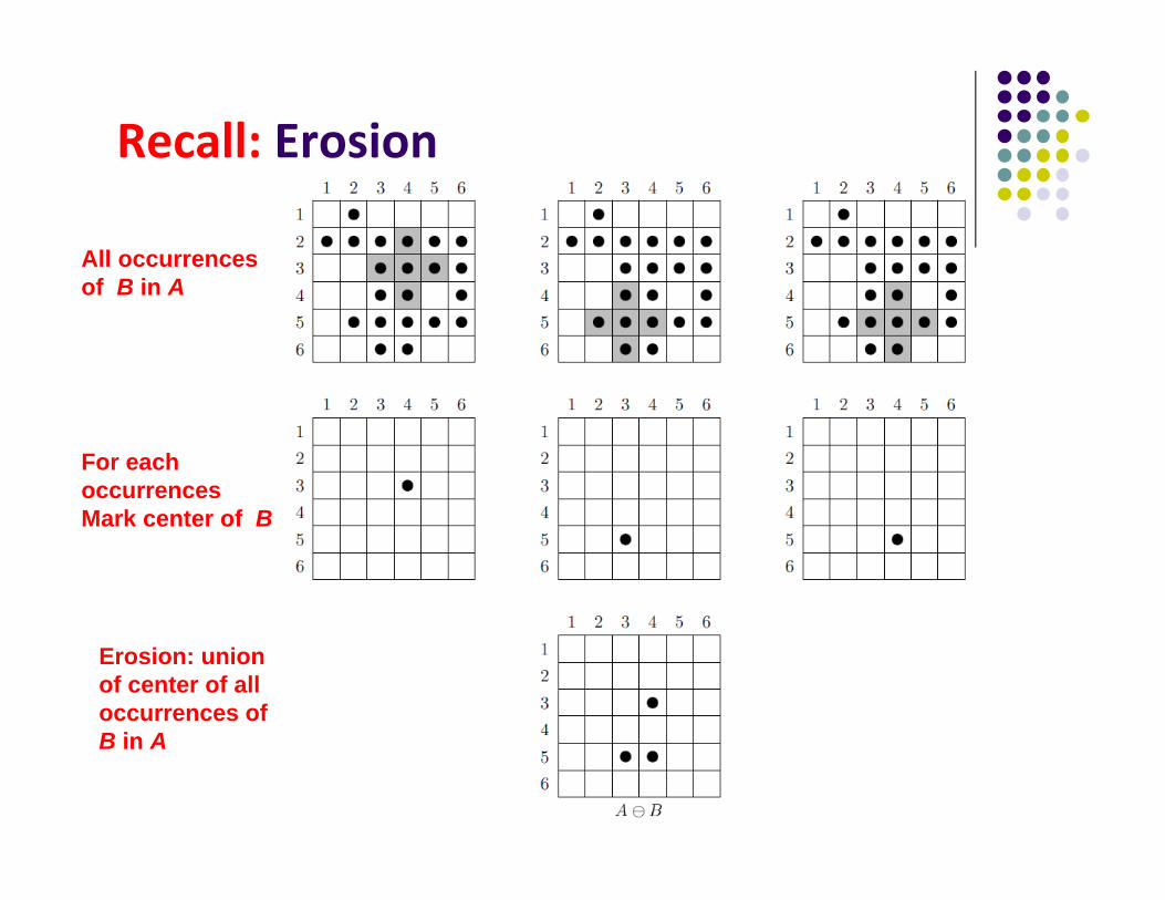
Recall: Erosion
All occurrencesof B in A
For each occurrencesMark center of B
Erosion: union of center of alloccurrences of B in A
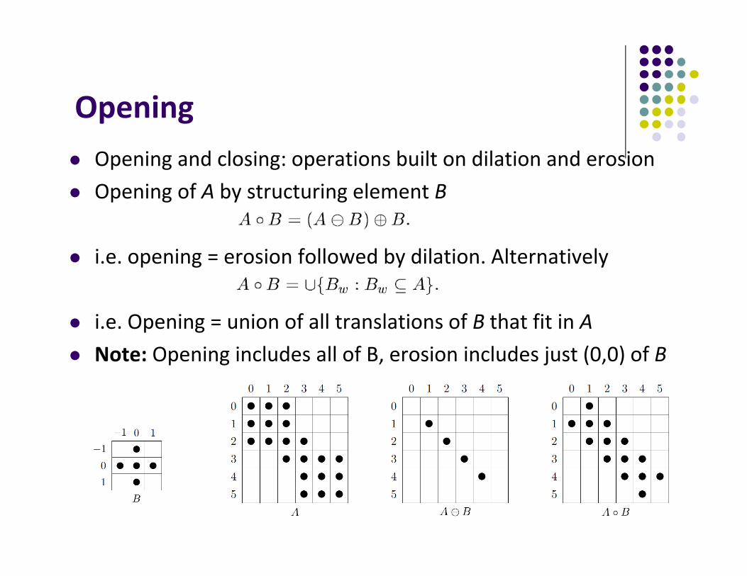
Opening Opening and closing: operations built on dilation and erosion Opening of A by structuring element B
i.e. opening = erosion followed by dilation. Alternatively
i.e. Opening = union of all translations of B that fit in A Note: Opening includes all of B, erosion includes just (0,0) of B
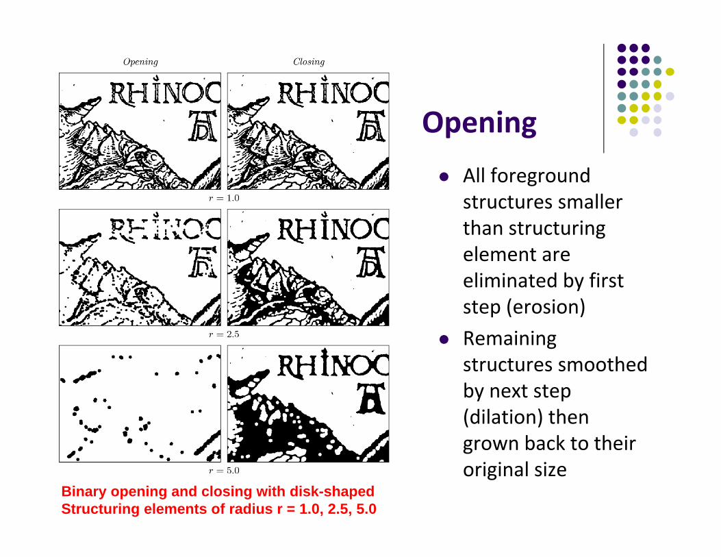
Opening All foreground
structures smaller than structuring element are eliminated by first step (erosion)
Remaining structures smoothed by next step (dilation) then grown back to their original size
Binary opening and closing with disk-shaped Structuring elements of radius r = 1.0, 2.5, 5.0
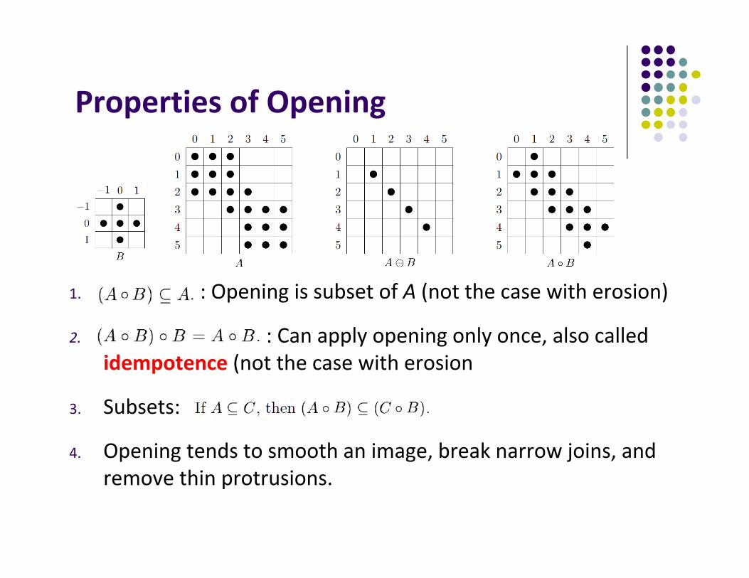
Properties of Opening
1. : Opening is subset of A (not the case with erosion)
2. : Can apply opening only once, also called idempotence (not the case with erosion
3. Subsets:
4. Opening tends to smooth an image, break narrow joins, and remove thin protrusions.
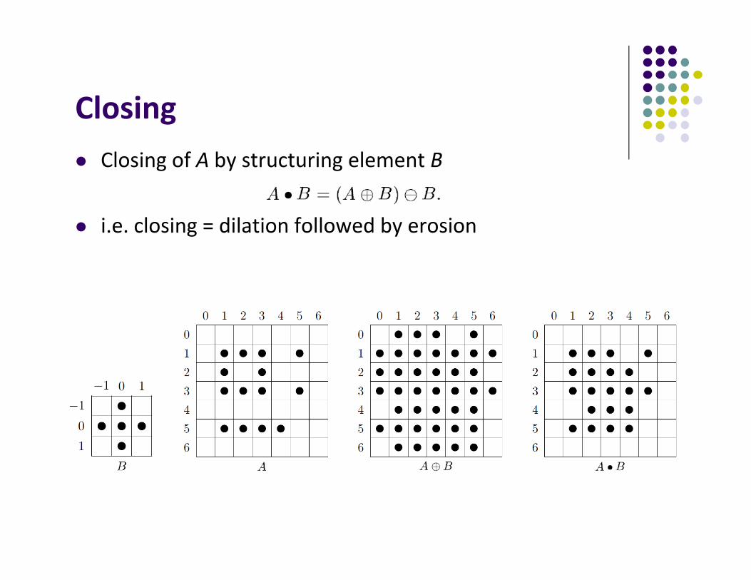
Closing Closing of A by structuring element B
i.e. closing = dilation followed by erosion
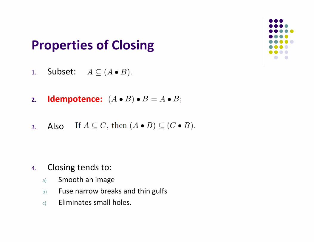
Properties of Closing
1. Subset:
2. Idempotence:
3. Also
4. Closing tends to:a) Smooth an imageb) Fuse narrow breaks and thin gulfs c) Eliminates small holes.
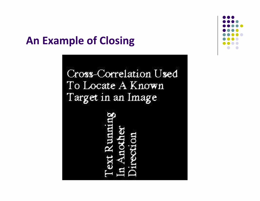
An Example of Closing
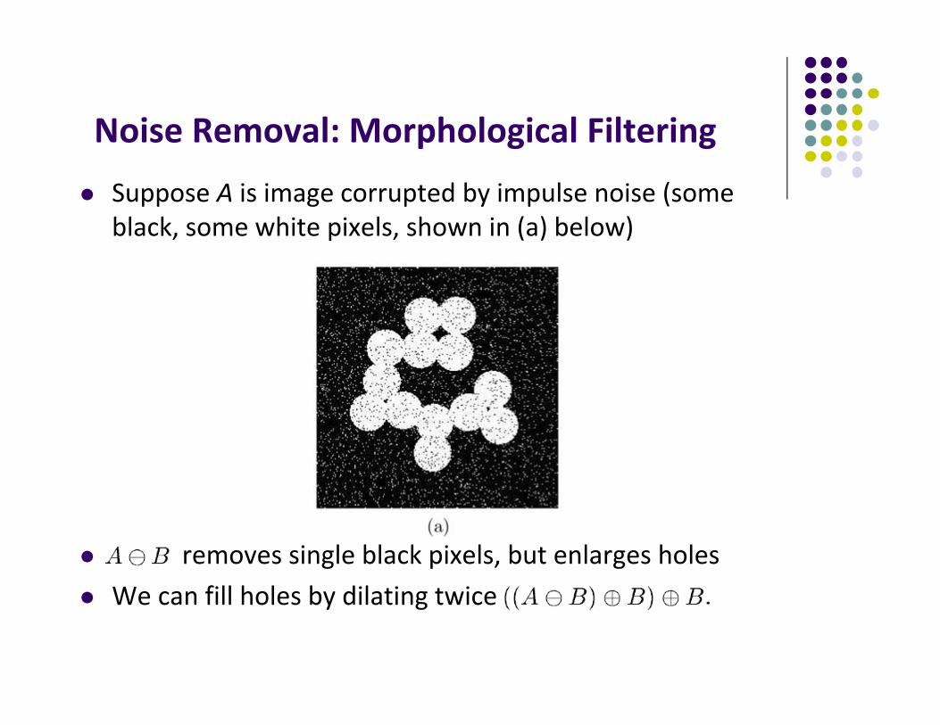
Noise Removal: Morphological Filtering
Suppose A is image corrupted by impulse noise (some black, some white pixels, shown in (a) below)
removes single black pixels, but enlarges holes We can fill holes by dilating twice
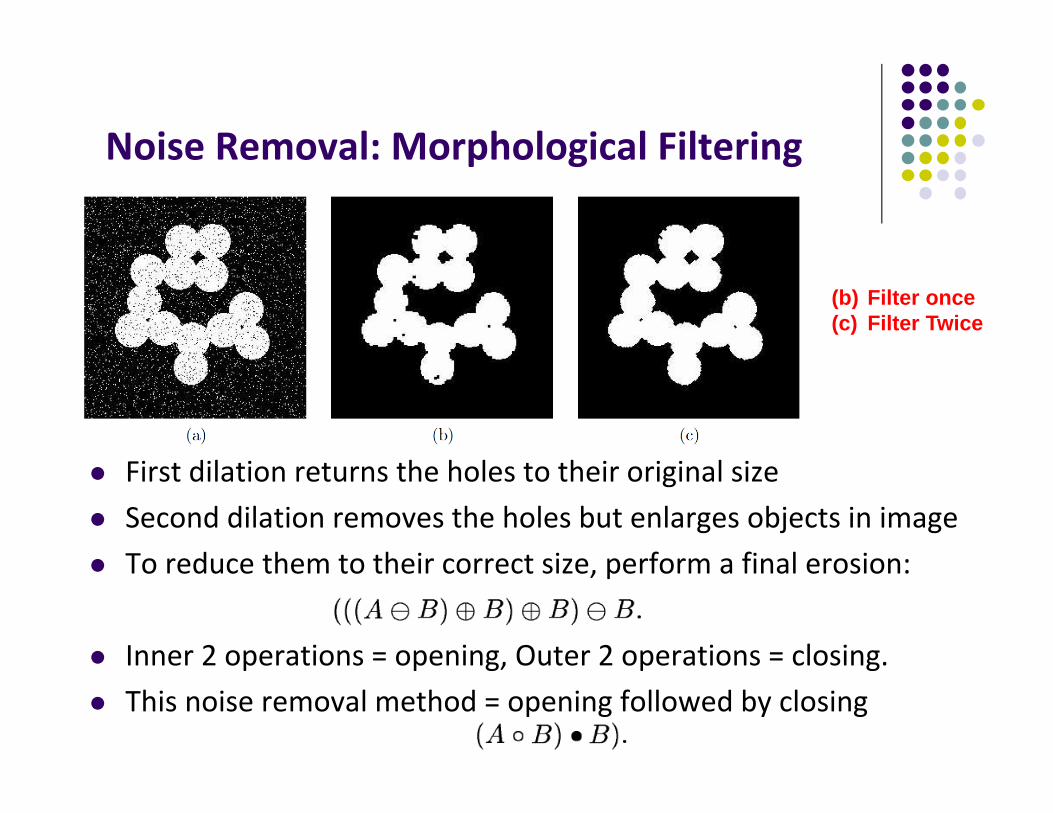
Noise Removal: Morphological Filtering
First dilation returns the holes to their original size Second dilation removes the holes but enlarges objects in image To reduce them to their correct size, perform a final erosion:
Inner 2 operations = opening, Outer 2 operations = closing. This noise removal method = opening followed by closing
(b) Filter once(c) Filter Twice
Relationship Between Opening and Closing
Opening and closing are duals i.e. Opening foreground = closing background, and vice versa
Complement of an opening = the closing of a complement
Complement of a closing = the opening of a complement.
Grayscale Morphology
Morphology operations can also be applied to grayscale images
Just replace (OR, AND) with (MAX, MIN) Consequently, morphology operations defined for
grayscale images can also operate on binary images (but not the other way around) ImageJ has single implementation of morphological operations that
works on binary and grayscale
For color images, perform grayscale morphology operations on each color channel (RGB)
For grayscale images, structuring element contains real values
Values may be –ve or 0
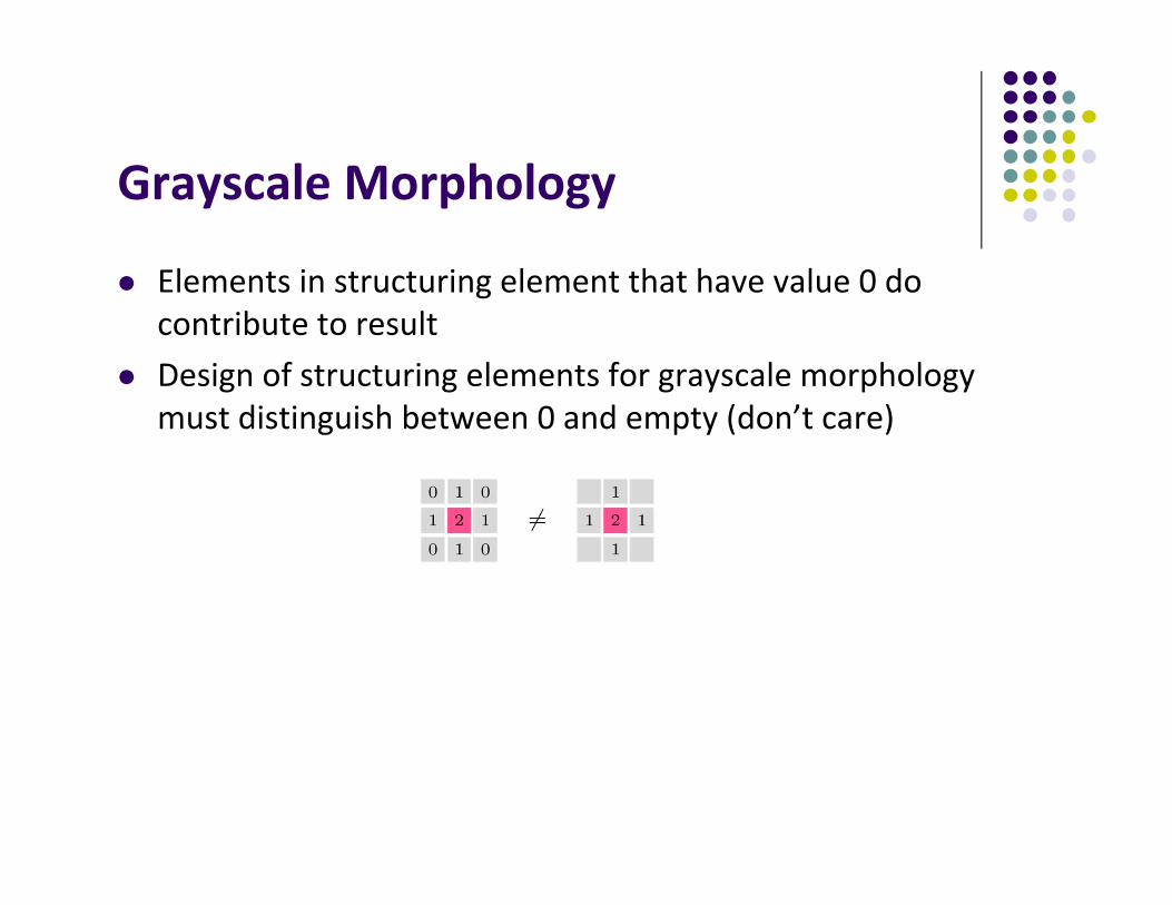
Grayscale Morphology
Elements in structuring element that have value 0 do contribute to result
Design of structuring elements for grayscale morphology must distinguish between 0 and empty (don’t care)
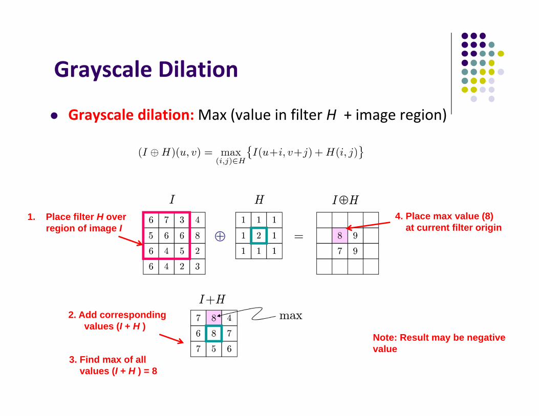
Grayscale Dilation
Grayscale dilation: Max (value in filter H + image region)
1. Place filter H over region of image I
2. Add correspondingvalues (I + H )
3. Find max of all values (I + H ) = 8
Note: Result may be negativevalue
4. Place max value (8)at current filter origin
Grayscale Erosion
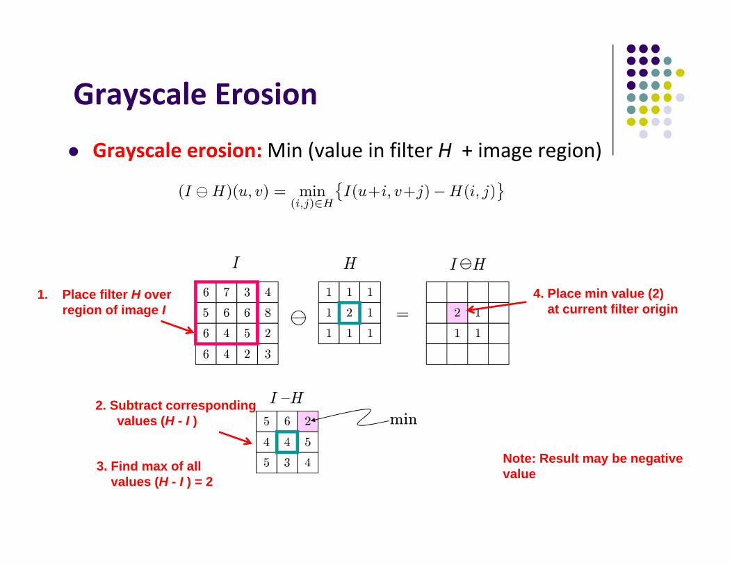
Grayscale erosion: Min (value in filter H + image region)
1. Place filter H over region of image I
2. Subtract correspondingvalues (H - I )
3. Find max of all values (H - I ) = 2
Note: Result may be negativevalue
4. Place min value (2)at current filter origin
Grayscale Opening and Closing
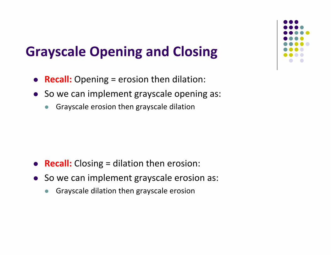
Recall: Opening = erosion then dilation: So we can implement grayscale opening as:
Grayscale erosion then grayscale dilation
Recall: Closing = dilation then erosion: So we can implement grayscale erosion as:
Grayscale dilation then grayscale erosion
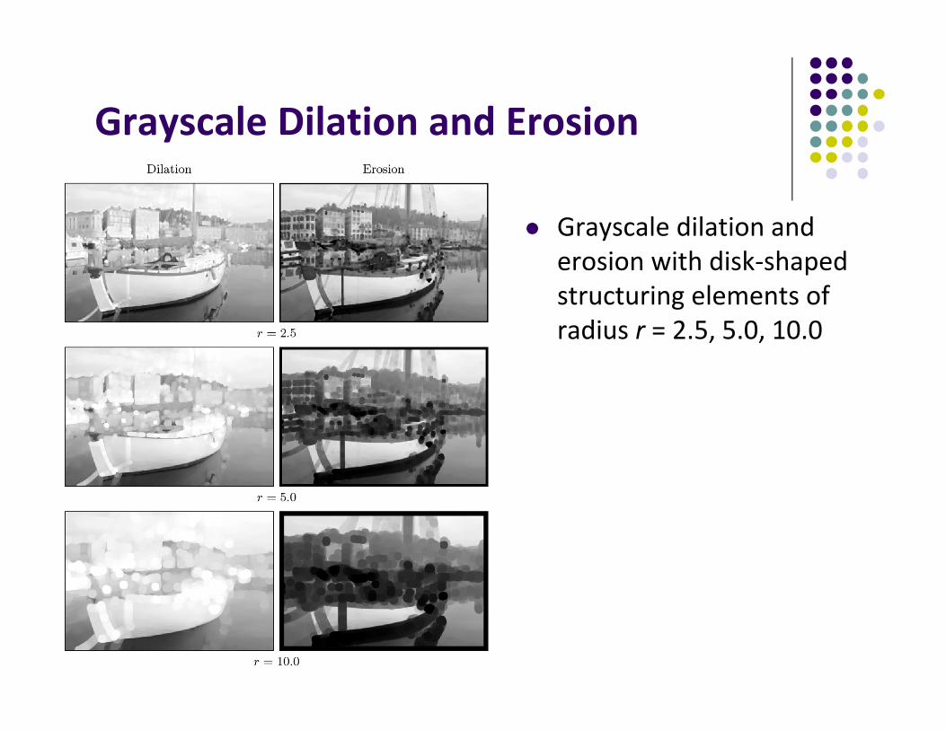
Grayscale Dilation and Erosion
Grayscale dilation and erosion with disk‐shaped structuring elements of radius r = 2.5, 5.0, 10.0
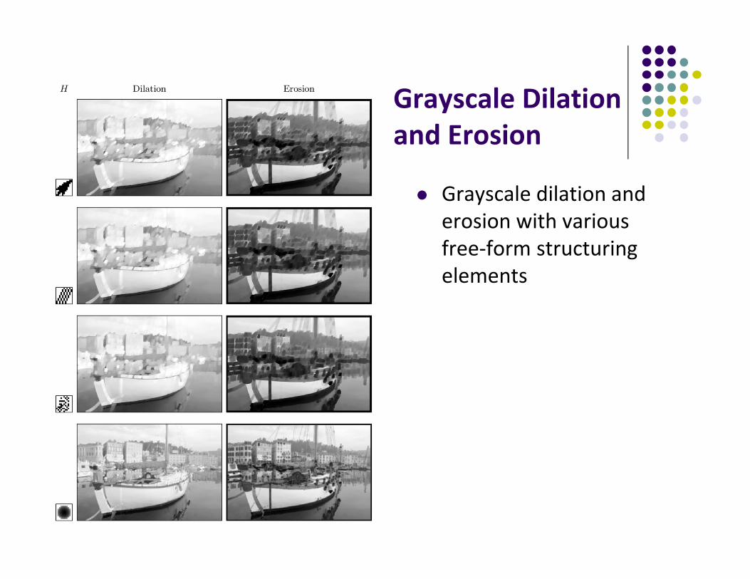
Grayscale Dilation and Erosion
Grayscale dilation and erosion with various free‐form structuring elements
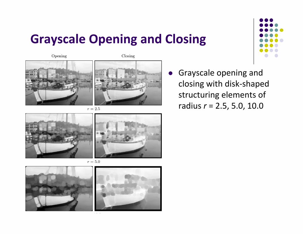
Grayscale Opening and Closing
Grayscale opening and closing with disk‐shaped structuring elements of radius r = 2.5, 5.0, 10.0
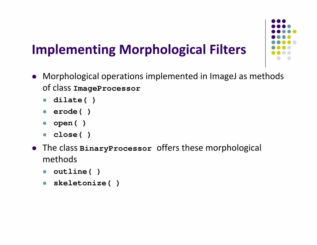
Implementing Morphological Filters
Morphological operations implemented in ImageJ as methods of class ImageProcessor dilate( ) erode( ) open( ) close( )
The class BinaryProcessor offers these morphological methods outline( ) skeletonize( )
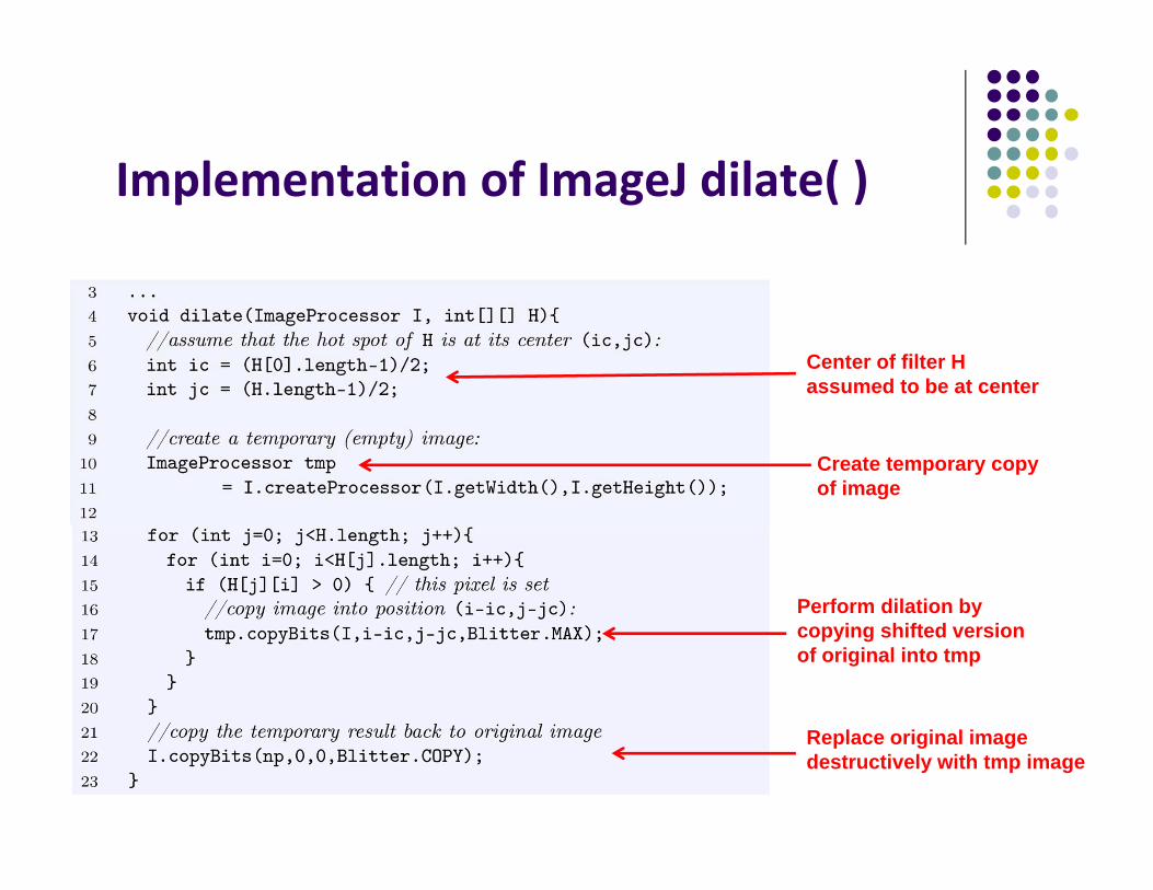
Implementation of ImageJ dilate( )
Center of filter H assumed to be at center
Create temporary copyof image
Perform dilation by copying shifted version of original into tmp
Replace original imagedestructively with tmp image
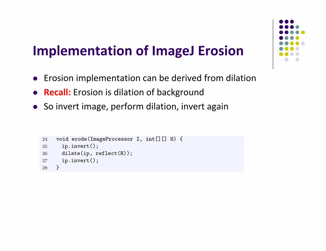
Implementation of ImageJ Erosion
Erosion implementation can be derived from dilation Recall: Erosion is dilation of background So invert image, perform dilation, invert again
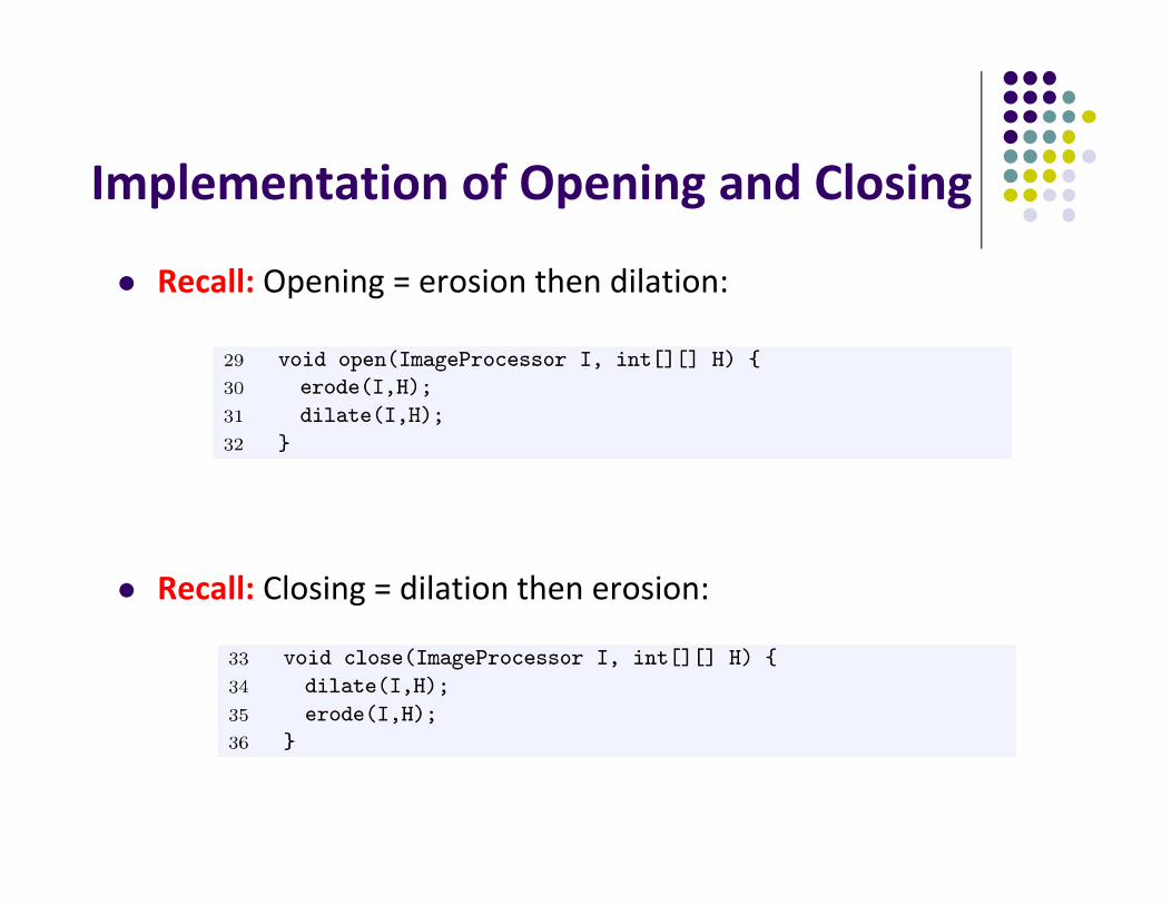
Implementation of Opening and Closing
Recall: Opening = erosion then dilation:
Recall: Closing = dilation then erosion:
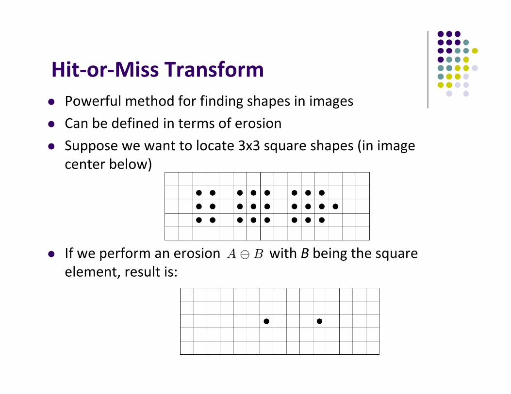
Hit‐or‐Miss Transform Powerful method for finding shapes in images Can be defined in terms of erosion Suppose we want to locate 3x3 square shapes (in image
center below)
If we perform an erosion with B being the square element, result is:
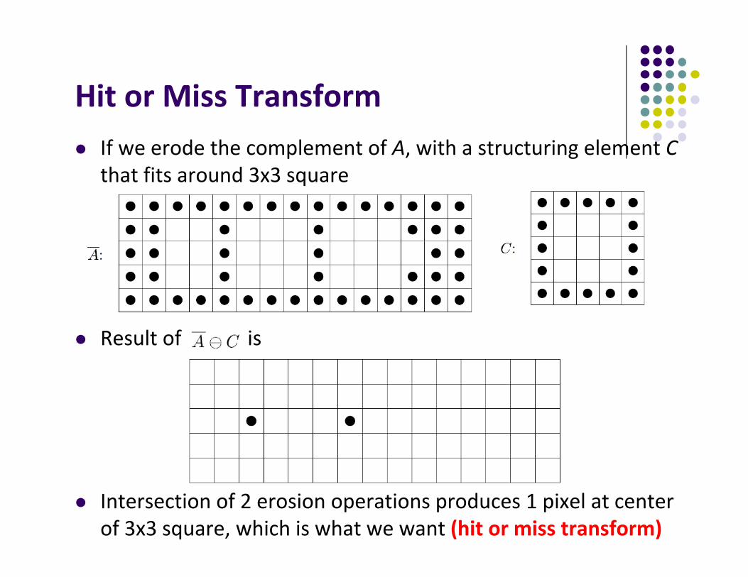
Hit or Miss Transform If we erode the complement of A, with a structuring element C
that fits around 3x3 square
Result of is
Intersection of 2 erosion operations produces 1 pixel at center of 3x3 square, which is what we want (hit or miss transform)
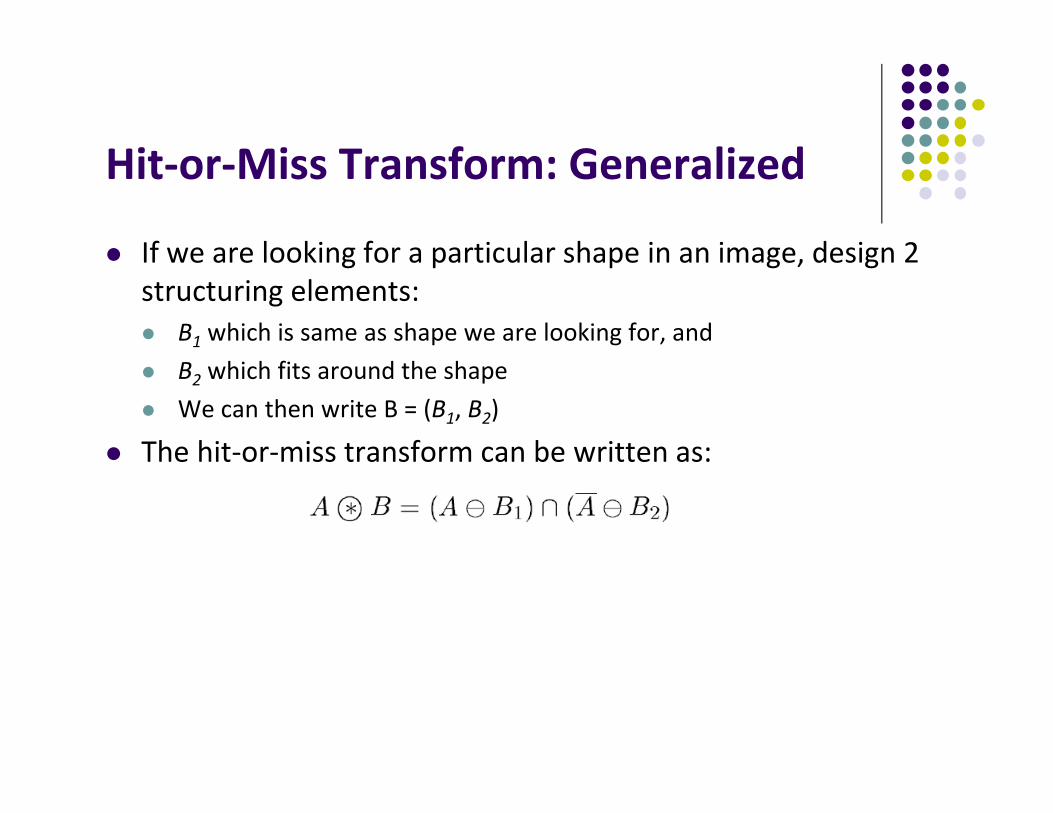
Hit‐or‐Miss Transform: Generalized
If we are looking for a particular shape in an image, design 2 structuring elements: B1 which is same as shape we are looking for, and B2 which fits around the shape We can then write B = (B1, B2)
The hit‐or‐miss transform can be written as:
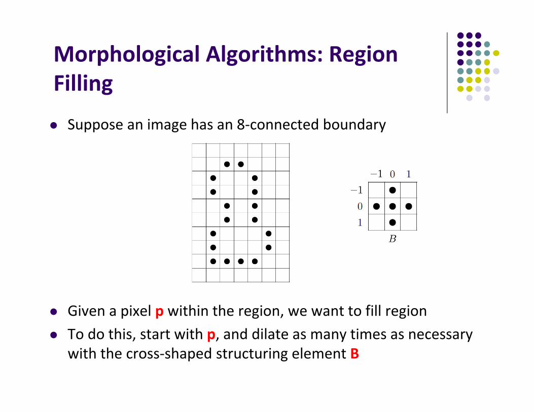
Morphological Algorithms: Region Filling
Suppose an image has an 8‐connected boundary
Given a pixel p within the region, we want to fill region To do this, start with p, and dilate as many times as necessary
with the cross‐shaped structuring element B
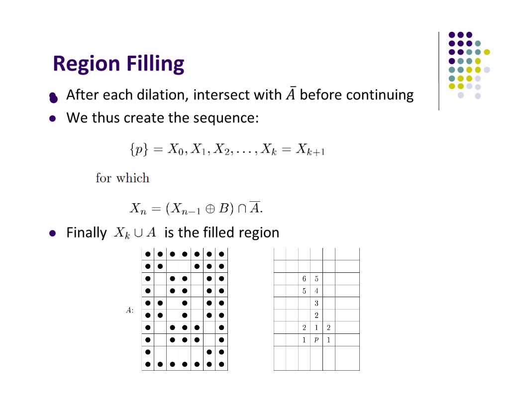
Region Filling
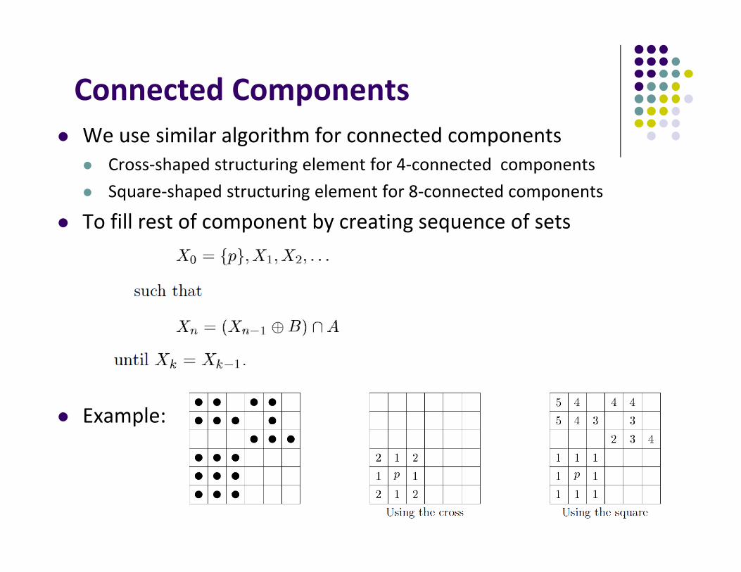
Connected Components We use similar algorithm for connected components
Cross‐shaped structuring element for 4‐connected components Square‐shaped structuring element for 8‐connected components
To fill rest of component by creating sequence of sets
Example:
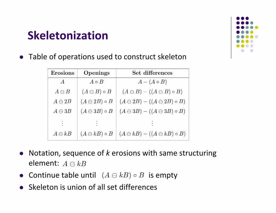
Skeletonization
Table of operations used to construct skeleton
Notation, sequence of k erosions with same structuring element:
Continue table until is empty Skeleton is union of all set differences
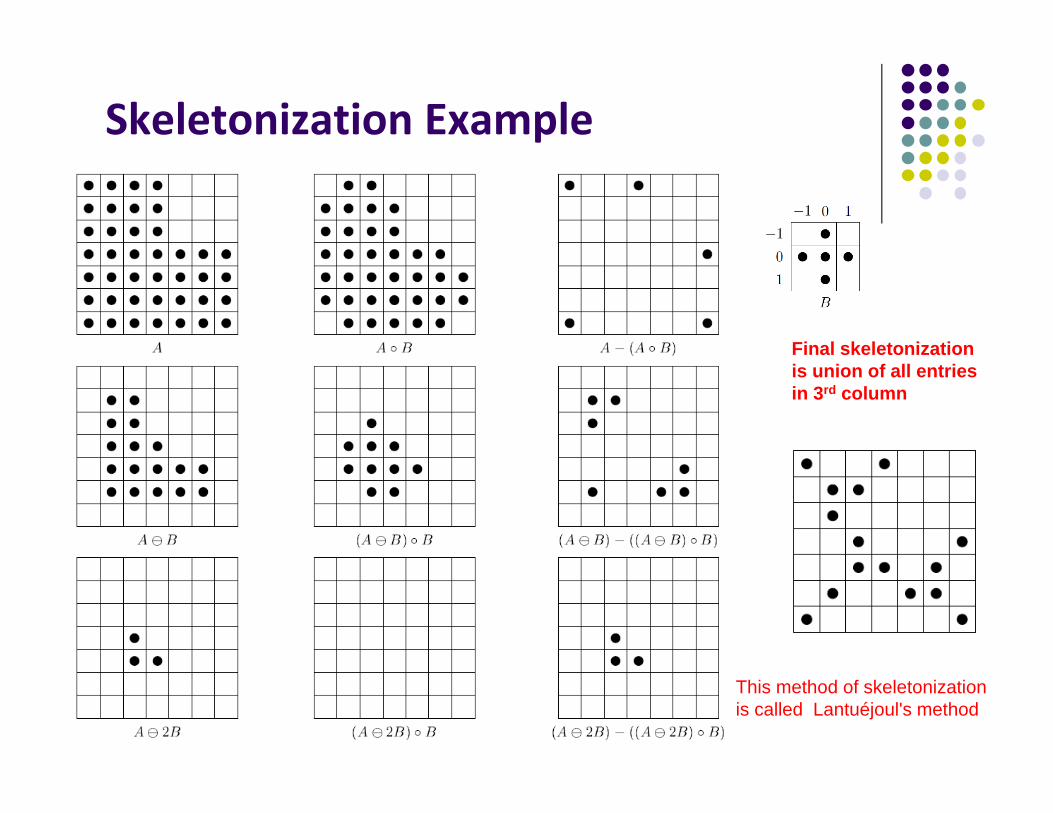
Skeletonization Example
d
Final skeletonization is union of all entries in 3rd column
This method of skeletonization is called Lantuéjoul's method
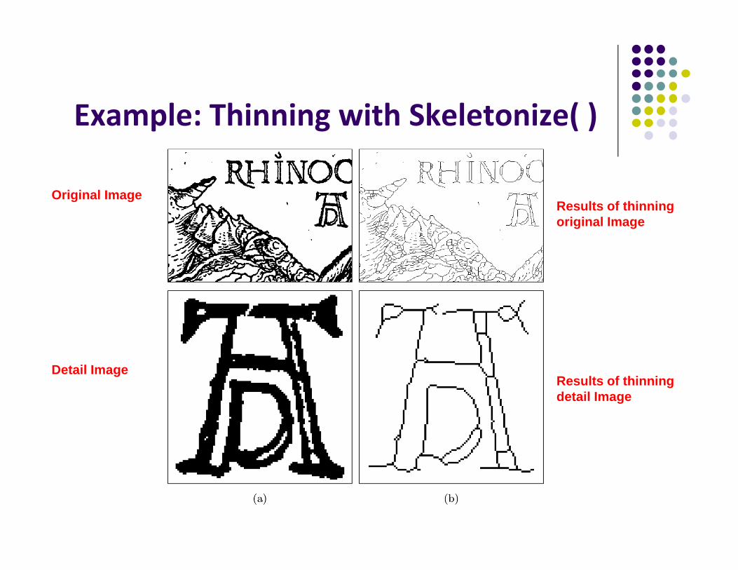
Example: Thinning with Skeletonize( )
Original Image
Detail ImageResults of thinning detail Image
Results of thinning original Image
References Wilhelm Burger and Mark J. Burge, Digital Image Processing, Springer, 2008
Rutgers University, CS 334, Introduction to Imaging and Multimedia, Fall 2012
Alasdair McAndrews, Introduction to Digital Image Processing with MATLAB, 2004
Computer Graphics (CS/ECE 545) Lecture 7:
Regions in Binary Images (Part 1)
Prof Emmanuel Agu
Computer Science Dept.Worcester Polytechnic Institute (WPI)
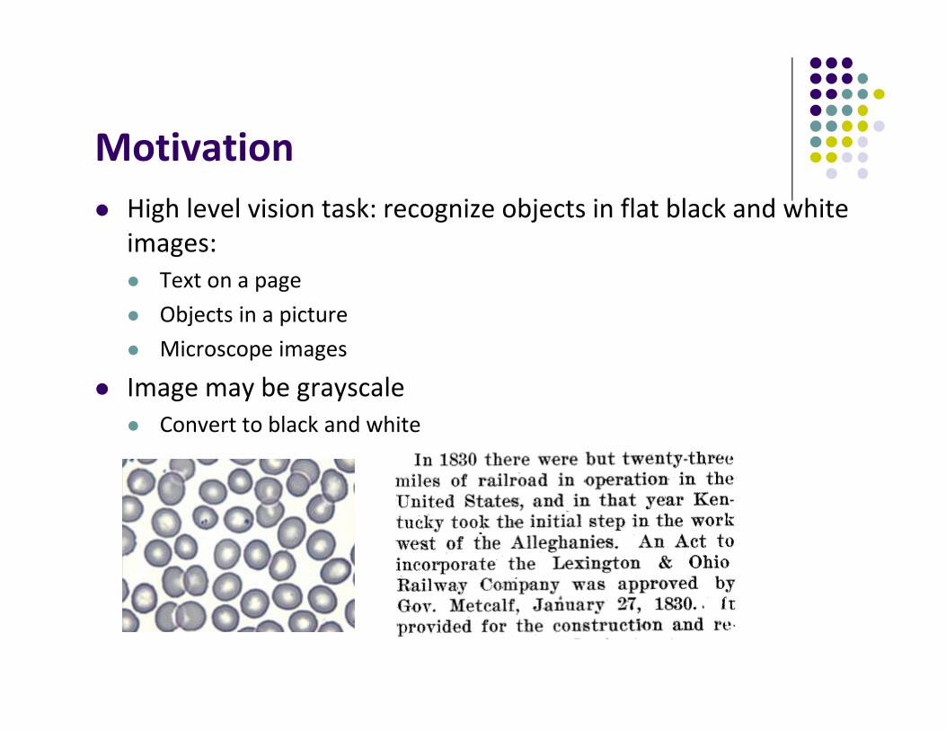
Motivation High level vision task: recognize objects in flat black and white
images: Text on a page Objects in a picture Microscope images
Image may be grayscale Convert to black and white
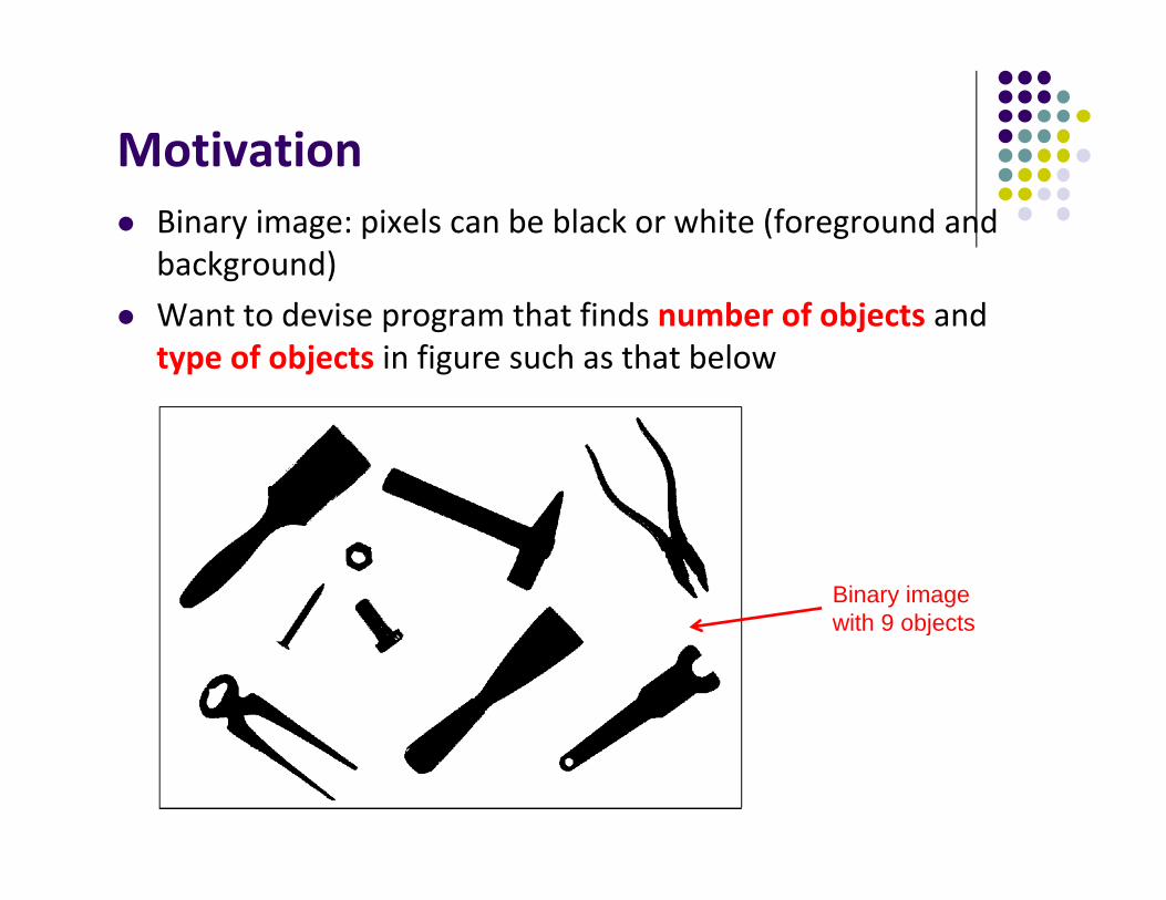
Motivation Binary image: pixels can be black or white (foreground and
background) Want to devise program that finds number of objects and
type of objects in figure such as that below
Binary imagewith 9 objects
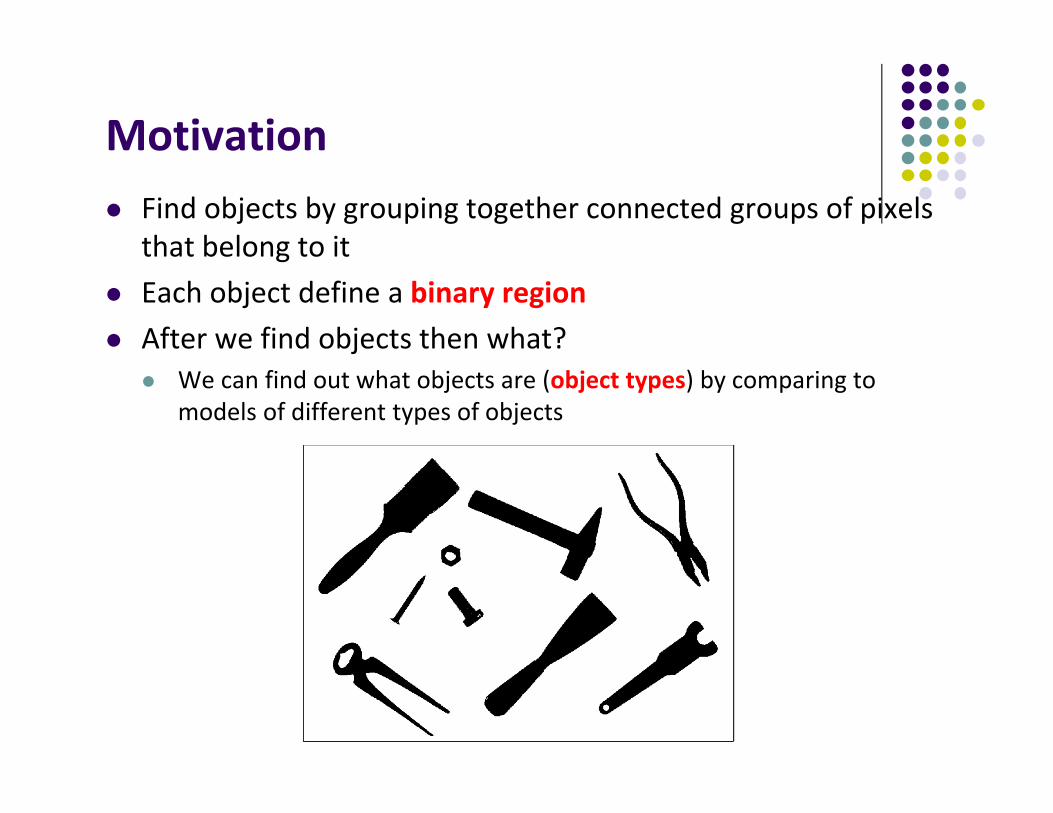
Motivation Find objects by grouping together connected groups of pixels
that belong to it Each object define a binary region After we find objects then what?
We can find out what objects are (object types) by comparing to models of different types of objects
Finding Image Regions
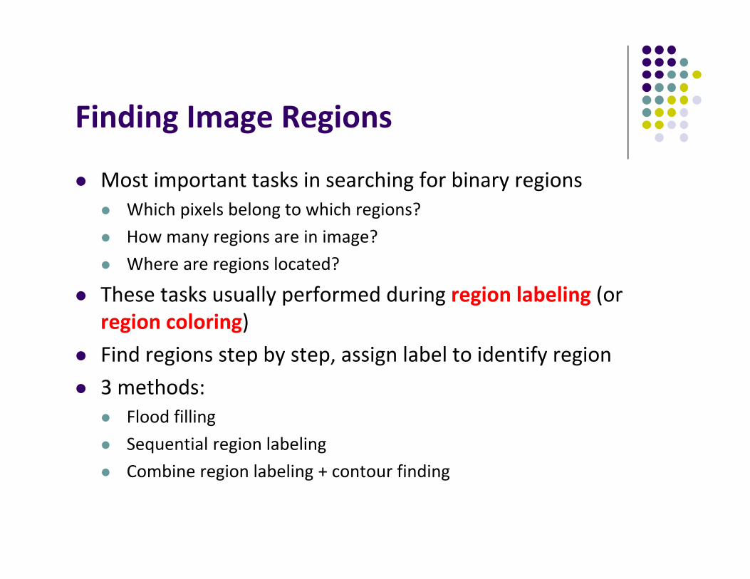
Most important tasks in searching for binary regions Which pixels belong to which regions? How many regions are in image? Where are regions located?
These tasks usually performed during region labeling (or region coloring)
Find regions step by step, assign label to identify region 3 methods:
Flood filling Sequential region labeling Combine region labeling + contour finding
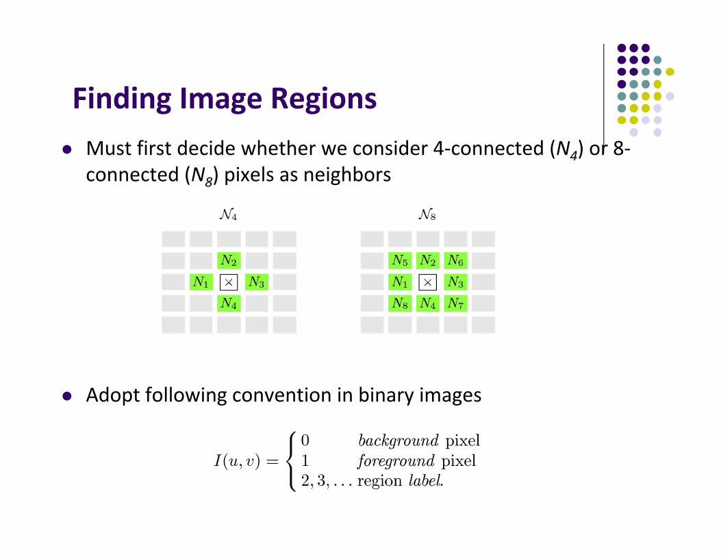
Finding Image Regions Must first decide whether we consider 4‐connected (N4) or 8‐
connected (N8) pixels as neighbors
Adopt following convention in binary images
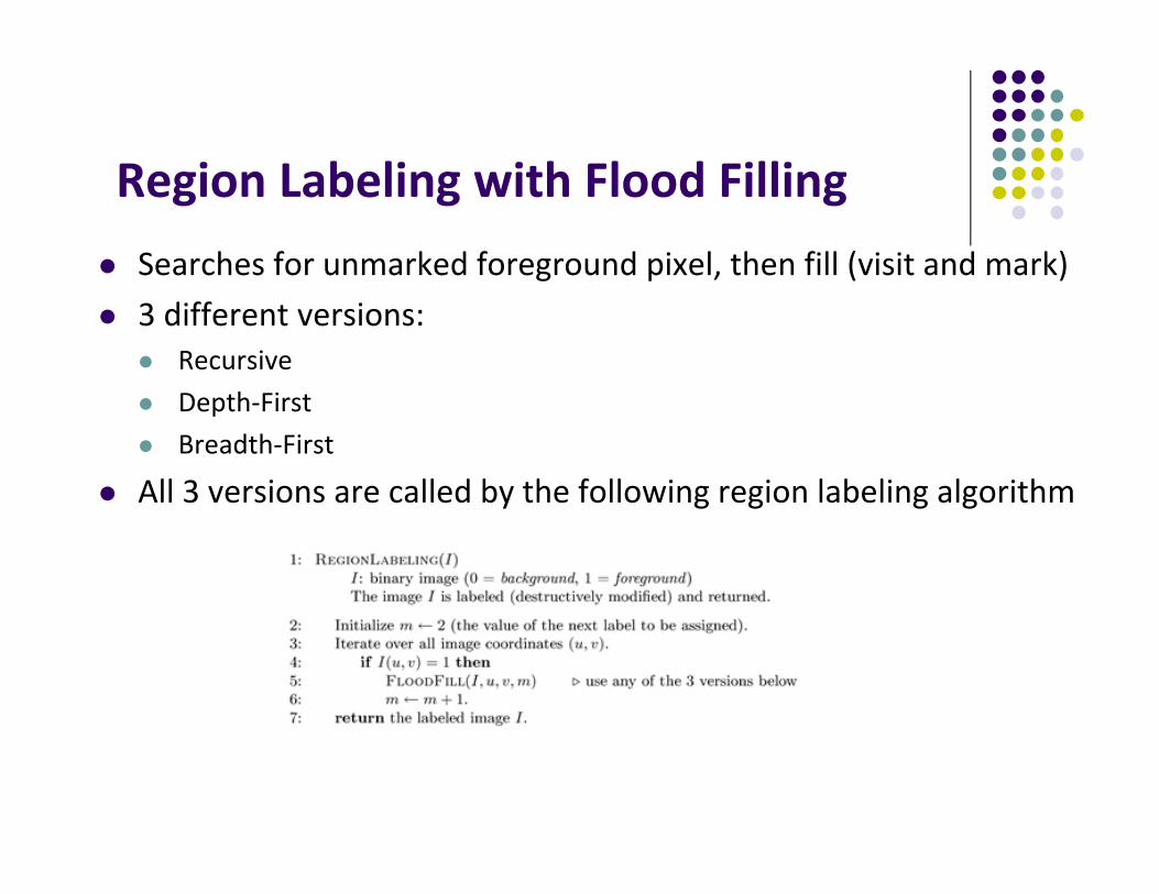
Region Labeling with Flood Filling Searches for unmarked foreground pixel, then fill (visit and mark) 3 different versions:
Recursive Depth‐First Breadth‐First
All 3 versions are called by the following region labeling algorithm
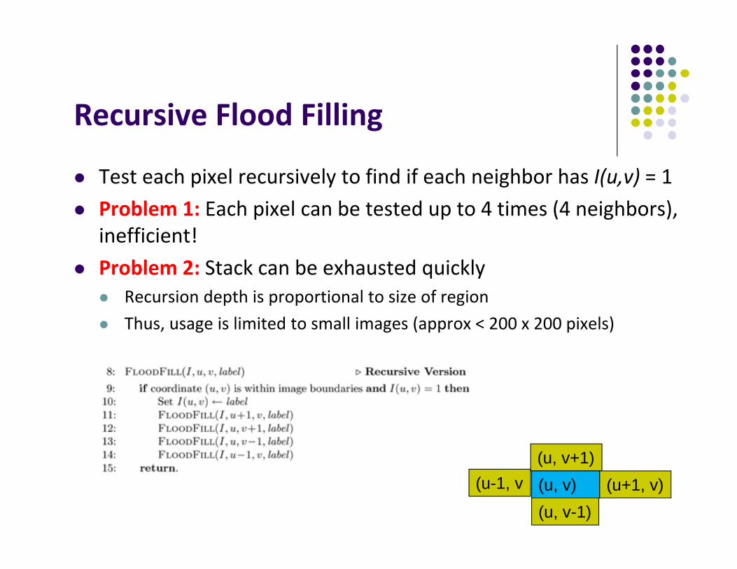
Recursive Flood Filling
Test each pixel recursively to find if each neighbor has I(u,v) = 1 Problem 1: Each pixel can be tested up to 4 times (4 neighbors),
inefficient! Problem 2: Stack can be exhausted quickly
Recursion depth is proportional to size of region Thus, usage is limited to small images (approx < 200 x 200 pixels)
(u, v+1)(u, v)(u, v-1)
(u+1, v)(u-1, v
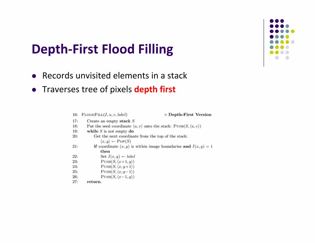
Depth‐First Flood Filling
Records unvisited elements in a stack Traverses tree of pixels depth first
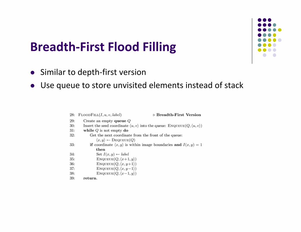
Breadth‐First Flood Filling
Similar to depth‐first version Use queue to store unvisited elements instead of stack
Depth‐First Flood‐Filling
Let’s look at an implementation of depth‐first flood filling A run: group of adjacent pixels lying on same scanline Fill runs(adjacent, on same scan line) of pixels
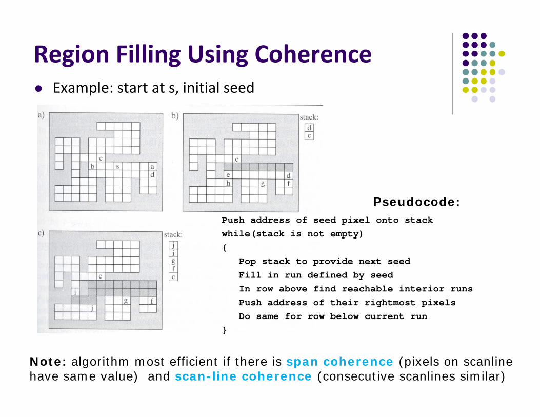
Region Filling Using Coherence Example: start at s, initial seed
Push address of seed pixel onto stackwhile(stack is not empty){
Pop stack to provide next seedFill in run defined by seedIn row above find reachable interior runsPush address of their rightmost pixelsDo same for row below current run
}
Note: algorithm most efficient if there is span coherence (pixels on scanline have same value) and scan-line coherence (consecutive scanlines similar)
Pseudocode:
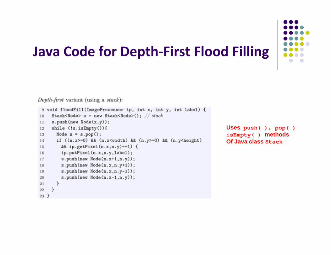
Java Code for Depth‐First Flood Filling
Uses push( ), pop( )isEmpty( ) methods Of Java class Stack
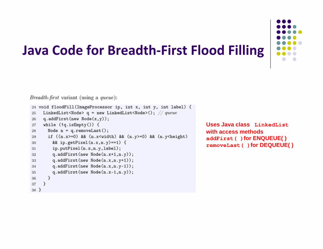
Java Code for Breadth‐First Flood Filling
Uses Java class LinkedList with access methods addFirst( )for ENQUEUE( )removeLast( )for DEQUEUE( )
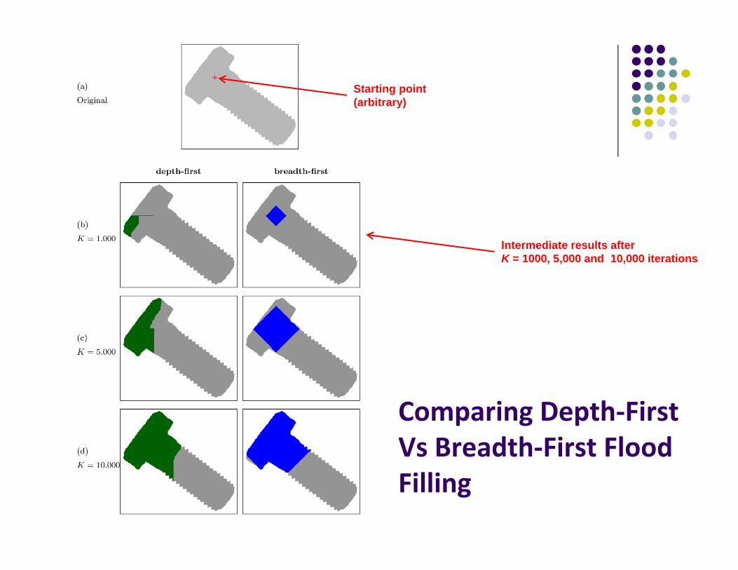
Comparing Depth‐First Vs Breadth‐First Flood Filling
Starting point(arbitrary)
Intermediate results after K = 1000, 5,000 and 10,000 iterations
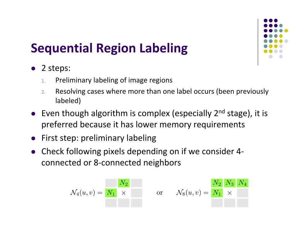
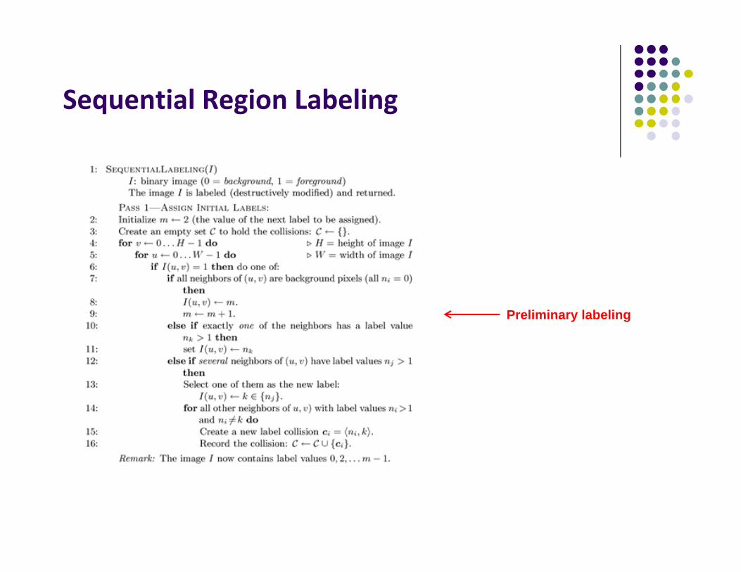
Sequential Region Labeling 2 steps:
1. Preliminary labeling of image regions2. Resolving cases where more than one label occurs (been previously
labeled)
Even though algorithm is complex (especially 2nd stage), it is preferred because it has lower memory requirements
First step: preliminary labeling Check following pixels depending on if we consider 4‐
connected or 8‐connected neighbors
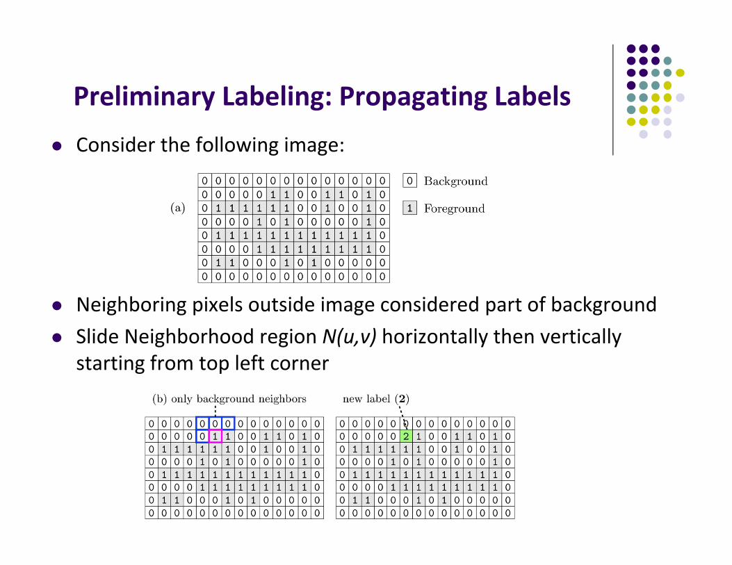
Preliminary Labeling: Propagating Labels
Consider the following image:
Neighboring pixels outside image considered part of background Slide Neighborhood region N(u,v) horizontally then vertically
starting from top left corner
Preliminary Labeling: Propagating Labels
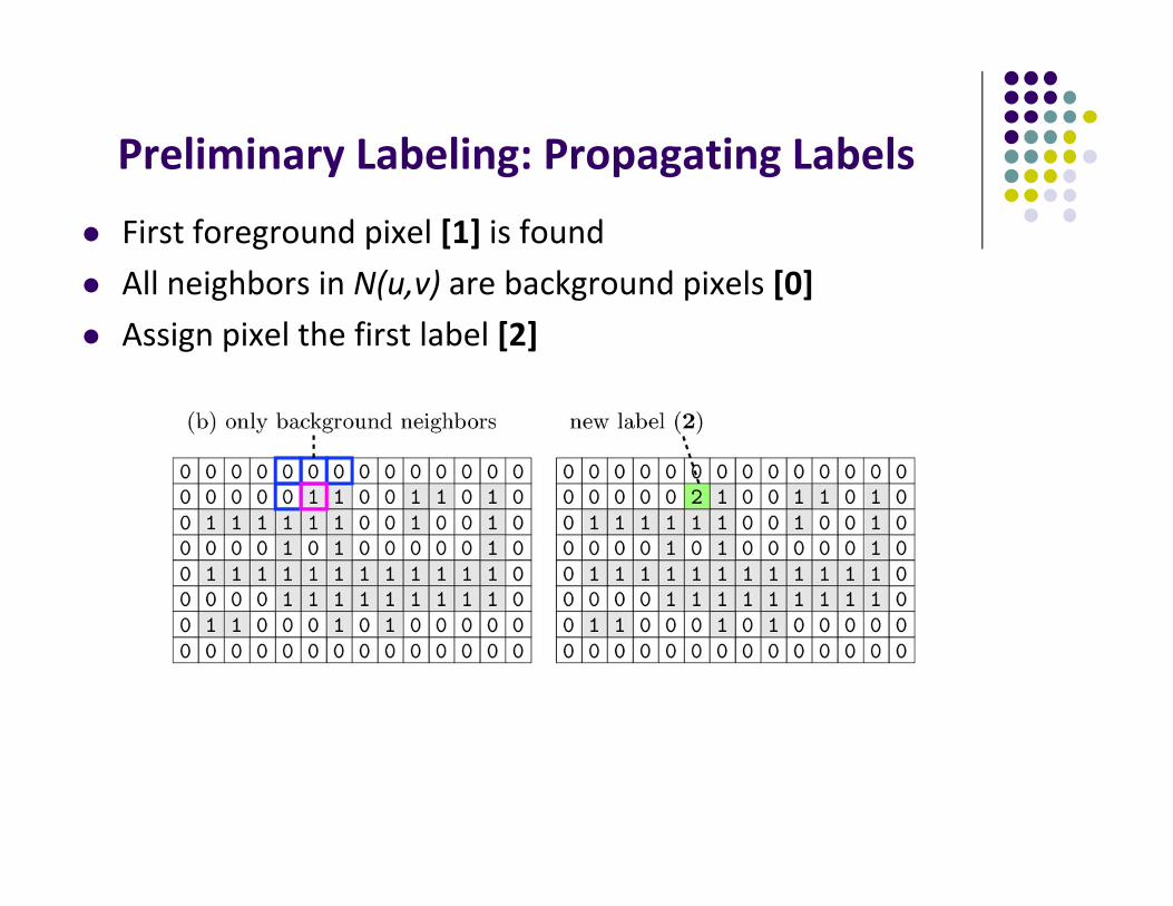
First foreground pixel [1] is found All neighbors in N(u,v) are background pixels [0] Assign pixel the first label [2]
Preliminary Labeling: Propagating Labels
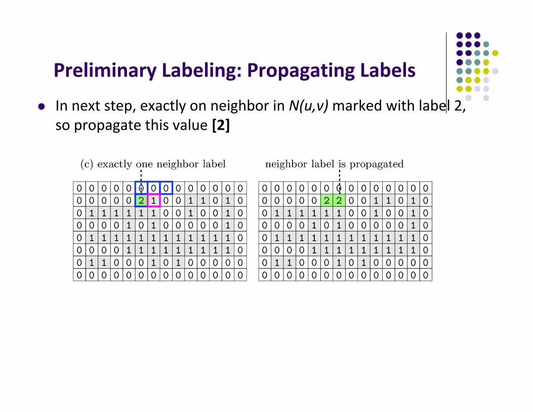
In next step, exactly on neighbor in N(u,v) marked with label 2, so propagate this value [2]
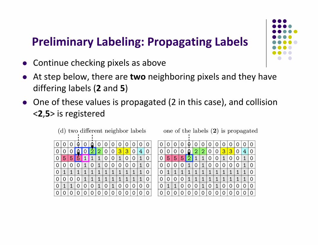
Preliminary Labeling: Propagating Labels
Continue checking pixels as above At step below, there are two neighboring pixels and they have
differing labels (2 and 5) One of these values is propagated (2 in this case), and collision
<2,5> is registered
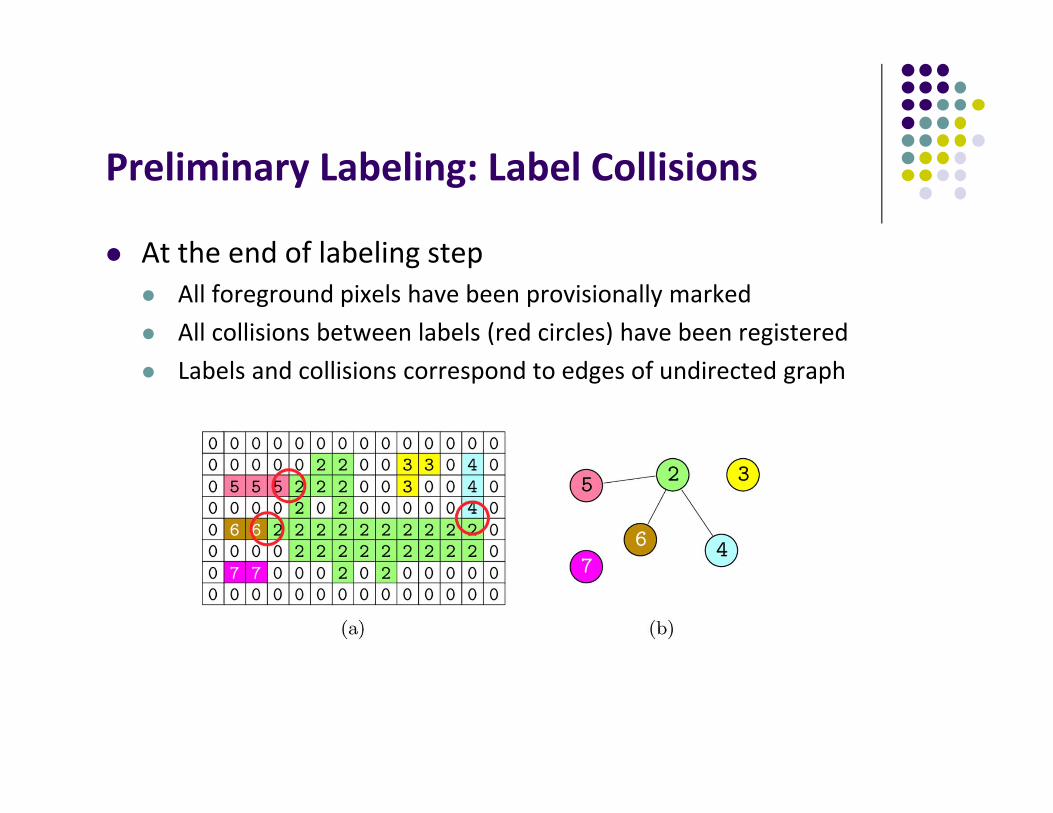
Preliminary Labeling: Label Collisions
At the end of labeling step All foreground pixels have been provisionally marked All collisions between labels (red circles) have been registered Labels and collisions correspond to edges of undirected graph
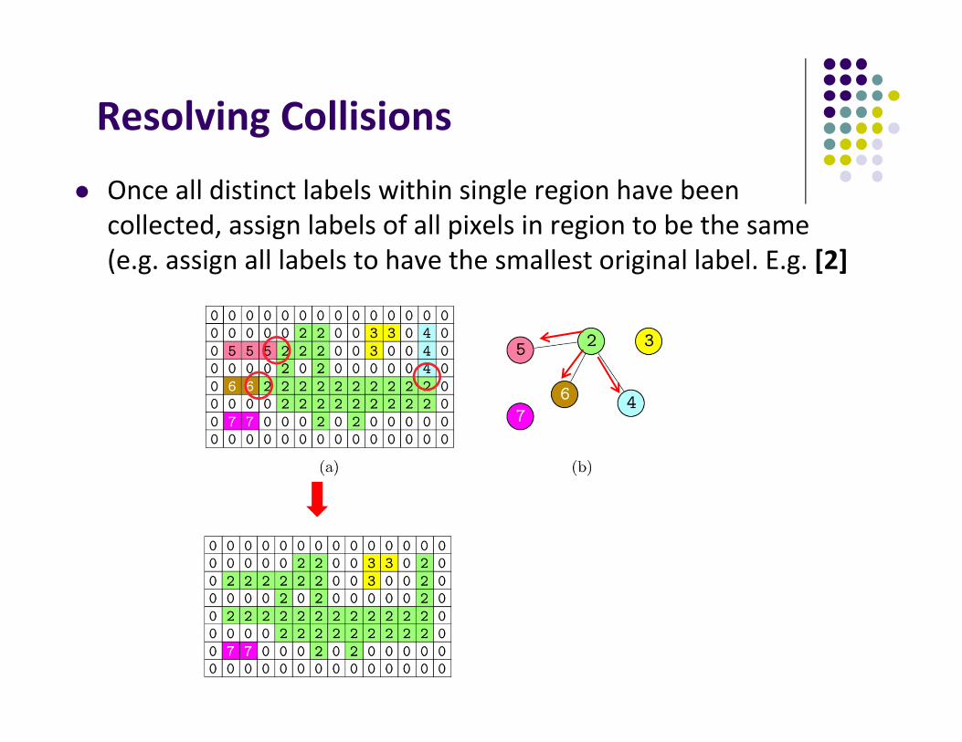
Resolving Collisions
Once all distinct labels within single region have been collected, assign labels of all pixels in region to be the same (e.g. assign all labels to have the smallest original label. E.g. [2]
Sequential Region Labeling
Preliminary labeling
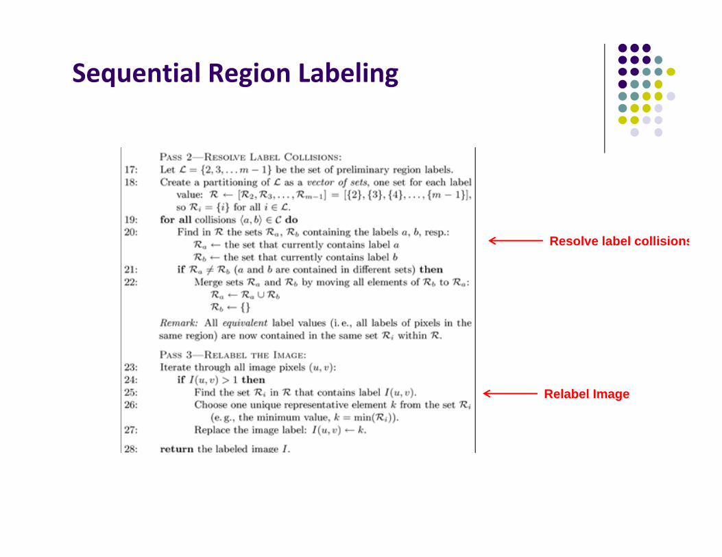
Sequential Region Labeling
Resolve label collisions
Relabel Image
References Wilhelm Burger and Mark J. Burge, Digital Image Processing, Springer, 2008
Rutgers University, CS 334, Introduction to Imaging and Multimedia, Fall 2012