Computing Most Probable Worlds for Action Probabilistic ...€¦ · Computing Most Probable Worlds for Action Probabilistic Logic Programs ... naive algorithm to solve the MPW problem

Computing Most Probable Worldsfor Action Probabilistic Logic Programs †

Gerardo Ignacio [email protected]

Department of Computer ScienceUniversity of Maryland College Park

Abstract

The semantics of probabilistic logic programs (PLPs) is usually given through a possibleworlds semantics. We propose a variant of PLPs called action probabilistic logic programs orap-programs that use a two-sorted alphabet to describe the conditions under which certain real-world entities take certain actions. In such applications, worlds correspond to sets of actionsthese entities might take. Thus, there is a need to find the most probable world (MPW) for ap-programs. In contrast, past work on PLPs has primarily focused on the problem of entailment.

This paper quickly presents the syntax and semantics of ap-programs and then shows anaive algorithm to solve the MPW problem using the linear program formulation commonlyused for PLPs. As such linear programs have an exponential number of variables, we presenttwo important new algorithms, called HOP and SemiHOP to solve the MPW problem exactly.Both these algorithms can significantly reduce the number of variables in the linear programs.Subsequently, we present a “binary” algorithm that applies a binary search style heuristic inconjunction with the Naive, HOP and SemiHOP algorithms to quickly find worlds that maynot be “most probable.” We experimentally evaluate these algorithms both for accuracy (howmuch worse is the solution found by these heuristics in comparison to the exact solution) andfor scalability (how long does it take to compute). We show that the results of SemiHOP arevery accurate and also very fast: more than 1027 worlds can be handled in a few minutes.

1 Introduction

Probabilistic logic programs (PLPs) [NS92] have been proposed as a paradigm for probabilisticlogical reasoning with no independence assumptions. PLPs used a possible worlds model based onprior work by [Hai84], [FHM90], and [Nil86] to induce a set of probability distributions on a spaceof possible worlds. Past work on PLPs [NS91, NS92] focuses on the entailment problem of checkingif a PLP entails that the probability of a given formula lies in a given probability interval.

However, we have recently been developing several applications for cultural adversarial reason-ing [SAM+07, Bha07] where PLPs and their variants are used to build a model of the behaviorof certain socio-cultural-economic groups in different parts of the world. Our research group hasthus far built models of approximately 30 groups around the world including tribes such as theShinwaris and Waziris, terror groups like Hezbollah and the PKK, political parties such as thePakistan People’s Party and the Harakat-e-Islami as well as nation states. Of course, all thesemodels only capture a few actions that these entities might take. Such PLPs contain rules thatstate things like

“There is a 50 to 70% probability that group g will take action(s) a when condition C

holds in the current state.”†Submitted to the Department of Computer Science, University of Maryland College Park, in partial fulfilment

of the requirements for degree of Master in Science in Computer Science. The work described here is based onwork done in collaboration with V.S. Subrahmanian, Dana Nau, Samir Khuller, Maria Vanina Martinez, and AmySliva [SSNS06, KMN+07b, KMN+07a, SMSS07, SAM+07].

Gerardo I. Simari − University of Maryland College Park 2

In such applications, the problem of interest is that of finding the most probable action (or sets ofactions) that the group being modeled might do in a given situation. This corresponds preciselyto the problem of finding a “most probable world” that is the focus of this paper.

In Section 2, we define the syntax and semantics of action-probabilistic logic programs (ap-programs for short). This is a straightforward variant of PLP syntax and semantics from [NS91,NS92] and is not claimed as anything dramatically new. We describe the most probable world(MPW) problem by immediately using the linear programming methods of [NS91, NS92] —thesemethods are exponential because the linear programs are exponential in the number of groundatoms in the language. The new content of this paper starts in Section 4 where we present theHead Oriented Processing (HOP) approach; HOP reduces the linear program for ap-programs, andwe show that using HOP, we can often find a much faster solution to the MPW problem. We definea variant of HOP called SemiHOP that has slightly different computational properties, but are stillguaranteed to find the most probable world. Thus, we have three exact algorithms to find the mostprobable world.

Subsequently, in Section 5, we develop a heuristic called the Binary heuristic that can be appliedin conjunction with the Naive, HOP, and SemiHOP algorithms. The basic idea is that rather thanexamining all worlds corresponding to the linear programming variables used by these algorithms,only some fixed number k of worlds is examined. This leads to a linear program whose number ofvariables is k. Finally, Section 6 describes a prototype implementation of our ap-program frameworkand includes a set of experiments to assess combinations of exact algorithm and the heuristic. Weassess both the efficiency of our algorithms, as well as the accuracy of the solutions they produce.We show that the SemiHOP algorithm with the binary heuristic is quite accurate (at least whenonly a small number of worlds is involved) and then show that it scales very well, managing tohandle situations with over 1027 worlds in a few minutes.

2 Syntax and Semantics of ap-programs

Action probabilistic logic programs (ap-programs) are an immediate and obvious variant of theprobabilistic logic programs introduced in [NS91, NS92]. We assume the existence of a logicalalphabet that consists of a finite set Lcons of constant symbols, a finite set Lpred of predicatesymbols (each with an associated arity) and an infinite set V of variable symbols: function symbolsare not allowed in our language. Terms and atoms are defined in the usual way [Llo87]. We assumethat a subset Lact of Lpred are designated as action symbols —these are symbols that denote someaction. Thus, an atom p(t1, . . . , tn), where p ∈ Lact, is an action atom. Every atom (resp. actionatom) is a well-formed formula (wff) (resp. an action well-formed formula, or action wff). If F, G

are wffs (resp. action wffs), then (F ∧ G), (F ∨ G) and ¬F are all wffs (resp. action wffs).

Definition 2.1 If F is a wff (resp. action wff) and µ = [α, β] ⊆ [0, 1], then F : µ is called ap-annotated wff (resp. ap-annotated—short for “action probabilistic” annotated wff). µ is calledthe p-annotation (resp. ap-annotation) of F .

Without loss of generality, throughout this paper we will assume that F is in conjunctivenormal form (i.e. it is written as a conjunction of disjunctions). Notice that wffs are annoted withprobability intervals rather than point probabilities. There are three reasons for this. (i) In manycases, we are told that an action formula F is true in state s with some probability p plus or minussome margin of error e — this naturally translates into the interval [p− e, p + e]. (ii) As shown by[FHM90, NS92], if we do not know the relationship between events e1, e2, even if we know point


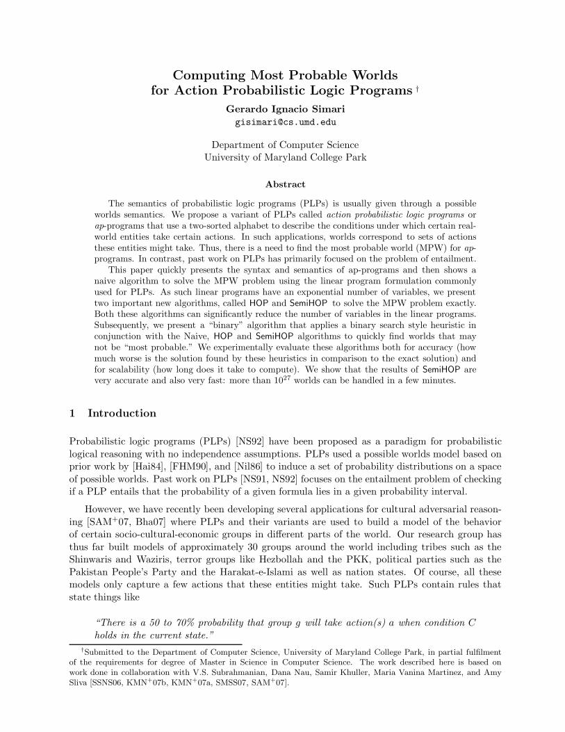
1. kidnap: [0.35, 0.45] ← interOrganizationConflicts.2. kidnap: [0.60, 0.68] ← unDemocratic ∧ internalConflicts.3. armed attacks: [0.42, 0.53] ← typeLeadership(strongSingle) ∧

orgPopularity(moderate).4. armed attacks: [0.93, 1.0] ← statusMilitaryWing(standing).

Figure 1: Four simple rules for modeling the behavior of a group in certain situations.

probabilities for e1, e2, we can only infer an interval for the conjunction and disjunction of e1, e2.(iii) Interval probabilities generalize point probabilities anyway, so our work is also relevant to pointprobabilities.

Definition 2.2 (ap-rules) If F is an action formula, A1, A2, ..., Am are action atoms, B1, . . . , Bn

are non-action atoms, and µ, µ1, ..., µm are ap-annotations, then F : µ← A1 : µ1 ∧ A2 : µ2 ∧ ... ∧Am : µm ∧ B1 ∧ . . . Bm is called an ap-rule. If this rule is named c, then Head(c) denotes F : µ,Bodyact(c) denotes A1 : µ1 ∧ A2 : µ2 ∧ ... ∧ Am : µm, and Bodystate(c) denotes B1 ∧ . . . Bn.

Intuitively, the above ap-rule says that an unnamed entity (e.g. a group g, a person p etc.) willtake action F with probability in the range µ if B1, . . . , Bn are true in the current state (we willdefine this term shortly) and if the unnamed entity will take each action Ai with a probability inthe interval µi for 1 ≤ i ≤ n.

Definition 2.3 (ap-program) An action probabilistic logic program (ap-program for short) is afinite set of ap-rules.

Figure 1 shows a small rule base consisting of some rules we have derived automatically aboutHezbollah using behavioral data from [WAJ+07]. The behavioral data in [WAJ+07] has trackedover 200 terrorist groups for about 20 years from 1980 to 2004. For each year, values have beengathered for about 150 measurable variables for each group in the sample. These variables includeconditions such as tendency to commit assassinations and armed attacks, as well as backgroundinformation about the type of leadership, whether the group is involved in cross border violence, etc.Our automatic derivation of these rules was based on a data mining algorithm we have developed,but is not covered in this work. We show four rules we have extracted for the group Hezbollahin Figure 1. For example, the third rule says that when Hezbollah has a strong, single leader andits popularity is moderate, its propensity to conduct armed attacks has been 42 to 53%. However,when it has had a standing military, its propensity to conduct armed attacks is 93 to 100%.

Definition 2.4 (world/state) A world is any set of ground action atoms. A state is any finiteset of ground non-action atoms.

Example 2.1 Consider the ap-program from Figure 1; there are two ground action atoms: kidnapand armed attacks, and there are therefore a total of 22 = 4 possible worlds. These are: w0 = ∅,w1 = {kidnap}, w2 = {armed attacks}, and w3 = {kidnap, armed attacks}. The following aretwo possible states:

s1 = {statusMilitaryWing(standing), unDemocratic, internalConflicts},s2 = {interOrganizationConflicts , orgPopularity(moderate)}


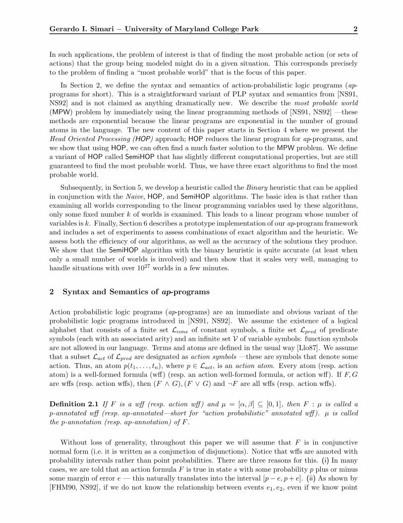
1. d: [0.52, 0.82] ← .2. b ∧ a: [0.55, 0.69] ← d: [0.48, 0.89].

Figure 2: A simple example of an ap-program with action atoms in the body of the rules, which isalready reduced with respect to a certain state.

Note that both worlds and states are just ordinary Herbrand interpretations. As such, it isclear what it means for a state to satisfy Bodystate.

Definition 2.5 Let Π be an ap-program and s a state. The reduction of Π w.r.t. s, denoted by Πs

is {F : µ ← Bodyact | s satisfies Bodystate and F : µ ← Bodyact ∧ Bodystate is a ground instanceof a rule in Π}.

Note that Πs never has any non-action atoms in it. The following is an example of a reductionwith respect to a state.

Example 2.2 Let Π be the ap-program from Figure 1, and suppose we have the following state:

s = {statusMilitaryWing(standing), unDemocratic, internalConflicts}

The reduction of Π with respect to state s is:

Πs = {kidnap : [0.60, 0.68], armed attacks : [0.93, 1.0]}.

Key differences. The key differences between ap-programs and the PLPs of [NS91, NS92] arethat (i) ap-programs have a bipartite structure (action atoms and state atoms) and (ii) they allowarbitrary formulas (including ones with negation) in rule heads ([NS91, NS92] do not). They caneasily be extended to include variable annotations and annotation terms as in [NS91]. Likewise, asin [NS91], they can be easily extended to allow complex formulas rather than just atoms in rulebodies. Due to space restrictions, we do not do either of these in this paper. However, the mostimportant difference between our paper and [NS91, NS92] is that this paper focuses on finding mostprobable worlds, while those papers focus on entailment, which is a fundamentally different problem.

Throughout this paper, we will assume that there is a fixed state s. Hence, once we are givenΠ and s, Πs is fixed. We can associate a fixpoint operator TΠs with Π, s which maps sets of groundap-annotated wffs to sets of ground ap-annotated wffs as follows. We first define an intermediateoperator UΠs(X).

Definition 2.6 Suppose X is a set of ground ap-wffs. We define UΠs(X) = {F : µ | F : µ ←A1 : µ1 ∧ · · · ∧ Am : µm is a ground instance of a rule in Πs and for all 1 ≤ j ≤ m, there is anAj : ηj ∈ X such that ηj ⊆ µj}.

Intuitively, UΠs(X) contains the heads of all rules in Πs whose bodies are deemed to be “true”if the ap-wffs in X are true. However, UΠs(X) may not contain all ground action atoms. Thiscould be because such atoms don’t occur in the head of a rule —UΠs(X) never contains any actionwff that is not in a rule head. The following is an example of the calculation of UΠs(X).


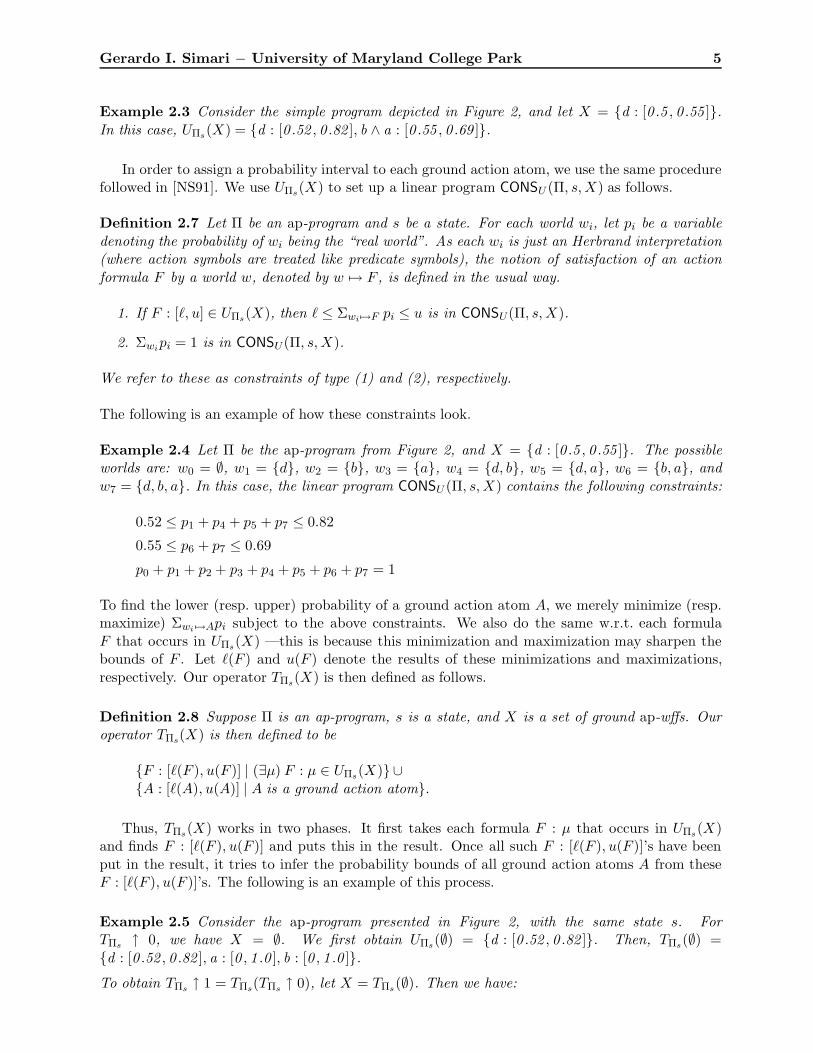
Example 2.3 Consider the simple program depicted in Figure 2, and let X = {d : [0 .5 , 0 .55 ]}.In this case, UΠs(X) = {d : [0 .52 , 0 .82 ], b ∧ a : [0 .55 , 0 .69 ]}.

In order to assign a probability interval to each ground action atom, we use the same procedurefollowed in [NS91]. We use UΠs(X) to set up a linear program CONSU (Π, s, X) as follows.

Definition 2.7 Let Π be an ap-program and s be a state. For each world wi, let pi be a variabledenoting the probability of wi being the “real world”. As each wi is just an Herbrand interpretation(where action symbols are treated like predicate symbols), the notion of satisfaction of an actionformula F by a world w, denoted by w 7→ F , is defined in the usual way.

1. If F : [`, u] ∈ UΠs(X), then ` ≤ Σwi 7→F pi ≤ u is in CONSU(Π, s, X).

2. Σwipi = 1 is in CONSU(Π, s, X).

We refer to these as constraints of type (1) and (2), respectively.

The following is an example of how these constraints look.

Example 2.4 Let Π be the ap-program from Figure 2, and X = {d : [0 .5 , 0 .55 ]}. The possibleworlds are: w0 = ∅, w1 = {d}, w2 = {b}, w3 = {a}, w4 = {d, b}, w5 = {d, a}, w6 = {b, a}, andw7 = {d, b, a}. In this case, the linear program CONSU (Π, s, X) contains the following constraints:

0.52 ≤ p1 + p4 + p5 + p7 ≤ 0.82

0.55 ≤ p6 + p7 ≤ 0.69

p0 + p1 + p2 + p3 + p4 + p5 + p6 + p7 = 1

To find the lower (resp. upper) probability of a ground action atom A, we merely minimize (resp.maximize) Σwi 7→Api subject to the above constraints. We also do the same w.r.t. each formulaF that occurs in UΠs(X) —this is because this minimization and maximization may sharpen thebounds of F . Let `(F ) and u(F ) denote the results of these minimizations and maximizations,respectively. Our operator TΠs(X) is then defined as follows.

Definition 2.8 Suppose Π is an ap-program, s is a state, and X is a set of ground ap-wffs. Ouroperator TΠs(X) is then defined to be

{F : [`(F ), u(F )] | (∃µ) F : µ ∈ UΠs(X)} ∪{A : [`(A), u(A)] | A is a ground action atom}.

Thus, TΠs(X) works in two phases. It first takes each formula F : µ that occurs in UΠs(X)and finds F : [`(F ), u(F )] and puts this in the result. Once all such F : [`(F ), u(F )]’s have beenput in the result, it tries to infer the probability bounds of all ground action atoms A from theseF : [`(F ), u(F )]’s. The following is an example of this process.

Example 2.5 Consider the ap-program presented in Figure 2, with the same state s. ForTΠs ↑ 0, we have X = ∅. We first obtain UΠs(∅) = {d : [0 .52 , 0 .82 ]}. Then, TΠs(∅) ={d : [0 .52 , 0 .82 ], a : [0 , 1 .0 ], b : [0 , 1 .0 ]}.

To obtain TΠs ↑ 1 = TΠs(TΠs ↑ 0), let X = TΠs(∅). Then we have:


UΠs(X) = {d : [0 .52 , 0 .82 ], b ∧ a : [0 .55 , 0 .69 ]}, andTΠs(X) = {d : [0 .52 , 0 .82 ], b ∧ a : [0 .55 , 0 .69 ]}

∪ {A : [`(A), u(A)] | A is a ground action atom }.

In order to infer the probability bounds for all ground action atoms, we need to build a linearprogram using the formulas from UΠs(X) and solve it for each ground atom by minimizing andmaximizing the objective function of the probabilities of the worlds that satisfy each atom. Thepossible worlds are: w0 = ∅, w1 = {d}, w2 = {b}, w3 = {a}, w4 = {d, b}, w5 = {d, a}, w6 = {b, a},and w7 = {d, b, a}. The linear program then consists of the following constraints:

0.52 ≤ p1 + p4 + p5 + p7 ≤ 0.82

0.55 ≤ p6 + p7 ≤ 0.69

p0 + p1 + p2 + p3 + p4 + p5 + p6 + p7 = 1

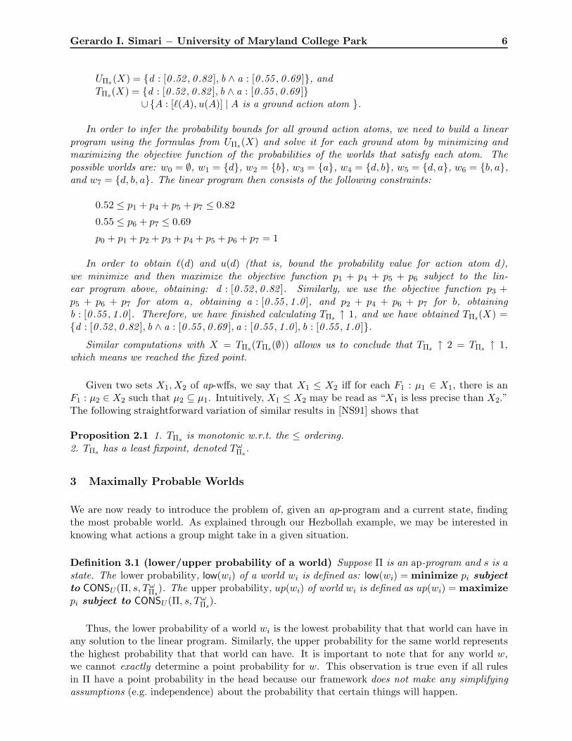
In order to obtain `(d) and u(d) (that is, bound the probability value for action atom d),we minimize and then maximize the objective function p1 + p4 + p5 + p6 subject to the lin-ear program above, obtaining: d : [0 .52 , 0 .82 ]. Similarly, we use the objective function p3 +p5 + p6 + p7 for atom a, obtaining a : [0 .55 , 1 .0 ], and p2 + p4 + p6 + p7 for b, obtainingb : [0 .55 , 1 .0 ]. Therefore, we have finished calculating TΠs ↑ 1, and we have obtained TΠs(X) ={d : [0 .52 , 0 .82 ], b ∧ a : [0 .55 , 0 .69 ], a : [0 .55 , 1 .0 ], b : [0 .55 , 1 .0 ]}.

Similar computations with X = TΠs(TΠs(∅)) allows us to conclude that TΠs ↑ 2 = TΠs ↑ 1,which means we reached the fixed point.

Given two sets X1, X2 of ap-wffs, we say that X1 ≤ X2 iff for each F1 : µ1 ∈ X1, there is anF1 : µ2 ∈ X2 such that µ2 ⊆ µ1. Intuitively, X1 ≤ X2 may be read as “X1 is less precise than X2.”The following straightforward variation of similar results in [NS91] shows that

Proposition 2.1 1. TΠs is monotonic w.r.t. the ≤ ordering.2. TΠs has a least fixpoint, denoted Tω

Πs.

3 Maximally Probable Worlds

We are now ready to introduce the problem of, given an ap-program and a current state, findingthe most probable world. As explained through our Hezbollah example, we may be interested inknowing what actions a group might take in a given situation.

Definition 3.1 (lower/upper probability of a world) Suppose Π is an ap-program and s is astate. The lower probability, low(wi) of a world wi is defined as: low(wi) = minimize pi subjectto CONSU(Π, s, Tω

Πs). The upper probability, up(wi) of world wi is defined as up(wi) = maximize

pi subject to CONSU (Π, s, TωΠs

).

Thus, the lower probability of a world wi is the lowest probability that that world can have inany solution to the linear program. Similarly, the upper probability for the same world representsthe highest probability that that world can have. It is important to note that for any world w,we cannot exactly determine a point probability for w. This observation is true even if all rulesin Π have a point probability in the head because our framework does not make any simplifyingassumptions (e.g. independence) about the probability that certain things will happen.


We now state two simple results that state that checking if the low (resp. up) probabilityof a world exceeds a given bound (called the BOUNDED-LOW and BOUNDED-UP problemsrespectively) is intractable. The hardness results, in both cases, are by reduction from the problemof checking consistency of a generalized probabilistic logic program (PLP-CONS). The problem isin the class EXPTIME.

Proposition 3.1 (BOUNDED-LOW complexity) Given a ground ap-program Π, a state s, aworld w, and a probability threshold pth, deciding if low(w) ≥ pth is NP -hard.

Proof 3.1 We will reduce the PLP-CONS problem to the problem of deciding if a certain world wis such that low(w) ≥ pth for a certain probability value pth. Because PLP-CONS was proven to beNP -hard [FHM90], this reduction will prove that BOUNDED-LOW is NP -hard as well.

Given an instance of PLP-CONS consisting of a program Π and a state s, we build an instanceof BOUNDED-LOW, consisting of an ap-program Π′, a state s′, a world w, and a probabilitythreshold pth in the following manner: program Π′ is equal to Π and state s′ is equal to s, world w

is an arbitrary world, and pth = 0. We must now show that this transformation yields a reductionby proving that Π is consistent in state s if and only if low(w) ≥ 0 with respect to Π′ and state s′:

• Π is consistent ⇒ low(w) ≥ 0 with respect to Π′ in state s′: If Π is consistent, this meansthat CONSU(Π, s, Tω

Πs) is solvable. Therefore, it is clear that any possible world will receive a

probability value greater than or equal to zero.

• low(w) ≥ 0 with respect to Π′ in state s′ ⇒ Π is consistent: If low(w) ≥ 0 with respect to Π instate s′, this means that w has received a probability value greater than or equal to zero, subjectto CONSU (Π, s, Tω

Πs). This is only possible if CONSU(Π, s, Tω

Πs) is solvable, which means that

Π is consistent (this well known property was proved in [NS92]).

To complete the proof, we note that the transformation from a PLP-CONS instance to a BOUNDED-LOW instance can be done in polynomial time with respect to the size of the ap-program given forPLP-CONS.

Proposition 3.2 (BOUNDED-UP complexity) Given a ground ap-program Π, a state s, aworld w, and a probability threshold pth, deciding if up(w) ≤ pth is NP -hard.

Proof 3.2 Analogous to that of Proposition 3.1.

An open problem is to characterize the precise complexity of the BOUNDED-LOW andBOUNDED-UP problems.

The MPW Problem. The most probable world problem (MPW for short) is the problem where,given an ap-program Π and a state s as input, we are required to find a world wi where low(wi) ismaximal. 1

1A similar MPW-Up Problem can also be defined. The most probable world-up problem (MPW-Up) is: givenan ap-program Π and a state s as input, find a world wi where up(wi) is maximal. Due to space constraints, we onlyaddress the MPW problem.


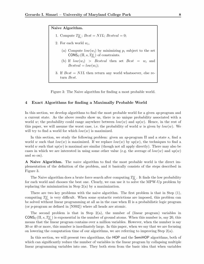
Naive Algorithm.

1. Compute TωΠs

; Best = NIL; Bestval = 0;

2. For each world wi,

(a) Compute low(wi) by minimizing pi subject to the setCONSU (Π, s, Tω

Πs) of constraints.

(b) If low(wi) > Bestval then set Best = wi andBestval = low(wi);

3. If Best = NIL then return any world whatsoever, else re-turn Best.

Figure 3: The Naive algorithm for finding a most probable world.

4 Exact Algorithms for finding a Maximally Probable World

In this section, we develop algorithms to find the most probable world for a given ap-program anda current state. As the above results show us, there is no unique probability associated with aworld w; the probability could range anywhere between low(w) and up(w). Hence, in the rest ofthis paper, we will assume the worst case, i.e. the probability of world w is given by low(w). Wewill try to find a world for which low(w) is maximized.

In this section, we study the following problem: given an ap-program Π and a state s, find aworld w such that low(w) is maximized. If we replace low(w) by up(w), the techniques to find aworld w such that up(w) is maximal are similar (though not all apply directly). There may also becases in which we are interested in using some other value (e.g. the average of low(w) and up(w)and so on).

A Naive Algorithm. The naive algorithm to find the most probable world is the direct im-plementation of the definition of the problem, and it basically consists of the steps described inFigure 3.

The Naive algorithm does a brute force search after computing TωΠs

. It finds the low probabilityfor each world and chooses the best one. Clearly, we can use it to solve the MPW-Up problem byreplacing the minimization in Step 2(a) by a maximization.

There are two key problems with the naive algorithm. The first problem is that in Step (1),computing Tω

Πsis very difficult. When some syntactic restrictions are imposed, this problem can

be solved without linear programming at all as in the case when Π is a probabilistic logic program(or p-program as defined in [NS92]) where all heads are atomic.

The second problem is that in Step 2(a), the number of (linear program) variables inCONSU(Π, s, Tω

Πs) is exponential in the number of ground atoms. When this number is, say 20, this

means that the linear program contains over a million variables. However, when the number is say30 or 40 or more, this number is inordinately large. In this paper, when we say that we are focusingon lowering the computation time of our algorithms, we are referring to improving Step 2(a).

In this section, we will present two algorithms, the HOP and the SemiHOP algorithms, both ofwhich can significantly reduce the number of variables in the linear program by collapsing multiplelinear programming variables into one. They both stem from the basic idea that when variables


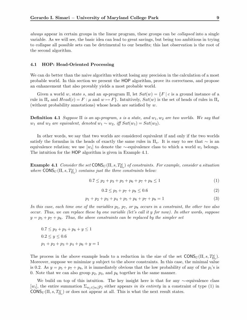
always appear in certain groups in the linear program, these groups can be collapsed into a singlevariable. As we will see, the basic idea can lead to great savings, but being too ambitious in tryingto collapse all possible sets can be detrimental to our benefits; this last observation is the root ofthe second algorithm.

4.1 HOP: Head-Oriented Processing

We can do better than the naive algorithm without losing any precision in the calculation of a mostprobable world. In this section we present the HOP algorithm, prove its correctness, and proposean enhancement that also provably yields a most probable world.

Given a world w, state s, and an ap-program Π, let Sat(w) = {F | c is a ground instance of arule in Πs and Head(c) = F : µ and w 7→ F}. Intuitively, Sat(w) is the set of heads of rules in Πs

(without probability annotations) whose heads are satisfied by w.

Definition 4.1 Suppose Π is an ap-program, s is a state, and w1, w2 are two worlds. We say thatw1 and w2 are equivalent, denoted w1 ∼ w2, iff Sat(w1) = Sat(w2).

In other words, we say that two worlds are considered equivalent if and only if the two worldssatisfy the formulas in the heads of exactly the same rules in Πs. It is easy to see that ∼ is anequivalence relation; we use [wi] to denote the ∼-equivalence class to which a world wi belongs.The intuition for the HOP algorithm is given in Example 4.1.

Example 4.1 Consider the set CONSU (Π, s, TωΠs

) of constraints. For example, consider a situationwhere CONSU (Π, s, Tω

Πs) contains just the three constraints below:

0.7 ≤ p2 + p3 + p5 + p6 + p7 + p8 ≤ 1 (1)

0.2 ≤ p5 + p7 + p8 ≤ 0.6 (2)

p1 + p2 + p3 + p4 + p5 + p6 + p7 + p8 = 1 (3)

In this case, each time one of the variables p5, p7, or p8 occurs in a constraint, the other two alsooccur. Thus, we can replace these by one variable (let’s call it y for now). In other words, supposey = p5 + p7 + p8. Thus, the above constraints can be replaced by the simpler set

0.7 ≤ p2 + p3 + p6 + y ≤ 1

0.2 ≤ y ≤ 0.6

p1 + p2 + p3 + p4 + p6 + y = 1

The process in the above example leads to a reduction in the size of the set CONSU(Π, s, TωΠs

).Moreover, suppose we minimize y subject to the above constraints. In this case, the minimal valueis 0.2. As y = p5 + p7 + p8, it is immediately obvious that the low probability of any of the pi’s is0. Note that we can also group p2, p3, and p6 together in the same manner.

We build on top of this intuition. The key insight here is that for any ∼-equivalence class[wi], the entire summation Σwj∈[wi]pj either appears in its entirety in a constraint of type (1) inCONSU(Π, s, Tω

Πs) or does not appear at all. This is what the next result states.


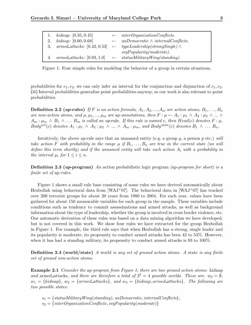
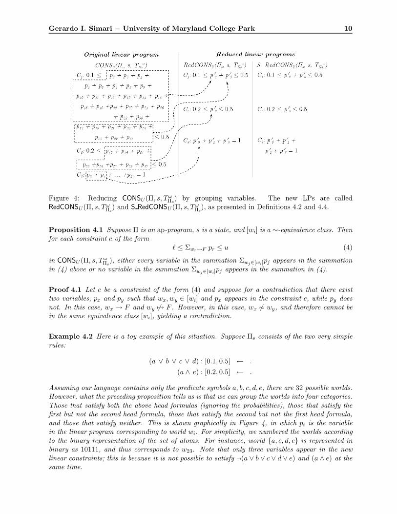
Figure 4: Reducing CONSU(Π, s, TωΠs

) by grouping variables. The new LPs are calledRedCONSU(Π, s, Tω

Πs) and S RedCONSU (Π, s, Tω

Πs), as presented in Definitions 4.2 and 4.4.

Proposition 4.1 Suppose Π is an ap-program, s is a state, and [wi] is a ∼-equivalence class. Thenfor each constraint c of the form

` ≤ Σwr 7→F pr ≤ u (4)

in CONSU (Π, s, TωΠs

), either every variable in the summation Σwj∈[wi]pj appears in the summationin (4) above or no variable in the summation Σwj∈[wi]pj appears in the summation in (4).

Proof 4.1 Let c be a constraint of the form (4) and suppose for a contradiction that there existtwo variables, px and py such that wx, wy ∈ [wi] and px appears in the constraint c, while py doesnot. In this case, wx 7→ F and wy 67→ F . However, in this case, wx 6∼ wy, and therefore cannot bein the same equivalence class [wi], yielding a contradiction.

Example 4.2 Here is a toy example of this situation. Suppose Πs consists of the two very simplerules:

(a ∨ b ∨ c ∨ d) : [0.1, 0.5] ← .

(a ∧ e) : [0.2, 0.5] ← .

Assuming our language contains only the predicate symbols a, b, c, d, e, there are 32 possible worlds.However, what the preceding proposition tells us is that we can group the worlds into four categories.Those that satisfy both the above head formulas (ignoring the probabilities), those that satisfy thefirst but not the second head formula, those that satisfy the second but not the first head formula,and those that satisfy neither. This is shown graphically in Figure 4, in which pi is the variablein the linear program corresponding to world wi. For simplicity, we numbered the worlds accordingto the binary representation of the set of atoms. For instance, world {a, c, d, e} is represented inbinary as 10111, and thus corresponds to w23. Note that only three variables appear in the newlinear constraints; this is because it is not possible to satisfy ¬(a ∨ b ∨ c ∨ d ∨ e) and (a ∧ e) at thesame time.


Effectively, what we have done is to modify the number of variables in the linear program from2card(Lact) to 2card(Πs) —a saving that can be significant in some cases (though not always, and insome cases it can actually result in an increase in size). The number of constraints in the linearprogram stays the same. Formally speaking, we define a reduced set of constraints as follows.

Definition 4.2 (RedCONSU (Π, s, TωΠs

)) For each equivalence class [wi],RedCONSU(Π, s, Tω

Πs) uses a variable p′i to denote the summation of the probability of each

of the worlds in [wi]. For each ap-wff F : [`, u] in TωΠs

, RedCONSU(Π, s, TωΠs

) contains theconstraint:

` ≤ Σ[wi] 7→F p′i ≤ u.

Here, [wi] 7→ F means that some world in [wi] satisfies F . In addition, RedCONSU (Π, s, TωΠs

)contains the constraint

Σ[wi]p′i = 1.

When reasoning about RedCONSU(Π, s, TωΠs

), we can do even better than mentioned above. Theresult below states that to find the most probable world, we only need to look at the equivalenceclasses that are of cardinality 1.

Theorem 4.1 Suppose Π is an ap-program, s is a state, and wi is a world. If card([wi]) > 1, thenlow(wi) = 0.

Proof 4.2 Immediate, by observing that there are no restrictions on the values assigned to thevariables that correspond to worlds in the same ∼-class. If there is more than one world in aclass [wx], there is always a solution that assigns zero to each variable pi such that wi ∈ [wx], andtherefore low(wi) = 0.

Going back to Example 4.1, we can conclude that low(w5) = low(w7) = low(w8) = 0. As aconsequence of this result, we can suggest the Head Oriented Processing (HOP) algorithm whichworks as follows. First we present some simple notation. Let FixedWff (Π, s) = {F | F : µ ∈UΠs(Tω

Πs)}. Given a set X ⊆ FixedWff (Π, s), we define Formula(X, Π, s) to be

∧

G∈X

G ∧∧

G′∈FixedWff (Π,s)−X

¬G′.

Here, Formula(X, Π, s) is the formula which says that X consists of all and only those formulasin FixedWff (Π, s) that are true. Given two sets X1, X2 ⊆ FixedWff (Π, s), we say that X1 ∼ X2 ifand only if Formula(X1, Π, s) and Formula(X2, Π, s) are logically equivalent.

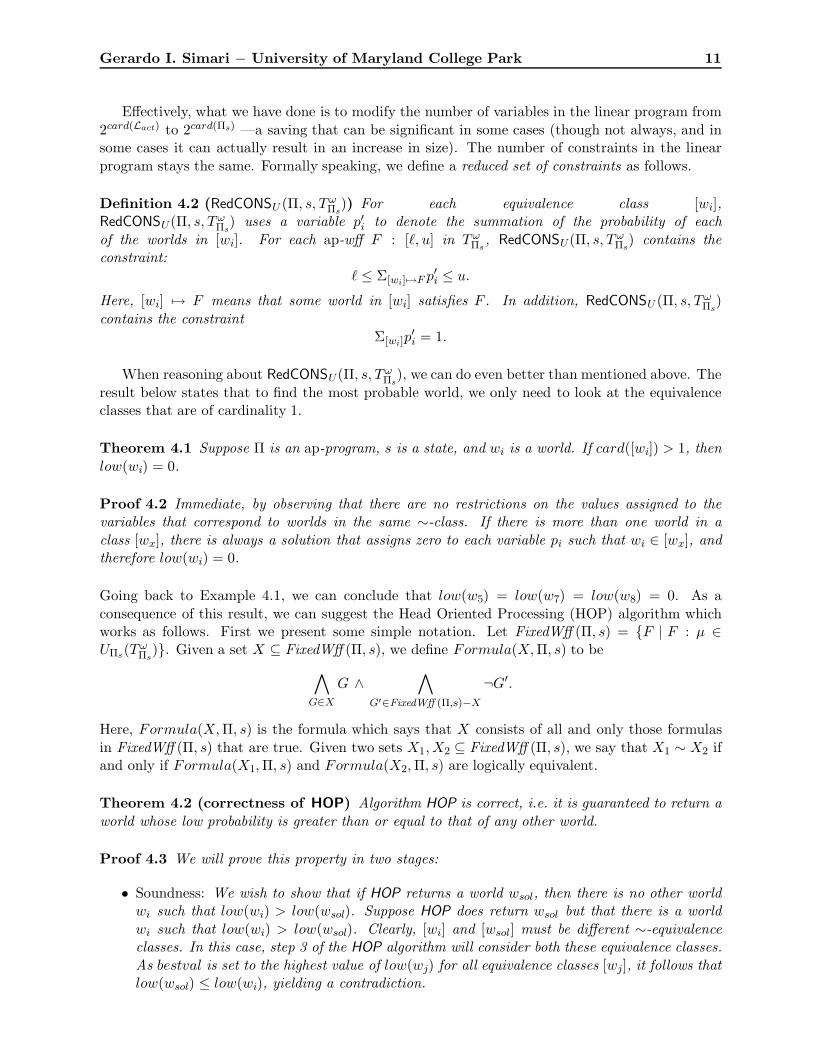
Theorem 4.2 (correctness of HOP) Algorithm HOP is correct, i.e. it is guaranteed to return aworld whose low probability is greater than or equal to that of any other world.

Proof 4.3 We will prove this property in two stages:

• Soundness: We wish to show that if HOP returns a world wsol, then there is no other worldwi such that low(wi) > low(wsol). Suppose HOP does return wsol but that there is a worldwi such that low(wi) > low(wsol). Clearly, [wi] and [wsol] must be different ∼-equivalenceclasses. In this case, step 3 of the HOP algorithm will consider both these equivalence classes.As bestval is set to the highest value of low(wj) for all equivalence classes [wj], it follows thatlow(wsol) ≤ low(wi), yielding a contradiction.


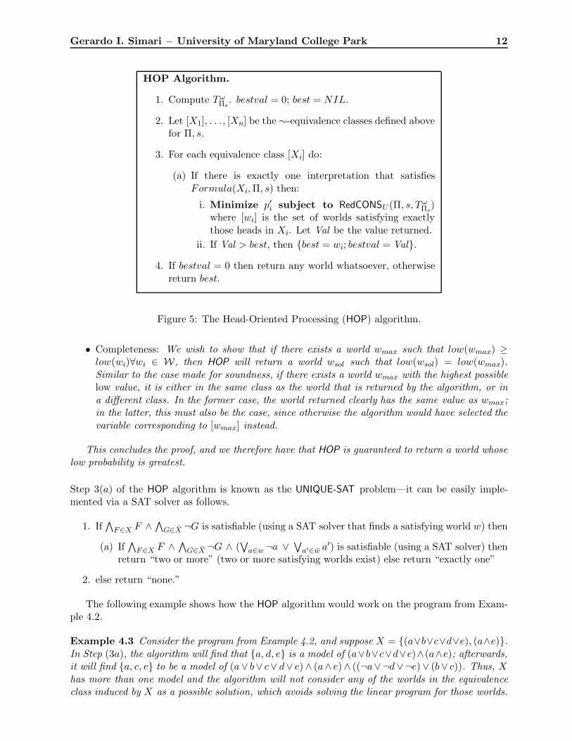
HOP Algorithm.

1. Compute TωΠs

. bestval = 0; best = NIL.

2. Let [X1], . . . , [Xn] be the ∼-equivalence classes defined abovefor Π, s.

3. For each equivalence class [Xi] do:

(a) If there is exactly one interpretation that satisfiesFormula(Xi, Π, s) then:

i. Minimize p′i subject to RedCONSU (Π, s, TωΠs

)where [wi] is the set of worlds satisfying exactlythose heads in Xi. Let Val be the value returned.

ii. If Val > best, then {best = wi; bestval = Val}.

4. If bestval = 0 then return any world whatsoever, otherwisereturn best.

Figure 5: The Head-Oriented Processing (HOP) algorithm.

• Completeness: We wish to show that if there exists a world wmax such that low(wmax) ≥low(wi)∀wi ∈ W, then HOP will return a world wsol such that low(wsol) = low(wmax).Similar to the case made for soundness, if there exists a world wmax with the highest possiblelow value, it is either in the same class as the world that is returned by the algorithm, or ina different class. In the former case, the world returned clearly has the same value as wmax;in the latter, this must also be the case, since otherwise the algorithm would have selected thevariable corresponding to [wmax] instead.

This concludes the proof, and we therefore have that HOP is guaranteed to return a world whoselow probability is greatest.

Step 3(a) of the HOP algorithm is known as the UNIQUE-SAT problem—it can be easily imple-mented via a SAT solver as follows.

1. If∧

F∈X F ∧∧

G∈X̄ ¬G is satisfiable (using a SAT solver that finds a satisfying world w) then

(a) If∧

F∈X F ∧∧

G∈X̄ ¬G ∧ (∨

a∈w ¬a ∨∨

a′∈w̄ a′) is satisfiable (using a SAT solver) thenreturn “two or more” (two or more satisfying worlds exist) else return “exactly one”

2. else return “none.”

The following example shows how the HOP algorithm would work on the program from Exam-ple 4.2.

Example 4.3 Consider the program from Example 4.2, and suppose X = {(a∨b∨c∨d∨e), (a∧e)}.In Step (3a), the algorithm will find that {a, d, e} is a model of (a∨b∨c∨d∨e)∧(a∧e); afterwards,it will find {a, c, e} to be a model of (a∨ b∨ c∨ d∨ e)∧ (a∧ e)∧ ((¬a∨¬d∨¬e)∨ (b∨ c)). Thus, X

has more than one model and the algorithm will not consider any of the worlds in the equivalenceclass induced by X as a possible solution, which avoids solving the linear program for those worlds.


The worst-case complexity of HOP is, as its Naive counterpart, exponential. However, HOPcan sometimes (but not always) be preferable to the Naive algorithm. The number of vari-ables in RedCONSU(Π, s, Tω

Πs) is 2card(Πs), which is much smaller than the number of variables

in CONSU (Π, s, TωΠs

) when the number of ground rules whose bodies are satisfied by state s issmaller than the number of ground atoms. The checks required to find all the equivalence classes[Xi] take time proportional to 22∗card(Πs). Lastly, HOP avoids solving the reduced linear programfor all the non-singleton equivalence classes (for instance, in Example 4.3, the algorithm avoidssolving the LP three times). This last saving, however, comes at the price of solving SAT twice foreach equivalence class and the time required to find the [Xi]’s. We will now explore a way in whichwe can trade off computation time against how many of these savings we obtain, again withoutgiving up obtaining an exact solution.

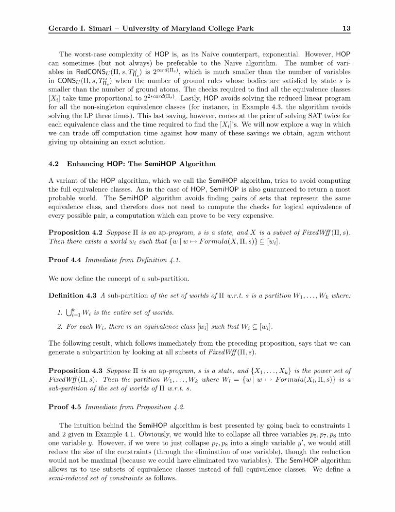
4.2 Enhancing HOP: The SemiHOP Algorithm

A variant of the HOP algorithm, which we call the SemiHOP algorithm, tries to avoid computingthe full equivalence classes. As in the case of HOP, SemiHOP is also guaranteed to return a mostprobable world. The SemiHOP algorithm avoids finding pairs of sets that represent the sameequivalence class, and therefore does not need to compute the checks for logical equivalence ofevery possible pair, a computation which can prove to be very expensive.

Proposition 4.2 Suppose Π is an ap-program, s is a state, and X is a subset of FixedWff (Π, s).Then there exists a world wi such that {w | w 7→ Formula(X, Π, s)} ⊆ [wi].

Proof 4.4 Immediate from Definition 4.1.

We now define the concept of a sub-partition.

Definition 4.3 A sub-partition of the set of worlds of Π w.r.t. s is a partition W1, . . . , Wk where:

1.⋃k

i=1 Wi is the entire set of worlds.

2. For each Wi, there is an equivalence class [wi] such that Wi ⊆ [wi].

The following result, which follows immediately from the preceding proposition, says that we cangenerate a subpartition by looking at all subsets of FixedWff (Π, s).

Proposition 4.3 Suppose Π is an ap-program, s is a state, and {X1, . . . , Xk} is the power set ofFixedWff (Π, s). Then the partition W1, . . . , Wk where Wi = {w | w 7→ Formula(Xi, Π, s)} is asub-partition of the set of worlds of Π w.r.t. s.

Proof 4.5 Immediate from Proposition 4.2.

The intuition behind the SemiHOP algorithm is best presented by going back to constraints 1and 2 given in Example 4.1. Obviously, we would like to collapse all three variables p5, p7, p8 intoone variable y. However, if we were to just collapse p7, p8 into a single variable y′, we would stillreduce the size of the constraints (through the elimination of one variable), though the reductionwould not be maximal (because we could have eliminated two variables). The SemiHOP algorithmallows us to use subsets of equivalence classes instead of full equivalence classes. We define asemi-reduced set of constraints as follows.


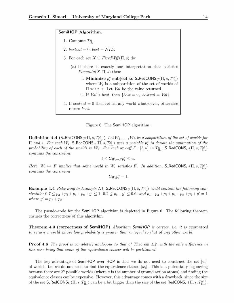
SemiHOP Algorithm.

1. Compute TωΠs

.

2. bestval = 0; best = NIL.

3. For each set X ⊆ FixedWff (Π, s) do:

(a) If there is exactly one interpretation that satisfiesFormula(X, Π, s) then:

i. Minimize p?i subject to S RedCONSU (Π, s, Tω

Πs)

where Wi is a subpartition of the set of worlds ofΠ w.r.t. s. Let Val be the value returned.

ii. If Val > best, then {best = wi; bestval = Val}.

4. If bestval = 0 then return any world whatsoever, otherwisereturn best.

Figure 6: The SemiHOP algorithm.

Definition 4.4 (S RedCONSU(Π, s, TωΠs

)) Let W1, . . . , Wk be a subpartition of the set of worlds forΠ and s. For each Wi, S RedCONSU(Π, s, Tω

Πs) uses a variable p?

i to denote the summation of theprobability of each of the worlds in Wi. For each ap-wff F : [`, u] in Tω

Πs, S RedCONSU (Π, s, Tω

Πs)

contains the constraint:` ≤ ΣWi 7→F p?

i ≤ u.

Here, Wi 7→ F implies that some world in Wi satisfies F . In addition, S RedCONSU (Π, s, TωΠs

)contains the constraint

ΣWip?i = 1

Example 4.4 Returning to Example 4.1, S RedCONSU(Π, s, TωΠs

) could contain the following con-straints: 0.7 ≤ p2 +p3 +p5 +p6 +y′ ≤ 1, 0.2 ≤ p5 +y′ ≤ 0.6, and p1 +p2 +p3 +p4 +p5 +p6 +y′ = 1where y′ = p7 + p8.

The pseudo-code for the SemiHOP algorithm is depicted in Figure 6. The following theoremensures the correctness of this algorithm.

Theorem 4.3 (correctness of SemiHOP) Algorithm SemiHOP is correct, i.e. it is guaranteedto return a world whose low probability is greater than or equal to that of any other world.

Proof 4.6 The proof is completely analogous to that of Theorem 4.2, with the only difference inthis case being that some of the equivalence classes will be partitioned.

The key advantage of SemiHOP over HOP is that we do not need to construct the set [wi]of worlds, i.e. we do not need to find the equivalence classes [wi]. This is a potentially big savingbecause there are 2n possible worlds (where n is the number of ground action atoms) and finding theequivalence classes can be expensive. However, this advantage comes with a drawback, since the sizeof the set S RedCONSU(Π, s, Tω

Πs) can be a bit bigger than the size of the set RedCONSU(Π, s, Tω

Πs).


5 The Binary Heuristic

In this section, we introduce a heuristic called the Binary Heuristic that can be utilized in conjunc-tion with any of the three exact algorithms described thus far (Naive, HOP, and SemiHOP) in thepaper. The basic idea behind the Binary Heuristic is to limit the number of variables in the linearprograms associated with the Naive, HOP, and SemiHOP algorithms to a fixed number k that ischosen by the user.

Suppose we use VNaive,VHOP, and VSemiHOP to denote the set of variables occurring in the linearprograms CONSU (Π, s, Tω

Πs), RedCONSU(Π, s, Tω

Πs) and S RedCONSU(Π, s, Tω

Πs), respectively. Note

that all these linear programs contain two kinds of constraints:

• Interval constraints which have the form ` ≤ pi1 + · · ·+ pim ≤ u and

• A single equality constraint of the form p1 + · · ·+ pn = 1.

Let VkNaive,Vk

HOP,VkSemiHOP be some subset of k variables from each of these sets, respectively. Let

CONS be one of CONSU (Π, s, TωΠs

), RedCONSU (Π, s, TωΠs

), or S RedCONSU (Π, s, TωΠs

). We nowconstruct a linear program CONS′ from CONS as follows.

• For all constraints of the form` ≤ pi1 + · · ·+ pim ≤ u

remove all variables in the summation that do not occur in the selected set of k variables andre-set the lower bound to 0.

• For the one constraint of the form p1 + · · ·+ pn = 1, remove all variables in the summationthat do not occur in the selected set of k variables and replace the equality “=” by “≤”.

Example 5.1 Consider the program from Example 4.2, and suppose m = 10 and CONS refers tothe constraints associated with the naive algorithm which has 32 worlds altogether. Then, we canselect a sample of ten worlds such as

Wm = {w2, w4, w8, w10, w12, w16, w18, w22, w23, w25}

Now, CONS′(Π, s, TωΠs

) contains the following constraints:

0 ≤ p2 + p4 + p8 + p10 + p12 + p16 + p18 + p22 + p23 + p25 ≤ 0.50 ≤ p23 + p25 ≤ 0.5p2 + p4 + p8 + p10 + p12 + p16 + p18 + p22 + p23 + p25 ≤ 1

Theorem 5.1 Let Π be an ap-program, m > 0 be an integer, and s be a state. Then ev-ery solution of CONS is also a solution of CONS′ where CONS is one of CONSU (Π, s, Tω

Πs),

RedCONSU(Π, s, TωΠs

), or S RedCONSU (Π, s, TωΠs

) and CONS′ is constructed according to the aboveconstruction.


Proof 5.1 (i) Suppose σ is a solution to CONS. For any interval constraint

` ≤ pi1 + · · ·+ pim ≤ u

deleting some terms from the summation preserves the upper bound and clearly the summation stillis greater than or equal to 0. Hence, σ is a solution to the modified interval constraint in CONS′.For the equality constraint p1 + . . . + pn = 1, removing some variables from the summation causesthe resulting sum (under the solution σ) to be less than or equal to 1 and hence the correspondingconstraint in CONS′ is satisfied by σ.

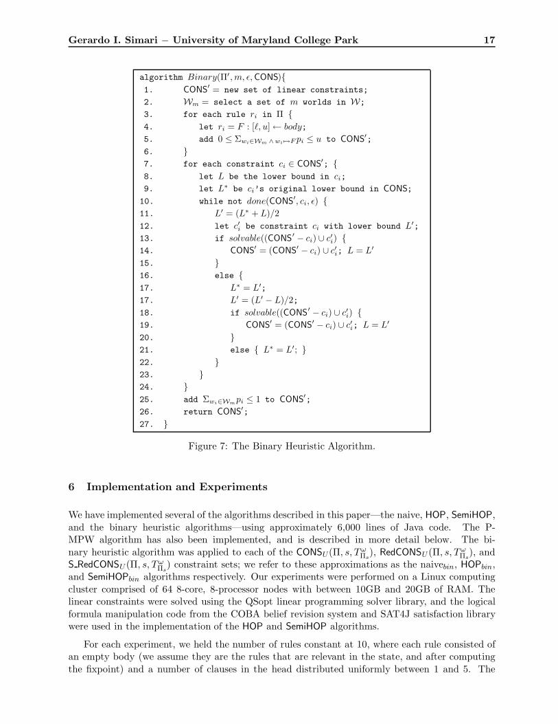
A major problem with the above result is that CONS′ is always satisfiable because setting allvariables to have value 0 is a solution. The binary algorithm tries to tighten the lower bound in theinterval constraints involved so that we have a set of solutions that more closely mirror the originalset. It does this by looking at each interval constraint in CONS′ and trying to set the lower boundof that constraint first to `/2 where ` is the lower bound of the corresponding constraint in CONS.If the resulting set of constraints is satisfiable, it increases it to 3`/4, otherwise it reduces it to `/4.This is repeated for different interval constraints until reasonable tightness is achieved. It should benoted that the order in which the constraints are processed is important - different orders can leadto different CONS′ being generated. The detailed algorithm is shown in Figure 7. The algorithmis called with Π′ = Tω

Πs, and CONS equal to one of CONSU , RedCONS, or S RedCONS.

The Binary algorithm takes a chance. Rather than use a very crude estimate of the lower boundin the constraints (such as 0, the starting point), it tries to “pull” the lower bounds as close tothe original lower bounds as possible in the expectation that the revised linear program is closer inspirit to the original linear program. Here is an example of this process.

Example 5.2 Consider the following very simple program:

a ∧ b : [0.8, 0.9]← .

a ∧ c : [0.2, 0.3]← .

Let W = {w0 = ∅, w1 = {a}, w2 = {b}, w3 = {c}, w4 = {a, b}, w5 = {a, c}, w6 = {b, c}, w7 ={a, b, c}}, but suppose m = 4 and we select a sample of four worlds Wm = {w0, w2, w6, w7}. Now,assuming s = ∅, CONS′(Π, s, Tω

Πs) contains the following constraints:

0 ≤ p7 ≤ 0.90 ≤ p7 ≤ 0.3p0 + p2 + p6 + p7 ≤ 1

which is clearly solvable, but yielding the all-zero solution. The binary heuristic will then modifythe first constraint so that its lower bound is 0.4 and, since this new program is unsolvable, willsubsequently adjust it to 0.2. At this point, the program is now back to being solvable, and onemore iteration leaves the lower bound at (0.4 + 0.2)/2 = 0.3, which results once again in a solvableprogram. At this point, we decide to stop, and the final value of the lower bound is thus 0.3. Thealgorithm then moves on to the following constraint, and adjusts its lower bound first to 0.1 andthen to 0.15, and decides to stop. The final set of constraints is then:

0.3 ≤ p7 ≤ 0.90.15 ≤ p7 ≤ 0.3p0 + p2 + p6 + p7 ≤ 1


algorithm Binary(Π′, m, ε, CONS){1. CONS′ = new set of linear constraints;

2. Wm = select a set of m worlds in W;

3. for each rule ri in Π {4. let ri = F : [`, u]← body;

5. add 0 ≤ Σwi∈Wm ∧wi 7→F pi ≤ u to CONS′;

6. }7. for each constraint ci ∈ CONS′; {8. let L be the lower bound in ci;

9. let L∗ be ci’s original lower bound in CONS;

10. while not done(CONS′, ci, ε) {11. L′ = (L∗ + L)/212. let c′i be constraint ci with lower bound L′;

13. if solvable((CONS′ − ci) ∪ c′i) {14. CONS′ = (CONS′ − ci) ∪ c′i; L = L′

15. }16. else {17. L∗ = L′;

17. L′ = (L′ − L)/2;18. if solvable((CONS′ − ci) ∪ c′i) {19. CONS′ = (CONS′ − ci) ∪ c′i; L = L′

20. }21. else { L∗ = L′; }22. }23. }24. }25. add Σwi∈Wmpi ≤ 1 to CONS′;

26. return CONS′;

27. }

Figure 7: The Binary Heuristic Algorithm.

6 Implementation and Experiments

We have implemented several of the algorithms described in this paper—the naive, HOP, SemiHOP,and the binary heuristic algorithms—using approximately 6,000 lines of Java code. The P-MPW algorithm has also been implemented, and is described in more detail below. The bi-nary heuristic algorithm was applied to each of the CONSU(Π, s, Tω

Πs), RedCONSU (Π, s, Tω

Πs), and

S RedCONSU (Π, s, TωΠs

) constraint sets; we refer to these approximations as the naivebin, HOPbin,and SemiHOPbin algorithms respectively. Our experiments were performed on a Linux computingcluster comprised of 64 8-core, 8-processor nodes with between 10GB and 20GB of RAM. Thelinear constraints were solved using the QSopt linear programming solver library, and the logicalformula manipulation code from the COBA belief revision system and SAT4J satisfaction librarywere used in the implementation of the HOP and SemiHOP algorithms.

For each experiment, we held the number of rules constant at 10, where each rule consisted ofan empty body (we assume they are the rules that are relevant in the state, and after computingthe fixpoint) and a number of clauses in the head distributed uniformly between 1 and 5. The


probability intervals were also generated randomly, making sure that the lower bound was lessthan or equal to the upper bound. All random number selection were implemented using therandom number generator provided by Java. The experiments then consisted of the following: (i)generate a new ap-program and send it to each of the three algorithms, (ii) vary the number ofworlds from 32 to 16,384, performing at least 10 runs for each value and recording the averagetime taken by each algorithm, and (iii) measure the quality of SemiHOP and all algorithms thatuse the binary heuristic by calculating the average distance from the solution found by the exactalgorithm. Due to the immense time complexity of the HOP algorithm, we do not directly compareits performance to the naive algorithm or SemiHOP. In the discussion below we use the metricruledensity = Lact

card(T ωΠs

)to represent the size of the ap-program; this allows for the comparison of

the naive and HOP and SemiHOP algorithms as the number of worlds increases.

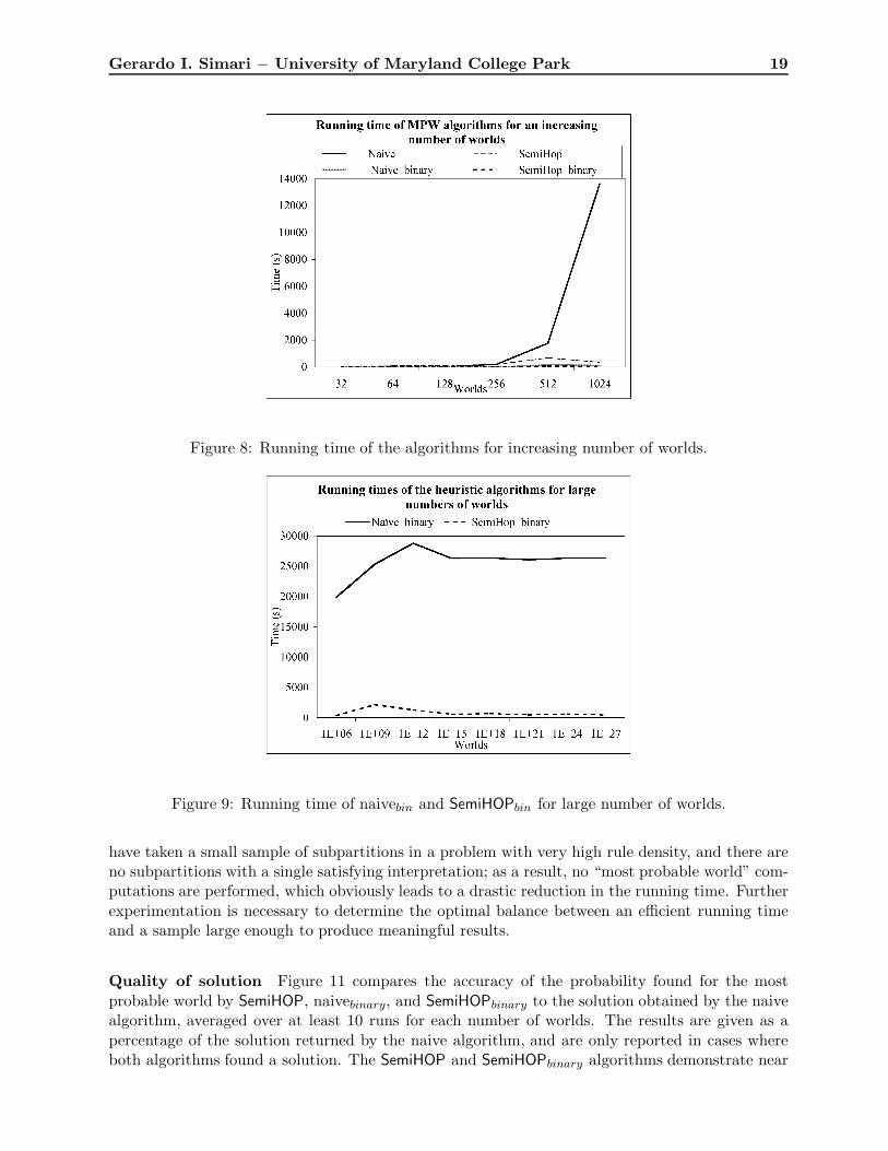
Running time Figure 8 shows the running times for each of the naive, SemiHOP, naivebinary,and SemiHOPbinary algorithms for increasing number of worlds. As expected, the binary searchapproximation algorithm is superior to the exact algorithms in terms of computation time, whenapplied to both the naive and SemiHOP contstraint sets. With a sample size of 25%, naivebinary andSemiHOPbinary take only about 132.6 seconds and 58.19 seconds for instances with 1,024 worlds,whereas the naive algorithm requires almost 4 hours (13,636.23 seconds). This result demonstratesthat the naive algorithm is more or less useless and takes prohibitive amounts of time, even forsmall instances. Similarly, the checks for logical equivalence required to obtain each [wi] for HOPcause the algorithm to consistently require an exorbitant amount of time; for instances with only128 worlds, HOP takes 58,064.74 seconds, which is much greater even than the naive algorithmfor 1024 worlds. Even when using the binary heuristic to further reduce the number of variables,HOPbin still requires a prohibitively large amount of time.

At low rule densities, SemiHOP runs slower than the naive algorithm; with 10 rules, SemiHOPuses 18.75 seconds and 122.44 seconds for 128 worlds, while the naive algorithm only requires1.79 seconds and 19.99 seconds respectively. However, SemiHOP vastly outperforms naive forproblems with higher densities—358.3 seconds versus 13,636.23 seconds for 1,024 worlds—whichmore accurately reflect real-world problems in which the number of possible worlds is far greaterthan the number of ap-rules. Because the SemiHOP algorithm uses subpartions rather than uniqueequivalence classes in the RedCONSU (Π, s, Tω

Πs) constraints, the algorithm overhead is much lower

than that of the HOP algorithm, and thus yields a more efficient running time.

The reduction in the size of the set of constraints afforded by the binary heuristic algorithmallows us to apply the naive and SemiHOP algorithms to much larger ap-programs. In Figure 9, weexamine the running times of the naivebin and SemiHOPbin algorithms for large numbers of worlds(up to 290 or about 1.23794×1027 possible worlds) with a sample size for the binary heuristic of 2%;this is to ensure that the reduced linear program is indeed tractable. SemiHOPbinary consistentlytakes less time than naivebinary, though both algorithms still perform rather well. For 1.23794×1027

possible worlds, naivebinary takes an average 26,325.1 seconds while SemiHOPbinary requires only458.07 seconds. This difference occurs because |S RedCONSU (Π, s, Tω

Πs)| < |CONSU(Π, s, Tω

Πs)|

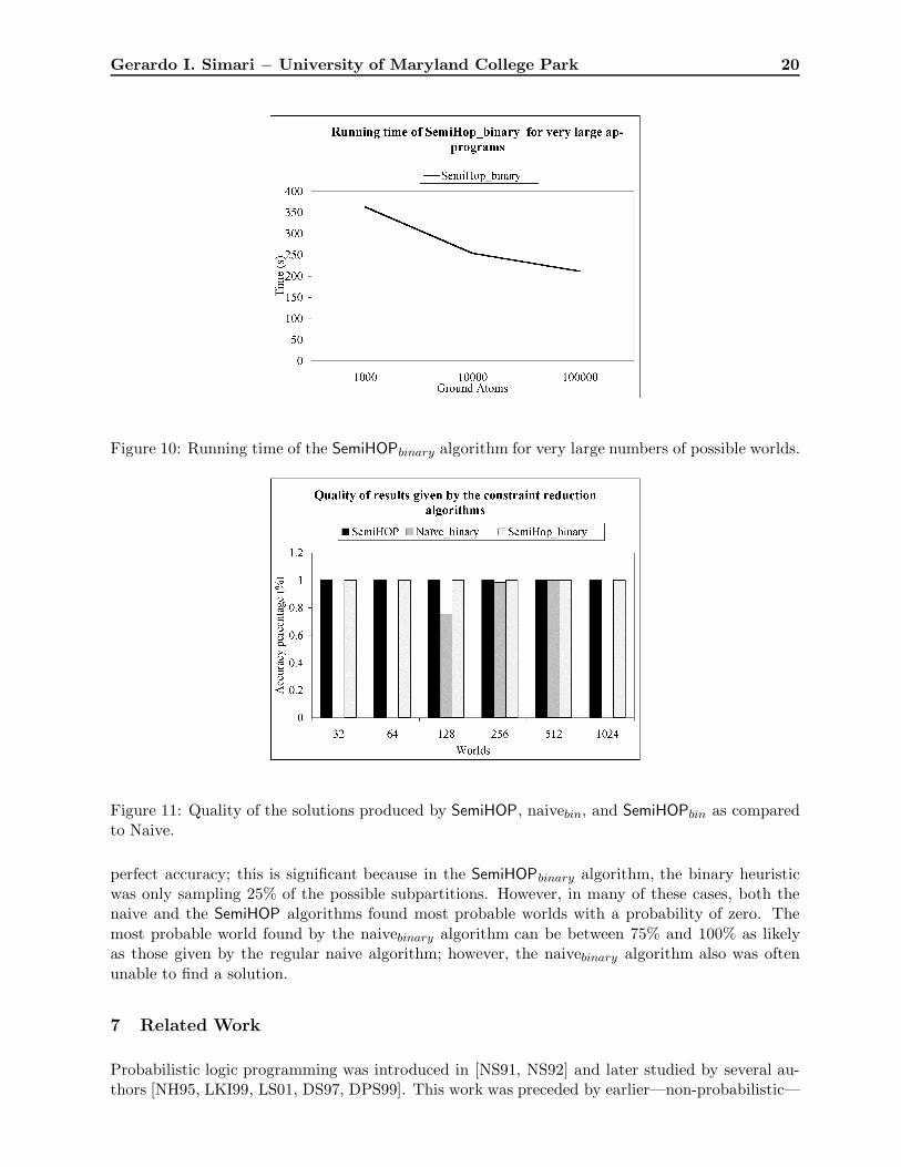
that is the heuristic algorithm is further reducing an already smaller constraint set. In addition,because SemiHOP only solves the linear constraint problem when there is exactly one satisfyinginterpretation for a subpartition, it performs fewer computations overall. Because of this prop-erty, experiments running SemiHOPbinary on problems with very large ap-programs (from 1,000 to100,000 ground atoms) only take around 300 seconds using a 2% sample rate. However, this aspectof the SemiHOP algorithm can also lead to some anomolous behavior, where the running time willappear to decrease as the number of worlds increases. Figure 10 illustrates this anomaly, as thecomputation time appears to decrease with very large numbers of worlds. This occurs when we


Figure 8: Running time of the algorithms for increasing number of worlds.

Figure 9: Running time of naivebin and SemiHOPbin for large number of worlds.

have taken a small sample of subpartitions in a problem with very high rule density, and there areno subpartitions with a single satisfying interpretation; as a result, no “most probable world” com-putations are performed, which obviously leads to a drastic reduction in the running time. Furtherexperimentation is necessary to determine the optimal balance between an efficient running timeand a sample large enough to produce meaningful results.

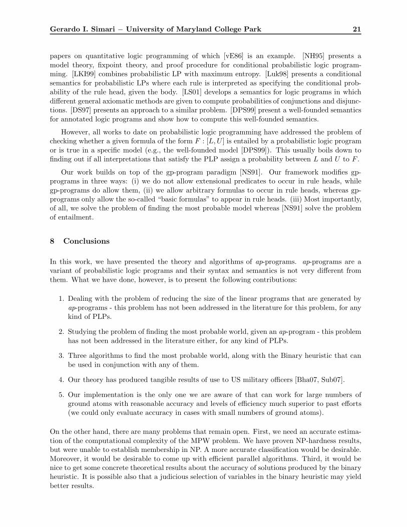
Quality of solution Figure 11 compares the accuracy of the probability found for the mostprobable world by SemiHOP, naivebinary, and SemiHOPbinary to the solution obtained by the naivealgorithm, averaged over at least 10 runs for each number of worlds. The results are given as apercentage of the solution returned by the naive algorithm, and are only reported in cases whereboth algorithms found a solution. The SemiHOP and SemiHOPbinary algorithms demonstrate near


Figure 10: Running time of the SemiHOPbinary algorithm for very large numbers of possible worlds.

Figure 11: Quality of the solutions produced by SemiHOP, naivebin, and SemiHOPbin as comparedto Naive.

perfect accuracy; this is significant because in the SemiHOPbinary algorithm, the binary heuristicwas only sampling 25% of the possible subpartitions. However, in many of these cases, both thenaive and the SemiHOP algorithms found most probable worlds with a probability of zero. Themost probable world found by the naivebinary algorithm can be between 75% and 100% as likelyas those given by the regular naive algorithm; however, the naivebinary algorithm also was oftenunable to find a solution.

7 Related Work

Probabilistic logic programming was introduced in [NS91, NS92] and later studied by several au-thors [NH95, LKI99, LS01, DS97, DPS99]. This work was preceded by earlier—non-probabilistic—


papers on quantitative logic programming of which [vE86] is an example. [NH95] presents amodel theory, fixpoint theory, and proof procedure for conditional probabilistic logic program-ming. [LKI99] combines probabilistic LP with maximum entropy. [Luk98] presents a conditionalsemantics for probabilistic LPs where each rule is interpreted as specifying the conditional prob-ability of the rule head, given the body. [LS01] develops a semantics for logic programs in whichdifferent general axiomatic methods are given to compute probabilities of conjunctions and disjunc-tions. [DS97] presents an approach to a similar problem. [DPS99] present a well-founded semanticsfor annotated logic programs and show how to compute this well-founded semantics.

However, all works to date on probabilistic logic programming have addressed the problem ofchecking whether a given formula of the form F : [L, U ] is entailed by a probabilistic logic programor is true in a specific model (e.g., the well-founded model [DPS99]). This usually boils down tofinding out if all interpretations that satisfy the PLP assign a probability between L and U to F .

Our work builds on top of the gp-program paradigm [NS91]. Our framework modifies gp-programs in three ways: (i) we do not allow extensional predicates to occur in rule heads, whilegp-programs do allow them, (ii) we allow arbitrary formulas to occur in rule heads, whereas gp-programs only allow the so-called “basic formulas” to appear in rule heads. (iii) Most importantly,of all, we solve the problem of finding the most probable model whereas [NS91] solve the problemof entailment.

8 Conclusions

In this work, we have presented the theory and algorithms of ap-programs. ap-programs are avariant of probabilistic logic programs and their syntax and semantics is not very different fromthem. What we have done, however, is to present the following contributions:

1. Dealing with the problem of reducing the size of the linear programs that are generated byap-programs - this problem has not been addressed in the literature for this problem, for anykind of PLPs.

2. Studying the problem of finding the most probable world, given an ap-program - this problemhas not been addressed in the literature either, for any kind of PLPs.

3. Three algorithms to find the most probable world, along with the Binary heuristic that canbe used in conjunction with any of them.

4. Our theory has produced tangible results of use to US military officers [Bha07, Sub07].

5. Our implementation is the only one we are aware of that can work for large numbers ofground atoms with reasonable accuracy and levels of efficiency much superior to past efforts(we could only evaluate accuracy in cases with small numbers of ground atoms).

On the other hand, there are many problems that remain open. First, we need an accurate estima-tion of the computational complexity of the MPW problem. We have proven NP-hardness results,but were unable to establish membership in NP. A more accurate classification would be desirable.Moreover, it would be desirable to come up with efficient parallel algorithms. Third, it would benice to get some concrete theoretical results about the accuracy of solutions produced by the binaryheuristic. It is possible also that a judicious selection of variables in the binary heuristic may yieldbetter results.


References

[Bha07] Yudhijit Bhattacharjee. Pentagon asks academics for help in understanding its ene-mies. Science Magazine, 316(5824):534–535, 2007.

[DPS99] Carlos Viegas Damasio, Luis Moniz Pereira, and Terrance Swift. Coherent well-founded annotated logic programs. In Logic Programming and Non-monotonic Rea-soning, pages 262–276, 1999.

[DS97] Alex Dekhtyar and V. S. Subrahmanian. Hybrid probabilistic programs. In Interna-tional Conference on Logic Programming, pages 391–405, 1997.

[FHM90] Ronald Fagin, Joseph Y. Halpern, and Nimrod Megiddo. A logic for reasoning aboutprobabilities. Information and Computation, 87(1/2):78–128, 1990.

[Hai84] T. Hailperin. Probability logic. Notre Dame Journal of Formal Logic, 25 (3):198–212,1984.

[KMN+07a] Samir Khuller, Maria Vanina Martinez, Dana Nau, Gerardo Simari, Amy Sliva, andVS Subrahmanian. Action probabilistic logic programs. Annals of Mathematics andArtificial Intelligence, (To Appear), 2007.

[KMN+07b] Samir Khuller, Maria Vanina Martinez, Dana Nau, Gerardo Simari, Amy Sliva, andVS Subrahmanian. Finding most probable worlds of probabilistic logic programs. InProceedings of the First International Conference on Scalable Uncertainty Manage-ment (SUM 2007), volume 4772, pages 45–59. Lecture Notes in Computer Science,Springer-Verlag, 2007.

[LKI99] Thomas Lukasiewicz and Gabriele Kern-Isberner. Probabilistic logic programmingunder maximum entropy. Lecture Notes in Computer Science (Proc. ECSQARU-1999), 1638, 1999.

[Llo87] J. W. Lloyd. Foundations of Logic Programming, Second Edition. Springer-Verlag,1987.

[LS01] Laks V. S. Lakshmanan and Nematollaah Shiri. A parametric approach to deduc-tive databases with uncertainty. IEEE Trans. on Knowledge and Data Engineering,13(4):554–570, 2001.

[Luk98] Thomas Lukasiewicz. Probabilistic logic programming. In European Conference onArtificial Intelligence, pages 388–392, 1998.

[NH95] Liem Ngo and Peter Haddawy. Probabilistic logic programming and bayesian net-works. In Asian Computing Science Conference, pages 286–300, 1995.

[Nil86] Nils Nilsson. Probabilistic logic. Artificial Intelligence, 28:71–87, 1986.

[NS91] Raymond T. Ng and V. S. Subrahmanian. A semantical framework for supportingsubjective and conditional probabilities in deductive databases. In Koichi Furukawa,editor, Proceedings of the Eighth International Conference on Logic Programming,pages 565–580. The MIT Press, 1991.

[NS92] Raymond T. Ng and V. S. Subrahmanian. Probabilistic logic programming. Informa-tion and Computation, 101(2):150–201, 1992.


[SAM+07] V.S. Subrahmanian, M. Albanese, V. Martinez, D. Reforgiato, G.I. Simari, A. Sliva,O. Udrea, and J. Wilkenfeld. CARA: A Cultural Reasoning Architecture. IEEEIntelligent Systems, 22(2):12–16, 2007.

[SMSS07] Amy Sliva, Vanina Martinez, Gerardo Ignacio Simari., and VS Subrahmanian. Somamodels of the behaviors of stakeholders in the afghan drug economy: A preliminaryreport. In First International Conference on Computational Cultural Dynamics (IC-CCD 2007). ACM Press (To Appear), 2007.

[SSNS06] Gerardo Simari, Amy Sliva, Dana Nau, and V. S. Subrahmanian. A stochastic lan-guage for modelling opponent agents. In AAMAS ’06: Proceedings of the fifth interna-tional joint conference on Autonomous agents and multiagent systems, pages 244–246,New York, NY, USA, 2006. ACM.

[Sub07] V. S. Subrahmanian. Cultural Modeling in Real Time. Science, 317(5844):1509–1510,2007.

[vE86] M.H. van Emden. Quantitative deduction and its fixpoint theory. Journal of LogicProgramming, 4:37–53, 1986.

[WAJ+07] Jonathan Wilkenfeld, Victor Asal, Carter Johnson, Amy Pate, and Mary Michael.The use of violence by ethnopolitical organizations in the middle east. Technicalreport, National Consortium for the Study of Terrorism and Responses to Terrorism,February 2007.

Documents

Computing Most Probable Worlds for Action Probabilistic ...€¦ · Computing Most Probable Worlds for Action Probabilistic Logic Programs ... naive algorithm to solve the MPW problem