Embed Size (px)
Citation preview
ORI GIN AL PA PER
Confidence levels for tsunami-inundation limitsin northern Oregon inferred from a 10,000-year historyof great earthquakes at the Cascadia subduction zone
George R. Priest Æ Chris Goldfinger Æ Kelin Wang Æ Robert C. Witter ÆYinglong Zhang Æ Antonio M. Baptista
Received: 3 March 2009 / Accepted: 25 August 2009� Springer Science+Business Media B.V. 2009
Abstract To explore the local tsunami hazard from the Cascadia subduction zone we
(1) evaluate geologically reasonable variability of the earthquake rupture process, (2)
specify 25 deterministic earthquake sources, and (3) use resulting vertical coseismic
deformations for simulation of tsunami inundation at Cannon Beach, Oregon. Maximum
A brief summary of this paper was presented at the December 2008 San Francisco meeting of the AmericanGeophysical Union. A technical report releasing digital data and technical details of the study (on CD) isavailable in Priest et al. (2009).
G. R. Priest (&) � R. C. WitterNewport Coastal Field Office, Oregon Department of Geology and Mineral Industries,Newport, OR, USAe-mail: [email protected]: http://www.oregon.gov/DOGAMI/FIELDOFFICES/fieldoffice.shtml
R. C. Wittere-mail: [email protected]: http://www.oregongeology.com/sub/FIELDOFFICES/profile-witter.htm
C. GoldfingerOregon State University, Corvallis, OR, USAe-mail: [email protected]: http://www.coas.oregonstate.edu/index.cfm?fuseaction=content.search&searchtype=people&detail=1&id=540
K. WangGeological Survey of Canada, Pacific Geoscience Centre, Sidney, BC, Canadae-mail: [email protected]: http://cgc.rncan.gc.ca/dir/index_e.php?id=8400
Y. Zhang � A. M. BaptistaOGI School of Science and Engineering, Oregon Health & Science University, Portland, OR, USAe-mail: [email protected]: http://www.ogi.edu/people/dsp_person.cfm?person_id=411D67F7-2A56-D16D-58DF61EA167BA0E4
A. M. Baptistae-mail: [email protected]: http://www.stccmop.org/node/41
123
Nat HazardsDOI 10.1007/s11069-009-9453-5
runup was 9–30 m (NAVD88) from earthquakes with slip of *8–38 m and Mw *8.3–9.4.
Minimum subduction zone slip consistent with three tsunami deposits was 14–15 m. By
assigning variable weights to the source scenarios using a logic tree, we derived percentile
inundation lines that express the confidence level (percentage) that a Cascadia tsunami will
not exceed the line. Ninety-nine percent of Cascadia tsunami variation is covered by runup
B30 m and 90% B16 m with a ‘‘preferred’’ (highest weight) value of *10 m. A hypo-
thetical maximum-considered distant tsunami had runup of *11 m, while the historical
maximum was *6.5 m.
Keywords Tsunami � Cascadia � Oregon � Paleoseismic � Deterministic �Earthquake
AbbreviationsDOGAMI Oregon Department of Geology and Mineral Industries
TPSW Tsunami Pilot Study Working Group
CSZ Cascadia subduction zone
MHHW Mean higher high water
1 Introduction
Tsunamis from *Mw 8 to 9 earthquakes on the Cascadia subduction zone pose a signif-
icant threat to the Pacific Northwest Coast of the US and Canada (e.g., Atwater et al. 1995,
2005; Dragert and Hyndman 1995; Satake et al. 2003; Nelson et al. 2006). Similar mag-
nitude earthquakes from far-field sources have had only modest impact to this coast
(Lander et al. 1993). For this reason, and because computations of near-field tsunami
impact are highly sensitive to details of source deformations such as asperities (Titov et al.
2001), we focused primarily on development of a practical method for characterization of
the tsunami hazard posed by a local Cascadia subduction zone earthquake. We achieve this
objective through comprehensive earthquake source characterization of the north-central
Cascadia subduction zone combined with numerical simulations of tsunami flooding at
Cannon Beach, Oregon (Fig. 1). We chose Cannon Beach for its relatively small size,
variety of topography, rich record of Cascadia tsunami deposits, and detailed historical
observations of tsunami inundation from the 1964 tsunami generated by the Mw 9.2 Prince
William Sound Earthquake in the Gulf of Alaska. Technical details of the investigation and
digital data files are available in Priest et al. (2009).
2 Approach
We estimate the range of plausible Cascadia subduction zone earthquake sources in the
vicinity of Cannon Beach, Oregon (Fig. 1) using data on the geometry and tectonic
behavior of the subduction zone (Goldfinger et al. 1992, 1997, 2007; Mitchell et al. 1994;
Hyndman and Wang 1995; McCrory et al. 2004; McCaffrey et al. 2007) and evolving
inferences on size and frequency of earthquakes over the last 10,000 years derived from
the offshore turbidite record (modified after Goldfinger et al. 2008 and summarized in
Goldfinger et al. 2009). We assume that fault slip must roughly equal plate convergence
123

(coupling ratio = 1.0), and that variations in time intervals between offshore turbidites are
representative of variations in coseismic slip. We then specify four representative slips and
test the effect on tsunamis of slip partitioned into forearc basins, forearc banks, a regional
locked zone, a splay fault, and with variable seaward skew. After weighting each tsunami
scenario through a logic tree, we depict the resulting inundations on maps in terms of
percent confidence that a local Cascadia tsunami will reach no further inland than each
boundary line.
We examine the hazard from distant tsunamis only for two extreme cases: the largest
historical event, the 1964 Alaska tsunami, and a hypothetical maximum-considered event
from the Gulf of Alaska taken from the Tsunami Pilot Study Working Group (TPSW 2006)
investigation of Seaside, Oregon (Fig. 1).
Comparison of results to historical and paleoseismic observations provided a ground
truth check. Simulated Cascadia coseismic deformation and tsunami inundation was
checked for a match to paleoseismic estimates of recurrence, paleosubsidence, and mini-
mum inundation. Standard benchmark tests and comparison of observed to simulated
inundation of the 1964 tsunami provided an estimate of accuracy for the hydrodynamic
model, SELFE.
Fig. 1 Location of the Cannon Beach study area (right panel) relative to major offshore tectonic plates andplate boundaries (left panel). Dashed bold line in left panel is the portion of the Cascadia subduction zonesimulated for coseismic deformation. Small white triangles mark the Cascadia subduction zone megathrust;large black triangles mark a splay fault used for tsunami simulations; solid black rectangle is the map areaof Fig. 6; white circles with crosses are core sites for turbidite mass data of Table 1. FZ = fracture zone;SZ = subduction zone; BC = Barkley Canyon; TC = Trinidad Canyon. These two submarine canyonsmark the northern and southern limits of available turbidite data
Nat Hazards
123

3 Relation to previous work
Unlike most previous studies of the Cascadia tsunami hazard (e.g., Hebenstreit and Murty
1989; Ng et al. 1990; Preuss and Hebenstreit 1998; Priest 1995; Priest et al. 1997, 2007;
TPSW 2006; Walsh et al. 2000; Whitmore 1993), this investigation evaluates far more
Cascadia earthquake sources and uses a logic tree to systematically explore geologically
reasonable variations in source parameters. Previous tsunami hazard assessments by the
State of Oregon (e.g., Priest et al. 1997, 2007) have for the most part simulated three
Cascadia earthquake sources, two utilizing uniform slip and one maximum event using a
Gaussian uplift patterned after uplift at the largest asperity inferred from seismic data on
the 1964 Prince William Sound earthquake (Priest et al. 1997). Unlike the TPSW (2006)
Cascadia sources, earthquake sources for this investigation are multi-deterministic rather
than probabilistic, and we assume that coseismic slip decreases up dip on the Cascadia
megathrust owing to velocity-strengthening behavior (Wang and He 2008). We further
assume that the wide Pliocene–Pleistocene accretionary wedge in northern Cascadia has
velocity-strengthening behavior that prevents the extreme seaward skew of slip assumed by
the TPSW (2006).
Most recent investigations of tsunami hazard to the Pacific Northwest coast focused on
the Cascadia hazard as does this investigation; an exception is the TPSW (2006) study that
explored 14 distant sources. The TPSW (2006) demonstrated that all but the most extreme
distant sources pose little threat to the nearby town of Seaside, Oregon. This finding
provided a quantitative basis for our decision to explore only a maximum teletsunami of
the TPSW investigation (their Gulf of Alaska Source 3) and the largest historical telets-
unami, the 1964 tsunami from the Prince William Sound Earthquake.
4 Methods
4.1 Geological constraints on Cascadia earthquake source parameters
4.1.1 Paleoseismic recurrence for estimation of fault slip
Following the method of Rikitake (1999), we use earthquake recurrence as a proxy for fault
slip. The degree of aseismic slip is unknown, so we assume conservatively (higher tsunami
hazard) that coupling ratio is 1.0. When we consider all offshore paleoseismic data, the
along-strike correlations of turbidites described by Goldfinger et al. (2003a, b, 2008, 2009),
and relevant high quality onshore data, including those of Witter (2008) and Atwater et al.
(2004), we infer that in the Holocene, the Cascadia subduction zone effectively had four
rupture modes: 19 long ruptures with variable southern limits (some of which are imposed
by data availability); two distinct ruptures comprising the southern 60% of the margin, and
18 smaller southern margin ruptures during the Holocene that have variable northern and
southern limits (Goldfinger et al. 2008, 2009). Turbidite observations are only available
from Barkley Canyon on the north to Trinidad Canyon on the south, a north–south distance
of *800 km (Fig. 1). There is some uncertainty as to the northern limits of some of these
events. One of the large southern ruptures (T10f) and two of the smaller ones (T5b and
T9a) may reach the latitude of Cannon Beach. We assume that at least one of these (T5b)
reaches Cannon Beach and therefore use 20 events here to determine local interseismic
intervals and calculate the local earthquake recurrence of *500 years (Table 1). Erring on
the side of caution, we calculate slip for a maximum-considered Cascadia event from the
123
Tab
le1
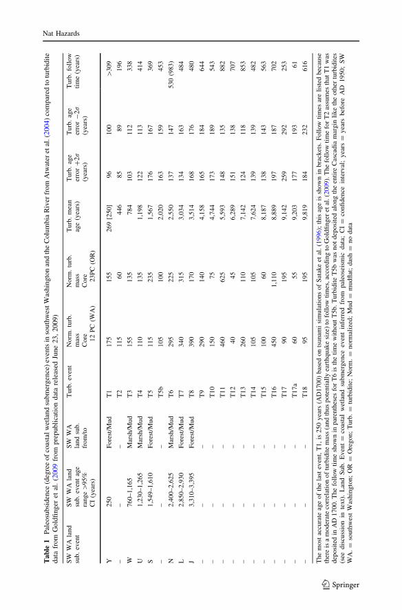
Pal
eosu
bsi
den
ce(d
egre
eo
fco
asta
lw
etla
nd
sub
mer
gen
ce)
even
tsin
sou
thw
est
Was
hin
gto
nan
dth
eC
olu
mb
iaR
iver
from
Atw
ater
etal
.(2
00
4)
com
par
edto
turb
idit
ed
ata
from
Go
ldfi
ng
eret
al.
(20
09
fro
mp
rep
ubli
cati
on
dat
are
leas
edJu
ne
23
,2
00
9)
SW
WA
land
sub.
even
tS
WW
Ala
nd
sub.
even
tag
era
nge[
95%
CI
(yea
rs)
SW
WA
land
sub.
from
/to
Turb
.ev
ent
Norm
.tu
rb.
mas
sC
ore 12
PC
(WA
)
Norm
.tu
rb.
mas
sC
ore 23P
C(O
R)
Turb
.m
ean
age
(yea
rs)
Turb
.ag
eer
ror
?2r
(yea
rs)
Turb
.ag
eer
ror
-2r
(yea
rs)
Turb
.fo
llow
tim
e(y
ears
)
Y250
Fore
st/M
ud
T1
175
155
269
[250]
96
100
[309
––
–T
2115
60
446
85
89
196
W760–1,1
65
Mar
sh/M
ud
T3
155
135
784
103
112
338
U1,2
30–1,2
65
Mar
sh/M
ud
T4
110
135
1,1
98
122
113
414
S1,5
49–1,6
10
Fore
st/M
ud
T5
115
235
1,5
67
176
167
369
––
–T
5b
105
100
2,0
20
163
159
453
N2,4
00–2,6
25
Mar
sh/M
ud
T6
295
225
2,5
50
137
147
530
(983)
L2,8
50–2,9
30
Fore
st/M
ud
T7
340
315
3,0
34
134
163
484
J3,3
10–3,3
95
Fore
st/M
ud
T8
390
170
3,5
14
168
176
480
––
–T
9290
140
4,1
58
165
184
644
––
–T
10
150
75
4,7
44
173
189
543
––
–T
11
460
625
5,5
93
148
135
882
––
–T
12
40
45
6,2
89
151
138
707
––
–T
13
260
110
7,1
42
124
118
853
––
–T
14
105
105
7,6
24
139
139
482
––
–T
15
100
60
8,1
87
138
143
563
––
–T
16
450
1,1
10
8,8
89
197
187
702
––
–T
17
90
195
9,1
42
259
292
253
––
–T
17a
60
55
9,2
03
177
193
61
––
–T
18
95
195
9,8
19
184
232
616
The
most
accu
rate
age
of
the
last
even
t,T
1,
is250
yea
rs(A
D1700)
bas
edon
tsunam
isi
mula
tions
of
Sat
ake
etal
.(1
996
);th
isag
eis
show
nin
bra
cket
s.F
oll
ow
tim
esar
eli
sted
bec
ause
ther
eis
am
oder
ate
corr
elat
ion
of
turb
idit
em
ass
(and
thus
pote
nti
ally
eart
hquak
esi
ze)
tofo
llow
tim
es,
acco
rdin
gto
Gold
finger
etal
.(2
009
).T
he
foll
ow
tim
efo
rT
2as
sum
esth
atT
1w
asdep
osi
ted
inA
D1700.
The
foll
ow
tim
esh
ow
nin
par
enth
eses
for
T6
isth
eti
me
wit
hout
T5b.
Turb
idit
eT
5b
was
not
dep
osi
ted
along
the
enti
reC
asca
dia
mar
gin
like
the
oth
ertu
rbid
ites
(see
dis
cuss
ion
inte
xt)
.L
and
Sub.
Even
t=
coas
tal
wet
land
subm
ergen
ceev
ent
infe
rred
from
pal
eose
ism
icdat
a;C
I=
confi
den
cein
terv
al;
yea
rs=
yea
rsbef
ore
AD
1950;
SW
WA
.=
south
wes
tW
ashin
gto
n;
OR
=O
regon;
Turb
.=
turb
idit
e;N
orm
.=
norm
aliz
ed;
Mud
=m
udfl
at;
das
h=
no
dat
a
Nat Hazards
123

maximum recurrence of the 19 full-margin events (i.e., excluding event T5b) plus the 2rerror in age data. This maximum interval is between events T5 and T6 and equals
*1,300 years, once 2r error is added.
The rupture lengths inferred by Goldfinger et al. (2009) are constrained by the distance
between submarine canyons where turbidites are deposited. In each canyon, completely
unconnected tributary channels have the same number of Holocene turbidites as the main
channel, thus each turbidite is constrained to be synchronous to within several minutes
(Adams 1990; Goldfinger et al. 2003a, 2008, 2009). Only Cascadia earthquakes can produce
this degree of synchronicity (Adams 1990; Goldfinger et al. 2009). Ages of coastal wetland
submergence events in southwestern Washington and the Columbia River from Atwater
et al. (2004) are similar to turbidites, but there is no record in southwestern Washington of a
submergence event or tsunami deposit correlating with the second youngest turbidite, T2.
Also, T2 is one of the smallest margin-wide turbidites, and we suspect that it was not
recorded at many land sites due to minimal coastal subsidence, but at present, we do not
know exactly why there is no record of T2 in southwestern Washington.
We selected recurrences of *300, 525, 750, and 1,300 years of plate convergence to
represent the family of interevent intervals. Figure 2 compares the frequency of turbidite
interevent times relative to these scenario recurrence intervals. The largest mean recur-
rence interval is 983 years, ranging from 660 to 1,287 years at the 2r error level (Table 1;
Fig. 2). The 660–1,287 years range represents the interval between T5 and T6, which was
difficult to constrain tightly (see Goldfinger et al. 2009 for detailed discussion). This
interval excludes turbidite T5b. The presence or absence of T5b at the latitude of Cannon
Beach strongly influences the time-based maximum slip, reducing the largest mean T5–T6
interval from 983 to 530 years (2r range of 220–826 years) (Table 1). However, this
Fig. 2 Frequency of inter-turbidite time intervals (100-years bins) for the last 10,000 years compared to thefour recurrence scenarios (see dotted lines) used for basal branches of the logic tree. Logic tree weightsassigned to each scenario are in parentheses. Illustrated are frequencies for intervals between all 20turbidites (solid bars) and for intervals without turbidite T5b (open bars) relative to cumulative percent ofintervals (lines). The 2r error on the maximum recurrence interval for recurrence data without turbidite T5bis shown encompassing the ‘‘Largest’’ recurrence scenario. Turbidite T5b extends only as far north as 44�N,and may extend as far north as Juan de Fuca Canyon, which includes the latitude of Cannon Beach; the other19 turbidites occur throughout the Cascadia margin
123

illustrates the uncertainties in the time-based model, as T5b was not large enough to be
recorded as a tsunami or coastal subsidence, and therefore probably played a minor role in
strain accumulation during the T5–T6 interval, yet it has a disproportionate effect on our
time-based maximum slip model. A similarly long interval, the time elapsed between T11
and T10, was even more difficult to evaluate because of the difficulty in dating T11. The
T11 event, one of the largest of the Cascadia turbidites, had ubiquitous basal erosion, a
problem common to the largest events, increasing the errors involved in dating and
interpretation of the age. The final average ages and intervals in Goldfinger et al. (2009)
reflect decisions made about which ages for each of these events represent the best quality
results as opposed to the averaged full range of 14C data for each event. In this paper, we
take the conservative approach and use for our ‘‘Largest’’ event a recurrence of
*1,300 years, fitting the outer envelope of the 2r root mean square error of the largest
recurrence. We view using the wider 2r error range as erring on the side of caution,
consistent with standard engineering practice and uncertainties in the age data noted by
Goldfinger et al. (2009). This recurrence translates to a maximum slip of *38 m at the
latitude of Cannon Beach, similar to maximum slip inferred for the 1960 Chile earthquake
(Barrientos and Ward 1990).
4.1.2 Up-dip limit of interplate coupling
We assumed that the most seaward segment of the megathrust will release little coseismic
energy due to velocity-strengthening behavior during rupture of the weakly coupled por-
tion of the outermost megathrust (Wang and Hu 2006; Wang and He 2008). We therefore
tapered slip to zero at the deformation front. Priest et al. (2009) summarize geologic
evidence of weak interplate coupling in the outermost part of the Cascadia megathrust; key
observations include the following:
1. A widespread landward vergent province in Cascadia coinciding with widely spaced,
open folds, suggesting poor interplate coupling (Goldfinger et al. 1992, 1996, 1997;
Mandal et al. 1997), and presence of a mud volcano seaward of the Washington
deformation front (Goldfinger 1994).
2. A well-defined boundary between landward and seaward vergent structures.
3. Change in strike, wedge taper change, and bathymetric break in slope coinciding with
the vergence change.
4. Variable signature of lower plate strike-slip faults that only breach the upper plate in
regions of strong coupling inferred from geologic structure of the upper plate
(Goldfinger et al. 1992, 1996, 1997).
These observations of the Cascadia subduction zone are consistent with the fault slip
model of the Sumatra–Andaman Islands earthquake of December 26, 2004 (Chlieh et al.
2007). Chlieh et al. (2007) also infer decrease in slip up dip from the forearc high into the
outer accretionary wedge (Fig. 3).
4.1.3 Down-dip limit of interplate coupling
The down-dip limit of interplate coupling establishes how far landward the megathrust
rupture and resulting seafloor deformation will reach. In this report, we use published
thermal (Hyndman and Wang 1995; Fluck et al. 1997) and GPS based models (McCaffrey
et al. 2007) and a geologic proxy for down-dip coupling to constrain the down-dip limit of
Cascadia megathrust ruptures. The geologic proxy is a structural transition from
Nat Hazards
123

contraction to extension on the Cascadia margin observable in offshore seismic reflection
data, focal mechanisms and borehole breakouts. We interpret this transition as likely
representing long-term average interplate coupling and note that it is compatible with
thermal and GPS models that cover different time ranges. We tapered slip down dip to
points broadly consistent with this geologic limit or ‘‘stress boundary’’ while still achieving
a best fit to available paleoseismic estimates of coastal subsidence during the AD 1700
earthquake from the Leonard et al. (2004) compilation. The 1700 earthquake in general
appears to be a ‘‘typical’ event based on the turbidite record, and thus may represent an
average rupture scenario. We also did fault model trials to obtain a best match to the
Leonard et al. (2004) data.
Fig. 3 Sumatra forearc shown by single channel profile (A–A0) SEATOS line 1 (taken from Fisher et al.2007). Forearc basin at right, forearc high in center, and subduction thrust (labeled Toe Thrust) and theabyssal plain (Sunda Trench) at left. Lower panel shows preferred slip distribution from Chlieh et al. (2007)for the Sumatra–Andaman Islands earthquake of December 26, 2004, in map view based on GPS data.Profile of the Chlieh et al. (2007) slip distribution along cross section A–A0 is shown above the SCS (singlechannel seismic) profile. Map location of the subduction zone megathrust on the map is the black line withtriangles pointing down the fault dip; dark gray lines to the east are depth contours on the megathrust.Contours in shades of gray on lower map are inferred coseismic slip; arrows show direction and magnitudeof observed and modeled coseismic and post-seismic slip, as indicated in the map legend
123

While there is no certainty that the mapped pattern of contractional and extensional
structures actually reflects plate coupling, observations of the 2004 and 2005 earthquakes
in Sumatra suggest that this may be the case. Models of the Sumatra slip distribution such
as those derived from GPS (Chlieh et al. 2007; Fig. 3) and seismologically (Ammon et al.
2005) suggest that the down-dip extent of seismogenic slip roughly corresponds to the
transition from the arcward part of the forearc high to the lightly deformed forearc basin
(Goldfinger and McNeill 2006). A review of less well-recorded great earthquakes such as
Kamchatka (1952), Alaska (1964), and Chile (1960) yields ambiguous interpretations,
slightly favoring a similar interpretation (Goldfinger et al. 2007). The 1960 Chile earth-
quake may be an exception, because there is some evidence that it ruptured beneath the
forearc basin (Barrientos and Ward 1990).
In Cascadia, we map a transition similar to that of Sumatra based on the following
observations:
1. The Cascadia forearc high is probably an area of contraction and thus high
compressional stress, since the high consists of seaward vergent thrust faults in an
imbricate stack (Fig. 4). These faults also form the western limb of the forearc basin
and are observed as flexural slip faults developed within stratigraphic horizons of the
forearc basin stratigraphy (Fig. 4).
2. Forearc basins are probably areas of extension and low compressional stress, since, as
shown in the Fig. 4, contractional deformation of the basin is limited to the western
edge, gives way to relatively undeformed stratigraphy in the basin center and landward
limb.
3. The change from contractional to extensional structures across the seaward limbs of
the forearc basins forms a regular pattern (Fig. 5). We used the youngest structures
available, though only approximate temporal control is available from a few test wells
(McNeill et al. 2000). Note that evidence of extension of the Washington shelf shown
in Fig. 5 as a cluster of white dots corresponds to shallow listric normal faulting
(McNeill et al. 1997) and is probably not relevant to coupling on the megathrust.
4. Earthquake focal mechanisms (Global Centroid Moment Tensor Database 2007; Trehu
et al. (2008), and various sources) and borehole breakout data (Werner et al. 1991)
indicate a change in compressional axis from convergence-parallel (northeast) to arc-
parallel (north–south) at approximately the boundary between contractional to
extensional forearc structures (Fig. 5).
Fig. 4 Cross section across Heceta Bank, Oregon from Chevron line HOG 15 and Western Geco lineWO-18. This typical forearc section shows the compressional nature of the forearc basin (contrast withsection of Wells et al. 2003, along the same profile). Flexural slip faulting controls the basin western margin,the eastern margin is undeformed or extensional. Boundary between extension and compression is mappedfor numerous similar profiles in Fig. 5. See Fig. 5 for location of this cross section. Unit Tsr is Siletz RiverVolcanics of the Siletzia terrane considered to be a hard rock backstop in contact with sedimentary rocks ofthe accretionary prism (bedded units) to the west. Twt is two-way travel time
Nat Hazards
123

5. The stress boundary in Fig. 5 is compatible with other down-dip estimates of coupling
based on thermal models (Hyndman and Wang 1995; Fluck et al. 1997), leveling data
(Mitchell et al. 1994; Schmidt et al. 2007; Burgette et al. 2009) and GPS data
(McCaffrey et al. 2007).
Each of these indicators cannot strictly be compared to the others as they represent
different physical properties and different time scales. Nevertheless, the combined data are
quite consistent and seem to represent a coherent transition from convergence-related
Fig. 5 Compilation of geologic stress indicators along the central Cascadia margin. Dark gray dots showcompressive structure locations, white dots show extensional structures mapped along multichannelreflection profiles. Gray arrows with white outlines show P-axes from borehole breakouts, Black circles withwhite axes show P-axes from focal mechanisms from the Global Centroid Moment Tensor Database. Blackdotted contours show geodetic uplift contours of Mitchell et al. (1994). Three structural uplifts known asNehalem Bank (NB), Heceta Bank (HB), and Coquille Bank (CB) shown as light gray polygons with whiteoutlines. Bold dashed line shows mean stress transition (‘‘stress line’’) from compressive to extensionalindicators. See text and Priest et al. (2009) for data source references
123

compression to arc-parallel compression that is well known in the Cascadia forearc (Wang
and He 1999).
4.1.4 Interplate coupling at forearc basins and banks
The stress boundary shown in Fig. 5 (supported by leveling and tide gauge data) suggests
that broad regions of the upper plate where the stress line swings landward coincide with
major structural uplifts. The central Oregon region where the stress line swings seaward
coincides with a deep structural and gravity low (McNeill et al. 2000). In Oregon, two of
the structural uplifts correspond to free-air gravity highs and are known as Coquille, and
Heceta Banks, while the third Nehalem Bank, is a gravity low (Fig. 5; see gravity map of
Wells et al. 2003). We suggest that the map pattern of inferred higher coupling corre-
sponding to the submarine banks may indicate regions of high slip during subduction
earthquakes because the GPS and leveling data suggest greater present interseismic elastic
strain that must be released in earthquakes, while the stress line indicates greater long-term
strain. This pattern is clearly apparent in Sumatra, where the 2007, 2005, and 2004 rupture
patches were for the most part centered over analogous structural highs, tapering landward
into the undeformed forearc basin, and seaward into the outer wedge (Chlieh et al. 2007;
Konca et al. 2008).
Wells et al. (2003) suggest an alternative model. They argue on the basis of global
comparisons of earthquake slip models with gravity data, that seismic moment is con-
centrated beneath forearc basins. While this model appears to work well for several well-
known cases such as Nankai and Chile, it failed to predict the Sumatra 2004 distribution of
slip or slip distributions of the other largest known earthquakes such as Kamchatka (1952)
and Alaska (1964). The basin model proposed by Wells et al. (2003) is also incompatible
with the structural data outlined earlier as it requires the forearc basins to be fully
extensional features. A related model by Song and Simons (2003) suggests that slip is
concentrated in trench-parallel gravity lows, a proposal similar to but distinct from that of
Wells et al. (2003). Though these models are commonly linked, the Song and Simons
model subtracts an average gravity profile, and identifies lows from the resulting data,
something not done in the Wells et al. model. The Song and Simons model also fails to
predict slip distributions in Sumatra.
At present, it is not possible to determine which of these models, if any, is operative in
Cascadia. We produced simulations of coseismic deformation for both basin and bank slip
patch models but give less weight in our decision tree to the basin model.
4.1.5 Splay fault
Common along subduction margins with thick incoming sedimentary sections is a major
splay fault that separates the active accretionary wedge from an older accretionary com-
plex. These splay faults may have also generated tsunamis or contributed to tsunami
generation during subduction zone earthquakes (e.g., Plafker 1972; Park et al. 2002).
Along the central Cascadia margin (*45�N to 47�N), this fault is well expressed and
marks the boundary between the low tapering lower slope wedge and steeper tapering
upper slope and shelf accretionary complex (Figs. 6, 7). On a northern Oregon proprietary
profile and on depth-migrated Sonne lines 103 and 108 (Adam et al. 2004), the approxi-
mate fault dip is *30�. Some profile crossings such as that of Fig. 7 suggest recent
seafloor offset, and thus recent fault activity.
Nat Hazards
123

Given the evidence for recent movement, the clear domain boundary between older and
younger accretionary complexes, and the structural indications of a significant difference in
deformation style, we infer that the Cascadia splay fault is a significant structure capable of
diverting slip from the decollement to the surface as has been suggested for the Nankai
margin (Cummins et al. 2001). We use a generalized fault deformation model of this fault
(Fig. 1) to explore the effect on tsunami runup and inundation.
4.2 Cascadia fault rupture simulation
All simulations of surface deformation from Cascadia fault rupture scenarios employ the
point source solution from Okada’s (1985) dislocation model and emulate coseismic
deformation between 43.9�N near Florence, Oregon to *47.9�N at Neah Bay, Washington
(Fig. 1). Compared to the importance of and large uncertainties in the slip distribution,
Fig. 6 Shaded bathymetry of the Oregon margin, with structural map overlain (Goldfinger 1994). Thelower slope (medium gray with rough topography) is characterized by (1) landward vergence; (2) lowsurface taper (profile E–E0); (3) wide fold spacing and is dominated by margin parallel folds. Olderaccretionary complex (lighter gray to the east) is dominated by convergence-normal fold trends landwardvergence, and steep mid-slope defining a steeper wedge taper. The two provinces are separated by a seawardvergent splay fault (bold gray lines with triangles pointing down the thrust fault dip) and abrupt break insurface slope. Mapped traces of the splay fault scarps are shown in this figure; generalized location of themodel fault used for the tsunami source models is depicted on Fig. 1. Splay fault is imaged by USGSreflection profile L-5-WO77-12, shown in Fig. 7. Bathymetric profile (profile E–E0) with verticalexaggeration of 1:16.7 shows low surface wedge taper, and steep upper slope separated by the splayfault scarps. See Fig. 1 for location of this map
123

other factors such as material heterogeneity, inelastic behavior, dynamic deformation, and
horizontal seafloor motion are of secondary concern. Therefore, the model of a uniform
elastic half-space with a Poisson’s ratio of 0.25 is employed in this work. Attention is paid
mainly to the most critical issue of how to assign coseismic slip along the Cascadia
megathrust.
Slip direction of the coseismic rupture is assumed to be exactly opposite of plate
convergence. The plate convergence direction and rate are calculated from Euler vectors as
explained in Wang et al. (2003) and account for convergence between the Juan de Fuca
Plate and the North American Plate, including reduction of convergence by forearc rotation
(McCaffrey et al. 2000, 2007).
Megathrust geometry is modified from that of McCrory et al. (2004). In the McCrory
et al. (2004) model, because depth is measured from sea level, the depth of the megathrust
is over 5 km at the deformation front, where the actual water depth to the seafloor is
2–3 km. To let the upper surface of the elastic half-space approximately represent the
seafloor, the most up-dip part of the megathrust is ‘‘raised’’ to 2–3 km depth by resetting
the 5-km slab surface contour of McCrory et al. (2004) (located seaward of the deformation
front) to 2 km. This ‘‘raised’’ structure contour line and other contour lines of McCrory
et al. (2004) at 5 km intervals are used to construct the megathrust geometry using GMT
program ‘‘Surface.’’
All of the fault ruptures are simulated utilizing the slip function of Wang and He (2008)
modified from the fb76 slip distribution of Freund and Barnett (1976). Fundamental to the
Wang and He (2008) approach is recognition that the seismogenic zone of subduction
faults has an up-dip limit, seaward of which the fault exhibits velocity-strengthening
behavior. This view is supported by observed and inferred coseismic seafloor deformation
of great subduction zone earthquakes, particularly that associated with the 2004, 2005, and
2007 Sumatra events (Fig. 3). Therefore, all rupture simulations incorporate coseismic slip
tapering to zero at the deformation front. In a real megathrust earthquake, the slip varies
Fig. 7 Unmigrated USGS reflection profile L-5-WO77-12 across the mid-slope off north-central Oregon.Splay fault separating young wedge (west) from older accretionary complex (east) is imaged as a zone withtwo major traces and active upward branches (Mann and Snavely 1984). Young basin fill is deformed by theupward branching fault, and upper trace breaks the seafloor at this location. Lower slope is characterized bya more open fold style, and landward vergence indicative of less interplate coupling than the upper slopeseaward vergent fold and thrust belt. See Fig. 6 for location and further depiction of vergence changes. SWis southwest; NE is northeast
Nat Hazards
123

tremendously along strike giving rise to the concept of asperities. Because we cannot
predict where the maximum slip will occur along strike, we use a ‘‘regional slip patch’’
model to simulate an average uniform scenario. Local slip patches are assumed to be at
either basins or banks and are simulated by quadratically scaling maximum slip with down-
dip and up-dip patch width. Each assumed slip distribution on the megathrust for splay
fault models is simply truncated at the surface trace of the splay fault. Figure 8 shows
boundaries of the simulated splay fault, local basin and bank slip patches, and the regional
slip patch. The down-dip boundary of the regional slip patch was constrained by both the
previously discussed ‘‘stress boundary’’ and by a best fit to available coseismic subsidence
data of Leonard et al. (2004). We found that use of seaward skew (q = 0.3) for regional
slip patches produced a somewhat poorer fit than symmetrical slip (q = 0.5) to onshore
paleoseismic estimates of coseismic subsidence, as did varying the rupture width by 20 km
(Fig. 9).
4.3 Logic tree evaluation of Cascadia earthquake source parameters
The parametric analysis of tsunami sources was guided by a logic tree with branches
arranged from most to least important controls on vertical coseismic deformation for
Cascadia earthquakes (Fig. 10). The four earthquake source parameters chosen, from most
to least important, are
1. Earthquake size (coseismic slip)
2. Presence or absence of a splay fault
Fig. 8 Structural boundaries relevant to this work. Thin lines are depth contours at 10 km intervals to theCascadia megathrust. Large triangles are the surface trace of the megathrust (up-dip edge of regional slippatches); small triangles are the model splay fault; basin slip patch is the hachured line; bank slip patch isthe bold black line; the ‘‘stress line’’ where crustal contraction changes eastward to crustal extension is thedashed white line; modeled down-dip extent of regional slip patches is indicated by the dotted white line
123

3. Fault rupture extent (regional rupture or local basin/bank rupture), and
4. Slip distribution (symmetrical within banks or basins and symmetrical or seaward
skewed within regional slip patches).
Weighting factors were assigned by the scientific team (authors of this paper) to each
branch of the logic tree based on consensus and observational geologic data at Cascadia
and other potentially analogous subduction zones. Therefore, weights represent the relative
confidence or preference of the scientific team. The weights do not reflect the temporal
Fig. 9 Coastal subsidence predicted by buried rupture, regional slip patch models utilizing 500 years of sliprelease and comparison with AD 1700 coseismic subsidence data The approximate mean recurrence ofCascadia earthquakes is 500 years. Square and large circles indicate best quality and better quality data asexplained in Leonard et al. (2004). Models utilize a symmetric slip distribution but vary rupture width by±20 km from the best fit width to geologic data; bold line = preferred medium-width rupture patch), dottedline = 20 km narrower, and thin line = 20 km wider. To test for sensitivity of tsunami simulations toseaward-skewed (SS) slip (q = 0.3), one model was constructed utilizing a medium patch width (dashedline)
Fig. 10 Logic tree for selection and relative weighting of Cascadia tsunami sources. See the text andTables 2 and 3 for detailed summaries of the weighting factors for all branches
Nat Hazards
123

probability of the next tsunami. Table 2 shows a summary of the weighting factors and
reasons for the weights. Table 3 summarizes all Cascadia scenarios and their logic tree
weights. Figure 11 illustrates map views of the eight coseismic deformation scenarios for
slip equaling 525 years of plate convergence (our ‘‘Average’’ scenarios in the logic tree).
In order to save computational time and avoid simulating many small events with
similar, small inundations, we utilized only one of the eight ‘‘small’’ earthquake sources for
slip equaling *300 years of plate convergence, Small 9; hence, we used only 25 of the 32
Cascadia scenarios. Small 9 had the highest logic tree weight for the ‘‘small’’ branch and
consisted of a regional slip patch with symmetric slip and no splay fault (buried rupture on
the megathrust). For relative hazard computations, we assigned all eight of the ‘‘small’’
logic tree weights to this one scenario, increasing its weight from 0.072 to 0.25 (Table 3).
Table 2 Explanation of logic tree weights
Coseismic slip Each scenario is assigned a weight according to the numberof earthquakes of a particular size that are recorded in the*10,000-year record of 20 Cascadia turbidites. For dataavailable in 2007, a weight of 0.05 applies to the ‘‘largest’’slip, because one of the 20 events had an interseismicinterval of *1,300 years; 3 of 20 events were ‘‘large’’events assigned a weight of 0.15; 11 out of 20 weremoderate in size, or ‘‘average’’ events assigned a weight of0.55; and 5 of 20 were considered ‘‘small’’ events andweighted at 0.25.
Slip partitioned to a splay fault Weighting factors assigned in this branch reflect greaterlikelihood that larger slip events will trigger coseismic slipon a splay fault. For the ‘‘largest’’ and ‘‘large’’ scenarios,the ratio of weights assigned to splay fault versus buriedrupture events is 0.8:0.2. For ‘‘average’’ scenarios, the ratiois 0.6:0.4. For ‘‘small’’ events, the ratio is the opposite ofthat used for the largest scenarios, or 0.2:0.8
Rupture model The regional slip patch model was assigned a higher weight(0.6) than local ruptures in forearc basins and banks (0.4),because (1) the trench-parallel length of local slip patches ishighly uncertain, whereas the regional slip patchsubstantially includes all local slip patches; (2) turbiditedata are consistent with long ruptures as the primary rupturetype experienced in the northern Cascadia margin(Goldfinger et al. 2008); and (3) landward extent of theregional slip patch is constrained by the ‘‘stress line’’ ofFig. 5 and to consistency with paleoseismic estimates ofcoseismic subsidence (Fig. 9)
Slip distribution: basin versus bank slippatches
Higher weight (0.7) to slip patches concentrating slip atforearc banks versus forearc basins (0.3), because mappedstructures within the banks are contractional, indicatinggreater strain accumulation possibly linked to strongcoupling on the locked zone beneath the banks. Structuresunder the centers and landward limbs of basins areextensional indicative of lesser strain accumulation fromthe megathrust locked zone (see text for discussion)
Slip distribution for regional slip patches:symmetric versus seaward skewed
The symmetric slip distribution (weight of 0.6) was judgedmore likely than the seaward-skewed slip (weight of 0.4),because the skewed distribution results in poorer fit tocoastal paleosubsidence data of Leonard et al. (2004) forthe 1700 AD Cascadia event (Fig. 9)
123

Table 3 Earthquake source parameters and weighting factors used in logic tree. Slip listed in the table ismaximum slip for each slip distribution and is estimated for the latitude of Cannon Beach
Rupturescenario
Slip(m)
Mw Splay fault/buried rupture
Rupturemodel
Slip distribution Total weightfactor
Largest 1 (0.05) *38 *8.8 Splay (0.8) Local (0.4) Offshore bank (0.7) 0.011
Largest 2 (0.05) *38 *8.8 Splay (0.8) Local (0.4) Offshore basin (0.3) 0.005
Largest 14 (0.05) *38 *9.2 Splay (0.8) Regional(0.6)
Symmetric (0.6) 0.014
Largest 12 (0.05) *38 *9.2 Splay (0.8) Regional(0.6)
Seaward skew (0.4) 0.010
Largest 6 (0.05) *38 8.8 Buried rupture (0.2) Local (0.4) Offshore bank (0.7) 0.003
Largest 7 (0.05) *38 8.8 Buried rupture (0.2) Local (0.4) Offshore basin (0.3) 0.001
Largest 9 (0.05) *38 9.3 Buried rupture (0.2) Regional(0.6)
Symmetric (0.6) 0.004
Largest 10 (0.05) *38 9.3 Buried rupture (0.2) Regional(0.6)
Seaward skew (0.4) 0.002
Large 1 (0.15) *22 *8.6 Splay (0.8) Local (0.4) Offshore bank (0.7) 0.034
Large 2 (0.15) *22 *8.6 Splay (0.8) Local (0.4) Offshore basin (0.3) 0.014
Large 14 (0.15) *22 *9.1 Splay (0.8) Regional(0.6)
Symmetric (0.6) 0.043
Large 12 (0.15) *22 *9.1 Splay (0.8) Regional(0.6)
Seaward skew (0.4) 0.029
Large 6 (0.15) *22 8.6 Buried rupture (0.2) Local (0.4) Offshore bank (0.7) 0.008
Large 7 (0.15) *22 8.6 Buried rupture (0.2) Local (0.4) Offshore basin (0.3) 0.004
Large 9 (0.15) *22 9.1 Buried rupture (0.2) Regional(0.6)
Symmetric (0.6) 0.011
Large 10 (0.15) *22 9.1 Buried rupture (0.2) Regional(0.6)
Seaward skew (0.4) 0.007
Average 1 (0.55) *15 *8.5 Splay (0.6) Local (0.4) Offshore bank (0.7) 0.092
Average 2 (0.55) *15 *8.5 Splay (0.6) Local (0.4) Offshore basin (0.3) 0.040
Average 14 (0.55) *15 *9.0 Splay (0.6) Regional(0.6)
Symmetric (0.6) 0.119
Average 12 (0.55) *15 *9.0 Splay (0.6) Regional(0.6)
Seaward skew (0.4) 0.079
Average 6 (0.55) *15 8.5 Buried rupture (0.4) Local (0.4) Offshore bank (0.7) 0.062
Average 7 (0.55) *15 8.5 Buried rupture (0.4) Local (0.4) Offshore basin (0.3) 0.026
Average 9 (0.55) *15 9.0 Buried rupture (0.4) Regional(0.6)
Symmetric (0.6) 0.079
Average 10 (0.55) *15 9.0 Buried rupture (0.4) Regional(0.6)
Seaward skew (0.4) 0.053
Small 1 (0.25) *8 *8.3 Splay (0.2) Local (0.4) Offshore bank (0.7) 0.000 [0.014]a
Small 2 (0.25) *8 *8.3 Splay (0.2) Local (0.4) Offshore basin (0.3) 0.000 [0.006]a
Small 14 (0.25) *8 *8.9 Splay (0.2) Regional(0.6)
Symmetric (0.6) 0.000 [0.018]a
Small 12 (0.25) *8 *8.9 Splay (0.2) Regional(0.6)
Seaward skew (0.4) 0.000 [0.012]a
Small 6 (0.25) *8 8.3 Buried rupture (0.8) Local (0.4) Offshore bank (0.7) 0.000 [0.056]a
Small 7 (0.25) *8 8.3 Buried rupture (0.8) Local (0.4) Offshore basin (0.3) 0.000 [0.024]a
Nat Hazards
123

4.4 Distant tsunami sources
We investigated two distant tsunami scenarios in order to simulate the largest historical
event and a hypothetical maximum-considered event; both tsunamis are triggered by Mw of
*9.2 earthquakes in the Gulf of Alaska (Figs. 12, 13). The vertical deformation inferred
by Johnson et al. (1996) provided the initial condition for simulation of the largest his-
torical event, the 1964 Prince William Sound earthquake (Fig. 12). The maximum-con-
sidered event is the hypothetical Source 3 of the TPSW (2006) that in their investigation
caused the largest distant tsunami at Seaside, Oregon, 9 km north of Cannon Beach
(Fig. 1). This source has four segments with 15, 20, 25, and 30 m of slip (see TPSW’s
Table 6, p. 41) and maximum uplift over twice as high as that inferred for the 1964
earthquake (Figs. 12, 13). This large uplift is in a relatively narrow ‘‘spike’’ near the
surface trace of the fault and is caused by a singularity in the Okada (1985) uniform slip
model (Vasily Titov 2008, personal communication). According to Titov (2008, personal
communication) the ‘‘spike’’ has little effect on the resulting tsunami relative to the broader
area of 3–5 m uplift to the northwest. TPSW (2006) concluded that better directivity to the
northern Oregon coast causes the larger size of this tsunami relative to the 1964 event.
4.5 Hydrodynamic tsunami modeling
Vertical components of deformation from the 25 Cascadia and the two Alaska earthquake
sources were used as instantaneous static deformations for tsunami simulations. The finite
element model SELFE (Zhang and Baptista 2008) simulated propagation and inundation
with an unstructured numerical grid utilizing post-earthquake topography. Grid spacing for
simulation of local Cascadia sources varied from 200 m at the source to 2.2 m in parts of
Cannon Beach with detailed topographic data (Figs. 14, 15). Deep ocean propagation of
the two distant tsunamis utilized grid spacing on the order of 11 km. Each Cascadia
simulation was run for at least 2 h of ‘‘tsunami time.’’ Some simulations were run longer
(up to 8 h of ‘‘tsunami time’’) in order to check the importance of inundation from later
Table 3 continued
Rupturescenario
Slip(m)
Mw Splay fault/buried rupture
Rupturemodel
Slip distribution Total weightfactor
Small 9 (0.25) *8 8.9 Buried rupture (0.8) Regional (0.6) Symmetric (0.6) 0.250 [0.072]a
Small 10 (0.25) *8 8.9 Buried rupture (0.8) Regional (0.6) Seaward skew (0.4) 0.000 [0.048]a
Slips at other latitudes vary from these values according to estimates of plate convergence rate from theEuler pole of Wang et al. (2003). Convergence rate used to estimate slip for this table is 28.9 mm/year, theappropriate value at the latitude of Cannon Beach. Mw values are calculated assuming rigidity of 40 GPa,the appropriate slip distribution for each source scenario, and maximum slip determined from plate con-vergence assuming complete coupling. Areal extents assumed in Mw calculations for basin and bank slippatch sources are given in Fig. 11; areal extent for regional slip patch sources are assumed to be the entiremargin. Symbol *means Mw estimated rather than calculated based on similarity of slip amount betweensplay fault and buried rupture sources and narrower east–west extent of splay fault slip patches relative toburied ruptures
Note: numbers in parentheses are weighting factors assigned to individual branch parameters. In each row,the product of the four weights is equal to the total weighting factor used for the earthquake source scenarioa Weighting factors in brackets were assigned to ‘‘small’’ scenarios in the initial logic tree (32 branches).The final logic tree (25 branches) assigned a single weight equal to the sum of all small scenario weights to‘‘Small 9’’
123

refracted waves or to accommodate propagation from the two distant tsunami sources in
Alaska. An 8-h simulation of a Cascadia source revealed that wave height decreased
significantly after 2 h, so later arriving waves were smaller and did not ‘‘stack’’ in low-
lands; hence, 2 h of ‘‘tsunami time’’ was simulated for most Cascadia sources.
4.6 Tides
All simulations in this investigation were run at 2.711 m above geodetic mean sea level
NAVD 1988 based on mean higher high water (MHHW) at the Astoria, Oregon tide gauge.
Neglecting non-linear effects, the TPSW (2006) did a probabilistic analysis of tides for
Seaside, Oregon and concluded that the effect of tides for a 500-year Cascadia tsunami
decreased open coastal run-up by 0.7 m from their assumption of tide at mean high water.
Fig. 11 Vertical coseismic deformation patterns for release of 525 years of convergence on the Cascadiasubduction zone. White numbers are deformation in meters, positive = uplift; negative = subsidence;contours are at 0.5 m. Bank slip patch models place slip under submarine banks; basin models undersubmarine basins; slip is quadratically scaled to the width of the basin or bank. Regional slip patch modelsplace slip west of the ‘‘stress line’’ in Figs. 5 and 8 in either a symmetric (q = 0.5) or seaward-skewed(q = 0.3) distribution. Splay fault scenarios cut off the slip distribution at the splay fault, amplifying upliftfrom increase of fault dip to 30�
Nat Hazards
123

Fig. 12 Coseismic deformation from the 1964 Prince William Sound earthquake from Johnson et al.(1996); Negative numbers = meters coseismic subsidence; positive numbers = meters coseismic uplift.Shown for comparison is the area of uplift from the theoretical maximum-considered distant tsunami sourceof Fig. 13
Fig. 13 Maximum-considered distant tsunami source from the TPSW (2006) analysis for Seaside, Oregon;Negative numbers = meters coseismic subsidence; positive numbers = meters coseismic uplift. Shown forcomparison is the area of uplift from the 1964 Mw 9.2 earthquake (Fig. 12)
123

Our assumption of MHHW for the Cascadia tsunami simulations is therefore conservative.
This tide is *0.3-m higher than the tide during initial arrival of the 1964 tsunami from
Prince William Sound (Priest et al. 2009).
4.7 Comparison of simulated tsunamis to observations
Distribution of three prehistorical (paleotsunami) deposits and observations of historical
tsunami inundation from the 1964 tsunami from Witter (2008) served as ground truth
checks of the tsunami modeling approach. Inland reach of paleotsunami deposits marks the
minimum inundation of Cascadia tsunamis. Ages of the three deposits from Witter (2008)
Fig. 14 Unstructured computational grid used in tsunami simulations. The left panel shows the full grid andthe right is a zoom-in near the Ecola Creek. BC = British Columbia; CB = Cannon Beach
Fig. 15 Grid resolutionexpressed as the equivalentradius of each numerical gridelement plotted againstbathymetric depth [negativedepths are above mean higherhigh (MHHW)]. Graphdemonstrates that resolutionchanges gradationally from tensof kilometers in the deep ocean toa few meters on land
Nat Hazards
123

allowed comparison of relative size of earthquakes to relative inundation. Match of sim-
ulated inundation, run-up, and flow depths to observations of the tsunami from the 1964
Prince William Sound earthquake tested accuracy of the hydrodynamic model and inputs.
Tsunami simulations used as inputs digital elevation models of the modern topography for
the 1964 simulation and prehistorical landscapes for paleotsunami simulations.
4.8 Reconstructing the prehistorical landscape
A 1,000-year B.P. (before AD 1950) landscape (digital elevation model) was constructed
by removal of artificial fills from the modern landscape and inferring the paleolandscape
from analysis of coastal erosion data, and cores. One thousand years corresponds
approximately with the age of the Cascadia tsunami deposit that reaches furthest inland of
the three deposits mapped in the Ecola Creek valley by Witter (2008). The landscapes were
reconstructed by:
1. Increasing relief on the Ecola Creek valley by *1 m, based on the observation that sea
level *1,000 years ago was *1 m lower (Witter 2008) and that sedimentation in
coastal Oregon estuaries keeps up with rising sea level.
2. Moving the shoreline at sedimentary rock bluffs and attached sand spits 70 m seaward
to account for 1,000 years of erosion. The erosion rate was estimated from historical
rate data of Allan and Priest (2001) and of Priest and Allan (2004); see details of the
calculation in Priest et al. (2009).
3. Constructing two landscapes, one with foredune height the same as present, and one
with no barrier dune fronting the estuary.
4.9 Comparison of simulated coseismic deformation to observations
Another means of testing validity of the simulations is to compare simulated coseismic
subsidence for Cascadia scenarios to subsidence estimated from paleosubsidence data. We
used data compiled by Leonard et al. (2004) and Nelson et al. (2008) for the AD 1700
*Mw 9 Cascadia earthquake (Satake et al. 2003), an ‘‘average’’ event in terms of turbidite
mass and thickness (proxies for earthquake size) compared to other turbidites in the
10,000-year record (Table 1; Goldfinger et al. 2009; Priest et al. 2009).
5 Results
5.1 Cascadia earthquake sources
Modeled coseismic uplift from the 25 Cascadia source scenarios ranged from nearly 17 to
*2 m at the latitude of Cannon Beach (Fig. 16). We also simulated inundation from the 12
Cascadia sources of the TPSW (2006) (Fig. 16). Tsunami simulations thus totaled 37 and
utilized post-earthquake topography to estimate inundation.
5.2 Cascadia tsunami inundation and water elevation
Tsunami water elevation at the shoreline (Figs. 17, 18) and inundation (Figs. 17, 19, 20)
are plotted in terms of cumulative logic tree weights in order to illustrate relative confi-
dence that each scenario covers all potential variability for Cascadia tsunamis. Logic tree
123

weights were summed for overlapping inundations, subtracted from 1 and multiplied by
100 to get percent confidence. We plotted results for the TPSW sources by making the ad
hoc assumption that all have equal logic tree weights within their stochastic framework.
TPSW tsunamis were larger than most of ours, overlapping our events at[95% confidence
level (Figs. 18, 19, 20).
Water depth at the open coast for our scenario tsunamis varied from 3 to 18 m at a
representative observation point (Fig. 18), while inundation varied from *1.5 to 3.8 km in
the lowest valley at Ecola Creek (Fig. 19). Runup was amplified by up to 40% at near-
shore bathymetric lows, especially if combined with U- or V-shaped valleys where the
*30 m contour penetrates\1 km inland (Figs. 17, 21). Maximum open coastal runup was
30.3 m in the Tolovana area. Cascadia sources of the TPSW (2006) reached a maximum
runup of 34.7 m in the same area.
Some regional slip patch sources produced inundation matching key confidence limits
(Fig. 20). A summary of runup for key source scenarios designated by their names in the
Fig. 16 West-to-east cross sections of coseismic deformation for all Cascadia earthquake source scenarios.Cross sections extend from the deformation front to the shoreline at Cannon Beach. The final 25 tsunamisources utilized by Oregon Department of Geology and Mineral Industries (DOGAMI) for this investigation(bold lines) have major uplift mostly landward (east) of stochastic scenarios developed by USGS for TPSW(2006) (thin gray lines). Scenarios with decreasing deformation have decreasing fault slip at values of *38,22, and 15 m with one source scenario, Small 9, at *8 m. Titles on each graph explain the type of slipdistribution used; see also the logic tree (Fig. 10) for explanation of source scenario names in each legend
Nat Hazards
123

logic tree is given here. Approximately matching isolines of percent confidence are also
listed next to each scenario name. Runup elevations are representative of most open coastal
sites in the study area with maximum values in parentheses:
• Largest 14 (*99% isoline): *20 m runup (30.3 m)
• Large 14 (*90% isoline): *13 m runup (15.9 m)
• Average 14 (*70% isoline, preferred scenario): *10 m runup (12.2 m)
• Average 9 (*50% isoline): *8 m runup (9.4 m)
• Small 9 (*6–10% isolines): *5.5 m (6.1 m)
These regional slip patch scenarios should produce inundation at approximately these
confidence limits in areas north and south of Cannon Beach, because source deformation is
similar. Inundation and open coastal wave elevation from the preferred source scenario,
Average 14, closely tracks both the 70% confidence limit and the regulatory inundation
line (Olmstead 2003) established by Oregon in 1995 (Priest 1995; Figs. 18, 19, 20). Less
accurate 1995 topographic data and lack of numerical modeling in 1995 of dry land
inundation probably caused most of the differences between the Average 14 and regulatory
inundation, because the two simulations have similar tsunami elevations at the open coast.
Fig. 17 Observation lines and points for inundation, maximum wave elevations, and time histories of wavearrivals. Solid white observation line for maximum wave elevation data approximates the limit of inundationon steep slopes at the open coast; dashed white observation line approximates the shoreline (0.0 mNAVD88). Thin black lines illustrate water depth in 2-m intervals; labels on depths are relative to theNAVD88 datum
123

5.3 Effect on inundation and runup of slip, splay faulting, and slip patches
Slip magnitude was the most important control of inundation and runup, both of which
increased linearly with slip (Fig. 22). The next largest differences between scenarios were
caused by increasing uplift through splay faulting and distributing slip into regional versus
local bank or basin slip patches (Fig. 23; Table 4). Local basin slip patches produced much
smaller runup and inundation relative to all other sources (Table 4), because the nearest
basin is *100 km south of Cannon Beach (Fig. 8).
While the splay fault amplified tsunamis relative to buried rupture sources, the trun-
cation of slip distributions at the surface trace of the splay caused the degree of amplifi-
cation to decrease as more of the slip distribution was seaward of the splay (Fig. 23).
Amplification by splay faulting was 6–31% for tsunami water level at the open coast and
2–20% for inundation up Ecola Creek (Fig. 23). Amplification was negligible for basin slip
patches, owing to negligible slip in deep water. For sources with significant slip, ampli-
fication was largest for symmetrical regional slip patches, followed by bank slip patches,
and least for seaward-skewed regional slip patches (Fig. 23).
5.4 Alaska 1964 tsunami simulation
Simulated open coastal runup for the 1964 Alaska tsunami was mostly *6.5 m with a
maximum of 8.2 m where the wave was funneled into the mouth of Ecola Creek. Flow
depth and inundation from the simulation closely matched observations gleaned from
Fig. 18 Cumulative percent confidence that tsunami water depth will be less than the scenario depth for aCascadia tsunami (*500-years event). Average 14 is the preferred scenario that received the highest logictree weight for the full 32-scenario analysis. Water depths of the maximum distant tsunami scenario (Source 3of TPSW 2006), the 1964 Alaska distant tsunami, tsunami water elevation for the Oregon Department ofGeology and Mineral Industries (DOGAMI) regulatory zone (Priest 1995; Olmstead 2003), and tide assumedfor all simulations are shown for comparison. Included for comparison are data for the 12 stochastic sourcesutilized by the TPSW (2006); each is assumed to have one-twelfth of the total logic tree weight of 1.0. Note:TPSW water depths shown by open squares are inferred from results of an earlier version of the SELFEhydrodynamic model compared to four 2008 simulations (solid squares). All tsunami water depths are from apoint located on the open coastal shoreline at 123.966586� West Longitude, 45.891190� North Latitude atapproximately 0.0 m elevation NAVD88 (water level observation point in Fig. 17)
Nat Hazards
123

historical records (Witter 2008) (Table 5; Fig. 24). The Bell Harbor Motel and the Steidel
House had particularly high quality observational data (Witter 2008) and the best match of
simulation to observations (Table 5). Match to observed inundation was improved in two
trials by refining the part of the numerical grid defining the Ecola Creek channel and
highway embankments. In front of the foredune in downtown Cannon Beach, the 1964
tsunami runup reached an estimated elevation of 6.1 m (NAVD88); the simulation pre-
dicted 6.7 m. Simulated inundation on the landward side of the foredune is slightly less
than that estimated from historical accounts (Fig. 24), but the historical observations are
highly uncertain in this area (Witter 2008). There also have been some alterations to the
landscape in this same area since 1964 (Witter 2008). Considering uncertainties in
geometry of the Prince William Sound earthquake source, possible nonlinear effects of
tidal flow, and the 0.3 m higher tide in the simulation versus the 1964 tide, the simulated
and observed inundations are remarkably close.
5.5 Maximum-considered distant tsunami simulation
Open coastal water elevation for the maximum-considered Gulf of Alaska tsunami was
similar to Cascadia splay fault scenarios, Average 12 and 14 (Fig. 18). Open coastal runup
averaged *11 m with a maximum of 12.4 m in the Tolovana area, the same area that
amplified Cascadia tsunamis. Inundation of Ecola Creek was lower than for most of the
Cascadia scenarios (Fig. 19).
Fig. 19 Inundation up the Ecola Creek channel versus cumulative percent confidence that inundation willbe less than the listed value. Data for Cascadia sources of this investigation are on the black dashed line;data for source scenarios of the TPSW (2006) are on the solid line. Inundation for the TPSW scenarios isinferred from four 2008 simulations (solid black squares) and scaling linearly between these fourinundations and corresponding open coastal water levels estimated from a 2007 version of the SELFEhydrodynamic model (open black squares). Also shown for comparison are maximum inundation from the1964 Alaska tsunami and maximum-considered distant tsunami from the Gulf of Alaska (Source 3 of TPSW2006). Av = average; Max. = maximum; Dist. = distant. Line of observation is indicated by the dashedblack line in Fig. 17
123

5.6 Time histories
Timing of tsunami arrival is dependent on nearness of offshore uplift. The first tsunami
peak is the largest wave in all of the Cascadia scenarios of this investigation, arriving
between 24 and 34 min after the earthquake for bank and regional slip patch sources
(Figs. 25, 26, 27). Basin slip patch sources have a peak arrival of *40 min (Figs. 25, 26,
27). For the regional slip patch scenarios, the splay fault tsunami peaks arrive earlier than
equivalent buried rupture cases (Fig. 28), because the buried ruptures have peak uplifts
west of the splay fault (Fig. 16). Peak water levels for tsunami scenarios of TPSW (2006)
Fig. 20 Relationship between isolines of percent confidence and key inundation boundaries. The isolinesdepict confidence that inundation for a Cascadia tsunami with *500-years recurrence will be less than theisoline. Upper left map illustrates extension of largest TPSW scenarios past the largest inundation of thisinvestigation (99% isoline). The minimum inundation from TPSW sources is also plotted on the upper leftmap and approximates the 96% inundation line (not plotted). Upper right map shows the closecorrespondence of scenario Large 14 (source with *22 m slip) to the 90% isoline and scenario Largest 14(*38 m slip) to the 99% isoline. Lower left map demonstrates the exact correspondence of the 70% isolinewith scenario Average 14 (‘‘preferred’’ source with *15 m slip) and similarity of both to the tsunamiregulatory line affecting the building code in Oregon. Lower right map illustrates the relationship betweenisolines and inundation from the scenario Average 9 (*15 m slip on buried subduction zone rupture) andthe Small 9 source (*8 m slip)
Nat Hazards
123

are a few minutes later than most of our Cascadia tsunamis (Fig. 26), because peak uplifts
are further offshore (Fig. 16).
The first rise of water level at the shoreline occurs sooner for wider ruptures, regardless
of the location of peak uplift. Larger slip produces larger uplift over a wider area (Fig. 16),
Fig. 21 North–south variation of open coastal tsunami wave elevations for scenario largest 14,approximating the 99% isoline for all potential Cascadia tsunamis. Locations of observation lines areshown in Fig. 17. Run-up elevations are sometimes lower than maximum wave height at the beach becausethe elevations are taken near the limit of inundation on coastal bluffs where the water level decreases inland.In the vicinity of Ecola Creek, the ‘‘Run-up’’ elevation is actually the maximum wave height above the opencoastal foredune (Fig. 17). Actual maximum elevations may differ slightly from these values because theyare based on a cross section through a numerical grid that averages data using a nearest neighbor approach
Fig. 22 Linear relationship between fault slip and tsunami inundation or tsunami elevation at the shoreline(0.0 m NAVD88). Tsunami elevation at the shoreline is labeled ‘‘run-up’’ on the graph. Water elevations aremeasured at observation point cb009 on Fig. 17; inundation is measured along the transect shown in Fig. 17
123

hence Cascadia source scenarios with identical slip distribution but increasing slip produce
tsunamis with decreasing arrival time for first rise of water (Fig. 28). Local bank slip
patches always produce the earliest first rise of water, similar to increasing rupture width of
the regional slip patch by 20 km (Fig. 25), because the uplifts extend further toward the
shore than the regional slip patches (Fig. 16). For example, bank slip patches with the
largest slip cause a 3-m rise in shoreline water elevation only 10 min after the earthquake
versus 17–23 min for regional slip patches (Fig. 27).
Offshore coseismic subsidence causes a leading depression wave, which can amplify
run-up (Tadepalli and Synolakis 1994), but none of our scenarios were strongly affected by
this phenomenon. Scenarios with seaward skew of slip (scenarios 10 and 12) and the basin
Fig. 23 Percent amplification of water level at the shoreline and inundation up Ecola Creek by the splayfault relative to buried rupture source versus percent amplification of seafloor uplift by the splay fault.Observation point cb009 for water elevation and observation line for inundation are shown in Fig. 17.Av = average (*15 m slip); Lg = large (*22 m slip); Lgst = largest (*38 m slip)
Table 4 Tsunami water elevation and inundation differences between regional versus local (bank or basin)asperities and splay fault versus buried rupture scenarios
Scenario Rupturetype
Slip patchtype
Maximumslip (m)
Maximumoffshoreuplift (m)
Maximumoffshoresubsidence(m)
Open coastalwater Elev.(m NAVD88)
Maximuminundationat EcolaCreek (km)
Average 1 Splay fault Local bank *15 5.3 -1.3 8.5 2.4
Average 2 Splay fault Local basin *15 0.4 -0.4 5.3 1.5
Average 6 Buried fault Local bank *15 3.4 -1.3 7.7 2.2
Average 9 Buried fault Regional *15 2.8 -1.6 7.6 2.5
Average 14 Splay fault Regional *15 6.7 -1.5 9.8 2.7
All source scenarios for this table utilize an ‘‘average’’ maximum slip corresponding to 525 years ofconvergence on the Cascadia subduction zone. Observation point cb009 for water elevation and observationline for inundation are shown in Fig. 17. Only maximum offshore or coastal uplift and subsidence is listed,because inland deformation has no effect on the tsunami inundation or run-up. Elev. = elevation
Nat Hazards
123

Table 5 Comparison of observed water depths and elevations during the 1964 Alaska tsunami at CannonBeach, Oregon to results of tsunami simulations; elevation of simulation in parentheses is tsunami elevationnearest to an observation point that was dry in the simulation; ‘‘\’’symbol indicates that simulation was lessthan this ground elevation at the observation point
Site Tsunami flow observations Simulation results
Depth (m)a Elevation,NAVD 88 (m)b
Depth (m) Elevation,NAVD 88 (m)
Bell Harbor Motel 1.5 6.2 1.6 6.2
Steidel House 0.8 5.8 0.8 5.9
3rd & Spruce St. 0.3 5.6 0 \5.3 (*4.2)
2nd & Spruce St. 0.3 3.8 0.3 3.8
1st & Spruce St. 0.3 4.1 0.1–0.3 3.8
a Water depth estimates based on eyewitness observations noting water damage and water marks onbuildings and depth of flooding along the main street in downtown Cannon Beach (Witter 2008)b Minimum water level elevation estimate relative to the mean lower low water (MLLW) tidal datum isequal to the sum of the observed water depth and the NAVD 88 elevation of the site
Fig. 24 Simulated versus observed inundation from the 1964 teletsunami at Cannon Beach. Steidel Houseand Bell Harbor Motel are localities with high quality estimates of tsunami flow depth. Observed inundationon the east side of the foredune is highly uncertain and based on estimates of flow depth near the creekchannel
123

slip patch sources (scenarios 2 and 7) have a small leading depression wave; all others have
leading elevation waves (Figs. 26, 27). For the splay fault sources, the small leading
depression wave in the seaward-skewed sources does not amplify the waves enough for
them to exceed the height of the regional symmetric sources (Fig. 26).
Flow velocities at the open coast follow the same general pattern as water level vari-
ations (Fig. 29), but vary widely inland (Fig. 30). Tsunami velocity reaches a maximum
when the surge plunges downhill on the landward side of foredunes fronting Ecola Creek
(Fig. 30). Note that flow velocities are depth-averaged from the 3D velocity field, but since
a zero bottom drag is used in the model, there is no shear in the 3D velocity field. We do
not understand the details of the vertical structure, including the bottom boundary layer for
overland flow; hence, the use of zero friction for conservative (high) estimates of velocity.
Both of the distant tsunamis arrive *4 h after the source earthquake in the Gulf of
Alaska but show contrasting patterns of wave height (Fig. 31). The maximum-considered
distant tsunami arrives as a single initial peak over three times as high as the 1964 tsunami
(Fig. 31). The initial surge of water from the 1964 tsunami arrives in two peaks, the first
about half as high as the second with only a minor (0.2 m) withdrawal of water between.
The second major surge of water arrives at about the same time for both scenarios but
successive waves are out of phase (Fig. 31).
Fig. 25 Sensitivity of wave arrival at Cannon Beach to Cascadia fault rupture width and slip distributionfor splay fault scenarios with ‘‘average’’ slip of 15 m. The ‘‘wide’’ and ‘‘narrow’’ regional ruptures areregional slip patches with symmetric slip but rupture width increased or decreased by 20 km, respectively.MHHW = mean higher high water = 2.71 m NAVD88. MHHW is the tidal level for all simulations. Notehow all simulations start with some degree of instantaneous drop in water level. This drop is caused bycoseismic subsidence from the earthquake source scenario. Both the earthquake deformation and MHHWtide are initial conditions for simulations. Data are from near the open coastal shoreline (Station cb009,Fig. 17). Simulations utilize an early fault dislocation model (fb76 slip distribution without the modificationby Wang and He 2008) and an early version of the SELFE hydrodynamic model, so elevations and arrivaltimes are slightly different from those used for the final inundation map
Nat Hazards
123

5.7 Cascadia simulations versus paleotsunami inundation
The inland reach of the three tsunami deposits dated (Table 6) and mapped (Fig. 32) by
Witter (2008) is a ground truth check for minimum inundation of past tsunamis during the
last *1,000 years. Inundation extending beyond the maximum reach of the deposits,
1.6 km up Ecola Creek, requires at least *15 m of slip (recurrence of 525 years) for
buried rupture sources (average 6 or 9; Fig. 32). This conclusion is unchanged whether the
simulations are run with or without the foredune at the estuary mouth (Fig. 32). Other
Cascadia scenarios of this investigation with tsunamis larger than the ‘‘Average’’ buried
rupture scenarios are also consistent with paleotsunami deposits, but not with slip inferred
from turbidite data (Table 1). For example, basin slip patch sources (scenarios Largest 2
and 7) require *38 m slip (recurrence of *1,300 years) to achieve inundation similar to
other sources with 15 m slip (Fig. 19), but this amount of slip exceeds the T1–T4 recur-
rence of Goldfinger et al. (2009). Likewise, the 12 sources of the TPSW (2006) produce
inundation extending past the tsunami deposits, but, all have maximum slip exceeding
their average slip of *19 m ([660 years recurrence), according to Geist (personal
communication 2007).
Fig. 26 Tsunami arrival times for largest-slip splay fault sources (bold lines) versus earliest and latestarriving tsunamis from 12 stochastic scenarios of TPSW (2006) (light gray lines). All water elevations startbelow the prevailing tidal level owing to coseismic subsidence. Note that some water levels continue todecrease in the first 10 min after the earthquake; this indicates water withdrawal during arrival of a leadingdepression wave (note: because time histories for TPSW scenarios were extracted from 2007 simulations, thenumerical grid and version of SELFE differs from that used for the other plotted time histories simulated in2008; however, initial wave arrival times for 2007 simulations are within ±1 min for 2008 simulations of thesame earthquake source). Observation point is Station cb009 in Fig. 17; initial arrival times are identicalwithin the 2-min sampling interval for locations up to 10-m water depth offshore (e.g., see time history datafor point cb016 of Fig. 17 in Priest et al. 2009). Regional symmetric slip patch = Largest 14; local bank slippatch = Largest 1; seaward-skewed slip regional slip patch = Largest 12; local basin slip patch = Largest 2
123

Fig. 27 Tsunami arrival times for buried rupture sources at Station cb009 in Fig. 17
Fig. 28 Time histories of wave elevation for key regional slip patch scenarios; observation point at Stationcb009 in Fig. 17. AV = average
Nat Hazards
123

According to interpretations of turbidite data by Goldfinger et al. (2008, 2009), Cas-
cadia ruptures contemporaneous with the three tsunami deposits were full-margin events
separated by interseismic intervals of 162–435 years (T1–T4, Table 1). However, T2 is a
thin turbidite of low mass, suggesting a low slip value, if mass has some correlation to
earthquake size (Goldfinger et al. 2009). We suggest that energy release in T2 was
probably low, and that the slip required was in part accumulated during the interval
between T3 and T1 (422–637 years, Table 1). The discrepancy could also be attributed to
splay faulting or tidal level. Figure 23 demonstrates that splay fault amplification of tsu-
namis for this slip magnitude is only *6%, thus decreasing needed slip from *15 to
14 m. The assumed mean higher high water tide is already maximizing tidal amplification,
so decreasing needed slip by increasing tide is unlikely. One caveat is that we did not
evaluate tidal effects, especially nonlinear amplification by flood tides.
The AD 1700 tsunami deposit is the least widespread of the three mapped in Ecola
Creek (Fig. 32), whereas the AD 1700 earthquake produced coastal submergence and
turbidites with thickness/mass equal to or larger than the previous three events (Table 1). If
coastal submergence and turbidite thickness/mass correlate with earthquake size, then
some other factor must account for the mismatch. We speculate that this factor is con-
temporary tide. Mofjeld et al. (1997) inferred that the AD 1700 tsunami (youngest Cas-
cadia deposit) occurred during a relatively low, neap tide all along the West Coast. We
estimate from his data that the 1700 tsunami arrived at Cannon Beach on a neap tide at
*0.8 m NAVD88, *1.9 m lower than our simulated static tide. On the other hand,
Mofjeld et al. (1997) also point out the likelihood that tidal level could have been amplified
by the common occurrence of atmospheric low pressure during the winter months. Myers
Fig. 29 Time histories of tsunami velocity for key tsunami scenarios at the open coastal shoreline (Stationcb009 in Fig. 17). East (landward) flow is positive; west (seaward) flow is negative. One meter per secondequals approximately two knots, so maximum velocities vary from *4 knots for scenario Average 9 to *16knots for scenario Largest 14
123

(1999) and Myers and Baptista (2001) showed that tidal flow produces strong nonlinear
effects on tsunami flow, so a withdrawing tidal current could have reduced inundation in
1700 regardless of absolute tidal height.
5.8 Match of coseismic subsidence to paleosubsidence
Paleoseismic subsidence for the AD 1700 event from Leonard et al. (2004) generally
matches ‘‘large’’ to ‘‘average’’ slip scenarios better than ‘‘small’’ or ‘‘largest’’ slip cases
(Fig. 33). The one ‘‘small’’ scenario utilized in the investigation, Small 9, fit the coseismic
subsidence estimates of Nelson et al. (2008) for the last four Cascadia earthquakes at Alsea
Bay (Waldport) which has anomalously low subsidence values (Fig. 33) consistent with
low coupling in that location. The paleoseismic subsidence appears less variable from
north to south than is predicted by the local slip patch scenarios (top four graphs in
Fig. 33), matching regional rupture scenarios somewhat better (bottom four graphs in
Fig. 33). However, the northern limit of our northernmost local bank slip patch scenario,
centered on Nehalem Bank (Figs. 5, 11), is arbitrary and not defined by geophysical data
Fig. 30 Maximum velocity map for the Average 14 (preferred) tsunami scenario, approximating the *70%confidence level for all variability in velocity for Cascadia tsunamis; contoured at 1 m/s intervals (blacklines); positive values = east velocity; negative values = west velocity (note: convert meter per second toknots by multiplying by 1.944; to miles per hour by multiplying by 2.237). The 0 m/s contour near the beachis an artifact of the change in direction of maximum current velocity between offshore and onshore. Thiscontour marks the boundary where maximum current velocities of the withdrawing waves (negative values)are larger than maximum current velocities of landward surging waves (positive values)
Nat Hazards
123

offshore. This slip patch may extend further north, or become a long regional patch as
suggested by GPS and leveling data (McCaffrey et al. 2007; Burgette et al. 2007, 2009). If
this is the case, fit to the bank models is improved. Most of the TPSW scenarios exceeded
paleoseismic deformation along the coast (Fig. 33).
Neither the TPSW nor our scenarios closely match the pattern of paleosubsidence in the
east–west cross section up the Columbia River (Fig. 34). This may be due to too broad of a
Fig. 31 Time histories of wave elevation for the 1964 Alaska and maximum-considered distant tsunamiscenarios; 5-h simulation at Station cb016 shown on map in Fig. 17. Elevations shown relative to assumedtide at mean higher high water (MHHW); the 0.0 m NAVD88 datum is shown for comparison
Table 6 Preferred radiocarbon ages for three sand layers identified as tsunami sands at Cannon Beach; dataare from Witter (2008)
Sand layer Depth (m) Preferred age (years before 1950)a
1 0.46 144–270b
2 0.96–1.25 520–800c
3 0.62–1.39 910–980d
a Age ranges rounded to the nearest decade except for historical constraints on the estimate for sand layer 1b Upper bound of age range constrained by the year 1806 when Lewis and Clark reached Ecola Creek andwritten history began in coastal Oregonc Age range represents the sum of probabilities for both 14C ages for sand layer 2. Two samples were datedand met a chi-square test that shows statistical difference at the 95% leveld Age range represents 97% of the relative area of the calibrated age distribution for the pooled mean age ofthree 14C dates for sand layer 3. The three ages are indistinguishable based on a chi-square test for statisticaldifference at the 95% level
123
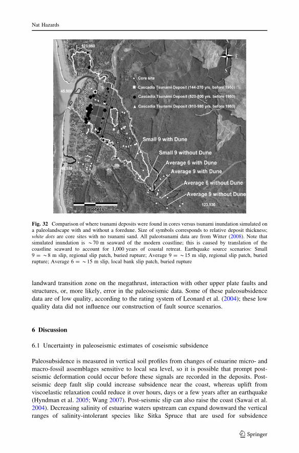
landward transition zone on the megathrust, interaction with other upper plate faults and
structures, or, more likely, error in the paleoseismic data. Some of these paleosubsidence
data are of low quality, according to the rating system of Leonard et al. (2004); these low
quality data did not influence our construction of fault source scenarios.
6 Discussion
6.1 Uncertainty in paleoseismic estimates of coseismic subsidence
Paleosubsidence is measured in vertical soil profiles from changes of estuarine micro- and
macro-fossil assemblages sensitive to local sea level, so it is possible that prompt post-
seismic deformation could occur before these signals are recorded in the deposits. Post-
seismic deep fault slip could increase subsidence near the coast, whereas uplift from
viscoelastic relaxation could reduce it over hours, days or a few years after an earthquake
(Hyndman et al. 2005; Wang 2007). Post-seismic slip can also raise the coast (Sawai et al.
2004). Decreasing salinity of estuarine waters upstream can expand downward the vertical
ranges of salinity-intolerant species like Sitka Spruce that are used for subsidence
Fig. 32 Comparison of where tsunami deposits were found in cores versus tsunami inundation simulated ona paleolandscape with and without a foredune. Size of symbols corresponds to relative deposit thickness;white dots are core sites with no tsunami sand. All paleotsunami data are from Witter (2008). Note thatsimulated inundation is *70 m seaward of the modern coastline; this is caused by translation of thecoastline seaward to account for 1,000 years of coastal retreat. Earthquake source scenarios: Small9 = *8 m slip, regional slip patch, buried rupture; Average 9 = *15 m slip, regional slip patch, buriedrupture; Average 6 = *15 m slip, local bank slip patch, buried rupture
Nat Hazards
123

estimates; this factor may be the principal reason much of the paleosubsidence data from
the Columbia River exceed our source scenarios.
6.2 Uncertainty in paleoseismic recurrence (fault slip)
The four recurrence intervals used to define small, average, large, and largest slip scenarios
were picked in 2007 from turbidite ages available at that time. While uncertainty inherent
in the dating techniques is on the order of ±100–300 years at 2r, new age data and
analysis became available during the course of the investigation, leading to mismatches
between 2007 and 2009 data. Changes were generally minor for all but the largest
recurrence intervals, which, as previously explained, were the most difficult to date (see
Fig. 33 Correspondence at the outer coast of scenario coseismic deformation to paleosubsidence data forthe AD 1700 Cascadia earthquake of Leonard et al. (2004) (diamonds with error bars) and Nelson et al.(2008) (open bars; one open arrow indicating that value is a minimum for the locality). Deformations shownas gray lines are from Cascadia earthquake sources S1–S12 of the TPSW (2006) investigation; black linesare sources of this investigation (labeled ‘‘DOGAMI models’’ in top charts). Note that many TPSWdeformations have subsidence larger than the AD 1700 data as do many of the ‘‘Largest’’ scenarios of thisinvestigation. B. = beach; R. = river; DOGAMI = Oregon Department of Geology and Mineral Industries
123

Priest et al. 2009 for detailed discussion). The largest mean recurrence in 2007 was
1,298 years (2r range of 1,110–1,440 years), leading to use of this interval for the largest
slip. This interval is still within the 2r root mean square error of the largest recurrence in
Table 1 for full-margin events (i.e., without event T5b), but must be viewed as a highly
conservative scenario.
Mismatches between turbidite size and the prior or following intervals indicate caution in
adopting individual intervals as a metric for the largest event. Because the correlation of
turbidite size to time between turbidites is only a modest one (Goldfinger et al. 2009; Priest
et al. 2009), strict adherence to these times is not warranted. Furthermore, evidence suggests
that smaller events use very little energy, and skew the interevent time values inappropriately.
For example, event T12 was preceded by *850 years (2r range of 584–1,115 years), and
followed by 700 years (2r range of 410–986 years), yet it was the smallest-mass turbidite of
those considered here (Table 1). The *1,550 year interval (2r range of 1,283–1,808 years)
between T13 and T11 represents *45 m of plate motion, yet only turbidite T12 occurred
during that period. We suspect that much of that strain was released in the earthquake that
caused one of the largest turbidites, T11, though the preceding and following times for T11
Fig. 34 Correspondence from Youngs Bay east along the Columbia River of scenario coseismicdeformations to paleosubsidence data of Leonard et al. (2004) for the AD 1700 Cascadia earthquake(diamonds with error bars). Deformations shown as gray lines are from Cascadia earthquake sourcesS1–S12 of the TPSW (2006) investigation; black lines are sources of this investigation
Nat Hazards
123

were not extraordinary. As previously discussed, we came to similar conclusions when
comparing simulated inundation to distribution of Cascadia tsunami deposits. The small-
volume turbidite, T2, provided a very short minimum interevent time (slip) that would be
inconsistent with observed tsunami deposits. We conclude that use of any turbidites as small
as or smaller than T2 for calculation of interseismic intervals likely causes underestimation of
slip. If this is the case, then we might ignore T12 in the T11–T13 interval and assign a
maximum interseismic time of 1,550 years rather than 1,300 years. Viewed in this context,
1,300 years is not overly conservative.
Our assumption that the coupling ratio is 1.0 for calculation of maximum slip from
recurrence data probably overestimates potential slip to some extent. McCaffrey (1997)
argues that the closest subduction zone analogues to Cascadia in terms of thermal regime
have a large component of aseismic slip (coupling ratio \1.0). He suggests that much of
the slip release at Cascadia could be in the form of ‘‘slow earthquakes’’ that would greatly
reduce seismic shaking. He explains the observation by Satake et al. (2003) that a large
Cascadia earthquake caused the AD 1700 tsunami by calling on slow earthquakes that can
produce significant tsunamis but little seismic shaking. Depending on how much slip is too
slow to be tsunamigenic, we could be overestimating tsunamigenic slip based on interevent
times.
6.3 Uncertainty in the local basin and bank slip patch sources
Wells et al. (2003) hypothesized that higher coseismic slip will be centered under forearc
sedimentary basins and used gravity lows as a proxies for these basins. In Oregon,
Nehalem Bank was predicted as one of these slip patches, but it is both a structural high
and a gravity low. This apparent contradiction is due to youthful development of the bank
from recently re-accreted materials from the local Columbia River source (Kulm et al.
1973). We modified our sources such that the bank is an area of low slip in our basin slip
patch source to be consistent with the basin model proposed by Wells et al. (2003).
Alternatively, if the gravity signature is important apart from being a basin proxy (Song
and Simons 2003), then our local slip patch model does not capture that possibility, one for
which there is no clear physical explanation.
6.4 Uncertainty in the fault dislocation model
The Wang and He (2008) fault dislocation model, as applied here, does not allow sig-
nificant slip near the deformation front owing to the velocity-strengthening assumption, but
there is some uncertainty about this assumption. According to Wang and He (2008) there is
speculation that, in the course of the evolution of pore fluid pressure distribution, parts of
the up-dip segment at some subduction zones may occasionally become moderately
velocity-weakening and, when triggered to slip, acquire tsunamigenic rupture speed (Seno
2002). Earthquakes characterized by this type of coseismic slip are ‘‘tsunami earthquakes’’
with relatively high slip near the deformation front, low felt shaking, and produce rela-
tively large tsunamis. While we cannot rule out these earthquakes on the Cascadia sub-
duction zone, the widespread occurrence of turbidites offshore (e.g., Goldfinger et al.
2003a, 2009) and liquefaction features onshore (Obermeier and Dickenson 2000) is con-
sistent with at least moderate coseismic ground motion over wide areas for the vast
majority of Cascadia events. Additional slow slip of the outer wedge remains a possibility.
There is also significant uncertainty about the down-dip extent of coseismic ruptures.
Some of this uncertainty is demonstrated by up to *25 km mismatch between the lateral
123

position of the modeled down-dip extent and the ‘‘stress line’’ (Fig. 8) that came about from
trials that matched modeled subsidence to paleosubsidence data of Leonard et al. (2004).
Szeliga et al. (2008) found from inversions of geodetic data that the preponderance of slow
slip events on Cascadia takes place down dip of the 25-km depth contour on the subducting
plate. Our modeled down-dip extent approximates the 25-km depth contour (Fig. 8), but
insufficient observation time has elapsed for these geodetic data to assess whether slip in the
lower part of the megathrust interface reduces plate convergence strain as fast as it accu-
mulates on the locked zone (Szeliga et al. 2008). More importantly, the geodetically inferred
down-dip limit of interseismic locking can be very different from the down-dip limit of
coseismic rupture because of the viscoelastic behavior of the system (Wang et al. 2003). In
view of the rather small differences in tsunamis generated by ±20 km in rupture width
(Fig. 25) uncertainty in rupture width is at best a second order concern.
6.5 Uncertainty in the hydrodynamic model
The hydrodynamic model, SELFE, passed all standard tsunami benchmark tests (Zhang
and Baptista 2008) and closely reproduced observed inundation and flow depths of the
1964 Alaska tsunami in Cannon Beach, thus we have considerable confidence in the code.
The model was run with zero friction, so it probably overestimates inundation somewhat,
although match of the simulated and observed inundation for the 1964 tsunami in devel-
oped areas indicates that the overestimate may be small where heavy vegetation is not
present. We can speculate that degree of overestimate probably depends on how far
inundation proceeds and how many obstacles the flow encounters. In low lying areas like
the Ecola Creek valley where closely spaced trees and other vegetation could slow tsu-
namis, the overestimate could be significant. The practical significance is that the minimum
coseismic slip of *14–15 m for inundation beyond paleotsunami deposits may be
somewhat larger than inferred here. A further practical result is that inundation at a
particular confidence limit is at a maximum for that limit. A full analysis of the friction
parameters relative to empirical observations was beyond the scope of this investigation.
6.6 Tsunamis from southern Cascadia earthquakes
In this investigation, we do not consider segment ruptures of the Cascadia subduction zone
in southern Oregon. Cannon Beach is north of inferred southern Oregon segment ruptures
(Goldfinger et al. 2008, 2009), and would not be expected to experience significant tsu-
namis from such events, given the directivity of tsunami energy away from the long axes of
seismic sources (Titov et al. 1999). One caveat on this expectation is the conclusion of
Myers (1999) that tsunami energy is more efficiently radiated north from southern segment
ruptures than south from northern ruptures on the Cascadia subduction zone.
6.7 Key observations
Lack of local historical observations of Cascadia tsunamis creates high uncertainty in esti-
mation of the hazard, but parametric analysis of geologically reasonable coseismic defor-
mations allows quantification of this uncertainty. Simulated Cascadia tsunami elevation and
inundation varied linearly with fault slip, thus understanding how much slip is reasonable is
critical. Paleoseismic estimates of earthquake recurrence were thus the key constraint on
tsunami hazard. Maximum runup for Cascadia tsunamis varied from 9 to 30 m, but tsunamis
Nat Hazards
123

approaching 30 m required*38 m of slip, an event that may have happened only once in the
last 10,000 years, according to interseismic intervals inferred from turbidite data. Minimum
slip of 14–15 m on the Cascadia subduction zone is needed to produce tsunamis large enough
to cover the three tsunami sands deposited over the last *1,000 years at Cannon Beach.
Arrival times of tsunami wave peaks varied little among the 25 Cascadia source scenarios
(26–34 min), but the time of first significant (3-m) rise of water elevation at the shoreline was
lower (10 min) for slip patches confined to submarine banks relative to regional slip patches
(17–23 min). Amplified uplift on a splay fault caused up to 31% increase in runup and up to a
20% increase in inundation, so accurate depiction of splay faults is also critical. Cascadia fault
rupture models that placed slip patches on a regional Cascadia locked zone or on local
submarine banks were most consistent with available geodetic, paleosubsidence, paleots-
unami, geological, and geophysical data. Cascadia sources with fault slip confined to forearc
basins or with slip skewed seaward from a symmetrical distribution (e.g., scenarios of TPSW
2006) were less consistent with these data.
Perhaps the most useful product of this work is providing confidence levels that Cas-
cadia inundation will not exceed certain elevations or mapped boundaries. For example,
the 99th percentile inundation line for Cascadia sources is at nearly twice the elevation of
the 90th percentile line in most areas of Cannon Beach.
Resources were inadequate to do a complete parametric analysis of all distant tsunami
sources, so we simulated only two maximum-considered events. The hydrodynamic sim-
ulation matched observed inundation from the largest historical distant tsunami, the 1964
Gulf of Alaska event, with open coastal runup of *6.5 m (maximum of 8.2 m). Open
coastal runup of *11 m (maximum of 12.4 m) from a hypothetical maximum-considered
Gulf of Alaska event was similar to the ‘‘preferred’’ Cascadia scenario (highest logic tree
weight) at *10 m (maximum of 12.2 m).
7 Conclusions and recommendations
This paper illustrates a useful technique for estimation of tsunami hazard posed by a local
subduction zone earthquake where considerable geological and geophysical data exist. We
demonstrate that differences in source geometry cause large differences in resulting tsu-
namis, underlining the critical importance of accurate, geologically reasonable tsunami
source characterization. Historical and prehistorical (paleotsunami) observations provided
ground truth checks of the approach. The chief parameters controlling Cascadia tsunami
size from most to least important are megathrust slip magnitude, enhanced uplift from a
splay fault, rupture extent, and distribution of slip. Twenty-five Cascadia earthquake
sources and resulting tsunami simulations adequately explored the variation of local tsu-
nami hazard to the Washington and northern Oregon coast. Ideally, tsunami hazard
assessments for this region would employ all 25 sources to produce percentile inundation
lines that express the confidence level (percentage) that a Cascadia tsunami will not exceed
each line. However, if simulation of all 25 sources is not possible, an adequate assessment
at other nearby sites may be accomplished with fewer sources drawn from this study (see
Priest et al. 2009, for digital source deformation data). The five sources that best represent
Cascadia source variability are
1. Scenario Average 9, regional Cascadia slip patch on a buried rupture, produces
minimum inundation consistent with the last three Cascadia tsunami deposits;
produces inundation encompassing *50% confidence limit.
123

2. Scenario Average 14, regional Cascadia slip patch on a splay fault, has highest logic
tree weight; produces inundation encompassing *70% confidence limit.
3. Scenario Large 14, regional Cascadia slip patch on a splay fault, produces inundation
encompassing *90% confidence limit.
4. Scenario Largest 14, regional Cascadia slip patch on a splay fault, produces inundation
encompassing *99% confidence limit.
5. Either the scenario Largest 1 (local bank slip patch) or Largest 2 (local basin slip
patch) scenario, whichever is the larger uplift, explores minimum tsunami arrival time.
If resources do not allow a complete parametric analysis of distant tsunamis, we rec-
ommend simulation of only one or two maximum-considered events:
1. Maximum-considered distant tsunami from the Gulf of Alaska (Source 3 of TPSW
2006) and
2. If local observational data are available, simulation of the tsunami from the 1964
Prince William Sound earthquake for ground truth check on the hydrodynamic
modeling approach.
If evacuation planning is the chief objective, only two simulations need be accom-
plished, scenario Largest 14 and the maximum-considered distant tsunami source (source 3
of TPSW 2006). These scenarios define tsunami evacuation zones for Cannon Beach (see
Cannon Beach evacuation map at http://www.oregongeology.org/pubs/tsubrochures/
CannonEvac.pdf).
This investigation is the first phase of a state of Oregon project aimed at tsunami hazard
assessment of the entire Oregon coast. The second phase is a similar detailed analysis of the
Bradley Lake-Bandon area of the southern Oregon coast where subduction zone geology is
significantly different and smaller Cascadia rupture lengths occur (e.g., Kelsey et al. 2005;
Goldfinger et al. 2008, 2009). The latter project is expected to be complete in 2010.
Acknowledgments This investigation was supported by National Oceanic and Atmospheric Adminis-tration (NOAA) Requisition Number NRMAH000-6-01035 through Oregon Department of Geology andMineral Industries (DOGAMI) Intergovernmental Agreement number 61110-09192006, and support fromthe City of Cannon Beach, the Cannon Beach Rural Fire Protection District, and the Seaside School Districtthrough Intergovernmental Agreement 41180-63006. The Pacific Marine Environmental Laboratory ofNOAA kindly provided earthquake source data for the two distant tsunami scenarios and cooperated at everystage of the investigation. Harvey Kelsey of Humboldt State University, Vasily Titov of NOAA and EricGeist of the US Geological Survey provided key reviews of an early draft. Brian Atwater of the USGSreviewed a later draft and offered key advice on paleosubsidence data. The authors acknowledge WesternGeco and the US Geological Survey for providing some of the seismic reflection data for the purpose of thisresearch. Angie Venturato of NOAA produced the initial compilation of topographic and bathymetric data.Charles Seaton of the OGI School of Science and Engineering, Oregon Health & Science Universityprovided key support with data reduction at all stages of the project. Ian Madin, Vicki McConnell and DonLewis of DOGAMI provided helpful review and advice. We thank local stakeholders for their wise counciland cooperation, particularly Al Aya and Cleve Rooper of the Cannon Beach Rural Fire Protection District,Richard Mays and Jay Raskin of the City of Cannon Beach, and Doug Dougherty, Superintendent of theSeaside School District.
References
Adam J, Klaeschen D, Kukowski N, Flueh E (2004) Upward delamination of Cascadia Basin sediment infillwith landward frontal accretion thrusting caused by rapid glacial age material flux. Tectonics23:TC3009
Adams J (1990) Paleoseismicity of the Cascadia subduction zone: evidence from turbidites off the Oregon-Washington margin. Tectonics 9:569–583
Nat Hazards
123

Allan JC, Priest GR (2001) Evaluation of coastal erosion hazard zones along the dune and bluff backedshorelines in Tillamook County, Oregon, Cascade Head to Cape Falcon, Preliminary Technical Reportto Tillamook County. Oregon Department of Geology Mineral Industries Open-File Report O-01-03
Ammon CJ, Ji C, Thio H-K, Robinson D, Ni S, Hjorleifsdottir V, Kanamori H, Lay T, Das S, Helmberger D,Ichinose G, Polet J, Wald D (2005) Rupture process of the 2004 Sumatra–Andaman Earthquake.Science 308:1133–1139
Atwater BF, Nelson AR, Clague JJ, Carver GA, Yamaguchi DK, Bobrowsky PT, Bourgeois J, Darienzo ME,Grant WC, Hemphill-Haley E, Kelsey HM, Jacoby GC, Nishenko SP, Palmer SP, Peterson CD,Reinhart MA (1995) Summary of coastal geologic evidence for past great earthquakes at the Cascadiasubduction zone. Earthq Spectra 11(1):1–18
Atwater BF, Tuttle MP, Schweig ES, Rubin CM, Yamaguchi DK, Hemphill-Haley E (2004) Earthquakerecurrence inferred from paleoseismology. In: Gillespie AR, Porter SC, Atwater BF (eds) The Qua-ternary period in the United States. Dev Quat Sci 1:331–348
Atwater BF, Musumi-Rokkaku S, Satake K, Tsuji Y, Ueda K, Yamaguchi DK (2005) The orphan tsunami of1700—Japanese clues to a parent earthquake in North America. US Geological Survey ProfessionalPaper 1707
Barrientos SE, Ward SN (1990) The 1960 Chile earthquake: inversion for slip distribution from surfacedeformation. Geophys J Int 103:589–598
Burgette R, Weldon RJ, Schmidt D (2007) A more accurate vertical velocity field for coastal Oregon revealsvariations in extent of locking on the Cascadia subduction zone. Eos Trans Am Geophys Union, vol 88(G52A-01)
Burgette R, Weldon RJ, Schmidt D (2009) Interseismic uplift rates for western Oregon and along-strikevariation in locking on the Cascadia subduction zone. J Geophys Res 114:B01408. doi:10.1029/2008JB005679
Chlieh M, Avouac J-P, Hjorleifsdottir V, Song T-RA, Ji C, Sieh K, Sladen A, Hebert H, Prawirodirdjo L,Bock Y, Galetzka J (2007) Coseismic slip and afterslip of the great (Mw 9.15) Sumatra–Andamanearthquake of 2004. Bull Seismol Soc Am 97(1):S152–S173
Cummins PR, Hori T, Kaneda Y (2001) Splay fault and megathrust earthquake slip in the Nankai Trough.Earth Planets Space 53(4):243–248
Dragert H, Hyndman RD (1995) Continuous GPS monitoring of elastic strain in the northern Cascadiasubduction zone. Geophys Res Lett 22:755–758
Fisher D, Mosher D, Austin JA, Gulick SPS, Masterlark T, Moran K (2007) Active deformation across theSumatran forearc over the December 2004 Mw 9.2 rupture. Geology 35:99–102
Fluck P, Hyndman RD, Wang K (1997) 3-D dislocation model for great earthquakes of the Cascadiasubduction zone. J Geophys Res 102:20539–20550
Freund LB, Barnett DM (1976) A two-dimensional analysis of surface deformation due to dip-slip faulting.Bull Seismol Soc Am 66:667–675
Global Centroid Moment Tensor Database (2007) http://www.globalcmt.org/CMTsearch.html. Accessed 2April 2007
Goldfinger C (1994) Active deformation of the Cascadia forearc: implications for great earthquake potentialin Oregon and Washington. Dissertation thesis, Oregon State University, Corvallis, OR
Goldfinger C, McNeill LC (2006) Sumatra and Cascadia: parallels explored. Eos Trans Am Geophys Union87:52
Goldfinger C, Mackay ME, Moore GF, Kulm LD, Yeats RS, Appelgate B (1992) Transverse structuraltrends along the Oregon convergent margin: implications for Cascadia earthquake potential and crustalrotations. Geology 20(2):141–144
Goldfinger C, Kulm LD, Yeats RS, Hummon C, Huftile GJ, Niem AR, Fox CG, McNeill LC (1996) Obliquestrike-slip faulting of the Cascadia submarine forearc: the Daisy Bank fault zone off central Oregon. In:Bebout GE, Scholl D, Kirby S, Platt JP (eds) Subduction top to bottom. Geophys Monogr 96:65–74
Goldfinger C, Kulm LD, Yeats RS, McNeill LC, Hummon C (1997) Oblique strike-slip faulting of thecentral Cascadia submarine forearc. J Geophys Res 102:8217–8243
Goldfinger C, Nelson CH et al (2003a) Deep-water turbidites as Holocene earthquake proxies: the Cascadiasubduction zone and northern San Andreas fault systems. Annali Geofisica 46(5):1169–1194
Goldfinger C, Nelson CH et al (2003b) Holocene earthquake records from the Cascadia subduction zone andnorthern San Andreas Fault based on precise dating of offshore turbidites. Ann Rev Earth Planet Sci31:555–577
Goldfinger C, Nelson CH, Morey-Ross A, Johnson JE, Baptista A, Zhang J, Wang K, Witter R, Priest G(2007) Interplay of structure and sediment supply may influence subduction zone rupture patches andpropagation. Eos Trans Am Geophys Union, Fall Meet Suppl vol 88 (T52A-07)
123

Goldfinger C, Grijalva K, Burgmann R, Morey A, Johnson JE, Nelson CH, Gutierrez-Pastor J, Ericsson A,Karabanov E, Chaytor JD, Patton J, Gracia E (2008) Late Holocene rupture of the northern SanAndreas Fault and possible stress linkage to the Cascadia subduction zone. Bull Seismol Soc Am98(2):861–889
Goldfinger C, Nelson CH, Morey A, Johnson JE, Gutierrez-Pastor J, Eriksson AT, Karabanov E, Patton J,Gracia E, Enkin R, Dallimore A, Dunhill G, Vallier T, The Shipboard Scientific Parties (2009)Turbidite event history: methods and implications for Holocene paleoseismicity of the Cascadiasubduction zone. US Geological Survey Professional Paper 1661-F
Hebenstreit GT, Murty TS (1989) Tsunami amplitudes from local earthquakes in the Pacific Northwestregion of North America, part 1—the outer coast. Mar Geodesy 13:101–146
Hyndman RD, Wang K (1995) The rupture zone of Cascadia great earthquakes from current deformationand the thermal regime. J Geophys Res 100:22133–22154
Hyndman RD, Leonard LJ, Currie CA (2005) Test of models for the Cascadia great earthquake rupture areausing coastal subsidence estimates for the 1700 earthquake. Final Report, US Geological SurveyNEHRP External Grant Award 04HQGR0088
Johnson J, Satake K, Holdahl S, Sauber J (1996) The 1964 Prince William Sound earthquake: joint inversionof tsunami and geodetic data. J Geophys Res 101(B1):523–532
Kelsey HM, Nelson AR, Hemphill-Haley E, Witter RC (2005) Tsunami history of an Oregon coastal lakereveals a 4600 yr record of great earthquakes on the Cascadia subduction zone. Geol Soc Am Bull117:1009–1032
Konca AO, Avouac JP, Sladen A, Meltzner AJ, Sieh K, Peng Fang P, Li Zhenhong Z, Galetzka J,Genrich J, Chlieh C, Natawidjaja DH, Bock Y, Fielding EJ, Ji C, Helmberger DV (2008) Partialrupture of a locked patch of the Sumatra megathrust during the 2007 earthquake sequence. Nature456:631–635
Kulm LD, Von Huene R, The Shipboard Scientific Party (1973) Initial reports of the Deep Sea DrillingProject, 18. Washington, DC, US Government Printing Office, pp 97–168
Lander JF, Lockridge PA, Kozuch MJ (1993) Tsunamis affecting the West Coast of the United States, 1806–1992. NGDC Key to Geophysical Records, Documentation no. 29
Leonard LJ, Hyndman RD, Mazzotti S (2004) Coseismic subsidence in the 1700 great Cascadia earthquake:coastal estimates versus elastic dislocation models. Geol Soc Am Bull 116:655–670
Mandal N, Chattopadhyay A, Bose S (1997) Imbricate thrust spacing: experimental and theoretical analyses.In: Sengupta S (ed) Evolution of geological structures in micro- to macro-scales, Chapter 8.1.Chapman and Hall, London
Mann DM, Snavely PD Jr (1984) Multichannel seismic-reflection profiles collected in 1977 in the easternPacific Ocean off of the Washington/Oregon coast. US Geological Survey Open-File Report 84-0005
McCaffrey R (1997) Influences of recurrence times and fault zone temperatures on the age-rate dependenceof subduction zone seismicity. J Geophys Res 102(B10):22839–22854
McCaffrey R, Long MD, Goldfinger C, Zwick PC, Nabelek JL, Johnson CK, Smith C (2000) Rotation andplate locking at the southern Cascadia subduction zone. Geophys Res Lett 27:3117–3120
McCaffrey R, Qamar A, King RW, Wells RW, Khazaradze G, Williams C, Stevens C, Vollick JJ, Zwick PC(2007) Fault locking, block rotation and crustal deformation in the Pacific Northwest. Geophys J Int169:1315–1340
McCrory PA, Blair JL, Oppenheimer DH, Walter SR (2004) Depth to the Juan de Fuca slab beneath theCascadia subduction margin—a 3-D model for sorting earthquakes. US Geological Survey Data SeriesDS-91. http://pubsusgsgov/ds/91/. Accessed 5 Sept 2006
McNeill LC, Piper KA, Goldfinger C, Kulm LD, Yeats RS (1997) Listric normal faulting on the Cascadiacontinental margin. J Geophys Res 102(B6):12123–12138
McNeill LC, Goldfinger C, Kulm LD, Yeats RS (2000) Tectonics of the Neogene Cascadia forearc basin:investigations of a deformed late Miocene unconformity. Geol Soc Am Bull 112(8):1209–1224
Mitchell CE, Vincent P, Weldon RJ II, Richards MA (1994) Present-day vertical deformation of theCascadia margin, Pacific northwest, USA. J Geophys Res 99:12257–12277
Mofjeld HO, Foreman MGG, Ruffman A (1997) West Coast tides during Cascadia subduction zone tsu-namis. Geophys Res Lett 24(17):2215–2218
Myers EP III, Baptista AM (2001) Analysis of factors influencing simulations of the 1993 Hokkaido Nansei-Oki and 1964 Alaska Tsunamis. Nat Hazards 23:1–28
Myers EP III (1999) Physical and numerical analysis of long wave modeling for tsunamis and tides.Dissertation thesis, Oregon Graduate Institute of Science & Technology, Hillsboro, OR
Nelson AR, Kelsey HM, Witter RC (2006) Great earthquakes of variable magnitude at the Cascadiasubduction zone. Quat Res 65:354–365
Nat Hazards
123

Nelson AR, Sawai Y, Jenningsc AE, Bradleya L, Gersonc L, Sherrod BL, Sabeane J, Horton BP (2008)Great-earthquake paleogeodesy and tsunamis of the past 2000 years at Alsea Bay, central Oregoncoast, USA. Quat Sci Rev 27:747–768
Ng MK-F, LeBlond PH, Murty TS (1990) Simulation of tsunamis from great earthquakes on the Cascadiasubduction zone. Science 250:1248–1251
Obermeier SF, Dickenson SE (2000) Liquefaction evidence for the strength of ground motions resultingfrom Late Holocene Cascadia subduction earthquakes, with emphasis on the event of 1700 AD. BullSeismol Soc Am 90(4):876–896
Okada Y (1985) Surface deformation due to shear and tensile faults in a half-space. Bull Seismol Soc Am75(4):1135–1154
Olmstead D (2003) Development in Oregon’s tsunami inundation zone: information guide for developersand local government. Oregon Department of Geology Mineral Industries Open-File Report O-03-05
Park JO, Tsuru T, Kodaira S, Cummins PR, Kaneda Y (2002) Splay fault branching along the Nankaisubduction zone. Science 297:1157–1160
Plafker G (1972) Alaskan earthquake of 1964 and Chilean earthquake of 1960: Implications for arc tec-tonics. J Geophys Res 77:901–925
Preuss J, Hebenstreit GT (1998) Integrated tsunami-hazard assessment for a coastal community, GraysHarbor, Washington. US Geological Survey Professional Paper 1560 vol 2, pp 517–536
Priest GR (1995) Explanation of mapping methods and use of the tsunami hazard maps of the Oregon coast.Oregon Department of Geology Mineral Industries Open-File Report O-95-67
Priest GR, Allan JC (2004) Evaluation of coastal erosion hazard zones along dune and bluff backedshorelines in Lincoln County, Oregon: Cascade Head to Seal Rock, Technical Report to LincolnCounty. Oregon Department of Geology Mineral Industries Open-File Report O-04-09
Priest GR, Myers E, Baptista A, Kamphaus RA, Peterson C (1997) Cascadia subduction zone tsunamis:hazard mapping at Yaquina Bay, Oregon. Oregon Department of Geology Mineral Industries Open-File Report O-97-34
Priest GR, Chawla A, Allan JC (2007) Tsunami hazard map of the Florence-Siuslaw River area, LaneCounty, Oregon. Oregon Department of Geology Mineral Industries IMS-25
Priest GR, Goldfinger C, Wang K, Witter RC, Zhang Y, Baptista AM (2009) Tsunami hazard assessment ofthe Northern Oregon coast: a multi-deterministic approach tested at Cannon Beach, Clatsop County,Oregon. Oregon Department of Geology Mineral Industries Special Paper 41
Rikitake T (1999) Probability of a great earthquake to recur in the Tokai district, Japan: reevaluation basedon newly-developed paleoseismology, plate tectonics, tsunami study, micro-seismicity and geodeticmeasurements. Earth Planets Space 51(3):147–157
Satake K, Shimazaki K, Tsuji Y, Ueda K (1996) Time and size of a giant earthquake in Cascadia inferredfrom Japanese tsunami records of January 1700. Nature 379:246–249
Satake K, Wang K, Atwater BF (2003) Fault slip and seismic moment of the 1700 Cascadia earthquakeinferred from Japanese tsunami descriptions. J Geophys Res 108:ESE7-1–ESE7-17
Sawai Y, Satake K, Kamataki T, Nasu H, Shishikura M, Atwater BF, Horton BP, Kelsey HM, Nagumo T,Yamaguchi M (2004) Transient uplift after a 17th-century earthquake along the Kuril subduction zone.Science 306:1918–1920
Schmidt D, Burgette R, Weldon R (2007) The distribution of interseismic locking on the central Cascadiasubduction zone inferred from coastal uplift rates in Oregon. Eos Trans Am Geophys Union vol 88(T52A-04)
Seno T (2002) Tsunami earthquake as transient phenomena. Geophys Res Lett 29(10):1419. doi:10029/2002GL014868
Song T-RA, Simons M (2003) Large trench-parallel gravity variations predict seismogenic behavior insubduction zones. Science 301:630–633
Szeliga W, Melbourne T, Santillan M, Miller M (2008) GPS constraints on 34 slow slip events within theCascadia subduction zone, 1997–2005. J Geophys Res 113:B04404. doi:10.1029/2007JB004948
Tadepalli S, Synolakis CE (1994) The run-up of N-waves on sloping beaches. Proc R Soc Lond A 445:99–112
Titov VV, Mofjeld HO, Gonzalez FI, Neuman JC (1999) Offshore forecasting of Hawaiian tsunamisgenerated in Alaskan-Aleutian subduction zone. NOAA Technical Memorandum ERL PMEL-114
Titov VV, Gonzalez FI, Mofjeld HO, Neuman JC (2001) Project SIFT (short term inundation forecasting fortsunamis). International tsunami symposium 2001 proceedings, vol 7-2, pp 715–721
Trehu AM, Braunmiller J, Nabelek JL (2008) Probable low-angle thrust earthquakes on the Juan de Fuca-North America plate boundary. Geology 36:127–130
123

Tsunami Pilot Study Working Group (2006) Seaside, Oregon tsunami pilot study—modernization of FEMAflood hazard maps. National Oceanic and Atmospheric Administration OAR Special Report, NOAA/OAR/PMEL, Seattle, WA
Walsh TJ, Caruthers CG, Heinitz AC, Myers EP III, Baptista AM, Erdakos GB, Kamphaus RA (2000)Tsunami hazard map of the southern Washington coast; modeled tsunami inundation from a Cascadiasubduction zone earthquake. Wash Division of Geology and Earth Resources Geologic Map GM-49
Wang K (2007) Elastic and viscoelastic models of crustal deformation in subduction earthquake cycles. In:Dixon T, Moore JC (eds) The seismogenic zone of subduction thrust faults. Columbia University Press,New York, pp 540–575
Wang K, He J (1999) Mechanics of low-stress forearcs: Nankai and Cascadia. J Geophys Res 104(B7):15191–15205
Wang K, He J (2008) Effects of frictional behaviour and geometry of subduction fault on coseismic seafloordeformation. Bull Seismol Soc Am 98(2):571–579
Wang K, Hu Y (2006) Accretionary prisms in subduction earthquake cycles: the theory of dynamic Cou-lomb wedge. J Geophys Res 111:B06410. doi:10.1029/2005JB004094
Wang K, Wells R, Mazzotti S, Hyndman RD, Sagiya T (2003) A revised dislocation model of interseismicdeformation of the Cascadia subduction zone. J Geophys Res 108(B1):2026. doi:10.1029/2001JB001227
Wells RE, Blakely RJ, Sugiyama Y, Scholl DW, Dinterman PA (2003) Basin-centered asperities in greatsubduction zone earthquakes: a link between slip, subsidence, and subduction erosion. J Geophys Res108(B10):2507. doi:101029/2002JB002072
Werner KS, Graven EP, Berkman TA, Parker MJ (1991) Direction of maximum horizontal compression inwestern Oregon determined by borehole breakouts. Tectonics 10(5):948–958
Whitmore PM (1993) Expected tsunami amplitudes and currents along the North American coast forCascadia subduction zone earthquakes. Nat Hazards 8:59–73
Witter RC (2008) Prehistoric Cascadia tsunami inundation and runup at Cannon Beach, Oregon. OregonDepartment of Geology Mineral Industries technical report to the Cannon Beach Rural Fire ProtectionDistrict. Oregon Department of Geology Mineral Industries Open-File Report O-08-12
Zhang Y, Baptista AM (2008) An efficient and robust tsunami model on unstructured grids part I: inundationbenchmarks. Pure Appl Geophys 165(11–12):2229–2248. doi:101007/s00024-008-0424-7
Nat Hazards
123