CONDITIONAL SIMULATION – WHICH METHOD FOR MINING?

Jacqui Coombes1, Gordon Thomas2, Ian Glacken3 and Viv Snowden4

1 Consultant Geostatistician, Snowden M.I.C., 87 Colin St, West Perth, Australia, 6005.2 Manager Technology, Snowden M.I.C., 87 Colin St, West Perth, Australia, 6005.3 Manager Resources Division, Snowden M.I.C., 87 Colin St, West Perth, Australia, 6005.4 Director, Snowden M.I.C., 87 Colin St, West Perth, Australia, 6005.

1.0 Introduction

There is an increasing awareness of the sensitivities in conditional simulation to sample and assay quality,

geological interpretations and structural controls, and variogram parameters such as the nugget effect. A

wide range of algorithms and applications has been proposed, presented and discussed (ISGSM 1999, held in

Perth, Australia, is the most recent international meeting to focus solely on conditional simulation and its

applications for the mining industry).

Conditional simulation is now being used more regularly in the mining industry to communicate uncertainty

and to enhance understanding of risk. The potential upside or downside must be meaningful for descriptions

of risk to be of value in mine design or decision making. Either overstated or understated risk will mislead,

resulting in sub-optimal designs or bad decisions. An inappropriate description of risk may be costly or

result in a lost opportunity. It is recognised that good simulation requires as much care, if not more care,

than estimation.

The interpretation of geological controls, grade distribution, mineralisation continuity and data spacing,

together with the conditional simulation algorithm selected, all have an influence on the modelled variability.

This study investigates the impact on the description of risk and the subsequent mining decisions, depending

on which conditional simulation algorithm is used to communicate uncertainty within a number of geological

settings and sampling scenarios.

2.0 Study method

Three case studies are presented here using data sets from real projects. Each data set provides a different

perspective for risk analysis in the mining industry. The first data set is a bench of densely-sampled grade

control data. The second data set represents regularly-drilled, but widely spaced exploration drilling for an

orebody that is to be mined by open pit methods. The third data set comprises relatively sparse underground

fan drilling for an orebody at the pre-production phase.

Each data set was fully analysed to provide appropriate simulation parameters. All three scenarios were then

subject to conditional simulation using sequential Gaussian (SGS) and sequential Indicator (SIS) techniques.

These two techniques are arguably still the most common simulation algorithms in use in the mining

industry. Full descriptions of the algorithms and implementation aspects are given in Deutsch and Journel

(1998). Simulations were carried out using as many common parameters as possible for the respective SGS

and SIS runs, including the random number seed, the search details, and the combination of original

conditioning data and previously-simulated nodes. The simulation results were comprehensively validated,

and were then compared using grade-tonnage curves. A grade-tonnage curve is generated by averaging

nodes into block grades and accumulating the respective tonnages above a series of cut-off grades. The

average grades are then plotted against the tonnages at each cut-off. One grade-tonnage curve is produced

per realisation. Grade-tonnage curves are a useful tool for comparing the relative values of models and

different realisations across simulation algorithms.

3.0 Case study 1 – grade control data

The first data set comprises a single bench of gold grade control data sampled on an 8 m x 8 m grid over four

distinct geological domains, each of which require unique estimation and simulation parameters. Parameters

for each domain are based on the quantitative data as well as the qualitative geological understanding of the

deposit.

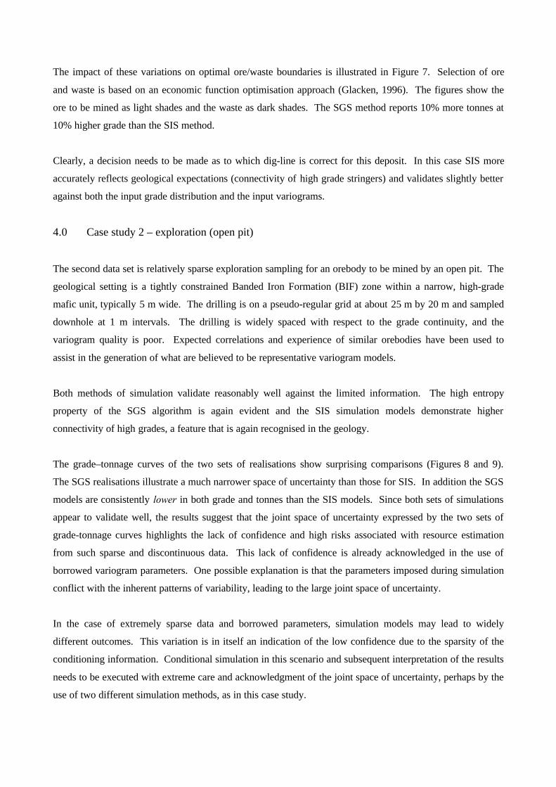
Histograms, statistics and variograms for all 50 realisations for each simulation algorithm were validated

against the conditioning information. Q-Q plots comparing quantiles of the original composited grade control

data with the point simulation results are presented for the SGS models in Figure 1 and for the SIS models in

Figure 2.

SGS is known to be a maximum entropy algorithm in that it maximises the disconnectedness of high and low

grade values. This property of the SGS realisations is evident when compared with a typical SIS realisation

from the grade control data in plan view (Figures 3 and 4). The SIS model is able to reproduce the

geological anisotropy, which is present as a consequence of the existence of high grade stringers in this

deposit.

The SGS models report consistently more tonnes at higher grades than SIS for all cut-offs (SGS grade-

tonnage curves are closer to the top of the graph in Figure 5). The SIS best case scenario tends to equate to

the worst case SGS scenario (Figure 6). The SIS models show a slightly wider space of uncertainty,

resulting in wider confidence intervals and more inherent risk when expected grades or tonnes above specific

cut-off grades are reported.

The impact of these variations on optimal ore/waste boundaries is illustrated in Figure 7. Selection of ore

and waste is based on an economic function optimisation approach (Glacken, 1996). The figures show the

ore to be mined as light shades and the waste as dark shades. The SGS method reports 10% more tonnes at

10% higher grade than the SIS method.

Clearly, a decision needs to be made as to which dig-line is correct for this deposit. In this case SIS more

accurately reflects geological expectations (connectivity of high grade stringers) and validates slightly better

against both the input grade distribution and the input variograms.

4.0 Case study 2 – exploration (open pit)

The second data set is relatively sparse exploration sampling for an orebody to be mined by an open pit. The

geological setting is a tightly constrained Banded Iron Formation (BIF) zone within a narrow, high-grade

mafic unit, typically 5 m wide. The drilling is on a pseudo-regular grid at about 25 m by 20 m and sampled

downhole at 1 m intervals. The drilling is widely spaced with respect to the grade continuity, and the

variogram quality is poor. Expected correlations and experience of similar orebodies have been used to

assist in the generation of what are believed to be representative variogram models.

Both methods of simulation validate reasonably well against the limited information. The high entropy

property of the SGS algorithm is again evident and the SIS simulation models demonstrate higher

connectivity of high grades, a feature that is again recognised in the geology.

The grade–tonnage curves of the two sets of realisations show surprising comparisons (Figures 8 and 9).

The SGS realisations illustrate a much narrower space of uncertainty than those for SIS. In addition the SGS

models are consistently lower in both grade and tonnes than the SIS models. Since both sets of simulations

appear to validate well, the results suggest that the joint space of uncertainty expressed by the two sets of

grade-tonnage curves highlights the lack of confidence and high risks associated with resource estimation

from such sparse and discontinuous data. This lack of confidence is already acknowledged in the use of

borrowed variogram parameters. One possible explanation is that the parameters imposed during simulation

conflict with the inherent patterns of variability, leading to the large joint space of uncertainty.

In the case of extremely sparse data and borrowed parameters, simulation models may lead to widely

different outcomes. This variation is in itself an indication of the low confidence due to the sparsity of the

conditioning information. Conditional simulation in this scenario and subsequent interpretation of the results

needs to be executed with extreme care and acknowledgment of the joint space of uncertainty, perhaps by the

use of two different simulation methods, as in this case study.

5.0 Case study 3 – exploration (underground)

The third data set is taken from an underground mining operation. There is a complex combination of

lithological and structural controls on mineralisation, and four domains have been defined on this basis.

Each domain has its own continuity characteristics, which have been inferred from the data in and around the

simulation area. The conditioning data come from relatively sparse yet pseudo-regular fan drilling off

underground drives. Figure 12 shows a three-dimensional view of the simulation area and the relevant

conditioning data.

The characteristic high entropy of the SGS method is again evident in Figure 10. The SIS realisations have a

smaller range in simulated grade values (Figures 11 and 12).

The more appropriate method in this case appears to be SGS, since the high entropy reflects the lack of

connectivity evident and well-known from existing mining in this geological setting. In addition, some

domains show extreme positive skewness and very high grade outliers which are difficult to represent using

indicator thresholds and upper tail modelling functions.

The two methods again demonstrate very different descriptions of uncertainty. This time the SGS models

report significantly more tonnes at significantly higher grades for a given cut-off than the SIS models (Figure

12).

The impact of these differences for mine design is significant. The realisations for the best and worst case

tonnage scenarios and the best and worst case grade scenarios for each simulation technique were evaluated

using a stope optimisation procedure. This approach generates mineable underground stope shapes that

maximise the net present value of the project (Thomas and Earl, 1999). The stope outlines in Figures 13 and

14 highlight a 50% to 60% difference in stope volume for a 70% difference in metal between the

optimisations based on the two sets of simulations. Larger, more profitable stopes are defined using SGS,

which is deemed to be more appropriate for this setting. The more conservative SIS models would have led

to a considerable understatement of the reserves and hence the potential value of the project.

6.0 Discussion

Sensitivity to simulation methods has been shown by these examples to depend on one or more of the

following:

• DATA COVERAGE: Simulation models tend to be data-driven. When there is sufficient data, most

algorithms produce similar results. When the conditioning data are sparse, there is less data-charging of

the simulations, and models are much more sensitive to the way variogram parameters are used by each

algorithm.

• DIFFERENCES IN CONTROLLING PARAMETERS: The major differences in the controlling

parameters of the two methods presented here are the variogram definitions and the data

transformations. The SIS method has more detailed variogram definition that allows particular high or

low-grade characteristics to be incorporated into the simulation, in addition to the modelling of different

directions and amounts of continuity at different thresholds. The single variogram required by the SGS

method inherently overstates the shorter ranges of continuity for the extreme grades.

• ENTROPY: Geological environments which exhibit disconnected grades, such as some laterite or

oxidised deposits, stockwork or brecciated mineralisation, have genuine high entropy. Low entropy is

more characteristic of deposits which exhibit continuous lodes or structures, for example vein or shear-

zone hosted deposits.

Conditional simulation provides the practitioner with a useful tool to communicate uncertainty and risk to the

project decision-makers. An understanding of the geological ‘texture’ of each deposit will assist

practitioners in the mining industry to select the most appropriate conditional simulation technique and

parameters for each geological environment.

Acknowledgments

This paper summarises detailed ongoing investigations at Snowden that would not have been possible

without the dedication to quality by directors, the enthusiasm of the resource evaluation division, and the

assistance of the mining division. In particular, Steve Potter and Allan Earl gave their time and ideas.

References

Deutsch, C V, and Journel, A G, 1998. GSLIB Geostatistical software and users guide, Oxford University

Press, New York, 369p.

Glacken, I M, 1996. Change of support and use of economic parameters in block selection, in Geostatistics

Wollongong ’96 (Eds: Baafi E Y, and Schofield, N A) pp 811-821 (Kluwer, The Netherlands, 1997).

Thomas, G S, and Earl, A, 1999. The application of second-generation stope optimisation tools in

underground cut-off grade analysis, in Strategic Mine Planning – proceedings of ‘Optimising with

Whittle – 1999’, Whittle Programming, Victoria, pp175-180.

Figure 1: Q-Q plots between SGS models and input data (the grade control data)

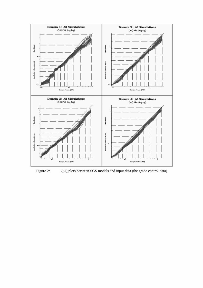
Figure 2: Q-Q plots between SGS models and input data (the grade control data)

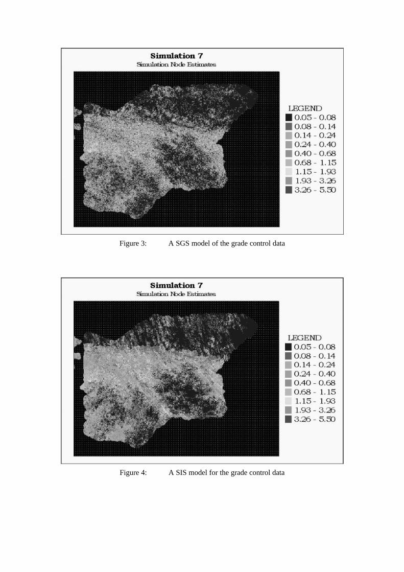
Figure 3: A SGS model of the grade control data

Figure 4: A SIS model for the grade control data

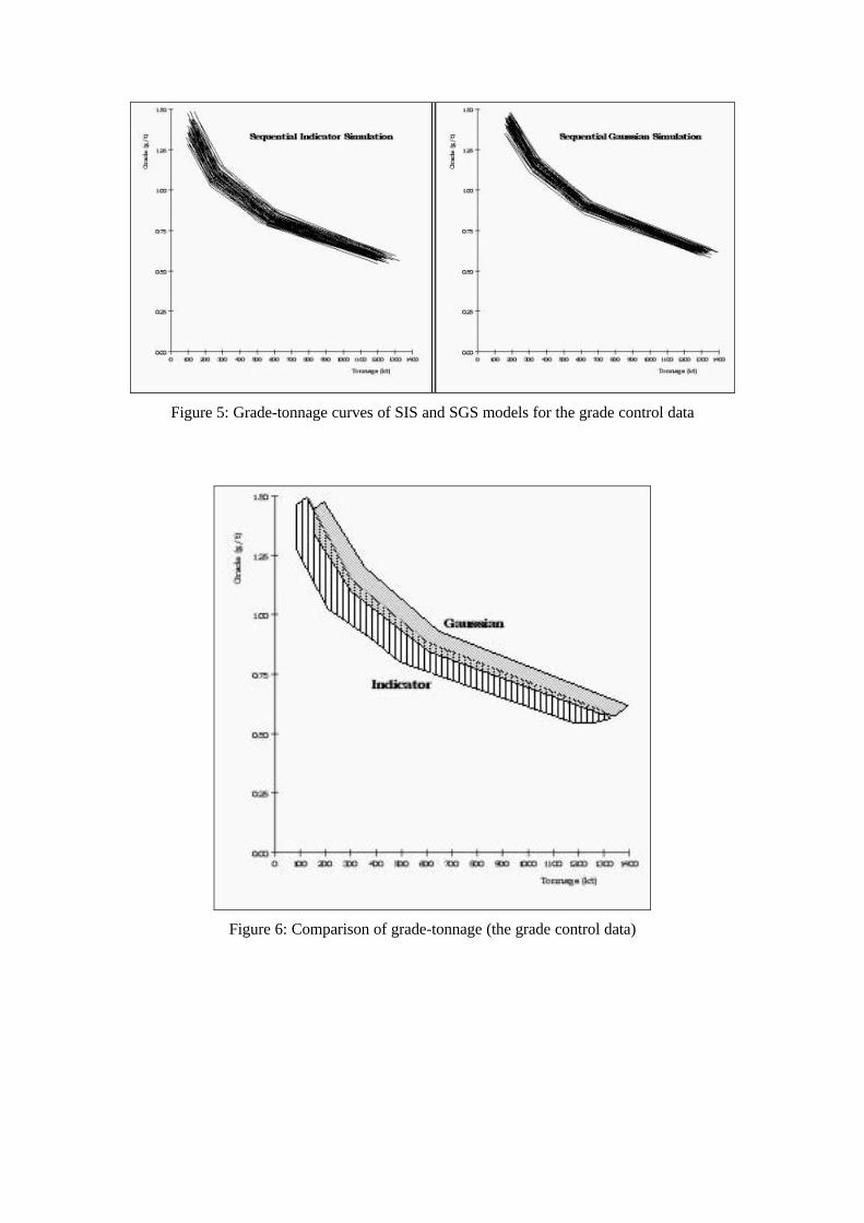
Figure 5: Grade-tonnage curves of SIS and SGS models for the grade control data

Figure 6: Comparison of grade-tonnage (the grade control data)

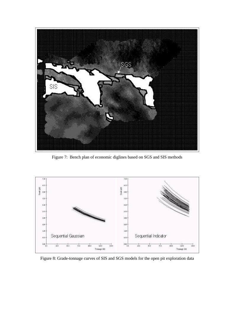
Figure 7: Bench plan of economic diglines based on SGS and SIS methods

Figure 8: Grade-tonnage curves of SIS and SGS models for the open pit exploration data

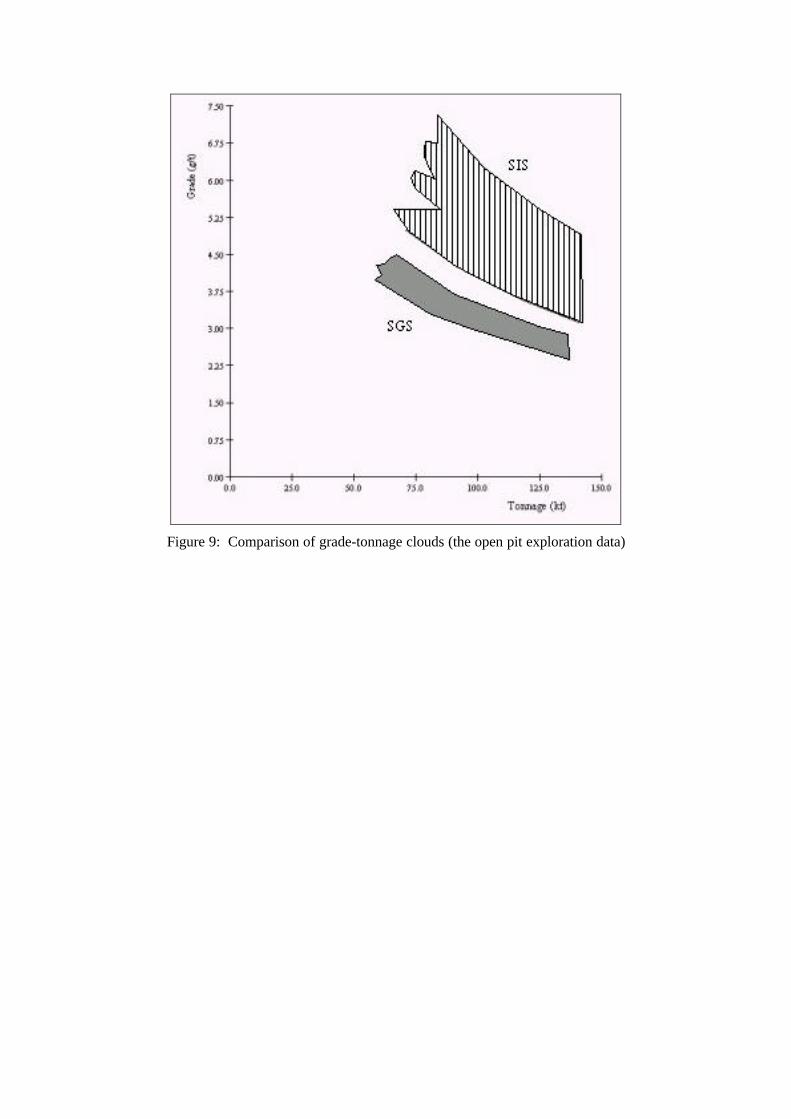
Figure 9: Comparison of grade-tonnage clouds (the open pit exploration data)

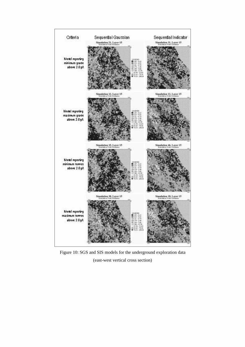
Figure 10: SGS and SIS models for the underground exploration data

(east-west vertical cross section)

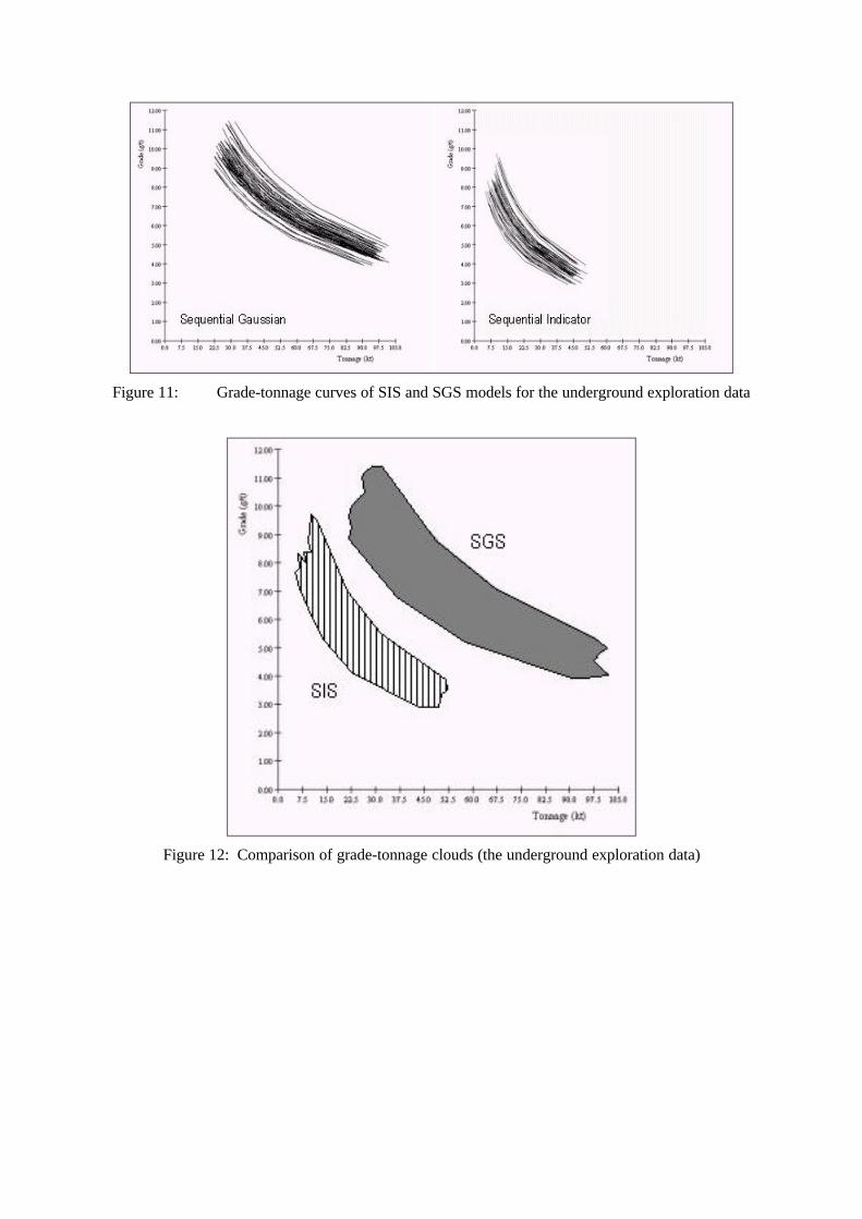
Figure 11: Grade-tonnage curves of SIS and SGS models for the underground exploration data

Figure 12: Comparison of grade-tonnage clouds (the underground exploration data)

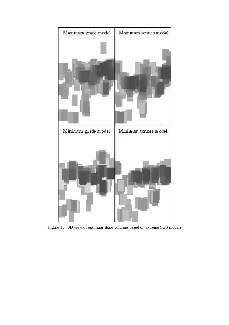
Figure 13: 3D view of optimum stope volumes based on extreme SGS models

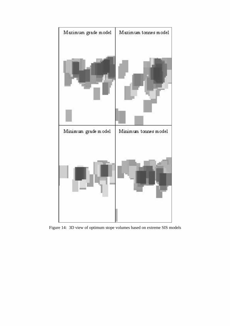
Figure 14: 3D view of optimum stope volumes based on extreme SIS models