Embed Size (px)
Citation preview
J. Phys. I FFance 7 (1997) 395-421 MARCH 1997, PAGE 395
Configurational Diffusionon a Locally Connected Correlated
Energy Landscape; Application to Finite,Random Heteropolymers
Jin Wang, Steven S. Plotkin and Peter G. Wolynes (*)
School of Chemical Sciences, University of Illinois, Urbana, IL 61801, USA
(Received 2 September J996, revised 22 November 1996, accepted 27 November 1996)
PACS.05.40.+j Fluctuation phenomena, random processes, and Brownian motion
PACS.05.70.Ln Nonequilibrium thermodynamics, irreversible processesPACS.05.90.+m Other topics in statistical physics and thermodynamics
Abstract. We study the time scale for diffusionon a correlated energy landscape using
models based on the generalized random energy model (GREM) studied earlier in the context
of spin glasses (Derrida B. and Gardner E., J. Phys. C lo (1986) 2253) with kinetically local
connections. The escape barrier and mean escape time are significantly reduced from the un-
correlated landscape (REM) values. Results for the mean escape time from a kinetic trap are
obtained for two models approximating random heteropolymers in different regimes, with linear
and bi-linear approximations to the configurational entropy versus similarity q with a given state.
In both cases, a correlated landscape results in a shorter escape time from a meta-stable state
than in the uncorrelated model (Bryngelson J-D. and Wolynes P.G., J. Phys. Chem. 93 (1989)6902). Results are compared to simulations of the diffusion constant for 27-mers. In general,there is a second transition temperature above the thermodynamic glass temperature, at and
above which kinetics becomes non-activated. In the special case of an entropy linear in q, there
is no escape barrier for a model preserving ultrametricity. However, in real heteropolymers a
barrier can result from the breaking of ultrarnetricity, as seen in our non-ultrarnetric model. The
distribution of escape times for a model preserving microscopic ultrametricity is also obtained,and found to reduce to the uncorrelated landscape in well-defined limits.
1. Introduction
The study of biomolecular dynamics in general and protein folding in particular has inspired
a good deal of study of the dynamics of disordered systems [Ii. Statistically defined energy
landscapes naturally emerge in biouiolecular physics because of the heteropolymeric complexityof a biomolecule's sequence. Many questions about the energy landscapes and dynamics of
biomolecules resemble the issues in the theory of ergodicity breaking in glasses and spin glasses
[2j but the mesoscopic scale of protein molecules means that hopping between globally distinct
minima, which in the thermodynamic limit would be strictly inaccessible, must be taken into
account, and may indeed dominate the experimental behavior iii. Starting with the work of
Bryngelson and Wolynes [3j the connection of the dynamics on statistical energy landscapes
and folding has been exploited both qualitatively to understand the perplexing complexity -of
(*) Author for correspondence (e-mail: wolynestlaries.scs.uiuc.edu)
@ Les (ditions de Physique 1997

396 JOURNAL DE PHYSIQUE I N°3
folding kinetics experiments and quantitatively in interpreting simulations [4,5j and developingprediction algorithms [6j. Foldable proteins contain an energetic bias towards a folded state
which is likely due to selection by natural evolution. On the other hand, as in typical mean
field spin glasses, there are many uncorrelated states which can act as kinetic traps, at least
transiently. Dynamics in the glassy phase for these systems has been studied using random
energy models [7,8j. The escape from these traps determines the effective diffusion coefficient
for flow of the ensemble of protein structures towards the folded state needed to give fast folding
on biologically relevant timescales. This general picture has been confirmed semiquantitatively
through the use of lattice uiodels of minimally frustrated heteropolymers [9,10j. The originalBW analysis [3j assumed that the rugged parts of the energy landscape could be modeled in the
most extreme form as a completely random landscape described by the random energy model
of Derrida [iii. Superimposed on this was the bias due to minimal frustration. The random
energy model belongs to a general class of disordered systems which lack special symmetries(e.g. time inversion symmetry in the Sherrington-Kirkpatrick model of a spin glass), and
having a discrete juuip in the order parameter q(x) describing the replica symmetry breaking,such as that seen in Potts glasses [12j. Other aspects of the low energy states are universal,such as the statistics of their non-self-averaging processes below the transition, and some of this
universality may carry over to the dynamics. The "first order" glass transition seen in random
heteropolymers (RHPS) by replica methods [13j puts these systems in the saute universalityclass as the REM as far as issues of ergodicity breaking are concerned.
While the random energy model, being in the right universality class, describes in a renoruial-
ized sense the nature of a random heteropolymer (RHP) landscape, for a quantitative theory(see for example [14j), it is certainly relevant to take into account the correlations in the land-
scape which are inherent in the polymeric nature of the problem. Recently Plotkin, Wang and
Wolynes have shown how the thermodynamics of glassy trapping [lsj and folding [16j can be
treated in this way. The thermodynamic glass transition temperatures are not much modified
in many cases, although the nature of the replica syuimetry breaking can change as a function
of the density. While the relevant transition temperatures are well determined by the random
energy model estimates, it was shown that the configurational entropy relevant to the nuuiber
of basins of attraction was significantly modified. In the original BW analysis, the Levinthal
paradox [17j arising from the consideration of the search time through possible conformational
states on a flat energy landscape was shown to be connected on a globally rough landscapewith the difficulties of escape from the traps on the random energy surface. Since the configu-rational entropy of the basins is changed in the correlated model, it is relevant to ask whether
siuiilar modifications occur when the kinetics are examined. In this paper we discuss the ki-
netics of escape from traps on a correlated energy landscape for two uiodels approximatingrandom heteropolyuiers (RHP). The first (hereafter referred to as the REM strata model, RS
model, orRSM) considers strata of states at a given similarity to a specified state, which are
uncorrelated to each other, but indeed correlated in energy to the specific state. In the second
model (hereafter the ultrametric model),an ultrametric hierarchy is imposed on all of the states
(equilibrium or not), the statistics of which are analyzed in the context of the generalized ran-
doui energy model (GREM) [18]. This uiicroscopic ultrametrieity is somewhat different than
the conventional thermodynamic ultrarnetricity used to describe equilibrium states in mean
field spin-glasses. The regions of validity for both of these models as deteruiined by the accu-
racy of their description of the true organization of states of a random heteropolymer are an
important issue. We analyze the dynamics for both models to obtain the average escape time
front a metastable trap. In calculating this diffusion time, linear and bi-linear approximations
to the configurational entropy as afunction of similarity Sc(q)
are employed [lsj. These simpleforms are chosen primarily for their illustrative value;
more complex forms suchas those used
N°3 DIFFUSION ON A CORRELATED ENERGY LANDSCAPE 397
In ( ( )
o
25~
~
~
~o ~
~
~
15 ~
~
~
lo
5~
0
11.2x

398 JOURNAL DE PHYSIQUE I N°3
We should also mention that the approach used in this paper, though arrived at in the
context of finite heteropolymers, is applicable as an approximation to any system describable
by a locally connected, correlated energy landscape.We organize this paper as follows: in Section 2, we review the description of the correlations
in the landscape that are required to model the heteropolymer, and obtain the free energy
relative to a given state. Free energy functions are obtained in two approximations, which
in the following sections are used to calculate escape barriers from basins of attraction. In
Section 3, we analyze the ground states and glass transition temperatures in the two models
described in Section 2. In Section 4, we study the kinetics of escape processes for a small
random heteropolymer (RHP) using a linear approximation of entropy as a function of specific
contacts, which can be applied to lattice model 27-mers often used to mimic the protein folding
process. In Section 5, we calculate the mean escape time from a basin of attraction for largeRHP'S using a piece-wise linear approximation to the entropy.
2. Correlated Free Energy Landscapes
In this section, we review the description of the energy statistics of a random heteropolymer(RHP) by a correlated energy landscape, highlighting those quantities used in the kinetic
analysis.For an RHP, each pair of interacting monomers mn has an interaction energy em
n
that can be
taken to be a Gaussian random variable. The contact Hamiltonian 7i for a given configurationis given by:
7~"
~6mnamn j2.i)
m<n
where amn =I when there is a contact made between monouiers mn in the chain, and
amn =0 otherwise. Here contact uieans that the two monomers mn are within a small distance
(contact radius) of each other. We assume as in lattice models that there is an additional partof the Hamiltonian which keeps the chain connected, and represents hard constraints, I.e. all
connected configurations which are allowed have the same energy at least as far as this partof the Hamiltonian is concerned. This is used for lattice models, and is likely a good approx-
imation for real proteins. In addition we assume the model contains hard excluded volume
forces, which again do not bias different allowed states. Both chain connectivity and excluded
volume contribute to the entropy, i-e- in the GREM approach we can separate the energeticand entropic issues, taking chain connectivity and excluded volume into account through the
counting of states of a lattice chain as a function of imposed constraints~ S(q) (see Eq. (2.5)).There are potentially interesting purely dynauiical effects connected with chain connectivityand excluded volume, however these are likely to be small for real, finite size proteins because
so much of the protein actually lies on the surface.
Because of the small number of nearest neighbors for realistic lattice models of proteins, manyinvestigations have shown the move set in the configurational search does not greatly alter the
result, and the problem of self avoidance is not a primary one [9j. However the dynamical glasstemperature TA described later in this paper is expected to increase as a result of hard-core
interactions. Indeed the hard core fluid shows a transition to activated behavior that depends
on density alone [21j.Since the total energy of the polymer is a sum of many random variables (contact energies),
it is approximately a Gaussian random variable with probability distribution
1 j~2~~~~
(27r~hE2)1/2~~~~ 2~hE2~' ~~'~~
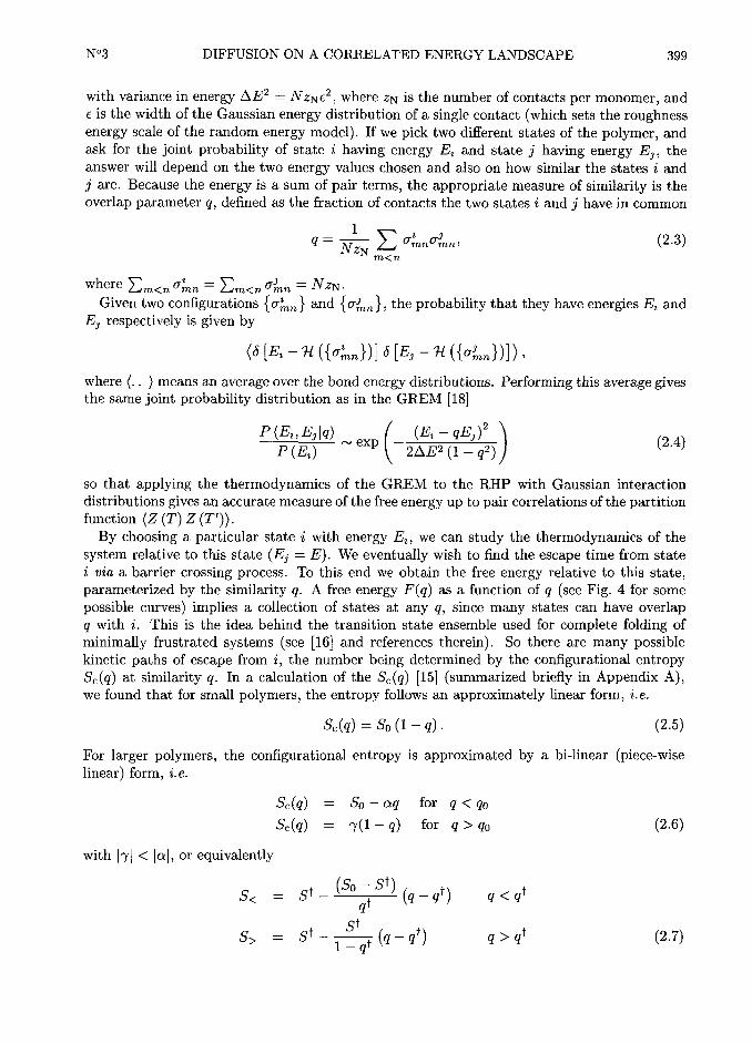
N°3 DIFFUSION ON A CORRELATED ENERGY LANDSCAPE 399
with variance in energy ~hE~=
NzNe~, where zN is the number of contacts per monouier, and
e is the width of the Gaussian energy distribution of a single contact (which sets the roughness
energy scale of the random energy uiodel). Ifwe pick two different states of the polynier, and
ask for the joint probability of state I having energy Ei and state j having energy Ej, the
answer will depend on the two energy values chosen and also on how siniilar the states I and
j are. Because the energy is a sum of pair terms, the appropriate measure of similarity is the
overlap parameter q, defined as the fraction of contacts the two states I and j have in common
~ NzN(~ °~~°~"' ~~'~~
where £~~~ a[~=
£~~~ a[~=
NzN.
Given two configurations (a[~ and (a[~ ), the probability that they have energies Ei and
Ej respectively is given by
(~ ilG ~i ii°uni)1~ i~J ~ ii°ini)i i'
where (. means an average over the bond energy distributions. Performing this average givesthe same joint probability distribution as in the GREM [18j
so that applying the thermodynamics of the GREM to the RHP with Gaussian interaction
distributions gives an accurate measure of the free energy up to pair correlations of the partitionfunction (Z (T) Z (T')).
By choosing a particular state I with energy Ei, we can study the thermodynamics of the
system relative to this state (Ej=
E). We eventually wish to find the escape time from state
I via a barrier crossing process. To this end we obtain the free energy relative to this state,parameterized by the similarity q. A free energy F(q) as a function of q (see Fig. 4 for some
possible curves) implies a collection of states at any q, since many states can have overlap
q with I. This is the idea behind the transition state ensemble used for couiplete folding of
minimally frustrated systems (see [16j and references therein). So there are many possiblekinetic paths of escape from I, the number being determined by the configurational entropy
Sc(q) at similarity q. In a calculation of the Sc(q) [lsj (summarized briefly in Appendix A),
we found that for small polymers, the entropy follows an approximately linear form, I.e.
sc(q)=
so (i q) (2.5)
For larger polymers, the configurational entropy is approximated by a bi-linear (piece-wiselinear) form, I-e-
Sc(q)=
So aq for q < qo
Sc(Q)"
'f(l Q) for q > qo (2.6)
with j~tj < )a), or equivalently
S<=
St ~~° ~~~(q qt q < qts/
S>=
St (q qt) q > qt (2.7)

400 JOURNAL DE PHYSIQUE I N°3
with St < So (I qf). We will use either of these notations depending on which one is more
advantageous in elucidating the results. Here go " q~ is the approximate crossover point where
the entropic behavior changes from bond formation to sequence melting [15] (see Appendix A).The energies of the states at q are distributed according to equation (2.4), so that the
microcanonical entropy is given by [25j
S(E, q, Ei) Q inexp
[Sc(q)]~
)j(j~~~ (2.8)
In this model there is no explicit overlap q' between states in the stratum at q, so that their
correlations with each other are not considered. The mean and width of the Gaussian distribu-
tion of energies for the states at q are explicitly q dependent due to their correlations with state
I, but in writing (2.8) we assume the relative fluctuations in n(E, q, Ei)= exp S(E, q, Ei) are
negligible, and n(E, q, E;) may be replaced by its average in the argument of the log (hence the
REM stratum model). This assumption is still reasonable when the number of states is large,but for smaller n(E, q, E~), it becomes important to investigate the distribution P in (E, q, E~)),
or at least moments beyond the first, e.g. in (Ei, q, E,)n(E2, Q, Ei)). Another point to mention
regarding (2.8) is that the description allows for the existence of "non-ultrametric" states hav-
ing less overlap with each other than they do with state I. This description can be said to be
accurate when uncorrelated states (with q12 =0 for states I and 2) predominate the number
distribution.
Proceeding within the REM strata model, we use the thermodynamic condition I IT=
05(E, q, E,) /0E to obtain the thermal energy and the thermal entropy [26]
E (q, T)=
qE~ ~)~ (l q~)
S (q, T)=
Sc(q) f~)( (I q~) (2.9)
from which the free energy of the band of states having overlap q with a given one can now be
written as~
Frs (q, Tl=
qEi Tsclql$ Ii q~) for T > Tc iq)
,
12.io)
where TG IQ) is given in equation (3.3). A free energy of this form was used to describe the
barrier in the folding transition [16j.The free energy obtained this way has in it the a prioTi assertion that there exists a state I
with energy Ei, which induces or designs the aspect of minimal frustration into the heteropoly-
mer. This, coupled with the fact that there can exist states with overlaps < q at each stratum
(non-ultrarnetric states), allows there to be states with lower energy than the REM groundstate E(s
=2So/~E2. This comes about because the ground state of the collection of
states having overlap q with I (E;=
E(~) is actually lower than E(~, due to the fact that the
correlated average of the distribution approaches E(~ faster than its width decreases due to
the REM stratum approximation. Because of this the barrier comes from deep states that are
correlated to I, but only weakly correlated to each other. Clearly the barrier in this case must
be interpreted as escape from a basin of attraction rather than a specific state. The problem of
minimizing the number of these states which are correlated but distinct from a designed state
is related to the problem of negative design. This effect of a correlated landscape was recentlyinvestigated in the context of optimized Hamiltonian approaches to structure prediction [27j.
For strata of highly similar states, it becomes increasingly likely that states in this band
arecorrelated to each other as well. In this regime, an ultrarnetric structure is a better
N°3 DIFFUSION ON A CORRELATED ENERGY LANDSCAPE 401
approximation to the organization of states of the heteropolymer. To this end we approximatethe free energy of the heteropolymer using the GREM hierarchy, which attributes contributions
to the energies of states on each branch of the ultrametric tree (see Ref. [18j and AppendixB). This model has a well-defined ground state energy, and we expect that the escape barriers,which in the RSM came from ultrametricity-breaking of meta-stable states, will be significantlymodified.
Appendix B contains calculations of: I) the distribution of escape times from a metastable
state at temperature T, 2) The distribution of free energy functions relative to a state I with
energy E~, both calculated in the context of the GREM, with an ultrametric organization of
states. The most probable form of the free energy as a function of q obtained there is
Fu(q, T)=
qE~ TSC(q)~~~
ii q) T > T(. (2.ll)
3. Ground States and Glass TeTnperatures
Below Tg, the kinetics is non-self averaging in that the rate of escape from a kinetic trap dependsnot just on its energy but differs from one trap to another. More elaborate tools need to be
developed in order to account for these non-self-averaging effects, which have applicationsto both molecqlar evolution and combinatorial synthesis. However we can make significantheadway by investigating the energies at the boundaries of statistical distributions of states,and the temperatures at which the system is frozen into these energies.
The ground state of the system is the energy at which the number of states
n(E)= exp (So P (E) m O II), where So is essentially the total number of states and PIE) is
given by equation (2.2):
E(s=
~@@. (3.I)
The system reaches the negative root of (3.I) at temperature T$=
~hE2 / (2So).Asserting the existence of a state I with energy Ej modifies the ground state energies.
For the RS model, the ground state in each stratum q is the energy where the exponentof (2.8)
=0,
EGS (q)=
qE~ ~ ~/2~hE2 II q2) Sc (q) (3.2)
which the system reaches at the q dependent glass temperature
~(3.3)(1 Q~) /~E
TG (q)" 2Sc (q)
For illustration, we approximate the configurational entropy as a linear function of con-
straint q, Sc(q)=
So(I q) Ian accurate approximation for small polymers), and assume
a designed ground state I with Ei=
E(s. The RS model predicts that the designed state
freezes first at v§Tj, and then a gradual freezing oicurs outward from the state I at Tjr'~a~=
Ill + q) ~hE2 / (2So) to which the system is frozen into energy E[]~~~(q)=
Ecs IQ + (I q)@@), until a ground state at q =
0 of E(s is frozen in at T(. The free energy at T( then
has a minimum at q Q 0.48 of Q I.llE(s and maxima at q =0 and q =
I of E[s.In an ultrametric model we can somewhat more rigorously investigate the freezing of pairs
of states with overlap q. Let two states aand b have energies Ea
=#< + #[ and Eb
=4< + #§
(as in Fig. 5 with #[=
#[ and #>=
#§). The log number of pairs with overlap q is
SpAiRs=
So + Sc(q). The ground state energy of #< at q, for two states having energies Ea
402 JOURNAL DE PHYSIQUE I N°3
and Eb, is the value of fi< where the log number of pairs
~ ~~ ~~~'~°'~~~ ~° ~ ~~ ~~~ 2~E2 ~~ ~ ~~i -~~~ ~~~l -~ ~~
vanishes. This gives
#(S=
~ ~~~ ~ ~~~~
~~~[2 (1 q~) (So + Sc (q) ~hE~ (E( 2qEaEb + El)] ~~~ (3.4)
1+ q+~
For a, b two ground states and a linear Sc(q), #(~ in (3.4) is frozen into its most probable value
(see Eq. (B.I))#(S (q)
=
qE(s (3.5)
at a temperature given by
0 In Qq ii<, Ea, Eb~ 04< jjs
or
~~~/~
~~. (~.~)°
An analogous calculation gives #)S=
ii q) E(~ at T£>=
~hE2 / (2So). So for an ultra-
metric model with a linear Sc(q), the freezing is q independent and equal to Tj,as would be
the case from a direct calculation in the GREM model [18j. The q-independent free energy for
T < T( is equal to E(s,so there are no states with lower energy than E[s. This will have
consequences for the kinetic escape barrier above T(, discussed in the next section.
4. Barriers and Escape Times for STnall PolyTners
In this section we calculate the mean escape time (T (T)) from a basin of attraction for a
small RHP, I, e. the average time required for the RHP to reconfigure to unrelated states by an
activated transition out of the basin of attraction. The inverse of this quantity is approximatelyequal to the diffusion constant on a rugged but correlated landscape.
For small polymers such as those describable by 27-mer lattice models, Plotkin, Wang,and Wolynes [lsj have shown that the configurational entropy crudely approximates a linear
function of constraint q (2.5). The mapping to lattice models should apply to significantlylarger proteins than the sequence length of the corresponding lattice model, depending on the
amount of secondary structure present [4].For an ultrametric model, it is simple to see that for a purely linear configurational entropy
there are no escape barriers above the thermodynamic glass temperature; barriers only appearbelow TG when the system is in the glass phase. The free energy (2.ll) is a linear function of
q with slope~£ j~2
~~° ~2T
~ ~
Now the largest escape barriers would occur when Ei happens to be a ground state, E~=
E(s.Letting T
=XT( where
x > I, this slope becomescc
(-2 + x + I /x), which is > 0 for all x > I
(all T > T[). Then the maximum of the free energy F is at the state itself (q=
I) and escape
is always a downhill diffusive process, with no activation barrier.

N°3 DIFFUSION ON A CORRELATED ENERGY LANDSCAPE 403
The situation is significantly different when the free energy is better approximated by REM
strata cf. Eq. (2,10)). For the purpose of obtaining escape times, we have set fl(Q)=
0 and
~hE2 (Q)=
~hE~ to simplify the calculation. We first note that because of the gradual onset of
freezing (see comments after Eq. (3.3)) starting at viT( down to T[, The free energy (2.10)is split into three temperature regimes:
T >V§T( F=Fm(q,E~,T)=qEj-TSO(I-q)-~~~(l-q~)
~o ~ ~ ~/~o F
=Fm lq, Ei, T) q < qG IT)
~ ~ F=
Ff IQ, Ei)=
qE~ Ii q) ~/2so~E2 ii + q) q > qc jTj
T <T( F=EGS=-fi~(q+(I-q)fi) (4.I)
where qG (T)=
(2SoT~/~hE~) I is the q value at temperature T where the frozen and
unfrozen "melted") free energy meet, I.e. the inverse of TG (q) (Eq. (3.3) with a linear Sc(q)).We seek the diffusion constant on the rough landscape of an RHP, approximated as
D(T)m
II jr (T)), by calculating the mean escape time jr (T)) at temperature T:
IT IT))= /(~~ dEiP lEi, TIT lE~, T) 14.2)
where P (E~, T) is the thermal distribution of energies at temperature T (see Eq. (B.6)), and
r(Ei,T) is defined below. The structure of the free energy in this model is such that there
exists a free energy minimum at a value of q e ql between q =0 and q =
I. The barrier to
escape from a given state (q=
I) to unrelated states (q=
0) is then just F(q=
0) F (ql).The escape time from a metastable state of energy E~ is essentially a Boltzmann factor of the
activation energy, times the number of ways to cross the barrier:
r (E~, T)= To exp (~ ~~ ~'~~ ~ ~~~'~'~~ l(4.3)
~
where for proteins To is on the order of micro seconds [24j. The largest contributions to jr IT)in (4.2) come from low energy states that have a barrier to escape. Higher energies that have
no barrier (downhill) have escape times Gt To
For purposes of calculation, we scale the temperature and energy to be in units of the REM
glass temperature and REM ground state:
T=
xT( XII
E=
vEis=
-y@W o I v I I 14.41
First note that there are typically no macroscopic barriers above viT(. The argument is as
follows: for typical thermal energies E~=
-~hE~ IT, the high temperature free energy (4.I)
is ccj-x I/x) + q ix 2/x) + q~ lx. There is no macroscopic barrier when the free energy
minimum 0F/0q=
0 occurs at ql=
0 or x =
vi. So above T=
viT(, kinetics is typically
non-activated.
A more detailed calculation in Appendix C using equation (4.2) achieves the same result, plus
the result that precisely at T=
v§Tj, the mean escape time scales as a power law in system
size ((r (v§T()+~
tJ (N~/~)). We mention again that in calculating the mean escape time,
404 JOURNAL DE PHYSIQUE I N°3
the integral over the region having an activation barrier dominates, and this region determines
the limits of the integral.For temperatures Tj < T <
v§T( where the system is partially frozen, the free energy (4.I)is split into two regimes: melted below qG lx)
=
x~ I and frozen above qG lx). Even within this
temperaturb range the calculation of the barrier and corresponding escape time must be splitagain into two temperature regions. The higher temperature region is defined by qG lx) > qliv
=I), which means that the minimum of the free energy is always in the melted region (since
ql iv)= x (2y x) /2 < ql II )), and the barrier is always calculated from Fm in equation (4.I).
Then the form of the expression for the escape time is identical to that above v§T(, but
the expressions in the exponent are now > 0, resulting in barriers that are now exponentiallylarge below v§T(. The crossover temperature x#T(
occurs when qG (x#)=
ql (y=
I, x#)or
x#=
(I + vi) /3. Below this temperature of Q 1.22 T(, there are energies where the escape
barrier must be calculated between the frozen minimum Ff (q =ql), and the melted maximum
Fm (q=
0). Expressions for the escape time in this temperature regime are split into two terms,
one contribution from high energies and onefrom low energies. As the temperature approaches
T( the mean escape time becomes
IT lTt)I=
j exP1°.225 x So) 14.5)
and the activation energy (energetic barrier) to jump from trap to trap is
~hF (T()=
~hE (T() a 0.l126 )E(s (4.6)
The escape time here is significantly smaller than in the REM, where (r (T()~~
= To exp So,although in both cases the escape barrier scales exponentially with system ~size N. For a
27-mer, (r (T())m 2 x 10~To, whereas (7 (T())~~~ m 10~~ro. A correlated landscape is
smoother, which results in a reduced search time. A consequence of this is that the number
TF/TG, which characterizes the degree of minimal frustration in a heteropolymer, does not
need to be so large for natural proteins as would appear from previous estimates based on the
REM. The escape barrier at T( for a correlated landscape is also smaller than in the REM
(~hEr~m=
T]So=
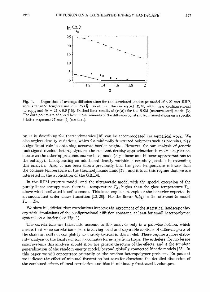
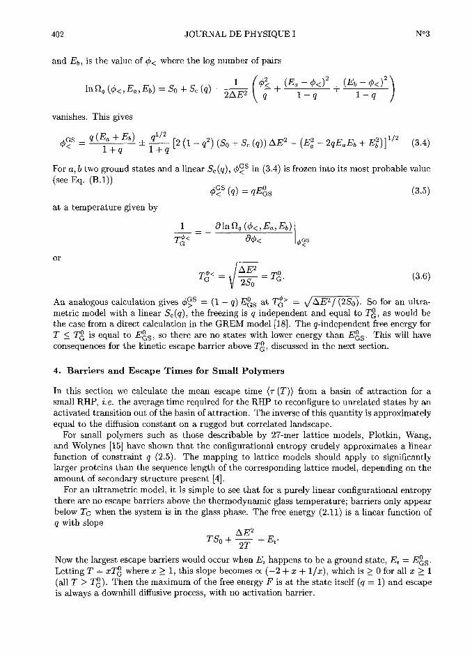
EGS/2).Figure 1 shows the log of the average diffusion time in units of To versus reduced temperature
x =
TIT(, using the parameter So appropriate fora collapsed 27-mer (So
=0.9 x 27). For the
correlated landscape the results of the calculation of Appendix C can be summarized as
To for v§TG< T
To CTG ~~ (§i + I) TG T(2fi$ T
~~~ ~~°T T2
(~ (j~)) ~ (~ j~ /j~ 3j~2 ~j~2+ ~~ l exp So
4 @ j)for TG < T < v§TG
2 (T /TG) T 4T~
2~k lc l) ~~~ ~~° ~~~ ~~ ~°~ ~ ~ ~~
~(4.7)
where TG %T(
=~hE2 / (2So), and c and gi are defined in Appendix C and are numerically
given by c Gt 1.477 and gi H 1.l13. We mention again that we neglect the coupling of polymerdensity with temperature, which can play a significant role. Also plotted in Figure I are
N°3 DIFFUSION ON A CORRELATED ENERGY LANDSCAPE 405
the results from the uncorrelated random energy landscape [3j:
~~ ~~~~~~~To exp
So2() j) ~ OT]j
for TG < T < 2TG '
~~'~~
G
To exp So for T < TG
and the results from simulations on the 27-mer [5j measuring the diffusion constant for a
specific 3-letter sequence II ID is plotted here, where D=
~hQ2 /room m I/room is the diffusion
constant in Q-space). Our theory does not estimate the number To in the simulations, which
depends on the details of the move set. Hence the values of the simulation data are normalized
so that at high temperatures the measufied correlation time coincides with To, the barrier-less
escape time. Notice that the escape time on the correlated landscape is much lower than
the uncorrelated result. In addition there is a temperature TA above which kinetics is non-
activated, again differing from the REM. Escape times calculated for the correlated model bythe analytic theory underestimate the escape times obtained in lattice simulations, but are
much closer to the simulated values than the simple REM results.
Notice again that the diffusion time drops to To at v§T(, where the dynamics is no longeractivated. Thus the correlated energy model possesses a transition which the REM does not,
froma high temperature regime with essentially no escape barriers to a low temperature regime
with escape barriers. This kind of behaviour with two characteristic temperatures (Tg and TA)is expected for the Potts glass and some of the more sophisticated models of the random
heteropolymer [12, 20j. The behavior in the correlated energy model considered here is similar,but the transition is not sharp for finite N. There are always some activated transitions from
traps.
For studying the special case of diffusion in a minimally frustrated polymer, we let Q rep-
resent the overlap with the native state, and q represent overlap among states with a given Q(there
are still many conformational states with a given overlap Q with respect to the native
state). In other words, folding progresses along the native order parameter by a typicallyactivated diffusional rate R(Q), which is evaluated by finding the escape time of meta-stable
states at each stratum Q. In each stratum, the energy distribution of states is given by
P(E~)m exp (E~ E (Q))~ /2~hE2 IQ)
,
and the configurational entropy is S(Q). In gen-
eral, states must have energies higher than E)~=
E(Q) ~/2~hE2(Q)S(Q) and lower than
E)+=
fi + ~/2~hE2(Q)S(Q), where the statistical numbers are macroscopic.
To a first approximation, the folding time of a minimally frustrated heteropolymer can then
be estimated as
~°~~ " i~~~
~~~ ~~~ ~~~~ ~~'~~
where ~hF=
F(Q) F(Qunfoid) is the thermodynamic folding free energy barrier, andr
IQ) is
the escape (diffusion) time in a particular stratum of similarity Q to the ground state. It is this
quantity T(Q) which is calculated below. The REM estimate for the escape time is given by
equation (4.8). The calculations in the remainder of this paper improve on these estimates of
the escape time (the exponentially large prefactor to the folding time due to transient trapping
in Eq. (4.9)), by taking into account correlations in the energy landscape. The time r(Q)is related to the diffusion constant D in the Kramers theory of folding [5] by r(Q)
m I ID,
406 JOURNAL DE PHYSIQUE I N°3
to within a constant of order one determined by the mean squared change ofthe order parameterin a single escape event.
5. Barriers and Escape TiTnes for Larger HeteropolyTners
As mentioned in Section 2, the configurational entropy for larger polymers can be approximatedby a bilinear form [lsj (cf. Eqs. (2.6, 2.7)). We can proceed with this form of the entropy to
find the average diffusion time at temperature T for larger heteropolymers. Here the effects of
the form of the configurational entropy on the kinetic glass temperature can be readily seen,and in the appropriate limit the REl/I result can be re-obtained.
5.I. DiffusioN AMONG ULTRAMETRICALLY ORGANIzED STATES. The analysis is similar
to that in the previous section with the simplification that the free energy is linear in q, however
it is a piece-wise function of q. Using the scaling in equation (4.4), the piece-wise free energyrelative to state I with energy E~ is
~@j I jl Stj x jj
~ 2~ x~~ x~
So qt ~Y ~~~
fit St I I St~~
~
2~soli-qtl~~i~~ i~soli-qtl~~~~ ~~~' ~~'~~
This piece-wise linear free energy has no escape barrier from I at q =I when the slope of F>
is > 0. This occurs naturally at high energies or y < yA (x) where
~~ ~~~ 2So
~~-qtj ~ + lx ~~'~~
Equation (5.2) sets an upper limit to the energies contributing to the escape time.
Using the typical (thermal) energies at temperature T in (5.2), I.e. E~=
-~hE2 IT or
yA =I /fA, gives a crude estimate of the temperature flA above which escape barriers vanish
and kinetics is non-activated. While this estimate will turn out not to give very accurate
numerical values of the kinetic transition temperature TA, it is useful in describing the trends
in TA in the limits of linear configurational entropy (St /So=
I qt) and a cratered, REM-likelandscape (St,qt
~ 0). The results will be numerically crude because energies deeper than
the thermal energy contribute most to the escape time.
Solving (5.2) for fA gives
xi=
[=
fiG
or
y~
~ 2St(5.3)
Note IA~ cc when St
~ 0. Losing all the entropy at qtmeans that the system must
jump out of a large energetic barrier before it gains entropy to compensate (but note in this
approximation q' needs not ~ 0). This means that effectivelywe have a "cratered" free energy
landscape, on which kinetics is always activated at all temperatures. This limit reproduces the
result of the REM analysis, which also has such a pock-marked landscape because states are
uncorrelated, and there is no "knowledge" of the existence of a low energy state until that
state is reached.
N°3 DIFFUSION ON A CORRELATED ENERGY LANDSCAPE 407
When St /So=
I qt, Sc(q) is a purely linear function of q. For this special case flA=
T]as obtained in the last section, and there are no activation barriers until T < T(. Energeticlosses are always exactly balanced by entropic gains. A more accurate calculation of TA will
be given below.
Equation (5.3) is precisely the higher temperature scale of the two step GREM for a givenbilinear Sc(q). [18j Following Derrida's analysis of the GREM, a bilinear Sc(q) with St /So <
I qt, has only one thermodynamic glass temperature T(=
~hE2/(2So) above which the
system is in its unfrozen phase. The above analysis gives significance to the higher temperatureTA, which did not enter into the thermodynamic analyses.
The barrier height (over T) to escape from a state I at temperature XT( is
~hF 2 (1- qt) St (I qt)I ~°
x
~ So x2~~'~~
which vanishes for high energy states Ei > yAE(~, and is largest at T(x =
I and y =I)
when it is given by
/~F-
fitIi Qt
II15.51
Note that (5.5) equals the REM barrier of T] So=
E(~ /2 when St, qt ~ 0 (again,a cratered
landscape), and that when St /So=
I qt la linear Sc(q)), ~hF=
0, as obtained in the last
section.
The average escape time from equation (4.2) is then
i~ (xii- ro lo exp -so
II+
I IIx
[<~,dv exP So 2Y ~~
~~~ ~i
=
jexp s~
2 3qt + ~t 2 ~~
~~ So
~~~ ~(2 qt
~j
~~~~° ~
~~~i
~~t~~ ~~
The integral is dominated by the ground state energy y =I, I.e. the lowest energies contribute
most to the average escape time. Using a large N approximation for the error functions, the
mean escape (diffusion) time for a long RHP with ultrametric states is given by
Tofor TA < T
~fi 12q~)
jII
~~~~~~~~~P~0(2(2~~~)~/~(2~~~)~ ~~
~~~~G~~~~~
~A ii ~ti -~exP So Ii ~t Ill for T < TG
IS-?)
where TG eT(. TA, the temperature above which kinetics is typically non-activated, is given
by the vanishing of the exponent in IS.?)
y~~ m
~~ ~~f + (~ qf) (i qf
~~ l. (5_8)1 + (~~/~0) ~0

408 JOURNAL DE PHYSIQUE I N°3
in iii
50 REM
40 ~,'30 3'
~'
2° 2,~~',10 ~ ',
~ ',0 '
2 3 4 5
X
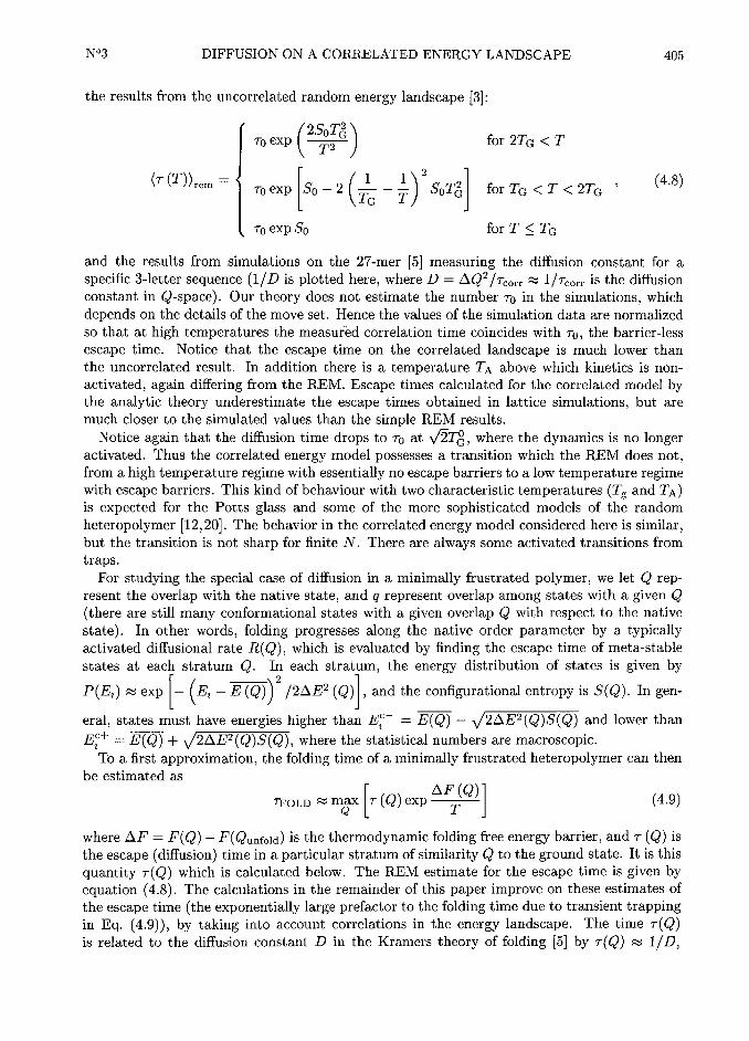
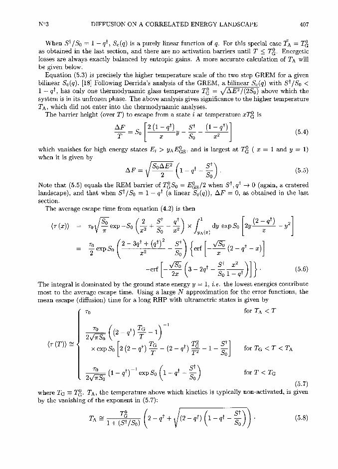
Fig. 2. The escape time in the correlated model approaches the REM result in the limit of a cratered
landscape. Plotted here is equation (5.6) with the parameters of a typical 64-mer So G£ 0.9 x 64,Si
=0A x 640 and qi
=0.290, where a =
1, 2/3,1/3, 0. The a =0 result essentially coincides with
the REM result, with the small deviation coming from the prefactor.
The point iA given earlier (fA in Eq. (5.3)) is a point of inflection for the curve marking the
onset of the decay of activation barriers for a finite system. However the escape time at these
temperatures is still large. More accurate values of TA can be obtained from (5.8), which givegood agreement to the temperature where jr (x)) becomes Gt To It can be seen from (5.8) that
when the configurational entropy is purely linear (St /So=
1- qt), TA ~T(,
as obtained in the
previous section. When Sc(q) is linear (St /So=
I qt), the escape times are non-exponentialand scale as +~
N~~/2.
When St, qf ~ 0 the free energy landscape is highly cratered, and the escape time becomes
(~ (j~0 $~0
~SQ (~ g)G ~ ~~
which reproduces the REM scaling with entropy. In other words, even though the landscape is
correlated, the escape time agrees with the REM because the polymer must entirely reconfigure
to escape a kinetic trap there is little entropic gain until many bonds are broken. To obtain
the behavior of TA in the limit ofa cratered landscape, we must use equation (5.6) rather
than IS.?) since xA is large and thus the error functions are small but not insignificant. For
St, qt ~ 0, the value of y maximizing the integrand in (5.7) is ymax =2 lx (the energies with
largest contribution become the statistically most probable energies for a cratered landscape),from which (5.7) becomes
jr (x))~~~~+~ exp (~)
,
(5.10)x
from which we can see that kinetics is still activated as in the Ferry law, with exponentiallylarge barriers, until x ~ cc or TA ~ cc.
The mean escape time from a basin of attraction, as given by equations (5.6, 5.7) is signifi-cantly less than the REM. In Figure 2, results are shown using equation (5.6) for the 64-mer
with S(~ Gt 0.4 x 64 and q(~ Gt 0.29. Results are also plotted as the landscape goes over to the
REM (cratered) one, by taking St=
oS(~ and qt=
oq(~ and letting a ~ 0.
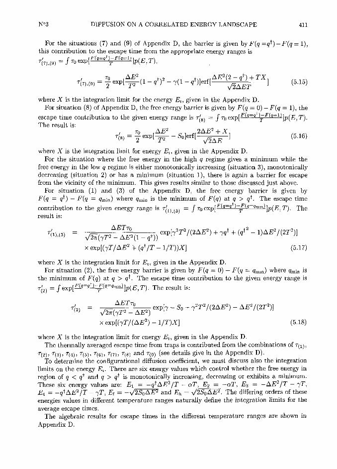
The log of the mean escape time, using parameters appropriate for the 64-mer and 125-mer
in equation (5.6), are shown in Figures 3a and 3b. The steepest descents approximation (5.7)

N°3 DIFFUSION ON A CORRELATED ENERGY LANDSCAPE 409
l~ ~~in I
TI
T~~~
30
8 25
6-,
20 ''",,,
~
'"',,15
"',,,",,
10"',
'
2 ',,,~
",,~
0"" ""
l 1.2 IA 1.6 1.8 2 1.2 IA 1.6 1.8 2
al X b) X
Fig. 3. al Logarithm of average diffusion (escape) time for the correlated landscape model of a 64
mer RHP versus reduced temperature x =
TIT(. A bi-linear approximation to the configurationalentropy is used, with total entropy So * 0.9 x 64. Solid line: (T ix)) for the ultrametric model.
Dashed line: (T ix)) for the REM stratum approximation. (The parameters used in the bilinear
entropy formulae (2.6, 2.7)are o =
64 x 1.55, 1= 64 x 0.56, orSi
=0.4 x 64 and qi
=0.29.) b)
Average escape time from a basin for a correlated landscape imitating a 125-mer. The curves are as
in the 64-mer case.(The parameters used in the bilinear entropy formulae (2.6, 2.7) are a =
125 x 2,
1= 125 x 0.48, Si=
0.36 x 125 and qt=
0.24).
is nearly coincident with equation IS.6). Also plotted are the results of the RS model, described
in the next section.
5.2. DiffusioN IN THE UNCORRELATED STRATUM APPROXIMATION. The methods and
results of this section are somewhat involved, and the reader less interested in the detailed
calculation may skip to the illustrative numerical results.
Now let us again examine the free energy expression as function of q, T and E~ in the
uncorrelated stratum approximation (Eq. (2.10)). Knowing the free energy, we can calculate
the rate for escaping from a given reference state of the energy E~. To start, we search for the
extrema of the free energy. The maximum of the free energy locates the barrier for the escape
from a particular deep state we have chosen. Then the diffusion constant or mean life time
can be calculated. The transition state position ql, where the maximum occurs, defines the
kinetic size of the basin of attraction for the given state. States inside this range (ql < q < I)have to overcome a free energy barrier to move to another basin. The new basin will be almost
uncorrelated to the current one. We locate the barrier by taking the derivative of the free
energy and setting it equal to zero. For a reference state with energy E~, this gives:
Ei + ~hE~q IT TdS/dq=
0. (5.ll)
With the piece-wise linear entropy expression that mimics the random heteropolyiner, this
gives for q < qt:
~llin"
~~ )ji~~ 15.121
and for q > qt:
q$j~=
~~ ~jj'~~~. (5.13)

410 JOURNAL DE PHYSIQUE I N°3
F
,
,
,
qo~
qo I qo I
ill (4) (7)
F F
,
, ,
, ~qo
~qo I qo
(2) (5) (8)
'
'
qo I qo I qo
(3) (6) (9)
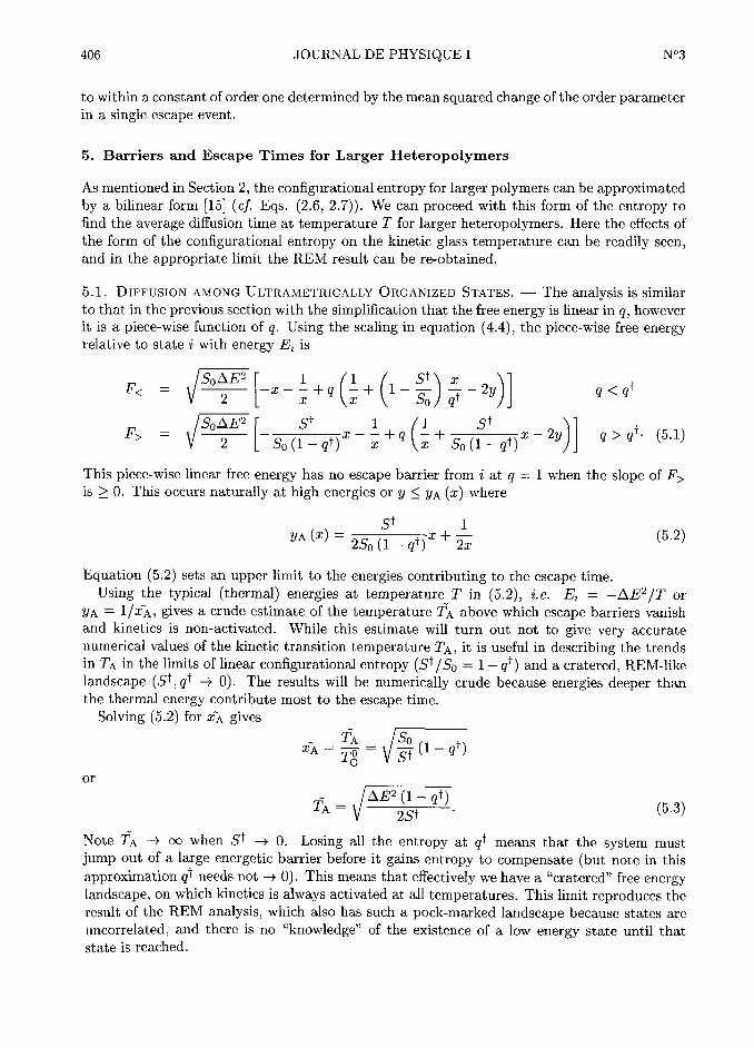
Fig. 4. The 9 possible situations of the free energies versus overlap or fraction of contacts q are
shown for the piece-wise linear approximation for the entropy.
It turns out that in these two regions the free energy may exhibit a minimum, but the onlypossible maximum will be at either qt where the low entropy formula and high entropy formula
meet or at two ends (q=
0 and q =I). A variety of cases must be analyzed since the two
minima at q[~~ and q$~~ behave differently in several different regimes. We give the detailed
discussion in Appendix D.
We can classify the form of the free energy for all possible temperatures, reference energyand overlap regimes into 9 possible situations summarized in Figure 4. Detailed results for the
various cases are shown in the Appendix D.
For the situation where the free energy in the high q regime is monotonically increasing and
the free energy in the low q regime is either monotonically increasing (situation 6), monoton-
ically decreasing (situation 5) or having a minimum (situation 4) of Appendix D, there is no
barrier to escape away from the chosen state E~. The general expressions of the parts of the
thermally averaged escape time contributed by the given ranges of energies can be written as
(assuming E(Q)=
0 and ~hE(Q)=
~hE):
~/4>,<5j,<6) =
/rap(E Tj ~o
~hE2 + TX
~~~ Vi~hET (5,14)
X is the integration limit of the energy E~, given in the Appendix D.
For the situation where free energy in the high q regime is monotonically decreasing and
free energy in the low q regime is either monotonically increasing (situation 9), monotonicallydecreasing (situation 8) or having a minimum (situation 7), there is indeed a barrier for escape.
N°3 DIFFUSION ON A CORRELATED ENERGY LANDSCAPE 411
For the situations (7) and (9) of Appendix D, the barrier is given by F(q =qt) -F(q=
I),this contribution to the escape time from the appropriate energy ranges is
r(~j~g~
=
fro exp[ ~~~"~ ]p(E, T),
~j~~ ~~, =
+ expi j~11 qtj2 ~ji qt)ierfi~E~ijjjj ~'~i isis)
where X is the integration limit for the energy E~, given in the Appendix D.
For situation (8) of Appendix D, the free energy barrier is given by F(q=
0) F(q=
I), the
escape time contribution to the given energy range is r(~j =
fro exp[ ~ ~"~ ]p(E, T).The result is:
~~~ ~~~~~~ ~°~~~~~~~~~~ ~~'~~~
where X is the integration limit for energy E~, given in the Appendix D.
For the situation where the free energy in the high q regime gives a minimum while the
free energy in the low q regime is either monotonically increasing (situation 3), monotonicallydecreasing (situation 2) or has a minimum (situation I), there is again a barrier for escapefrom the vicinity of the minimum. This gives results similar to those discussed just above.
For situation II) and (3) of the Appendix D, the free energy barrier is given byF(q
=
qt) F(q=
qmin) where qmin is the minimum of F(q) at q > qt. The escape time
contribution to the gi,>en energy range is r(~j ~~j =
fro exp[~~~"~~J~j$~~"~~'~~]p(E, T). The
result is: '
where X is the integration limit for E~, given in the Appendix D.
For situation (2), the free energy barrier is given by F(q=
0) F(q=
qmm) where qmin is
the minimum of F(q) at q > qt. The escape time contribution to the given energy range is
r(~> =fexpjf(Q=Q~J-JIQ=Qm,n)jpjE, T). The result is:
~~~ /fi(~~~~hE2) ~~~~'~ ~° ~'~~~~~~~~~~~ ~~~~~~~~~~
x exp[(~tT/(~hE~) I /T)X] (5.18)
where X is the integration limit for energy E~, given in the Appendix D.
The thermally averaged escape time from traps is contributed from the combinations of rjij,
r~2>, r~~,, T(4j, r~sj, r~sj, r~7j, rjs, and r~g, (see details give in the Appendix D).To determine the configurational diffusion coefficient, we must discuss also the integration
limits on the energy E~. There are six energy values which control whether the free energy in
region of q < qf and q > qf is monotonically increasing, decreasing or exhibits a minimum.
These six energy values are: El=
-q~~hE2 IT oT, E2=
-aT, E3=
-~hE~ IT ~tT,
E4=
-q~~hE2 IT ~tT, El#
-fiW and Eh#
fiW. The differing orders of these
energies values in different temperature ranges naturally define the integration limits for the
average escape times.
The algebraic results for escape times in the different temperature ranges are shown in
Appendix D.
412 JOURNAL DE PHYSIQUE I N°3
5.3. ILLUSTRATIVE NUMERICAL RESULTS. When we increase the size of a RHP, a bi-
linear form well approximates the configurational entropy, with parameters aand ~t
(or qf
and Stj adjusted to fit the actual entropy curve as calculated by the methods summarized
in Appendix A. To illustrate the results, the average escape time versus reduced temperature
T/TG is shown in Figure 3a for 64 mers and Figure 3b for 125 mers (in the case ofa > i and
qt < 0.5).We again see that the average escape time still does not follow the Arrhenius law. As tem-
perature is lowered, the escape time exponentially grows leading to effective kinetic trapping.The results obtained by the RSM and ultrametric models become more comparable as chain
length increases. In both cases correlation effects result in a significantly smaller escape time
than for landscapes without correlations. There exists an N dependent temperature TA (givenin the ultrametric case by Eq. (5.8)) above the thermodynamic glass transition temperature
where the dynamics becomes non-activated, and the diffusion time approaches To
6. Conclusion and Discussion
We have given adetailed analysis of the kinetics of a locally connected generalized random
energy model using the random heteropolymer as an illustration. However, the methods used
here can be readily applied to study dynamics in any rugged system, e.g. spin glasses. We can
see that the escape time for a correlated energy landscape is shorter than for an uncorrelated
surface, the search time at Tg being reduced but still exponential in the size of the system. The
distribution of escape times for an ultrametric RHP was obtained. A second temperature scale
emerges in the analyses, analogous to the temperature TA in Potts spin-glasses above which
kinetics is non-activated.
The calculation of the configurational diffusion or escape time on a non-biased correlated
energy landscape in this paper can be straightforwardly generalized to study minimally frus-
trated protein folding, where biasing towards the folded state (minimum frustration) is also
taken into account. We leave the detailed treatment of this to issue to future work.
Trap escape and unfolding are mathematically analogous, in that escaping from a largebasin or funnel on the energy landscape must involve escaping from a series of smaller basins
or funnels, as in the minimally frustrated problem. Escaping froma macro funnel requires
escape from a series of micro funnels, which requires escaping from nano funnels, etc. until the
escape time from the smallest basins or funnels reaches the fundamental microscopic time scale.
In this paper, we have renormalized all smaller basin escapes into the microscopic time scale To
A more complete treatment of diffusion on a rugged landscape would require a renormalization
group analysis for the diffusion rate in a hierarchy of funnels, which we leave to future work.
The result presented here probably overestimates the trapping escape rate while the random
energy model result clearly underestimates it. Thus for example the temperature TA, even
for 27-mers, may well exceed T(as suggested also by replica variational methods [22j. We
also point out that topological constraints in longer chains will increase the barriers over the
present illustrative results which assume no such prohibitions on kinetics.
The present methods and results, by including correlations, continue beyond the REM in
describing diffusion on a rugged landscape. The formalism can flexibly include detailed poly-meric effects only sketched here. We believe it should be a valuable next step in understandingcomplex free energy landscape models both for biopolymers and other systems.
AcknowledgTnents
We wish to thank Z. Luthey-Schulten and J. Saven for helpful discussions. Thii work is
supported in part by Grant NIH 1-R01-GM44557, and NSF grant DMR-89-20538.
N°3 DIFFUSION ON A CORRELATED ENERGY LANDSCAPE 413
Appendix A
We sketch here the calculation of the configurational entropy Sc(q), and refer the interested
reader to our earlier work [lsj.In the low overlap q limit, that is for a weakly constrained polymer, the entropy can be
decomposed into several terms:
sl"
sclfl) + ~scontact + ~smix + ~SAB' (A.i)
The first term is the entropy of all states given a specified degree of collapse. It is purely a
function of packing fraction q [19j
~Uo
~/l)
II ~~ ~~Sc in)= °g j
q°~ ~
The second term comes from the loss of entropy involved in formation of specific individual
contacts:
~hscontact=
~Nq~z [log C I + log(qz~)j (A.3)
where C=
)($)~/~, jr is the volume corresponding to the interaction range or the bond
distance between two residues, b is the persistence length of the polymer.The third term comes from the combinatorics of choosing which q, z, i N contacts overlap
with a total of z~N contacts in the collapsed state. z is the near neighbor coordination number
and N is the total number of monomers in the polymer.
~hsmix=
-Nz~ [q log q + II q) log(I q)j. (A.4)
The fourth term is associated with the fact Nz~ qNz~ contacts of the reference state must
not have been formed so that the overlap is no more than q:
~ c~
/~SAB- u
~~~dxi°~ii x~/~i IASi
The effect of confinement of the polymer chain is to change the constant in this expressionfrom C to C' where C'
=(12/7r) (jr /b~)~/~). (This term cancels to some extent the coIi1bina-
torial term.
Notice that there is a value of q less than one, qv, at which Si (qv)=
0. This value qv +~
II (z~)is rather close to where the entropy of a given contact pattern in the mean field would vanish.
It is related to the Flory [28j vulcanization value for contacts. Somewhat before this point
the polymer is overconstrained and the counting arguments used in deriving the expressionfor entropy above are invalid. For 27 mer lattices qv is close to one. But for large polymers,
qv becomes significantly less than one. The weak constraint assumption breaks down near
qv. Important configurations with q > qv must have significant clustering of the contacts or
equivalently melted out regions. The dilute contact representation is not good for such large
q, so another approximation was developed to take into account the fact that contacts must be
formed or broken simultaneously in groups. For q > qv this melting out is described by changing
the representation for low q in terms of an interacting gas of contacts to, at high q, an atomistic
description in which the reference state is one where all the contacts are formed. Here entropy
arises because contiguous parts of the frozen polymer are melted out and unconstrained. The
melted parts carry a certain entropy but there is also a combinatorial entropy associated with
the choice of the different places where a given melted piece can occur along the sequence of
the polymer. A complete form of the entropy taking into account also the end effects was thus
obtained [15j.

414 JOURNAL DE PHYSIQUE I N°3
o
~"
Q~ o
>
E; E
Fig. 5. Diagram of the GREM hierarchy used in the ultrarnetric model.
Appendix B
Consider the GREl/I hierarchy in Figure 5. Suppose we find a state with energy Ei and look
for the free energy relative to it as a function of q. We do this in order to find the escape time
from I. As in Figure 5,
E~=
fi< + fi[ and E=
fi< + fi>.
We wish to find the number of states with energy E and overlap q with state I, N (E, q, Ej).This depends on how much energy came from d<, since both E~ and E have this contribution.
For the ensemble of states with energy E~, the distribution of fi< is given by the conditional
probability distribution
p (~j~ E~)~~~ 2/~2q) ~~~ 2~)2
~ ~)
~ ~~~ ~~~~P ()~) ~ E)
~~~ 2~hE2
" ~~~ 2~~2q~~~)~
~~'~~
(Notice (B.I) has the correct limits of d (fi<) and d (fi< E~) when q ~ 0 and q ~ l respec-
tively.) Now suppose we have found a state I with E~ and a given contribution fi<. The lognumber of states having overlap q with it and energy E are
in N (E, q, E~)~
s~ (qj ~j[j (<i~iB.2j
with fi< chosen from the distribution (B.I). Using I IT=
0 In N/0E gives the free energy
F jq, 4<)"
4< TSC l~l $~~~ ~~' ~~ ~~
so that the escape time for a given realization of fi<, E~, is
T = To exp (~ ~~j ~(B.4)
where F (q*) is where the free energy has its maximum, given that it is a fluctuating quantity
since at a given q, #< fluctuates depending on which state with E~ we picked
F (q*j~ max F iqj
N°3 DIFFUSION ON A CORRELATED ENERGY LANDSCAPE 415
q* also follows a distribution for the different I having E~, which we will approximate by takingq* at its most probable value. (B.I), (B.3) and (B.4) together give the distribution for
T givenE~:
~ ~
~~ (T In + II Q*) (Ei +~)
p (~j j~ ~~~ ~~~ (~ $)~
r2~hE2q* II q*)
where r'= To exp -Sc (q*). The distribution of escape times is obtained by averaging (B.5)
over the thermal distribution of energies
E(sPT (r)
=
/dEi PT (Ei) P (rjEi) (B.6)
Eis
where E(s=
~fi@ and
j~ ~
hE~j~
~~ ~~~ " ~~~
~
2~h/
The integrand is extensive and steepest descents can be taken, with the largest contribution
to Fir) coming from
E)=
-~)~ Tln (B.7)T
(the dominant energies contributing to the escape time are always lower than the thermal
energy) and the distribution of escape times at temperature T is then given by
(T In ~) ~
~~ ~~~ "
T
~~~ 2~hE2if-
q*)~~'~~
Note that as q* ~ l, I.e. diffusion becomes a non-activated, downhill process, E) ~-~hE~ IT
arid PT IT) ~ ~ (T T0)Equations (B.I, B.3) together allow one to consider the probability distribution of the free
energy as a function of q
~ ~~~~
~~~~hE2/(1
q) ~~ ~~ ~ ~~~ ~~~ ~ ~~ ~~
~~'
~~'~~
with the mean and most probable free energy function F*(q) given by equation (2.ll).
Appendix C
The high temperature free energy (4.I) for T > v§T( is
Fm=
@(-x+ q ix 2y) +
~ (C.1)2 x
with a minimum at
q~ =12y x) (C.2)

416 JOURNAL DE PHYSIQUE I N°3
The upper bound to energies with activated barriers occurs when ql=
0 or
x
y = j
Using the thermal distribution of energies
in quation(4.2)
gives
forthe ean
cape
(T (X)) = To
which for x > v§, is of O (e~'~). So (for a large system) there are no macroscopic barriers
above v§T( (even though states with barriers exist, at these high temperatures they are not
macroscopically populated).Note that at T
=
v§T[, the mean escape time scales as a power law with system size
l~ l~~°tl1" ~°
l ~ §)~
~ l~~~~l ~~'~~
As long as the escape barrier is calculated from the melted free energy Fm in (4.I), expression(C.3) is true. This condition is that the free energy minimum is always in the melted region of
the piece-wise free energy of (4.1),or that ql (y
=Ii < qG (xi,
or x > x#=
(I + vi) /3. For
x <v§ however, expression (C.3) dictates the escape times scale exponentially with system
size IT IT))m~
O (e'~).For low temperatures such that I < x < x#, there is an energy yl (x) E(s below which the
free energy minimum is evaluated from the frozen formula Ff in (4.I). yl ix) is given by the
condition that the minima of Fm and Ff occur at the same place, I.e. q(=
q), or
~~2 ~yt (x)=
(c.5)
This value of energy splits the integral in (4.2) into two parts, thus
j~jx)j~ ~ ~ jc 61
~~
where H is the integral over higher energies x/2 < y < yl (xi, when the barrier is in the
unfrozen regime:
_~ ~~_fi
1 ~y 1 ~ 2~
~/~
~ ~~~~ ~~
~
~~~
~~~~~
X ~ ~
y=~/2
~~ ~~
Note H becomes smaller at lower temperatures, and H ~ 0 when x ~ l.
L is the contribution to the escape time from low energies yl (x) < y < I, and the barrier
must be calculated from the minimum of the frozen free energy (Ff in (4.I)), to the maximum
of the melted free energy Fm at q =0. This calculation gives
L=
~° /~~
dy exp So~9(v)
-1-y )~j
(C.8)~r ~~i x x x
2x

N°3 DIFFUSION ON A CORRELATED ENERGY LANDSCAPE 417
where
~l ~
~ ~~~
2f~ ~2
yfi)(~ + Y~ ~
~~~
+jy
(4v~ 6 ~~Y~~
For the range of temperatures I < x < x#, the largest contribution to IT (T)) in the integral is
from y =I, or the ground state energy E(s. Approximating the integral by steepest descents
gives
~ '~
2i~~~
~ ~~~~~°~ ~~~
x
~ ~ 2~ '~~~ ~~° ~~
~~'
=~xjj2~~'~~
where
g11)=
(2Vi 1) +l (2vi 1)) (1+ (2vi 1))
~~~
Gt 1.l139 9
~
~~~ /~ ~
~ ~~ ~~~ ~~
~~~ ~'~~~'
L and IT IT)) continue to increase as the temperature is lowered, until at T( (~=
l), H=
0
and
Note that the efficient in the ponent
Appendix D
For the piece-wise linear entropy function, the minimum of the free energy can be located
in different regions of q depending on the chosen Ei and temperature T. In region I, if
q[~~ < 0~ this corresponds to E~ > E2=
-To, the free energy function is monotonicallyincreasing between 0 and qt. On the other hand, if 0 < q[~~ < qt, this corresponds with
El=
-To qt~hE2 IT < Ei < -To, the free energy now has a minimum between 0 and qt.If q[~~ > l, this corresponds with Ei < El, the free energy now is monotonically decreasingbetween 0 and qt. In regime 2, if q$~~ < qt, this corresponds with E~ > E4
=-T~t
qt~hE2 IT, the free energy now monotonically increases. If qt < q$i~ < I, this correspondswith E3
=-T~t ~hE2 IT < Ei < E4, the free energy has a minimum. If q[~~ > l, this
corresponds to Ei < E3, the free energy is monotonically decreasing. So there are 3 possiblesituations for the free energy in the low q (regime I) with monotonically decreasing, minimum,
monotonically increasing behaviour and 3 possible situations for free energy at high q (regime2) with monotonically decreasing, minimum, monotonically increasing behaviour.
There are altogether 9 possible combinations of situations for the free energy as a whole in
high and low q regime. We discuss these below.
The 9 situations for the free energy are shown in Figure 4. We term them situations 11),(2), (3), (4), (5), (6), (7), (8), (9) respectively. The only differences among these 9 different
418 JOURNAL DE PHYSIQUE I N°3
F F F
, i ,
, i , ,
qo~
qo~
qo~
(i) (3) (6)
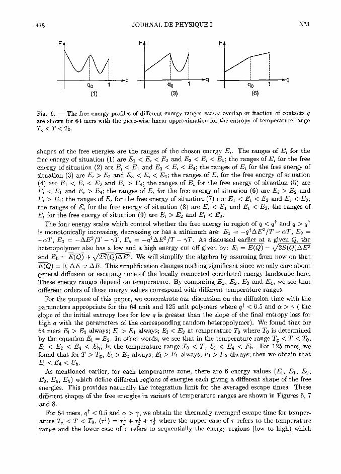
Fig. 6. The free energy profiles of different energy ranges versus overlap or fraction of contacts q
are shown for 64 mers with the piece-wise linear approximation for the entropy of temperature range
Tg < T < To.
shapes of the free energies are the ranges of the chosen energy E~. The ranges of Ei for the
free energy of situation ii are El < E~ < E2 and E3 < Ej < E4i the ranges of Ei for the free
energy of situation (2) are E~ < El and E~ < E~ < E4i the ranges of Ei for the free energy of
situation (3) are Ei > E2 and E3 < E~ < E4i the ranges of E~ for the free energy of situation
(4) are El < Ei < E2 and E~ > E4i the ranges of E~ for the free energy of situation (5) are
E~ < El and Ei > E4i the ranges of Ei for the free energy of situation (6) are Ej > E2 and
Ei > E4i the ranges of Ei for the free energy of situation (7) are El < Ei < E2 and E~ < E3i
the ranges of Ei for the free energy of situation (8) are Ei < El and Ei < E3i the ranges of
Ei for the free energy of situation (9) are Ei > E2 and Ei < E3.
The four energy scales which control whether the free energy in region of q < qt and q > qt
is monotonically increasing, decreasing or has a minimum are: El=
-Qt~hE~ IT aT, E2#
-aT, E3=
-~hE2 IT ~tT, E4=
-Qt~hE~ IT ~tT. As discussed earlier at a given Q, the
heteropolymer also has a low and a high energy cut off given by: El=
E(Q) 25(Q)~hE2
and Eh#
E(Q) + 25(Q)~hE2. We will simplify the algebra by assuming from now on that
@=
0, ~hE=
~hE. This simplification changes nothing significant since we only care about
general diffusion or escaping time of the locally connected correlated energy landscape here.
These energy ranges depend on temperature. By comparing Eli E2, E3 and E4, we see that
different orders of these energy values correspond with different temperature ranges.
For the purpose of this paper, we concentrate our discussion on the diffusion time with the
parameters appropriate for the 64 unit and 125 unit polymers where qt < 0.5 and a > ~t the
slope of the initial entropy loss for low q is greater than the slope of the final entropy loss for
high q with the parameters of the corresponding random heteropolymer). We found that for
64 mers El > E3 always; El > El always; El < E2 at temperature To where To is determined
by the equation El=
E2. In other words, we see that in the temperature range Tg < T < To,
El < E2 < E4 < Ehi in the temperature range To < T, El < E4 < Eh. For 125 mers, we
found that for T > Tg, El > E3 always; Ei > El always; El > E2 always; then weobtain that
El < E4 < Eh.
As mentioned earlier, for each temperature zone, there are 6 energy values (El, El, E2,
E3, E4, Eh) which define different regions of energies each giving a different shape of the free
energies. This provides naturally the integration limit for the averaged escape times. These
different shapes of the free energies in various of temperature ranges areshown in Figures 6, 7
and 8.
For 64 mers, qt < 0.5 and a > ~t, we obtain the thermally averaged escape time for temper-
ature Tg < T < To, (T~)=
T/ + T] + T( where the upper case ofT
refers to the temperature
range and the lower case ofT
refers to sequentially the energy regions (low to high) which
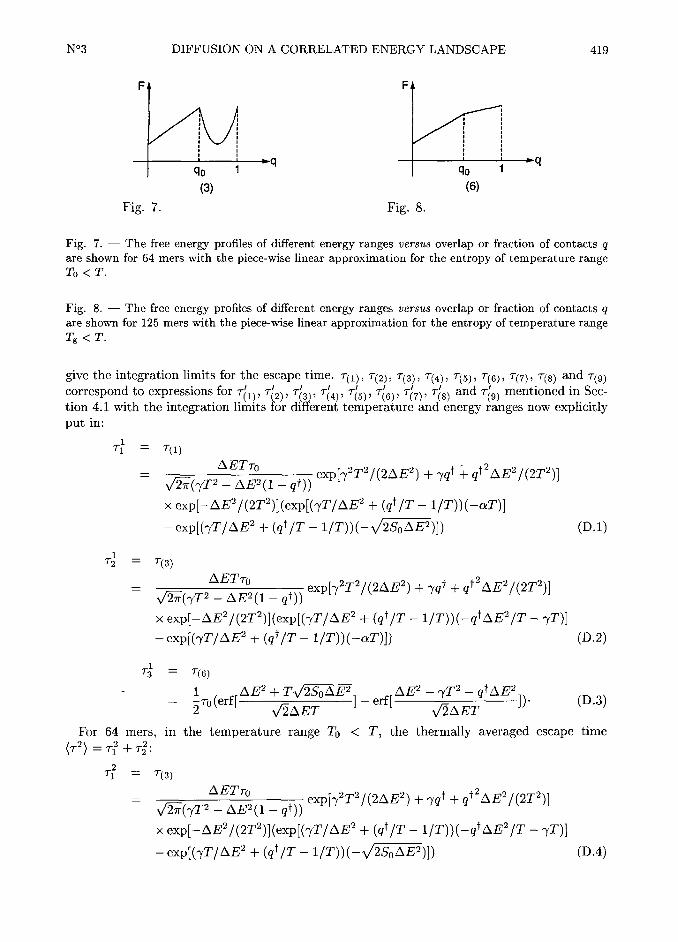
N°3 DIFFUSION ON A CORRELATED ENERGY LANDSCAPE 419
' ,
qo I qo
(3) (6)
Fig. 7. Fig. 8.
Fig. 7. The free energy profiles of different energy ranges versus overlap or fraction of contacts q
are shown for 64 mers with the piece-wise linear approximation for the entropy of temperature rangeTo < T.
Fig. 8. The free energy profiles of different energy ranges versus overlap or fraction of contacts q
are shown for 125 mers with the piece-wise linear approximation for the entropy of temperature range
Tg < T.
give the integration limits for the escape time. T~i), T~2j, Tj~,, T~4,, T~s,, T~5), T~7>, T~s) andT~gj
correspond to expressions for T(~j, T'~j, T(~ , T(~~, T(~~, T(~j, T(~~, T(j andT(g~
mentioned in Sec-
tion 4.I with the integration limits )or different temperature and energy ranges now explicitly
put in:
T/# Tjl)
~~~~~)j expjrf~T~ /j2~E~j + ~fqt I qt~~E~ /(2T~jj
xe)j)-~E~
j2~~jjje~~jj~fT/~E~+ jqt IT I /Tjjj-aTjj
expjj~fT/~E~ + (qt IT I /Tjjj- @wjjj jD,lj
T(# T~3)
~~~~@)j
~~ ~~~
exPi'i~T~/(2~E~) +'iq~ + q~~~E~/(2T~)1
xexp)-~E2
j2T2)j(e~pjjr~T/~E2+ iqt IT i /T)) (-qt~E2 IT r~T)j
exPil'iT/~E~ + (q~/T I/T))(-°T)i) iD.2)
T(# T~6)
1 ~hE2 + TfiW ~hE2 ~tT2 qt~hE~2~~~~~~ v§~hET ~~~~ v§~hET ~~
~~'~~
For 64 mers, in the temperature range To < T, the thermally averaged escape time
(T~)#
T/ + Tjl
T/# T~3)
/fi(~tT2~~~~2 ii qt)j~~~~'~~~~~~~~~~~ ~'~~~ ~ ~~~~~~~~~~~~~
xexp[-~IE~ /(2T~)j (exp[(~tT/~hE~ + (qt IT 1IT) )(-qt~lE~ IT ~tT)]
expii~tT/~hE~ + iqt IT i/Tii i-@Wii) iD.4)

420 JOURNAL DE PHYSIQUE I N°3
Tj" T<6j
~°~~~~~~~~ ~j~h~~~~~~~~~~~~ ~~E/~~~~
~~~~'~~
For 125 mers, in the temperature range T > Tg, the thermally averaged escape time
(T)# Tl +T2~
Ti = T13j
/fi(~tT2~~~~ (1 qt))~~~~'~~~~~~~~~~~ ~'~~~ ~ ~~~~~~~~~~~~~
xexp[-~hE~ /(2T~)j(exp[(~tT/~hE~ + (qt IT I IT)) (-qt~hE~ IT ~tT)j
expii~tT/~E~ + iqt/T i/T))i-@W)i) IDfi)
~2 " ~<6j
~~~~~~~~~ ~j~h~~~~~~~~~~~~ j~~E/~~~~~~ ~~ ~~
References
[Ii Frauenfelder H., Sligar S. and Wolynes P.G., Science 254 (1991) 1598 and references
therein; Frauenfelder H., Wolynes P-G-, Phys. Today 47 (1994) 58; Wolynes P.G., in
"Spin Glass and Biology", Stein, Ed., (World Sci entific Pub., 1992) pp. 225-259.
[2j MAzard M., Parisi G., Virasoro M.A., Spin Glass Theory and Beyond (World Scientific
Pub., 1987).
[3] Bryngelson J-D- and Wolynes P.G., Proc. Nat(. Acad. Sci USA 84 (1987) 7524; J. Phys.Chem. 93 (1989) 6902.
[4] Onuchic J.N., Wolynes P-G-, Luthey-Schulten Z.A. and Socci N-D-, Proc. Nat(. Acad. Sci.
92 (1995) 3626.
[5j Socci N-D-, Onuchic J-N- and Wolynes P.G., J. Chem. Phys. 104 (1996) 5860-5868.
[6j Goldstein R-A-, Luthey-Schulten Z-A- and Wolynes P-G-, Proc. Nat(. Acad. Sci. USA 89
(1992) 9029.
[7] Bouchaud J-P. and Dean D-S-, J. Phys. I France 5 (1995) 265-286.
[8j DeDominicis C., Orland H., LainAe F., J. Phys. Lett. Ikance 46 (1985) L463; KoperG-J-M-, Hilhorst H-J-, Europhys. Lett. 3 (1987) 1213.
[9j Bryngelson J-D-, Onuchic J-N-, Socci N-D-, Wolynes P-G-, Proteins Struct. Funct. Genet.
21 (1995) 167 and references therein.
[10] Wolynes P-G-, Onuchic J.N., D. Thirumalai D., Science 267 (1995) 1619; Chan H.S., Dill
K.A., J. Chem. Phys. loo (1994) 9238; Abkevich V.I., Gutin A.M., Shakhnovich E.I., J.
Chem. Phys. 101 (1994) 6052.
[iii Derrida B., Phys. Rev. B 24 (1981) 2613.
[12] Gross D-J-, Kanter I. and Sompolinsky H., Phys. Rev. Lett. 55 (1985) 304.
[13] Shakhnovich E.I. and Gutin A-M-, Europhys. Lett. 8 (1989) pp. 327-332.
[14] Sasai M. and Wolynes P.G., Phys. Rev. Lett. 65 (1990) 2740; Shakhnovich E-I- and Gutin
A.M., Biophys. Chem. 34 (1989) 187; Garel T. and Orland H., Europhys. Lett. 6 (1988)307.
N°3 DIFFUSION ON A CORRELATED ENERGY LANDSCAPE 421
[15] Plotkin S., Wang J., Wolynes P-G-, Phys. Rev. E 53 (1996) 6271.
[16] Plotkin S., Wang J., Wolynes P-G-, J. Chem. Physlo6 (1997) 2932-2948.
[17j Levinthal C., Proceedings of Meeting at Allerton House, P. DeBrunner, J. Tsibris and
E. Munck, Eds. (Univ. of Illinois Press, 1969) p. 22.
[18j Derrida B., J. Phys. Lett. 46 (1985) L401; Derrida B. and Gardner E., J. Phys. C19
(1986) 2253.
[19j Bryngelson J.D. and Wolynes P.G., Biopoiymers 30 (1990) 177.
[20j Kirkpatrick T.R. and Wolynes P.G. Phys. Rev. B 36 8552(1987) 8552; Kirkpatrick T.R.,Thirumalai D. and Wolynes P-G-, Phys. Rev. A 40 (1989) 1045.
[21j Kirkpatrick T-R- and Wolynes P.G., Phys. Rev. A 35 (1987) 3072.
[22j Takada S. and Wolynes P.G., Phys. Rev. E (to appear).
[23j Saven J.G., Wang J. and Wolynes P.G., J. Chem Phys 101 (1994) 11037-11043; Wang J.,Saven J.G. and Wolynes P-G-, J. Chem. Phys. 105 (1996)11276-11284.
[24j Hagen S.J., Hofrichter J., Szabo A. and Eaton W.A., Proc Nat(. Acad. Sci. 93 (1996)l1615-l1617.
[25j Unless otherwise indicated, all entropies have dimensions of Boltzmann's constant kB.
[26j Unless otherwise indicated, all temperatures have units of energy, with Boltzmann's con-
stant kB included in the definition of T.
[27j Koretke K-K-, Luthey-Schulten Z. and Wolynes P-G-, Protein Sci. 5 (1996) 1043-1059.
[28j Flory P-J, Chem. Rev. 35 (1944) 51; J. Chem. Phys. 18 (1950) 108.