Consumable Double-Electrode GMAW Part II: …ymzhang/Papers/2007 Welding Journal...1 Consumable Double-Electrode GMAW Part II: Monitoring, Modeling, and Control by Kehai Li and Y.M

1

Consumable Double-Electrode GMAW

Part II: Monitoring, Modeling, and Control

by

Kehai Li and Y.M Zhang

Kehai Li ([email protected], PhD student,) and Y. M. Zhang ([email protected],

Professor of Electrical Engineering and Corresponding Author) are with Center for

Manufacturing and Department of Electrical and Computer Engineering, University of

Kentucky, Lexington, KY 40506.

Abstract

Consumable DE-GMAW is an innovative welding process, which can significantly

increase the deposition rate without raising the base metal heat input to an undesired level.

To be qualified as a practical manufacturing process, feedback control is required to

assure the presence and stability of the bypass arc. To this end, the bypass arc voltage

was selected to monitor the state of the bypass arc. Further, the authors proposed an

interval control algorithm for models whose parameters are bounded by given intervals.

This algorithm does not require the specific values for parameters, but only their intervals,

which can be identified through a selected set of experiments. By conducting step

responses under different conditions, a few models were obtained and the parameter

intervals were determined and enlarged to increase the stability margin. Using the

obtained parameter intervals in the interval control algorithm, closed-loop control

2

experiments have been conducted to verify the effectiveness of the proposed control

system for the consumable DE-GMAW process.

Keywords: Double-Electrode, Arc Welding, Melting Rate, Interval Model, Welding

Controls, Heat Input

1. Introduction

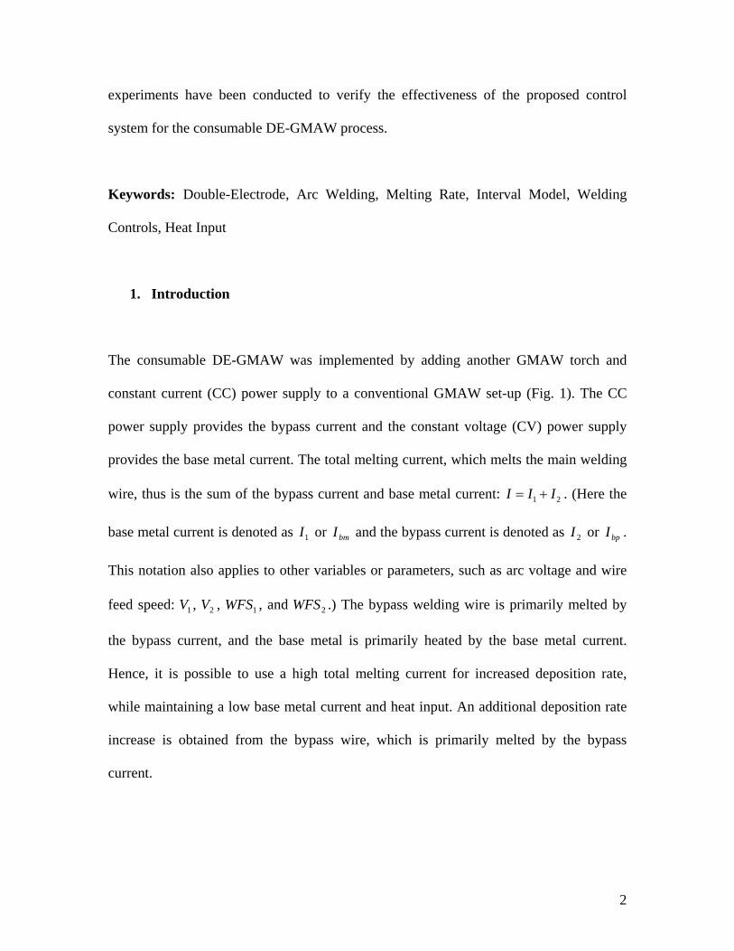
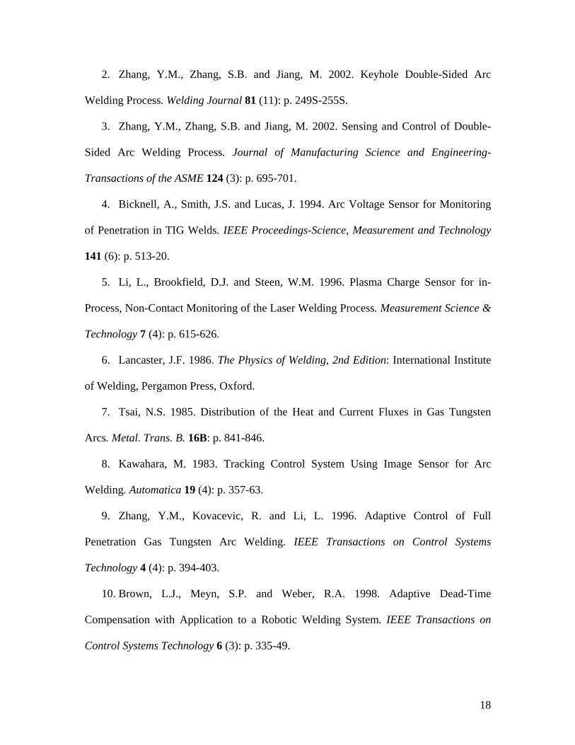
The consumable DE-GMAW was implemented by adding another GMAW torch and

constant current (CC) power supply to a conventional GMAW set-up (Fig. 1). The CC

power supply provides the bypass current and the constant voltage (CV) power supply

provides the base metal current. The total melting current, which melts the main welding

wire, thus is the sum of the bypass current and base metal current: 1 2I I I= + . (Here the

base metal current is denoted as 1I or bmI and the bypass current is denoted as 2I or bpI .

This notation also applies to other variables or parameters, such as arc voltage and wire

feed speed: 1V , 2V , 1WFS , and 2WFS .) The bypass welding wire is primarily melted by

the bypass current, and the base metal is primarily heated by the base metal current.

Hence, it is possible to use a high total melting current for increased deposition rate,

while maintaining a low base metal current and heat input. An additional deposition rate

increase is obtained from the bypass wire, which is primarily melted by the bypass

current.

3

However, as discussed in Part I, without proper control the process can only remain

stable when the welding parameters are carefully selected and do not vary in large ranges.

If the process becomes unstable and the bypass arc extinguishes periodically, the bypass

loop would break and all the melting current would be imposed onto the base metal. Such

a large base metal current can burn-through and damage the workpiece. Thus to assure

the consumable DE-GMAW process functions properly, its stability must be controlled

and guaranteed. To this end, an appropriate signal must be found to characterize the

process stability. This signal must accurately reflect the process stability and be

monitored conveniently in a manufacturing environment. Then a process model can be

obtained to design a suitable control algorithm. Hence, this paper (Part II) devotes to the

monitoring, modeling, and control of the consumable DE-GMAW process.

2. Stability Monitoring

2.1 Vision Signal

The most direct indication of stability is obtained by monitoring the bypass arc,

especially the location of the tip of the bypass welding wire in relation to the main arc.

Experiments show that when the bypass arc is stable, the tip of the bypass welding wire

must be close enough to the main arc. However, machine vision (Ref.1) requires an

imaging system, which should be installed to and move with the welding torch. This

makes the welding system complicated. Machine vision may not be the most preferable

method for welding processes.

4

2.2 Sound Signal

Usually there is a characteristic sound in welding associated with each particular

operating mode. For example, in plasma arc welding there is a characteristic sound when

the keyhole is established. In GMAW, the sound can vary quite drastically and is

dependent on the mode of metal transfer. A similar phenomenon was observed in the

consumable DE-GMAW. For instance, when the bypass arc was unstable, the sound was

hard and accompanied by spatters. But once the bypass arc became stable, the metal

transfer became into spray transfer mode because of the high melting current, thus there

was no spatters and sharp sound.

2.3 Thermal Signal

Thermal signal reflects the temperature field, which heavily depends on the distance for a

specific thermal point. Take the consumable DE-GMAW process as an example, the

bypass arc can be seen as a thermal point. In the axis direction of the bypass welding wire,

different positions will have different temperatures depending on their distances from the

welding arc. Thus, a fixed position thermal coupler theoretically can be used to monitor

the relative movement of the tip of the bypass welding wire.

5

2.4 Current Signal

Current signal is often used in welding processes. It has been successfully used in double-

sided arc welding (DSAW) to detect the establishment of the keyhole (Ref.2, 3). In the

DE-GMAW the bypass current can tell the existence of the bypass arc. However, because

the bypass power supply is a CC welding machine, the bypass current does not change

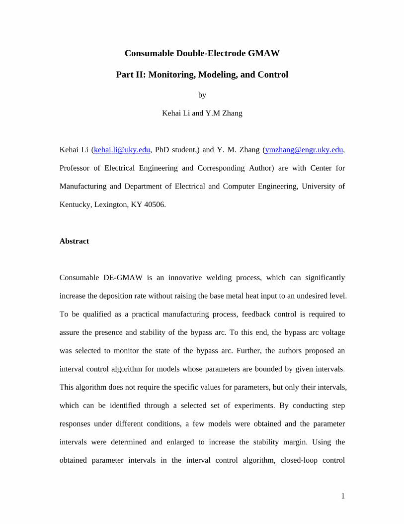
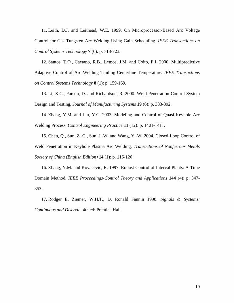
with the arc length. Fig. 2 illustrates an experiment with the following parameters: 1WFS

= 14m/min (550IPM), 1V = 36volts, 2WFS = 5.1m/min (200IPM), and 2I = 150amps.

The bypass current was set to a high value to make the bypass arc unstable. It can be seen

that the bypass current was present once the bypass arc was ignited. When the bypass arc

became longer and longer, the bypass current did not change. Once the bypass arc

extinguished, the bypass current dropped to zero abruptly. Thus, the bypass current can

only indicate two discrete states: bypass arc on or bypass arc off, but not the trend to

become unstable.

2.5 Voltage Signal

Arc voltage signals, arc length (Ref.4, 5) for example, are often used to monitor welding

processes. Normally, the arc voltage is proportional to the arc length. The following can

be observed during DE-GMAW experiments. (1) The bypass arc voltage is equal to the

main arc voltage when the bypass welding wire touches the workpiece. This happens

when the bypass wire feed speed is too fast; (2) When the length of the bypass arc

6

increases, 2V increases as illustrated in Fig. 2; (3) There is an optimal 2V which appears

to establish an optimal operating point to stabilize the process; (4) When the bypass arc

tends to extinguish, 2V tends to increase to a high level. The arc voltage can thus reflect

the state of the bypass arc. The state of the bypass arc can be predicted from the bypass

arc voltage. Hence, the bypass arc voltage may be used to characterize the stability of the

consumable DE-GMAW process.

3. Process Analysis

As discussed earlier, the consumable DE-GMAW process has two parallel arcs: the main

arc established between the main welding wire and the workpiece, and the bypass arc

established between the main welding wire and the bypass welding wire. The main

welding wire is the common anode of the two arcs, and its melting is determined by the

sum of the two currents or the total current.

When the main wire feed speed ( 1WFS ) and arc voltage ( 1V ) are given, the total current

is approximately fixed. The use of the CV power supply assures a constant distance from

the tip of the main welding wire to the workpiece (between them 1V is measured). This

distance is not affected by variations in the bypass arc length.

The bypass welding wire is primarily melted by the cathode heat of the bypass arc. The

bypass current ( 2I ) needed for a given bypass wire feed speed is approximately fixed,

even though a perturbation is introduced for 2WFS . In fact, if 2WFS is increased, the

7

cathode heat would become insufficient to melt the bypass welding wire. As a result, the

distance from the contact tube to the tip of the bypass welding wire will increase, and the

extension of the bypass welding wire increases. In the meantime, the resistive heat

(proportional to 22I and the stickout length (Ref.6, 7)) also increases. If 2WFS is

decreased, the cathode heat will tend to melt the bypass welding wire faster, but a

reduced extension will reduce the resistive heat. In both cases, new equilibriums will be

re-established at different locations, but the measured 2V will be changed. The process

shifts from the optimal condition. To maintain the stability, the authors proposed to adjust

the cathode heat to maintain the bypass welding wire at its optimal location in relation to

the main welding wire.

The above discussion and analysis suggest that the process to be controlled for the bypass

arc stability can be defined as a dynamic system with 2V as the output and 2I as the input.

It appears that the dynamic model, which correlates the input and output, may be affected

by the bypass wire feed speed, but possible effects from 1WFS and 1V setting should not

be significant. This implies that the dynamic model established using a particular 2WFS

may be just a local model. When a different 2WFS is used, the process dynamics may

subject to change.

As can be seen, the control of the bypass arc stability requires the bypass current be

adjusted in real-time. Although the base metal current will change with the bypass current,

the stability of the main arc will be maintained by the CV power supply. When 2WFS

8

and the desired 2V setting are given, the required 2I is approximately fixed and the real-

time adjustment of 2I will be made in a relatively small range. Then the base metal

current does not change significantly. For most applications, no further control is needed

for the base metal current because small variations should be tolerated. If the base metal

current needs to be controlled strictly, 2WFS can be adjusted together with 2I and will

not be discussed here. This study focuses on the most fundamental issue: the control of

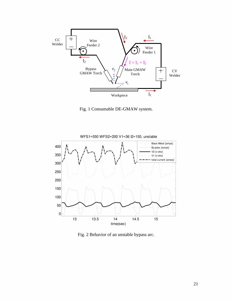
the bypass arc stability. To this end, a control algorithm needs to be designed to adjust the

bypass current to maintain the bypass arc voltage 2V at a desired optimal value while

1WFS , 2WFS , and 1V are constants. Fig. 3 shows the closed-loop control system to be

developed. The solid arrow associated with 2WFS implies that 2WFS may possibly

affect the dynamics of the process, and the dashed arrows associated with 1WFS and 1V

indicate that the possible effects of 1WFS and 1V on the dynamics are insufficient and

negligible.

4. Control Algorithm

For manufacturing systems, their models are typically affected by the manufacturing

conditions. Experiments can be conducted to identify different models with different sets

of manufacturing conditions. These models represent the process dynamics in those

manufacturing conditions. If all models have the same structure but different values of

parameters, an interval (a minimal value and a maximal value) can be found for each

parameter in the model structure. The model can be described using the bounded known

intervals for the given ranges of manufacturing conditions. This type of model is referred

9

to as an interval model. The interval model control algorithm is a standard program and

does not require any design work. Hence, unlike other techniques such as adaptive

control, neural network, and predictive control.(Ref.8-15), the interval model based

modeling and control is suitable for welding engineers without systematical training in

control. It can be used even if the intervals are relatively small. In particular, the intervals

can be artificially enlarged to increase the stability margin of the closed-loop system.

The original interval model control algorithm (Ref.16) is based on linear systems

described using an impulse response model:

∑=

−=N

jjkk ujhy

1)( (1)

where k is the current instant, ky is the output at time k , k ju − is the input at

)( jk − )0( >j , while N is the system order and sjh ' )( are the real parameters of the

impulse response function. ( ) ' (1 )h j s j N≤ ≤ are unknown but bounded by the intervals:

) ..., ,1( )()()( maxmin Njjhjhjh =≤≤ (2)

Where )()( maxmin jhjh ≤ are the minimum and maximum value of ( ) ' (1 )h j s j N≤ ≤

and known. That is, if the parameters of the actual model are bounded by the (nominal)

intervals, it is guaranteed *lim yykk=

+∞→, where *y is the set-point of the output. The

objective of the control algorithm is to determine the feedback control action ku such that

the closed-loop system achieves the given set-point.

10

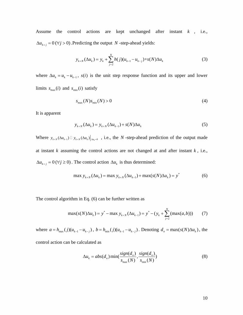
Assume the control actions are kept unchanged after instant k , i.e.,

)0( 0 >∀=∆ + ju jk .Predicting the output N -step-ahead yields:

12

( ) ( )( )+ ( ) N

k N k k k k j kj

y u y h j u u s N u+ − −=

∆ = + − ∆∑ (3)

where 1k k ku u u −∆ = − , )(is is the unit step response function and its upper and lower

limits )(max is and )(min is satisfy

max min( ) ( ) 0s N s N > (4)

It is apparent

kkNkkNk uNsuyuy ∆+∆=∆ −++ )()()( 1 (5)

Where 1 0( ) ( ) kk N k k N k uy u y u+ − + ∆ =∆ ∆ , i.e., the N -step-ahead prediction of the output made

at instant k assuming the control actions are not changed at and after instant k , i.e.,

)0( 0 ≥∀=∆ + ju jk . The control action ku∆ is thus determined:

*1 ))(max()(max)(max yuNsuyuy kkNkkNk =∆+∆=∆ −++ (6)

The control algorithm in Eq. (6) can be further written as

* *1

2

max( ( ) ) max ( ) ( (max( , )))N

k k N k kj

s N u y y u y y a b+ −=

∆ = − ∆ = − +∑ (7)

where max 1( )( )k k ja h j u u− −= − , min 1( )( )k k jb h j u u− −= − . Denoting max( ( ) )n kd s N u= ∆ , the

control action can be calculated as

max min

( ) ( )( ) min( , )( ) ( )

n nk n

sign d sign du abs ds N s N

∆ = (8)

11

where ( )sign is a function to return the sign of its parameter. Then, the output of the

control algorithm can be calculated as 1k k ku u u−= + ∆ .

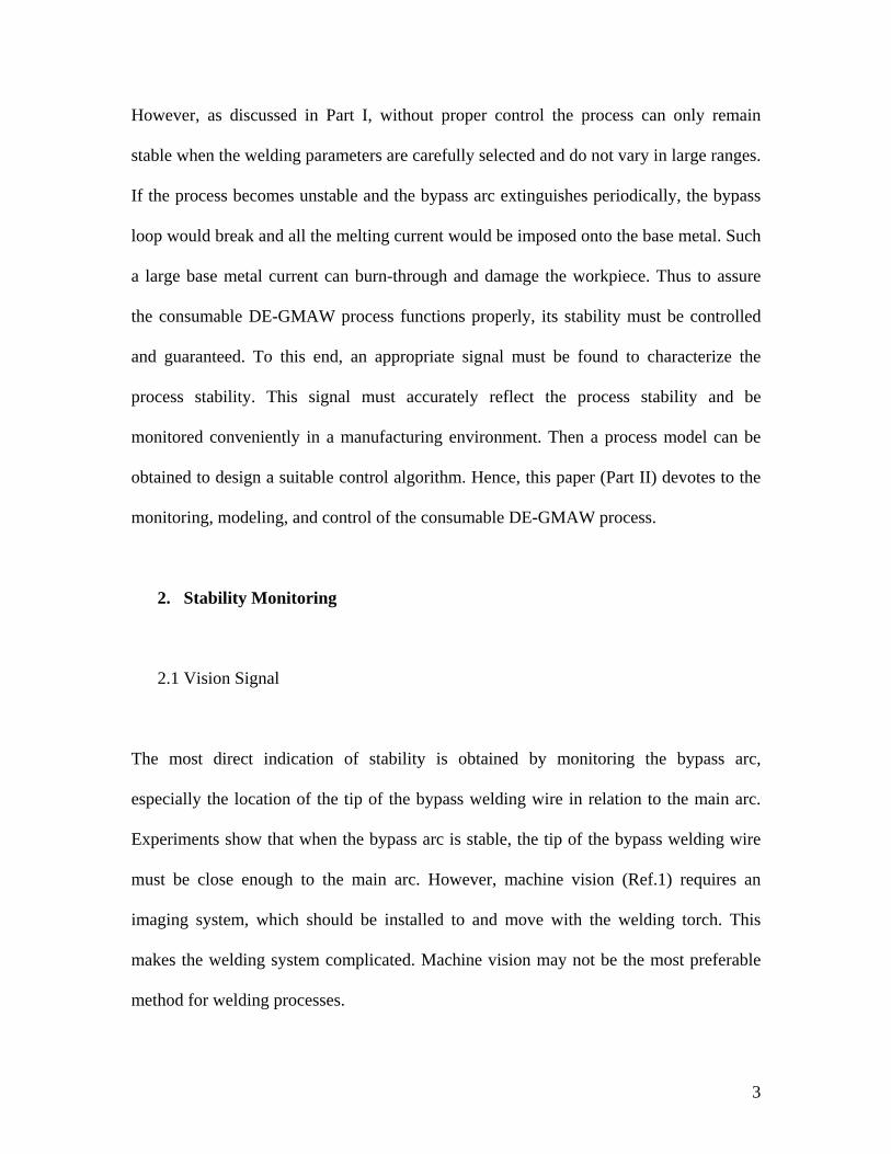
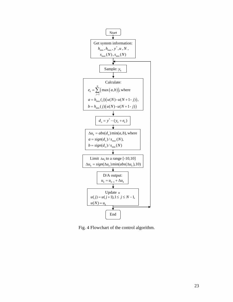
Fig. 4 illustrates the control algorithm described above. In the control system, ku∆ was

limited to [-10amps 10amps] in each step to avoid an abrupt change in the bypass current.

Obviously, an abrupt change in welding current will burn the contact tip. Once the new

output ku is calculated, the input history u must be updated.

5. Process Modeling

To model the consumable DE-GMAW process, step response experiments have been

conducted with 1WFS equal to 14.0m/min (550IPM) and 1V equal to 36volts. Because the

bypass wire feed speed may affect the process dynamics, experiments were conducted in

major ranges of the bypass wire feed speed: 16.5m/min (650IPM) at the high range,

10.2m/min (400IPM) in the moderate range, and 5.1m/min (200IPM) in the low range.

The main welding wire as well as the bypass welding wire was 1.2mm (0.045in.)

diameter low carbon steel (ER70s-6). Shielding gases (pure argon) was provided through

the main torch at a flow of 18.9 liter/min (40 CFH).

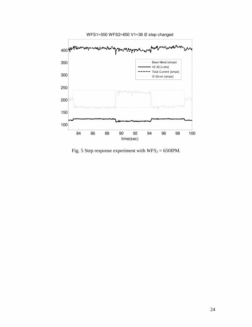
Fig. 5 illustrates an experiment in the high range of the bypass wire feed speed (650IPM).

It can be seen that step changes in the bypass current resulted in immediate changes in the

base metal current as well in the bypass arc voltage. However, the total melting current

did not change with the bypass current.

12

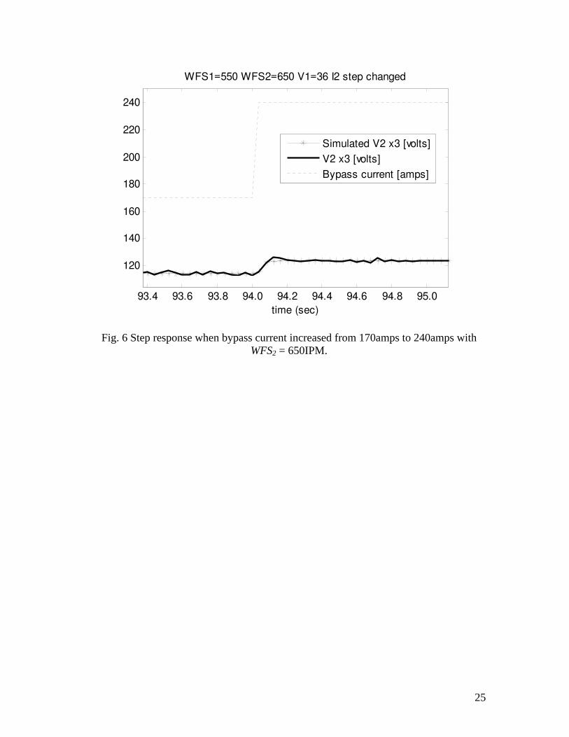
Fig. 6 shows the step response when the bypass current increased from 170amps to

240amps. A careful examination indicates (1) the process can be approximated by a first

order system; (2) the bypass voltage 2V increased 3.11volts; (The signal 2V was

multiplied by a factor 3 such that it can be plotted together with other signals.) (3) the

time constant is 0.0228second. Hence, the resultant model can be expressed as a transfer

function ( ) 0.0444 (0.0228 1)H s s= + , with a static gain equal to 0.0444 V/A. Comparing

the simulated 2V plot to the actual 2V plot in Fig. 6 suggests that the first order system

has accurately modeled the process.

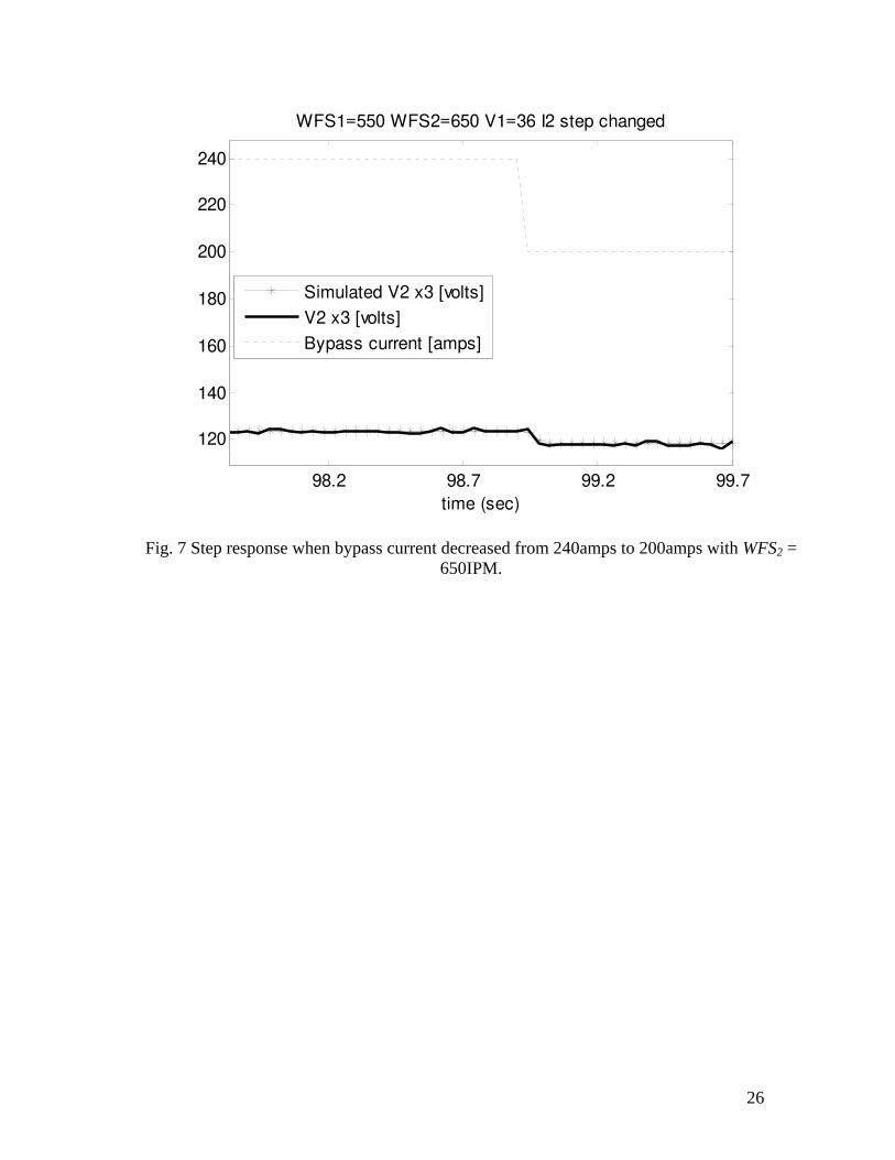
In another segment of Fig. 6, the bypass current was decreased from 240amps to

170amps. This step response can be modeled as another first order system

( ) 0.0431 (0.0295 1)H s s= + , and comparing the simulated 2V plot to the actual 2V plot

in Fig. 7 suggests that the first order system has accurately modeled the process.

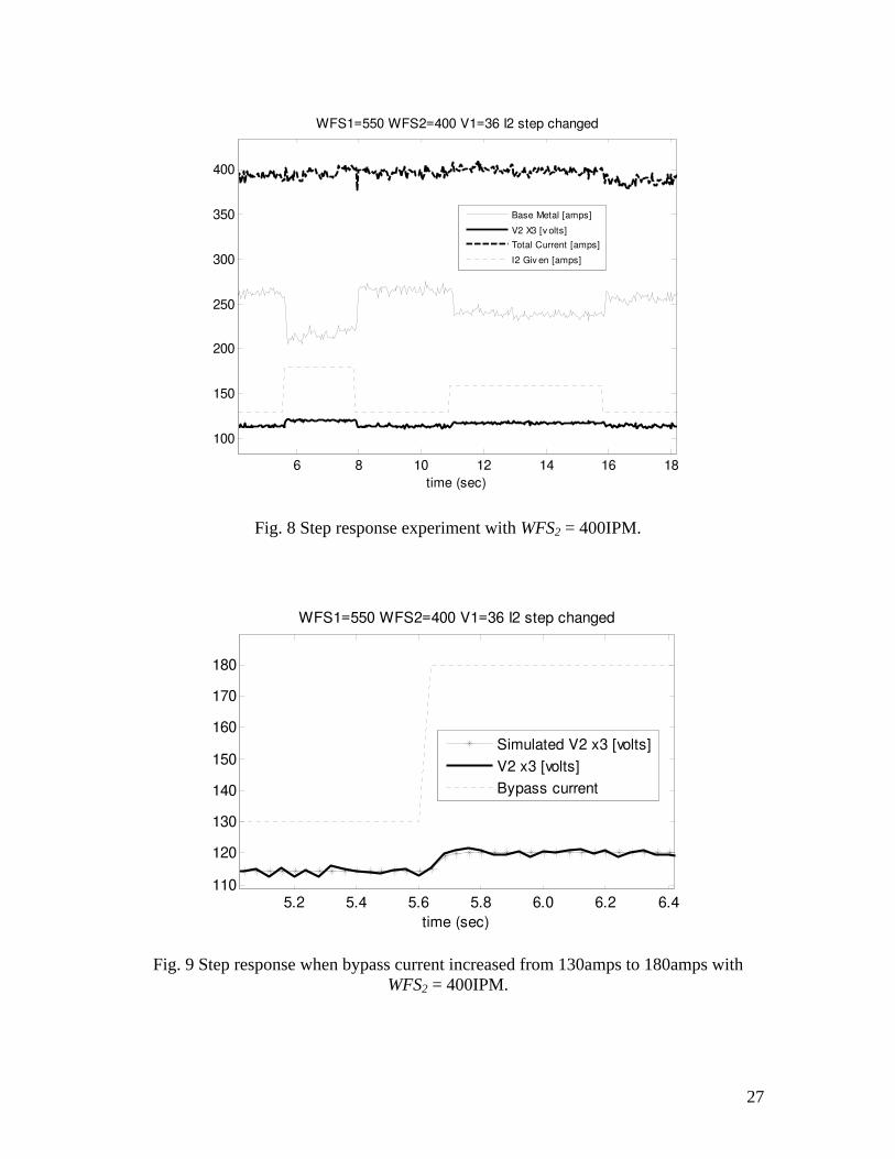
Fig. 8 shows an experiment in the moderate range of the bypass wire feed speed. It can be

seen the total current was maintained around 395amps even though the bypass current

changed. Also, the base metal current changed with the bypass current.

Fig. 9 gives the segment when the bypass current increased from 130amps to 180amps. It

can be seen that the system can be modeled as ( ) 0.0395 (0.0228 1)H s s= + for the

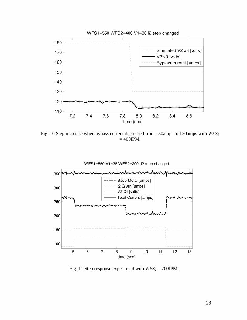
moderate bypass wire feed speed. In the segment shown in Fig. 10, the bypass current

13

decreased from 180amps to 130amps. Obviously, the system is still a first order system

with a transfer function ( ) 0.04 (0.0258 1)H s s= + .

Another step response experiment in Fig. 11 was performed with a bypass wire feed

speed equal to 5.1m/min (200IPM). In this experiment, the main wire feed speed was still

14m/min (550IPM) and the main arc voltage was 36volts. (The voltages in Fig. 11 - 13

were multiplied with a factor 4.) It can be seen the total current was not changed when

the bypass current changed. However, the bypass voltage did change with the bypass

current (at a constant bypass wire feed speed).

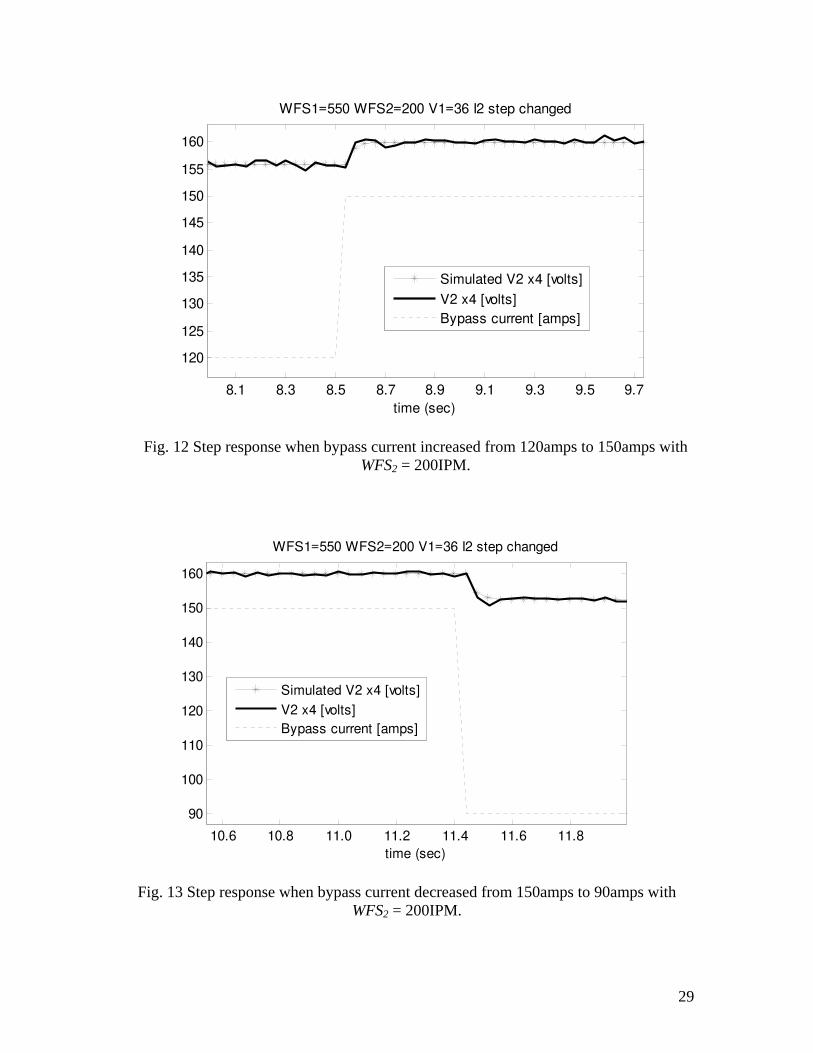
In Fig. 12, the bypass current increased from 120amps to 150amp. The system can be

modeled as ( ) 0.0449 (0.0270 1)H s s= + . A step response simulation was done and

compared to the experimental data as illustrated in Fig. 13. Similarly, when the bypass

current decreased from 150amps to 90amps, the system can be modeled as

( ) 0.0414 (0.0277 1)H s s= + . The good agreement between the simulated 2V plot and the

actual 2V plot in Fig. 12 and 13 verifies that the first order system has accurately

modeled the process.

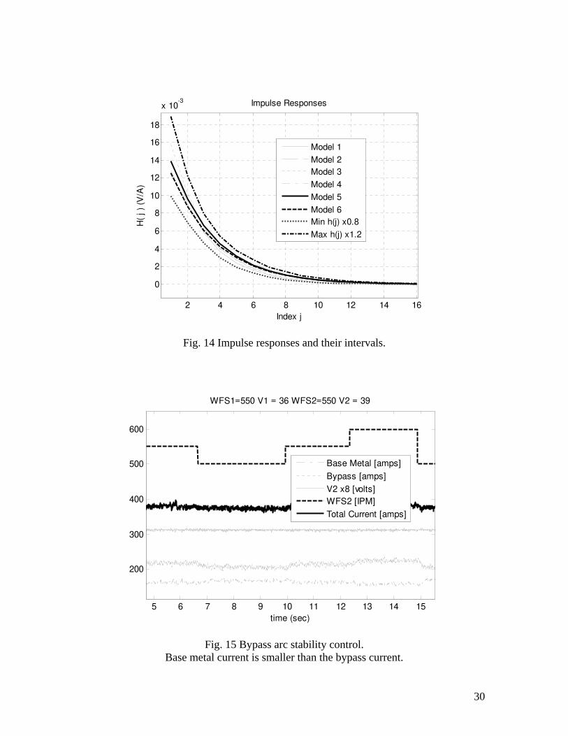
The six transfer functions can be easily converted to impulse responses ( ) 'h j s by taking

the inverse Laplace transform (Ref.17). These impulse responses are required by the

interval model control algorithm and shown in Fig. 14 with a sample period of T=0.01

second. The minimum and maximum of ( ) 'h j s were found and formed two curves

jjh ~)(min and jjh ~)(max . The two curves can be used to give the intervals for the

14

impulse responses. To improve the stability margin critical applications, the intervals can

be artificially enlarged from [ )(min jh )(max jh ] to [0.8* )(min jh 1.2* )(max jh ]. With the

enlarged intervals, the truncation of the impulse responses would cause no effect on the

stability of the closed-loop system. Using these intervals, the control algorithm described

in Eq. (6) and Fig. 4 can be used to calculate the manipulator 2I based on the feedback of

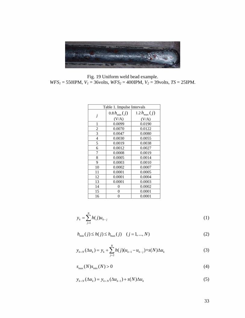
2V . In addition, the intervals in Table 1 were obtained with a bypass wire feed speed

from 5.1m/min (200IPM) to 16.5m/min (650IPM). The closed-loop system using these

intervals would work when the bypass current varies in a large range.

6. Control Experiments

6.1 Experimental setup

The consumable DE-GMAW set-up illustrated in Fig. 1 has been implemented at the

University of Kentucky by adding a second GMAW torch and CC power supply to a

standard GMAW system. A current sensor was used to feedback the base metal current to

the control system. A voltage sensor was utilized to feedback the bypass arc voltage. A

second current sensor was used to monitor the bypass current, while an additional voltage

sensor was connected to monitor the main arc voltage. The control signals passed D/A

boards and isolation boards before they acted on the power supplies. An Olympus high-

speed camera equipped with a narrow-banded light filter (central wavelength: 940nm,

band width: 20nm) was used to record the arc behavior and metal transfer. During

experiments, the torches moved together from right to left at a travel speed (TS) of

15

0.64m/min (25IPM). The workpiece was low-carbon steel with a thickness of on 0.5 inch

(12.7mm). Pure argon was used as shielding gases only through the main GMAW torch.

6.2 Interval Model Control Experiments

Experiments have been performed to verify the proposed control system for the bypass

arc stability. The main wire feed speed was set to 14.0m/min (550IPM), but the bypass

wire feed speed was changed during experiments. The expected output for the bypass

voltage was 39volts while the main arc voltage was 36volts.

In Fig. 15, the bypass wire feed speed was fluctuated around 14m/min (550IPM). It can

be seen that the bypass voltage was controlled around 39volts even though the bypass

wire feed speed changed. An increase in the bypass wire feed speed resulted in an

increase in the bypass current due to the closed-loop control. As a result, the feeding-

melting balance can be maintained, and a stable bypass arc was obtained. As expected,

the total current maintained constant and smooth because of the corresponding change in

the base metal current.

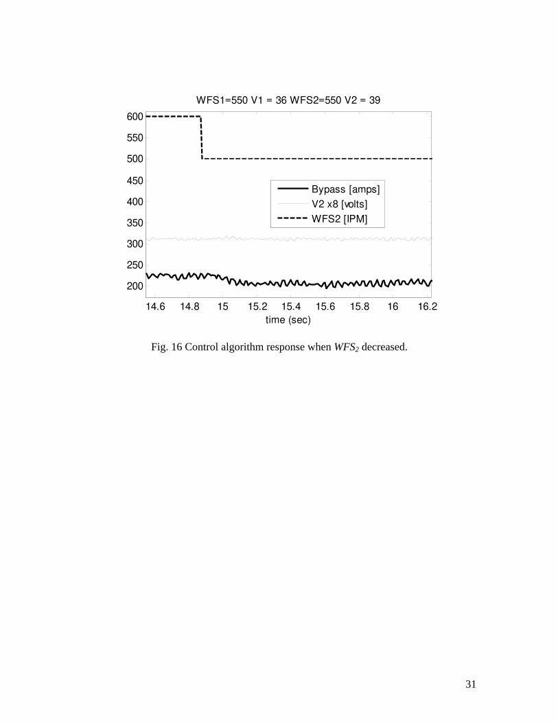
A segment of Fig. 15 was zoomed in to show the response characteristics of the control

algorithm. It can be seen that when the bypass wire feed speed decreased from 15.2m/min

(600 IPM) to 12.7m/min (500IPM), the bypass arc voltage was controlled without any

obvious change. This verified the appropriate and rapid adjustment in the bypass current

from the control algorithm.

16

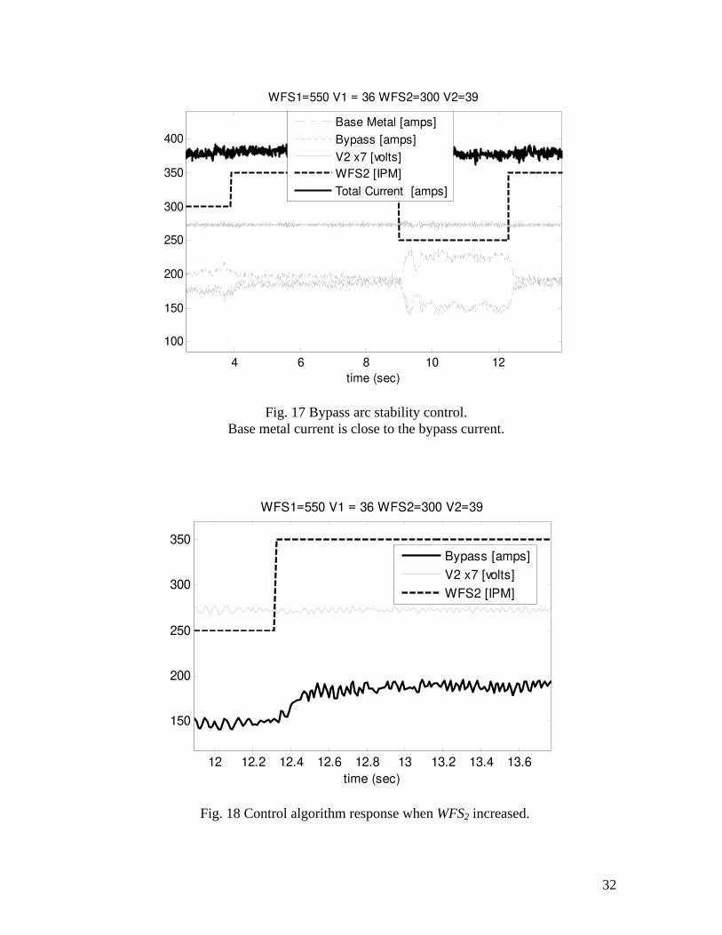
A similar experiment was done by decreasing the bypass wire feed speed to a lower level

around 7.6m/min (300IPM). The experimental results are plotted in Fig. 17. It can be

seen that the bypass arc voltage can be controlled at the desired voltage (39volts).

Furthermore, the changes in the bypass wire feed speed did not affect the total melting

current or the bypass voltage.

When the bypass wire feed speed increased abruptly from 6.4m/min (250IPM) to

8.9m/min (350IPM), the bypass arc voltage was still controlled at the desired value

39volts shown in Fig. 18. To achieve this, the bypass current was triggered to increase

rapidly from 150amps to 185amps.

The above experiments verified that the proposed control algorithm can effectively

control the bypass arc voltage at a desired level resulting in a stable bypass arc. A stable

bypass arc in turn allows for a stable consumable DE-GMAW process. Fig. 19

demonstrates a uniform weld bead of consumable DE-GMAW.

7. Conclusions

This paper has studied how to control the stability of the bypass arc in the consumable

DE-GMAW process. The authors have found:

17

(1) The bypass arc voltage can provide a measurement for the state of the bypass arc

to monitor its stability;

(2) The interval model provides an effective method to describe the uncertainty of a

process whose model depends on manufacturing conditions;

(3) The interval model control algorithm only requires the intervals of the model

parameters. These intervals may be obtained from a selected set of experiments.

Thus, the interval model control algorithm is suitable for manufacturing engineers

without systematical training in control;

(4) A stable bypass arc plays a critical role in assuring the consumable DE-GMAW

process to be an effective manufacturing process;

(5) Closed-loop control experiments verified the effectiveness of the proposed

interval model control system.

Acknowledgement

This research work was funded by the National Science Foundation under grant No.

DMI-0355324.

References

1. Wu, C., Gao, J. and Li, K.H. 1999. Vision-Based Sensing of Weld Pool Geometry

in Pulsed TIG Welding. International Journal for the Joining of Materials 11 (1): p. 18-

22.

18

2. Zhang, Y.M., Zhang, S.B. and Jiang, M. 2002. Keyhole Double-Sided Arc

Welding Process. Welding Journal 81 (11): p. 249S-255S.

3. Zhang, Y.M., Zhang, S.B. and Jiang, M. 2002. Sensing and Control of Double-

Sided Arc Welding Process. Journal of Manufacturing Science and Engineering-

Transactions of the ASME 124 (3): p. 695-701.

4. Bicknell, A., Smith, J.S. and Lucas, J. 1994. Arc Voltage Sensor for Monitoring

of Penetration in TIG Welds. IEEE Proceedings-Science, Measurement and Technology

141 (6): p. 513-20.

5. Li, L., Brookfield, D.J. and Steen, W.M. 1996. Plasma Charge Sensor for in-

Process, Non-Contact Monitoring of the Laser Welding Process. Measurement Science &

Technology 7 (4): p. 615-626.

6. Lancaster, J.F. 1986. The Physics of Welding, 2nd Edition: International Institute

of Welding, Pergamon Press, Oxford.

7. Tsai, N.S. 1985. Distribution of the Heat and Current Fluxes in Gas Tungsten

Arcs. Metal. Trans. B. 16B: p. 841-846.

8. Kawahara, M. 1983. Tracking Control System Using Image Sensor for Arc

Welding. Automatica 19 (4): p. 357-63.

9. Zhang, Y.M., Kovacevic, R. and Li, L. 1996. Adaptive Control of Full

Penetration Gas Tungsten Arc Welding. IEEE Transactions on Control Systems

Technology 4 (4): p. 394-403.

10. Brown, L.J., Meyn, S.P. and Weber, R.A. 1998. Adaptive Dead-Time

Compensation with Application to a Robotic Welding System. IEEE Transactions on

Control Systems Technology 6 (3): p. 335-49.

19

11. Leith, D.J. and Leithead, W.E. 1999. On Microprocessor-Based Arc Voltage

Control for Gas Tungsten Arc Welding Using Gain Scheduling. IEEE Transactions on

Control Systems Technology 7 (6): p. 718-723.

12. Santos, T.O., Caetano, R.B., Lemos, J.M. and Coito, F.J. 2000. Multipredictive

Adaptive Control of Arc Welding Trailing Centerline Temperature. IEEE Transactions

on Control Systems Technology 8 (1): p. 159-169.

13. Li, X.C., Farson, D. and Richardson, R. 2000. Weld Penetration Control System

Design and Testing. Journal of Manufacturing Systems 19 (6): p. 383-392.

14. Zhang, Y.M. and Liu, Y.C. 2003. Modeling and Control of Quasi-Keyhole Arc

Welding Process. Control Engineering Practice 11 (12): p. 1401-1411.

15. Chen, Q., Sun, Z.-G., Sun, J.-W. and Wang, Y.-W. 2004. Closed-Loop Control of

Weld Penetration in Keyhole Plasma Arc Welding. Transactions of Nonferrous Metals

Society of China (English Edition) 14 (1): p. 116-120.

16. Zhang, Y.M. and Kovacevic, R. 1997. Robust Control of Interval Plants: A Time

Domain Method. IEEE Proceedings-Control Theory and Applications 144 (4): p. 347-

353.

17. Rodger E. Ziemer, W.H.T., D. Ronald Fannin 1998. Signals & Systems:

Continuous and Discrete. 4th ed: Prentice Hall.

20

Figure Captions:

Fig. 1 Consumable DE-GMAW system.

Fig. 2 Behavior of an unstable bypass arc.

Fig. 3 Proposed closed-loop system.

Fig. 4 Flowchart of the control algorithm.

Fig. 5 Step response experiment with WFS2 = 650IPM.

Fig. 6 Step response when bypass current increased from 170amps to 240amps with WFS2 = 650IPM.

Fig. 7 Step response when bypass current decreased from 240amps to 200amps with WFS2 = 650IPM.







Fig. 14 Impulse responses and their intervals.

Fig. 15 Bypass arc stability control. Base metal current is smaller than the bypass current.

Fig. 16 Control algorithm response when WFS2 decreased.

Fig. 17 Bypass arc stability control. Base metal current is close to the bypass current.

Fig. 18 Control algorithm response when WFS2 increased.

Fig. 19 Uniform weld bead example. WFS1 = 550IPM, V1 = 36volts, WFS2 = 400IPM, V2 = 39volts, TS

= 25IPM.

Table Caption

Table 1. Impulse Intervals

21

13 13.5 14 14.5 15

0

50

100

150

200

250

300

350

400

time(sec)

WFS1=550 WFS2=200 V1=36 I2=150, unstable

Base Metal [amps]

By pass [amps]

V2 [v olts]

V1 [v olts]

total current [amps]

Fig. 2 Behavior of an unstable bypass arc.

I1

2v

I1

I2

1v

Workpiece

Main GMAW Torch

Bypass GMAW Torch

Wire Feeder 2

Wire Feeder 1

CV Welder

CC Welder

I2 I = I1 + I2

Fig. 1 Consumable DE-GMAW system.

22

Plant

(Bypass Arc)

2V 2I 2V∆ *

2V SISO

Controller

2WFS 1V 1WFS

Fig. 3 Proposed closed-loop system.

23

Get system information: minh , maxh , *y ,u , N ,

max ( )s N , min ( )s N

Sample: ky

Calculate:

( )( )

( )( )

2

max

min

max , , where

( ) ( ) - ( 1- ) ,

( ) ( ) - ( 1- )

N

kj

e a b

a h j u N u N j

b h j u N u N j

=

=

= +

= +

∑

Start

* ( )n k kd y y e= − +

max

min

( ) min( , ), where( ) / ( ),( ) / ( )

k n

n

n

u abs d a ba sign d s Nb sign d s N

∆ ===

Limit ku∆ to a range [-10,10] ( ) min( ( ),10)k k ku sign u abs u∆ = ∆ ∆

D/A output: 1k k ku u u−= + ∆

End

Update u ( ) ( 1),1 1,( ) k

u j u j j Nu N u

= + ≤ ≤ −=

Fig. 4 Flowchart of the control algorithm.

24

84 86 88 90 92 94 96 98 100

100

150

200

250

300

350

400

time(sec)

WFS1=550 WFS2=650 V1=36 I2 step changed

Base Metal [amps]

V2 X3 [v olts]

Total Current [amps]

I2 Giv en [amps]


25

93.4 93.6 93.8 94.0 94.2 94.4 94.6 94.8 95.0

120

140

160

180

200

220

240


time (sec)

Simulated V2 x3 [volts]

V2 x3 [volts]

Bypass current [amps]


26

98.2 98.7 99.2 99.7

120

140

160

180

200

220

240


time (sec)


V2 x3 [volts]

Bypass current [amps]


27

6 8 10 12 14 16 18

100

150

200

250

300

350

400


time (sec)

Base Metal [amps]

V2 X3 [v olts]


I2 Giv en [amps]


5.2 5.4 5.6 5.8 6.0 6.2 6.4110

120

130

140

150

160

170

180


time (sec)


V2 x3 [volts]

Bypass current


28

5 6 7 8 9 10 11 12 13

100

150

200

250

300

350

time (sec)

WFS1=550 V1=36 WFS2=200, I2 step changed

Base Metal [amps]

I2 Given [amps]V2 X4 [volts]



7.2 7.4 7.6 7.8 8.0 8.2 8.4 8.6110

120

130

140

150

160

170

180


time (sec)


V2 x3 [volts]Bypass current [amps]


29

10.6 10.8 11.0 11.2 11.4 11.6 11.8

90

100

110

120

130

140

150

160


time (sec)




8.1 8.3 8.5 8.7 8.9 9.1 9.3 9.5 9.7

120

125

130

135

140

145

150

155

160


time (sec)




30

5 6 7 8 9 10 11 12 13 14 15

200

300

400

500

600

time (sec)

WFS1=550 V1 = 36 WFS2=550 V2 = 39

Base Metal [amps]

Bypass [amps]

V2 x8 [volts]WFS2 [IPM]


Fig. 15 Bypass arc stability control. Base metal current is smaller than the bypass current.

2 4 6 8 10 12 14 16

0

2

4

6

8

10

12

14

16

18

x 10-3 Impulse Responses

Index j

H(

j ) (

V/A

)

Model 1

Model 2Model 3

Model 4

Model 5

Model 6Min h(j) x0.8

Max h(j) x1.2

Fig. 14 Impulse responses and their intervals.

31

14.6 14.8 15 15.2 15.4 15.6 15.8 16 16.2

200

250

300

350

400

450

500

550

600

time (sec)

WFS1=550 V1 = 36 WFS2=550 V2 = 39

Bypass [amps]

V2 x8 [volts]

WFS2 [IPM]

Fig. 16 Control algorithm response when WFS2 decreased.

32

12 12.2 12.4 12.6 12.8 13 13.2 13.4 13.6

150

200

250

300

350

time (sec)

WFS1=550 V1 = 36 WFS2=300 V2=39

Bypass [amps]

V2 x7 [volts]

WFS2 [IPM]

Fig. 18 Control algorithm response when WFS2 increased.

4 6 8 10 12

100

150

200

250

300

350

400

time (sec)

WFS1=550 V1 = 36 WFS2=300 V2=39

Base Metal [amps]

Bypass [amps]

V2 x7 [volts]WFS2 [IPM]


Fig. 17 Bypass arc stability control. Base metal current is close to the bypass current.

33

∑=

−=N

jjkk ujhy

1)( (1)

) ..., ,1( )()()( maxmin Njjhjhjh =≤≤ (2)

12

( ) ( )( )+ ( ) N

k N k k k k j kj

y u y h j u u s N u+ − −=

∆ = + − ∆∑ (3)

max min( ) ( ) 0s N s N > (4)

kkNkkNk uNsuyuy ∆+∆=∆ −++ )()()( 1 (5)

Table 1. Impulse Intervals

j 0.8 )(min jh (V/A)

1.2 )(max jh (V/A)

1 0.0099 0.0190 2 0.0070 0.0122 3 0.0047 0.0080 4 0.0030 0.0055 5 0.0019 0.0038 6 0.0012 0.0027 7 0.0008 0.0019 8 0.0005 0.0014 9 0.0003 0.0010

10 0.0002 0.0007 11 0.0001 0.0005 12 0.0001 0.0004 13 0.0001 0.0003 14 0 0.0002 15 0 0.0001 16 0 0.0001

Fig. 19 Uniform weld bead example. WFS1 = 550IPM, V1 = 36volts, WFS2 = 400IPM, V2 = 39volts, TS = 25IPM.

34

*1 ))(max()(max)(max yuNsuyuy kkNkkNk =∆+∆=∆ −++ (6)

*lim yykk=

+∞→ (7)

*1

*max 1 min 1

2

max( ( ) ) max ( )

( (max( ( ) ( , ), ( ) ( , ))))

k k N kN

k k kj

s N u y y u

y y h j f j u h j f j u

+ −

− −=

∆ = − ∆

= − + ∆ ∆∑ (8)

Documents

Consumable Double-Electrode GMAW Part II: …ymzhang/Papers/2007 Welding Journal...1 Consumable Double-Electrode GMAW Part II: Monitoring, Modeling, and Control by Kehai Li and Y.M