Context dependency in biodiversity patterns of stream

Context dependency in biodiversity patterns of

stream metacommunities

Jonathan D. Tonkin1, Jani Heino2, Andrea Sundermann1, Peter Haase1* and Sonja C.Jähnig3*

5

1Department of River Ecology and Conservation, Senckenberg Research Institute and NaturalHistory Museum Frankfurt, Clamecystrasse 12, 63571 Gelnhausen, Germany2Finnish Environment Institute, Natural Environment Centre, Biodiversity, Paavo HavaksenTie 3, FI-90570 Oulu, Finland3Department of Ecosystem Research, Leibniz-Institute of Freshwater Ecology and Inland Fish-10

eries (IGB), Müggelseedamm 301, 12587 Berlin, Germany*Contributed equallyCorresponding author: [email protected], +49 6051 61954 3125

Abstract

Context dependency is a key challenge emerging in metacommunity ecology, which is hinder-ing the development of general ecological theories. River networks and other dendritic systemsprovide unique systems for examining variation in the processes shaping biodiversity betweendi�erent metacommunities. We examined biodiversity patterns in five benthic invertebratedatasets, from two drainage basins in central Germany, with the aim of exploring contextdependency in these systems. We used variance partitioning to disentangle the variation ex-plained in three biodiversity metrics, including the local contribution to beta diversity (LCBD;a measure of the uniqueness of a site), by proxies of network position (i.e. catchment sizeand elevation) and local environmental conditions. Contrary to expectation, we found noevidence of a decline in LCBD downstream in our study. Local habitat conditions and catch-ment land use played a much stronger role than catchment size and elevation in explainingbiodiversity metrics. Observed patterns were highly variable between di�erent datasets in ourstudy. These findings suggest that factors shaping biodiversity patterns in these systems arehighly context dependent and less related to their position along the river network than localhabitat conditions. Given the clear context dependency between datasets, we urge researchersto focus on disentangling the factors driving the high levels of variability between individualsystems through the simultaneous study of a number of replicate metacommunities.

15

Keywords: LCBD; beta diversity; variance partitioning; headwaters; river network; benthicinvertebrates

1

PeerJ PrePrints | https://dx.doi.org/10.7287/peerj.preprints.1040v1 | CC-BY 4.0 Open Access | rec: 5 May 2015, publ: 5 May 2015

PrePrin

ts

Introduction

Biodiversity is under threat worldwide through a variety of processes such as land use change,eutrophication and invasive species (Dudgeon et al. 2006, Vörösmarty et al. 2010). It is,20

therefore, imperative that we continue to enhance our understanding of the patterns in andprocesses shaping biodiversity to enable better predictions of its future changes. While clearlylinked, the alpha, beta and gamma components of biodiversity (Whittaker 1960) can be shapedby a di�erent suite of processes operating at di�erent scales (Angeler and Drakare 2013) andthus require continued advances in the approaches to disentangle their relative roles. Meta-25

community theory presents one such advancement that has facilitated a rapid enhancement ofthe understanding of processes operating beyond the local scale (Leibold et al. 2004, Holyoaket al. 2005). Metacommunities are essentially multiple communities connected via dispersalof species (Leibold et al. 2004). Thus, disentangling metacommunity patterns and underlyingprocesses requires an understanding of not only local influences (i.e. species sorting), but also30

spatial processes such as dispersal (Holyoak et al. 2005). The relative influence of thesefactors typically depends on the gradient of environmental conditions available (Jackson et al.2001) or the spatial extent of a particular metacommunity (Heino et al. 2015e). Given thestrong ties between the theoretical foundations of metacommunity ecology and the drivers ofbeta diversity, understanding beta diversity patterns also necessitates hypotheses developed35

in the context of metacommunity theory (Heino et al. 2015d).Beta diversity, which can be broadly summarised as the variation in composition of com-

munities between sites within a predefined area, has received increasing attention in recentyears (Anderson et al. 2011), despite its inception in the early 1960s (Whittaker 1960). How-ever, beta diversity has proven to be a hotly-debated topic, particularly related to the fact40

there is a plethora of methods now available for its calculation. These can be largely bro-ken down into two broad categories: one measuring turnover and another measuring overallvariation (Anderson et al. 2011). Turnover, refers to the directional change in compositionfrom one location to another in relation to some form of gradient (e.g. environmental, spatialor temporal). Variation in community composition, on the other hand, does not consider a45

gradient of change, but simply the overall variation in community composition between a setof sites. Legendre and De Cáceres (2013) recently proposed a highly adaptable method toquantify beta diversity as the total variation in a site-by-species community matrix, based ona variety of transformations and distance measures. One benefit of this method is its abilityto also identify the local site-based contributions (LCBD) and the individual species contribu-50

tions (SCBD) to overall beta diversity in a dataset. LCBD allows, for instance, identificationof individual sites or areas that contribute more or less than average to overall beta diversity,thus it is essentially a measure of the uniqueness of individual sites within a metacommunity.This, in turn, enables the disentanglement of factors underlying metacommunity (or regional)biodiversity patterns.55

Metacommunity organisation remains di�cult to predict, with di�erent processes oper-ating fleetingly and acting di�erently on di�erent subsets of organisms (Driscoll and Linden-mayer 2009). Factors governing metacommunity patterns and processes can, therefore, behighly context dependent between regions (e.g. Driscoll and Lindenmayer 2009, Heino et al.2012). Context dependency may emerge through di�erences in the characteristics of di�erent60

organisms, for instance, between di�erent trait modalities, such as dispersal modes (Thomp-

2


PrePrin

ts

son and Townsend 2006, Canedo-Arguelles et al. 2015, Tonkin et al. 2015a), or throughdi�erences in the characteristics of the environmental setting (Heino et al. 2015a). Suchcontext dependency can lead to di�erences in the importance of environmental or spatial fac-tors on metacommunities within di�erent defined areas (Heino et al. 2012). Among others65

(e.g. floodplain lake fishes Fernandes et al. 2014), one particular system shown to exhibitstrongly context-dependent patterns is the running water system, with di�erent patterns typ-ically emerging between di�erent catchments, studies, locations and years (Er�s et al. 2013,Heino et al. 2015c, b). In fact, stream metacommunities have proven to be extremely di�cultto predict (Heino et al. 2015c). For instance, Heino et al. (2015b) recently found consider-70

able variation in metacommunity structure, examined through emergent properties of matrixstructure, between di�erent freshwater organismal groups and drainage basins.

Metacommunity studies have been biased towards systems with discrete habitat bound-aries (Logue et al. 2011). However, streams and rivers are ideal systems for testing metacom-munity concepts and beta diversity patterns, due to their isolated position embedded within75

the terrestrial landscape and owing to their hierarchical dendritic organisation (Campbell Grantet al. 2007, Altermatt 2013), variety of habitat types, and disproportionately high biodiversity(Vinson and Hawkins 1998, Vörösmarty et al. 2010). This organisation and associated phys-ical unidirectional flow can have strong implications on the way in which organisms disperse,dictating metacommunity dynamics and subsequently the organisation of biodiversity (Camp-80

bell Grant et al. 2007, Brown and Swan 2010, Altermatt 2013, Swan and Brown 2014). Infact, for beta diversity in particular, other drivers and stressors of stream biodiversity suchas climate, flow and biogeography may be swamped by the sheer influence of the position-ing within a river network (i.e. headwaters vs. downstream) (Finn et al. 2011). Headwatershave historically been considered as relatively depauperate (particularly at the alpha diversity85

level) compared to locations further downstream (i.e. mid-orders) the river network (e.g. theRiver Continuum Concept; Vannote et al. 1980). However, it is now clear that much of thecatchment-wide biodiversity in these systems is likely to be situated in the headwaters (Finnet al. 2011, Besemer et al. 2013). While Besemer et al. (2013) showed this can emergefor both alpha and beta diversity for microbes, a more commonly-observed pattern for larger90

organisms is an increase in alpha diversity and decline in beta diversity downstream (Finn etal. 2011). Higher beta diversity in headwaters may result from their spatial isolation and thuslimited dispersal rates (Brown and Swan 2010, Finn et al. 2011), considerable environmen-tal heterogeneity between streams (Clarke et al. 2008) and their numerical dominance overdownstream sections due to the dendritic organisation (Benda et al. 2004).95

Greater beta diversity in headwaters suggests that each stream contributes a larger pro-portion to gamma diversity compared to other sections, but also to overall beta diversity.In fact, the local (e.g. niche/habitat) vs. regional (e.g. dispersal-related processes) controlis likely to di�er between di�erent locations in the river network (Brown and Swan 2010).Therefore, in this study, we applied techniques to disentangle this local contribution to beta100

diversity (LCBD) in relation to their position within the river network. Given the indication ofstrong context dependency in metacommunity patterns, it is important to explore these issuesacross multiple environmental settings (see Heino et al. 2015c). Thus, we focused on fiveseparate datasets spread between three years and two separate catchments with similar spa-tial extents. In particular, we examined benthic invertebrate communities from 124 streams105

and rivers in the Weser and Main drainage basins of central Germany. Benthic invertebrates

3


PrePrin

ts

contribute significantly to the biodiversity of streams (Strayer 2006) and have central positionin the functioning of these ecosystems (Allan and Castillo 2007), making them ideal focalorganisms to test metacommunity concepts and biodiversity patterns.

We tested the following four hypotheses: H1. Alpha diversity increases downstream (in-110

creasing catchment size) and with decreasing elevation, but LCBD decreases simultaneously(Finn et al. 2011). H2. Strong context dependency in observed patterns and environmen-tal predictors emerges between di�erent datasets (Heino et al. 2012, 2015c, b). Consistentpatterns between the five datasets would indicate similarity in processes shaping these streammetacommunities, whereas di�erent patterns would indicate a certain level of context depen-115

dency between datasets. H3. Despite our first hypothesis (H1), due to the largely non-pristinenature of this region and impaired regional species pools, environmental variables are moreimportant in explaining biodiversity than the physical position within the network. H4. LCBDis more di�cult to predict than taxonomic richness. To test these hypotheses, we partitionedthe variation in our response variables between catchment size (as a direct proxy for position120

along the river network; larger streams are further downstream), elevation (indirectly relatedto network position) and selected environmental variables for predicting stream macroinver-tebrate biodiversity patterns.

Methods

Study sites125

We collated data from low mountain streams and rivers in the central German state of Hesse.These streams belong to the Central Highlands ecoregion (stream types 5-9, and 19 [smallstreams in riverine floodplains, independent of ecoregion]). Sites were sampled between 2005and 2007 and each site was sampled once during this period.

For the purpose of our study, we delineated two catchments, a northern and southern:130

the Weser River to the North and the Main River to the South. To adequately examinemetacommunity dynamics, it is important to limit metacommunities to those that are ableto interact through dispersal and thus to consider individual years separately (Heino et al.2015c). Therefore, we divided these two catchments into di�erent years as individual meta-communities. This left us with six potential replicate datasets. We employed a criterion of a135

minimum of fifteen sites per catchment per year to be included in the analysis. This resultedin five replicate datasets, two from the northern catchment (2005, 2007) and three from thesouthern (2005-2007), with a final number of 124 sites (North: dataset A - 18, B - 27; South:C - 28, D - 28, E - 23; Fig. 1). We hereafter refer to these as datasets, rather than catchmentsas, while each site was only considered once, only two broad catchments are included, with140

temporal replicates.We removed all sites with catchment sizes greater than 300 km2 as these few sites can

bias the patterns observed. Thus, catchment sizes ranged between 7 and 280 km2, with amean of 64 km2 (Table S1). Mean site elevation was 167 m a.s.l., ranging between 84 and 379m a.s.l. Both catchment size (one-way ANOVA: F 4,119 = 7.09, P < 0.0001) and elevation145

(F 4,119 = 22.58, P < 0.0001) di�ered significantly between the five datasets (Table S2).

4


PrePrin

ts

●

●

●

● ●●●

●●

●●●●●

●●

● ●

●

●

●

● ●●●

●●

●●●●●

●●

● ●

0km 40km 80km

NNNNNNNNNNNNNNNNNN

●

●

●●●●●●

●●●●●

●●●●●●●

● ●●●●●●●

●

●●●●●●

●●●●●

●●●●●●●

● ●●●●●●

0km 40km 80km

NNNNNNNNNNNNNNNNNNNNNNNNNNN ●

●●

●●●

●●●

●●●●●

●

●●●●

●●●●●●●●●

●

●●

●●●

●●●

●●●●●

●

●●●●

●●●●●●●●●

0km 40km 80km

NNNNNNNNNNNNNNNNNNNNNNNNNNNN●●

●● ●●

●

●●●●●

●●

●●●●● ●●●●●●

●●●

●●

●● ●●

●

●●●●●

●●

●●●●● ●●●●●●

●●●

0km 40km 80km

NNNNNNNNNNNNNNNNNNNNNNNNNNNN●

●

●

●

●

●●●

●

●

●●●

●

●

●●●●

●●● ●

●●

●

●

●

●●●

●

●

●●●

●

●

●●●●

●●● ●

0km 40km 80km

NNNNNNNNNNNNNNNNNNNNNNN

A B C D E

50

51

8.0 8.5 9.0 9.5 10.0 8.0 8.5 9.0 9.5 10.0 8.0 8.5 9.0 9.5 10.0 8.0 8.5 9.0 9.5 10.0 8.0 8.5 9.0 9.5 10.0Longitude

Latitude

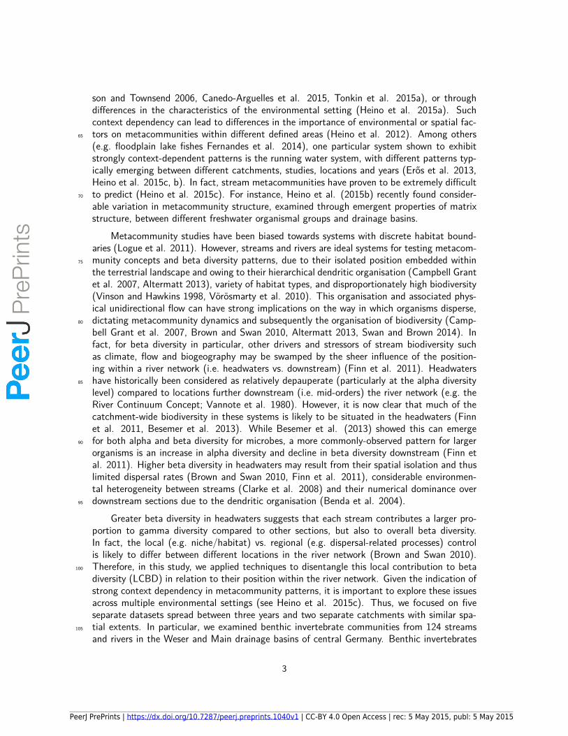
Figure 1: Map of the five datasets, sampled between 2005 and 2007 in the central German state ofHesse. The five datasets are made up of one northern and one southern drainage basin (Weser andMain Rivers, respectively, sampled each year). Insu�cient sites were sampled in 2006 in the northernbasin to be included.

Sites in the two northern datasets (the same general region but sampled in di�erent yearsand di�erent individual sites) were at higher elevation than those in the southern datasets(Tukey’s HSD < 0.05 between all datasets of northern and all southern basins, but not withinthe basins). Catchment size di�erences were less clear, however, with datasets D and E having150

greater catchment sizes than dataset C, and dataset E greater than A (Tukey’s HSD < 0.05).

Sampling

Benthic invertebrates were sampled by German governmental environmental agencies followingthe o�cial EU Water Framework Directive (WFD) compliant sampling protocols for Germanstreams (Haase et al. 2004). This sampling method uses a multi-habitat approach by taking155

20 sample units from each site, based on the proportion of microhabitats present at a site.More specifically, all microhabitats in a 100-m long reach were first recorded in 5% coverageunits, and each sampling unit (25 ◊ 25 cm) sampled with a 0.5-mm mesh kick net. Twentysample units were taken from each site and then pooled for later analysis (1.25 m2 totalsampling area). These microhabitat values were recorded for use in subsequent analyses and160

can be found in Table S2. Collected samples were stored in 70% ethanol and identified in thelaboratory to consistent levels between sites, as proposed by Haase et al. (2006) (i.e. EU-WFD-compliant operational taxon list for German running waters). To partially control formajor anthropogenic stressors, we removed heavily polluted sites using the German saprobityindex. We removed all sites with worse than “medium” saprobity scores.165

5


PrePrin

ts

Environmental variables

In addition to the microhabitat variables (Table S2), catchment land use was calculated for theentire upstream catchment area of each site using data from the CORINE Land Cover database(Bossard et al. 2000). We grouped CORINE classes into seven coarser classes (artificial,agriculture, forest, shrub, natural bare, wetlands, water), but due to low percent coverage of170

some classes, only artificial, agriculture, forest and shrub were kept for our analyses. Thesewere used as explanatory variables in the analyses.

Data analysis

All statistical analyses were carried out in R 3.1.1 (R Core Team 2013).To test the null hypothesis that there was no di�erence in the degree of environmen-175

tal heterogeneity between the five datasets, we tested for homogeneity of group dispersions(PERMDISP2) (Anderson 2006) using the ‘betadisper’ function in the R package vegan (Ok-sanen et al. 2013). This method uses the ANOVA F -statistic to compare the within-groupdistances to each group centroid, and tests for significance between groups using permutation.We tested for di�erences using normalised environmental variables and Euclidean distances.180

Where significant, we compared between individual datasets using pairwise Tukey’s HSD tests.We ran these tests both inclusive and exclusive of catchment size and elevation, to observetheir influence.

As beta diversity should increase with increasing spatial extent (Bini et al. 2014, Heinoet al. 2015d), we also assessed whether there were any di�erences in the spatial extent of185

each dataset using the same approach on geographic coordinates and found no di�erences(F 4,119 = 1.09, P = 0.364).

Multiple approaches to measure beta diversity are often required, depending on the ques-tion of interest, as di�erent measures describe distinct aspects of beta diversity (Anderson etal. 2011). To calculate catchment beta diversity measures, we followed the methods devel-190

oped by Legendre and De Cáceres (2013). We examined overall beta diversity (BD_Total)and local (i.e. individual site-based) contribution to beta diversity (LCBD) using the beta.divfunction, based on the R code provided by Legendre and De Cáceres (2013). We basedour approach on Hellinger-transformed data (i.e. raw abundance data, using the “hellinger”method in “beta.div”). The LCBD metric is essentially an indicator of the uniqueness of each195

site to the entire metacommunity (or, in our case, each dataset).To summarise di�erences between the biodiversity of the five datasets, we compared local

taxonomic richness, Simpson’s diversity index, dataset gamma diversity and total dataset betadiversity (BD_Total). We calculated Simpson’s diversity index (1-D) using the “diversity”function in the R package vegan (Oksanen et al. 2013). We compared mean taxonomic200

richness and Simpson’s diversity index using one-way ANOVAs, followed by pairwise Tukey’sHSD tests, when significant di�erences were observed. Gamma diversity and BD_Total couldnot be compared statistically as they only had one value per dataset.

To test the relationships between catchment size (as a proxy for network position) and

6


PrePrin

ts

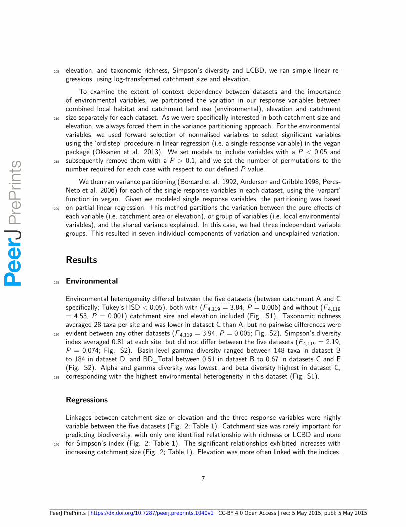
elevation, and taxonomic richness, Simpson’s diversity and LCBD, we ran simple linear re-205

gressions, using log-transformed catchment size and elevation.To examine the extent of context dependency between datasets and the importance

of environmental variables, we partitioned the variation in our response variables betweencombined local habitat and catchment land use (environmental), elevation and catchmentsize separately for each dataset. As we were specifically interested in both catchment size and210

elevation, we always forced them in the variance partitioning approach. For the environmentalvariables, we used forward selection of normalised variables to select significant variablesusing the ‘ordistep’ procedure in linear regression (i.e. a single response variable) in the veganpackage (Oksanen et al. 2013). We set models to include variables with a P < 0.05 andsubsequently remove them with a P > 0.1, and we set the number of permutations to the215

number required for each case with respect to our defined P value.We then ran variance partitioning (Borcard et al. 1992, Anderson and Gribble 1998, Peres-

Neto et al. 2006) for each of the single response variables in each dataset, using the ‘varpart’function in vegan. Given we modeled single response variables, the partitioning was basedon partial linear regression. This method partitions the variation between the pure e�ects of220

each variable (i.e. catchment area or elevation), or group of variables (i.e. local environmentalvariables), and the shared variance explained. In this case, we had three independent variablegroups. This resulted in seven individual components of variation and unexplained variation.

Results

Environmental225

Environmental heterogeneity di�ered between the five datasets (between catchment A and Cspecifically; Tukey’s HSD < 0.05), both with (F 4,119 = 3.84, P = 0.006) and without (F 4,119= 4.53, P = 0.001) catchment size and elevation included (Fig. S1). Taxonomic richnessaveraged 28 taxa per site and was lower in dataset C than A, but no pairwise di�erences wereevident between any other datasets (F 4,119 = 3.94, P = 0.005; Fig. S2). Simpson’s diversity230

index averaged 0.81 at each site, but did not di�er between the five datasets (F 4,119 = 2.19,P = 0.074; Fig. S2). Basin-level gamma diversity ranged between 148 taxa in dataset Bto 184 in dataset D, and BD_Total between 0.51 in dataset B to 0.67 in datasets C and E(Fig. S2). Alpha and gamma diversity was lowest, and beta diversity highest in dataset C,corresponding with the highest environmental heterogeneity in this dataset (Fig. S1).235

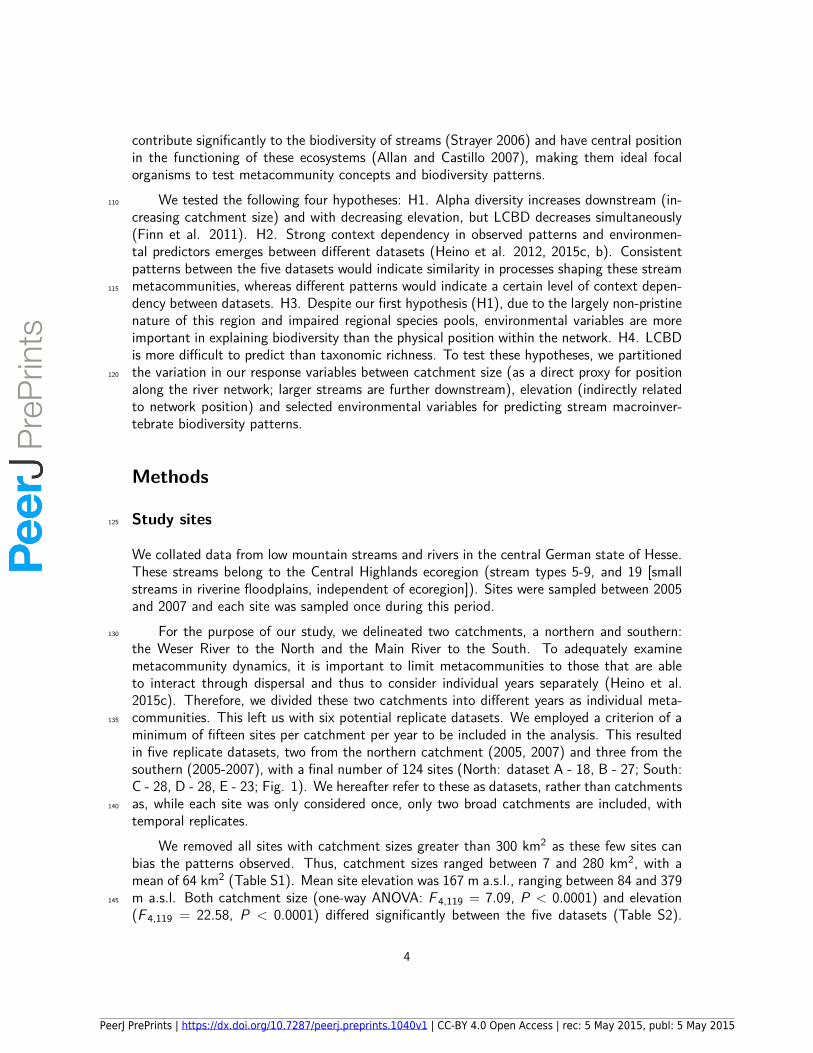
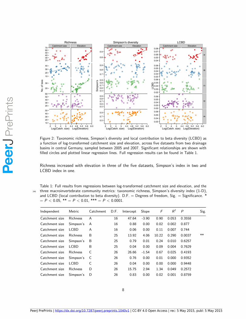
Regressions

Linkages between catchment size or elevation and the three response variables were highlyvariable between the five datasets (Fig. 2; Table 1). Catchment size was rarely important forpredicting biodiversity, with only one identified relationship with richness or LCBD and nonefor Simpson’s index (Fig. 2; Table 1). The significant relationships exhibited increases with240

increasing catchment size (Fig. 2; Table 1). Elevation was more often linked with the indices.

7


PrePrin

ts

Catchment size Elevation

●

●

●

●●

●●●

●

●

●

●●

●

● ●

●●

●

●

●

●

●

●

●

●

●

●

●

●

●

●

●●

●●

●

●

●

●

●●

●

●

●

●

●

●

●●●

●

●

●

●

●● ●

●

●

●

●

●

●

●

●

●

● ●

●●

●●

●

●● ●●● ●

●

● ●●

●

●

●

●

●

●●

●

●

●

●

●●●●

●

●

●

●

●

●●

●

●

●

●

●

●

●

●

●

●●

●

●

●● ●

●●

●

●

●

●●

●●●

●

●

●

●●

●

●●

●●

●

●

●

●

●

●

●

●

●

●

●

●

●

●

●●

●●●

●

●

●

●●

●

●

●

●

●

●

●●●

●

●

●

●

●●●

●

●

●

●

●

●

●

●

●

●●

●●

●●

●

●●● ● ●●

●

●●●

●

●

●

●

●

●●

●

●

●

●

●●●●

●

●

●

●

●

●●

●

●

●

●

●

●

●

●

●

●●

●

●

● ●●

● ●

203040506070

10203040

20

30

2030405060

1020304050

2 3 4 5 4.4 4.8 5.2 5.6 6.0Log(Catch. size) Log(Elevation)

No.

of t

axa

RichnessCatchment size Elevation

●

●

●●

●

●

●●

●●

●

● ●

●

●

●

●

●

●

●

●

●

●

●

●

●

●

●

●

●●

●

● ●

●

● ●

●

●

●

●●●

●

●

●

●

●●

●

●

●

●●

●

●●●

●

●●

●

●

●

●●

●

●

●

●

●●

●

●

●

●

●

●●●

●●

●

●●

●●

●●

●

●

●

●

●

●

●

●

●

●

●

●

●●●●

●

●

●

●●

●

●

●

●

●

●

●

●

●

●●●

●●

●

●

●●

●

●

●●

●●

●

●●

●

●

●

●

●

●

●

●

●

●

●

●

●

●

●

●

●●

●

●●

●

●●

●

●

●

●●●

●

●

●

●

●●●

●

●

●●

●

●●●

●

●●

●

●

●

●●

●

●

●

●

●●

●

●

●

●

●

● ●●

●●

●

●●

●●

●●

●

●

●

●

●

●

●

●

●

●

●

●

●●●●

●

●

●

●●

●

●

●

●

●

●

●

●

●

● ●●

● ●

0.8

0.9

0.7

0.8

0.9

0.50.60.70.80.9

0.50.60.70.80.9

0.5

0.7

0.9

2 3 4 5 4.4 4.8 5.2 5.6 6.0Log(Catch. size) Log(Elevation)

Sim

pson

's

Simpson's diversityCatchment size Elevation

●

●

●

●

●

●

●

●

●

●

●●

●

●

●● ●

●

●

●● ●

●●●

●

●

●

●●

●

●

● ●

●

●

●

●●

●●●

●

●

●

●

●●

●●●

●

●

●

●

●

●

●●

●●

●●● ● ●●●

●

●

●

●

●

● ●

●

●

●●

●●

●●

●

● ●

●

●

●

●

●

●●●

●●●

●

●●

●

●●

●

●● ●●

●

●

●

● ●

●

●

●

●

●

●

●

●

●●

●

●

●

●

●

●

●

●

●

●

●

●●

●

●

●● ●

●

●

●●●

● ●●

●

●

●

●●

●

●

●●

●

●

●

●●

●●●

●

●

●

●

●●

●●●

●

●

●

●

●

●

●●

●●

● ●●●●● ●

●

●

●

●

●

●●

●

●

●●

●●

●●

●

● ●

●

●

●

●

●

●●

●

●●●

●

●●

●

●●

●

● ● ●●

●

●

●

●●

●

●

●

●

●

●

●

●

●●

●

0.040.050.060.070.08

0.020.030.040.050.06

0.020.030.040.050.06

0.020.030.040.050.06

0.030.040.050.06

AB

CD

E

2 3 4 5 4.4 4.8 5.2 5.6 6.0 Log(Catch. size) Log(Elevation)

LCBD

LCBD

Figure 2: Taxonomic richness, Simpson’s diversity and local contribution to beta diversity (LCBD) asa function of log-transformed catchment size and elevation, across five datasets from two drainagebasins in central Germany, sampled between 2005 and 2007. Significant relationships are shown withfilled circles and plotted linear regression lines. Full regression results can be found in Table 1.

Richness increased with elevation in three of the five datasets, Simpson’s index in two andLCBD index in one.

Table 1: Full results from regressions between log-transformed catchment size and elevation, and thethree macroinvertebrate community metrics: taxonomic richness, Simpson’s diversity index (1-D),245

and LCBD (local contribution to beta diversity). D.F. = Degrees of freedom, Sig. = Significance. *= P < 0.05, ** = P < 0.01, *** = P < 0.0001.

Independent Metric Catchment D.F. Intercept Slope F R2 P Sig.

Catchment size Richness A 16 47.64 -3.90 0.90 0.053 0.3558Catchment size Simpson’s A 16 0.88 0.00 0.02 0.002 0.877Catchment size LCBD A 16 0.06 0.00 0.11 0.007 0.744Catchment size Richness B 25 13.92 4.06 10.22 0.290 0.0037 **Catchment size Simpson’s B 25 0.79 0.01 0.24 0.010 0.6257Catchment size LCBD B 25 0.04 0.00 0.09 0.004 0.7629Catchment size Richness C 26 26.66 -1.54 0.67 0.025 0.4193Catchment size Simpson’s C 26 0.76 0.00 0.01 0.000 0.9352Catchment size LCBD C 26 0.04 0.00 0.00 0.000 0.9448Catchment size Richness D 26 15.75 2.94 1.34 0.049 0.2572Catchment size Simpson’s D 26 0.83 0.00 0.02 0.001 0.8759

8


PrePrin

ts

Independent Metric Catchment D.F. Intercept Slope F R2 P Sig.

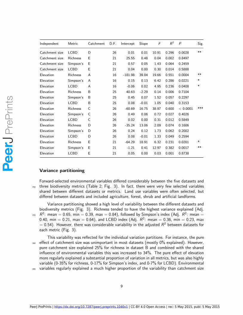
Catchment size LCBD D 26 0.01 0.01 10.91 0.296 0.0028 **Catchment size Richness E 21 25.55 0.48 0.04 0.002 0.8497Catchment size Simpson’s E 21 0.57 0.05 1.43 0.064 0.2459Catchment size LCBD E 21 0.04 0.00 0.30 0.014 0.5888Elevation Richness A 16 -181.98 39.84 19.66 0.551 0.0004 **Elevation Simpson’s A 16 0.15 0.13 6.42 0.286 0.0221 *Elevation LCBD A 16 -0.06 0.02 4.95 0.236 0.0408 *Elevation Richness B 25 40.63 -2.29 0.14 0.006 0.7104Elevation Simpson’s B 25 0.45 0.07 1.52 0.057 0.2297Elevation LCBD B 25 0.08 -0.01 1.05 0.040 0.3153Elevation Richness C 26 -60.69 16.75 38.97 0.600 < 0.0001 ***Elevation Simpson’s C 26 0.49 0.06 0.72 0.027 0.4026Elevation LCBD C 26 0.02 0.00 0.31 0.012 0.5849Elevation Richness D 26 -35.24 13.06 2.09 0.074 0.1606Elevation Simpson’s D 26 0.24 0.12 1.73 0.062 0.2002Elevation LCBD D 26 0.08 -0.01 1.33 0.049 0.2594Elevation Richness E 21 -64.29 18.91 6.32 0.231 0.0201 *Elevation Simpson’s E 21 -1.21 0.41 12.97 0.382 0.0017 **Elevation LCBD E 21 0.05 0.00 0.03 0.001 0.8738

Variance partitioning

Forward-selected environmental variables di�ered considerably between the five datasets andthree biodiversity metrics (Table 2; Fig. 3). In fact, there were very few selected variables250

shared between di�erent datasets or metrics. Land use variables were often selected, butdi�ered between datasets and included agriculture, forest, shrub and artificial landforms.

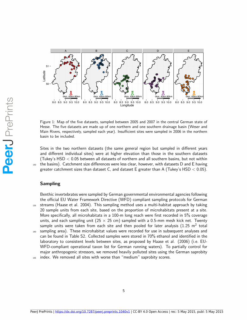
Variance partitioning showed a high level of variability between the di�erent datasets andbiodiversity metrics (Fig. 3). Richness tended to have the highest variance explained (Adj.R2: mean = 0.65, min = 0.39, max = 0.84), followed by Simpson’s index (Adj. R2: mean =255

0.40, min = 0.21, max = 0.64), and LCBD index (Adj. R2: mean = 0.36, min = 0.23, max= 0.54). However, there was considerable variability in the adjusted R2 between datasets foreach metric (Fig. 3).

This variability was reflected for the individual variation partitions. For instance, the puree�ect of catchment size was unimportant in most datasets (mostly 0% explained). However,260

pure catchment size explained 25% for richness in dataset B and combined with the sharedinfluence of environmental variables this was increased to 34%. The pure e�ect of elevationmore regularly explained a substantial proportion of variation in all metrics, but was also highlyvariable (0-35% for richness, 0-17% for Simpson’s index, and 0-7% for LCBD). Environmentalvariables regularly explained a much higher proportion of the variability than catchment size265

9


PrePrin

ts

Richness Simpson's LCBD

0.04 0.26

0.11

0.01

0.28

0.35(Resid.)

0.25

0.09

0

0.040.09

0.61(Resid.)

0.35

0.02

0.2500

0.4(Resid.)

0.02

0.74

0

0.020.02

0.21(Resid.)

0.68

0

0.2

0.16(Resid.)

0.43

0.01

0.27

0.38(Resid.)

0.01 0.01

0.23

0.080.03

0.71(Resid.)

0.26

0.01

0.79(Resid.)

0.01

0.25

0.050

0.76(Resid.)

0 0.17

0.26

0.190.020.01

0.36(Resid.)

0.07

0.13

0

0.12

0.73(Resid.)

0.27

0.010.01

0.77(Resid.)

0.35

0.01

0.71(Resid.)

0

0.24

0.040.28

0.46(Resid.)

0 0.04

0.55

0.01

0.53(Resid.)

AB

CD

E

Partition ● ● ●Catchment Elevation Environmental

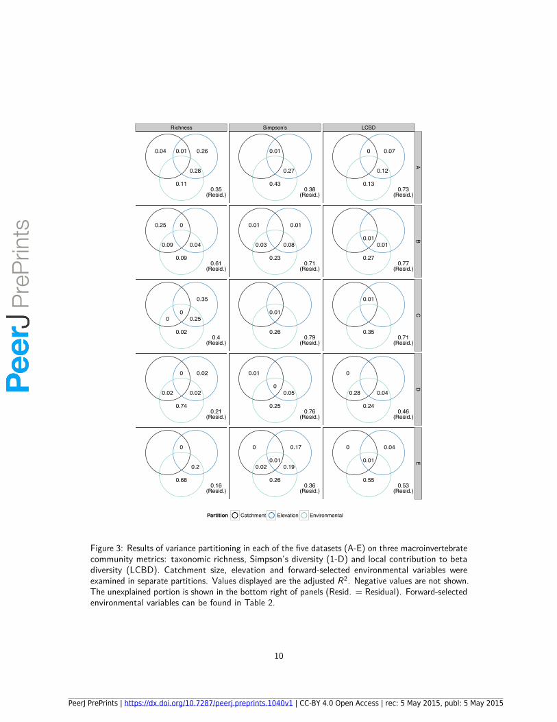
Figure 3: Results of variance partitioning in each of the five datasets (A-E) on three macroinvertebratecommunity metrics: taxonomic richness, Simpson’s diversity (1-D) and local contribution to betadiversity (LCBD). Catchment size, elevation and forward-selected environmental variables wereexamined in separate partitions. Values displayed are the adjusted R2. Negative values are not shown.The unexplained portion is shown in the bottom right of panels (Resid. = Residual). Forward-selectedenvironmental variables can be found in Table 2.

10


PrePrin

ts

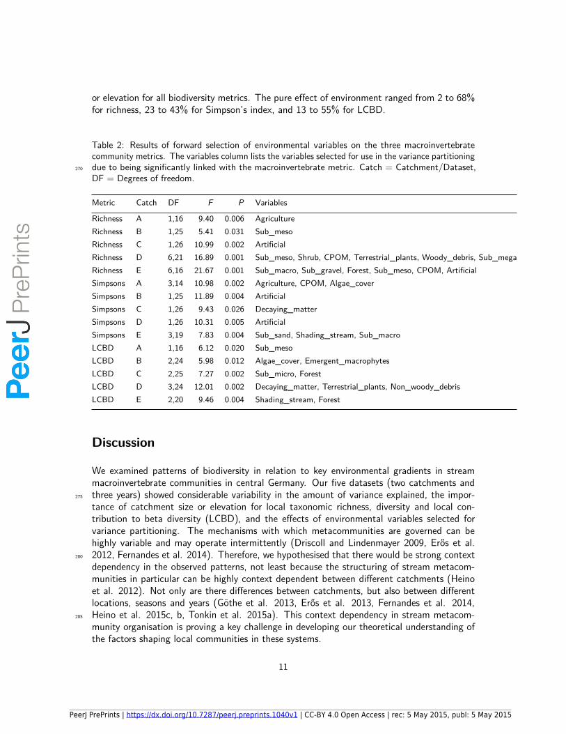
or elevation for all biodiversity metrics. The pure e�ect of environment ranged from 2 to 68%for richness, 23 to 43% for Simpson’s index, and 13 to 55% for LCBD.

Table 2: Results of forward selection of environmental variables on the three macroinvertebratecommunity metrics. The variables column lists the variables selected for use in the variance partitioningdue to being significantly linked with the macroinvertebrate metric. Catch = Catchment/Dataset,270

DF = Degrees of freedom.

Metric Catch DF F P Variables

Richness A 1,16 9.40 0.006 AgricultureRichness B 1,25 5.41 0.031 Sub_mesoRichness C 1,26 10.99 0.002 ArtificialRichness D 6,21 16.89 0.001 Sub_meso, Shrub, CPOM, Terrestrial_plants, Woody_debris, Sub_megaRichness E 6,16 21.67 0.001 Sub_macro, Sub_gravel, Forest, Sub_meso, CPOM, ArtificialSimpsons A 3,14 10.98 0.002 Agriculture, CPOM, Algae_coverSimpsons B 1,25 11.89 0.004 ArtificialSimpsons C 1,26 9.43 0.026 Decaying_matterSimpsons D 1,26 10.31 0.005 ArtificialSimpsons E 3,19 7.83 0.004 Sub_sand, Shading_stream, Sub_macroLCBD A 1,16 6.12 0.020 Sub_mesoLCBD B 2,24 5.98 0.012 Algae_cover, Emergent_macrophytesLCBD C 2,25 7.27 0.002 Sub_micro, ForestLCBD D 3,24 12.01 0.002 Decaying_matter, Terrestrial_plants, Non_woody_debrisLCBD E 2,20 9.46 0.004 Shading_stream, Forest

Discussion

We examined patterns of biodiversity in relation to key environmental gradients in streammacroinvertebrate communities in central Germany. Our five datasets (two catchments andthree years) showed considerable variability in the amount of variance explained, the impor-275

tance of catchment size or elevation for local taxonomic richness, diversity and local con-tribution to beta diversity (LCBD), and the e�ects of environmental variables selected forvariance partitioning. The mechanisms with which metacommunities are governed can behighly variable and may operate intermittently (Driscoll and Lindenmayer 2009, Er�s et al.2012, Fernandes et al. 2014). Therefore, we hypothesised that there would be strong context280

dependency in the observed patterns, not least because the structuring of stream metacom-munities in particular can be highly context dependent between di�erent catchments (Heinoet al. 2012). Not only are there di�erences between catchments, but also between di�erentlocations, seasons and years (Göthe et al. 2013, Er�s et al. 2013, Fernandes et al. 2014,Heino et al. 2015c, b, Tonkin et al. 2015a). This context dependency in stream metacom-285

munity organisation is proving a key challenge in developing our theoretical understanding ofthe factors shaping local communities in these systems.

11


PrePrin

ts

The selected environmental variables tended to explain a greater proportion of the vari-ation in biodiversity metrics than either catchment size or elevation in these datasets. Thismay reflect the largely impaired nature of these ecosystems. This finding contrasts with the290

suggestion of Finn et al. (2011) that the positioning within a river network (i.e. headwatersvs. downstream) may override other factors (including stressors) shaping stream biodiversity,such as climate, flow and biogeography. The importance of neutral processes relating to rivernetwork structure have been clearly demonstrated. For instance, Muneepeerakul et al. (2008)predicted fish biodiversity patterns in the Mississippi-Missouri River System using a neutral295

metacommunity model that included spatial and dispersal factors alone, which has been sup-ported using experimental systems (Carrara et al. 2012). Stream studies in relatively pristineregions also show clearly context-dependent patterns in associations between environment,space and biological communities (e.g. Heino et al. 2012). Streams are highly stochasticsystems, with strong fluctuations in environmental conditions, particularly the flow regime300

(Resh et al. 1988) with its associated substrate disturbance (Tonkin and Death 2012). Asa result, observed metacommunity patterns can fluctuate temporally in these systems (Götheet al. 2013, Er�s et al. 2013). A recent study focusing on partitioning environmental andspatial control demonstrated that stream metacommunities di�er depending on the precedingflow conditions (Campbell et al. 2015). This represents a key issue with one-o� sampling, as305

species that are present one year due to favourable preceding conditions can be missed thefollowing year (Er�s et al. 2013, Andersson et al. 2014). Moreover, a potentially greateramount of variation might have been captured if we had incorporated chemical stressors inour analysis, but consistent data for these sites was unfortunately unavailable. Despite thelack of such variables, we were able to explain a sizeable portion of variation in our response310

variables using the measured environmental variables.Overall beta diversity was linked with regional environmental heterogeneity (Fig. S1,

Fig. S2), which reflects a greater availability of niches, and is consistent with many findings(see Heino et al. 2015d). Nevertheless, greater gamma diversity did not emerge in moreheterogeneous regions. Beta diversity can be promoted through a suite of di�erent processes,315

including dispersal limitation (Shurin et al. 2009), environmental heterogeneity (Heino et al.2015d), productivity (Bini et al. 2014), and spatial extent (Heino et al. 2015e). While it iswell understood that communities are formed through an interplay between local and regionalprocesses (Leibold et al. 2004), we focused on local habitat conditions and catchment landuse to explain biodiversity patterns in our study, which captured a substantial proportion of the320

variability in biodiversity. The balance between local and regional processes may di�er betweendi�erent locations in the river network (Brown and Swan 2010), and we thus incorporatedelevation and catchment size as proxies for network position. While the relationship is likelyscale dependent, within-stream habitat heterogeneity may in some cases be more importantthan regional- or landscape-scale factors in determining beta diversity of stream invertebrates325

(Astorga et al. 2014). Local habitat conditions have been clearly demonstrated as a key factordetermining stream invertebrate communities in pristine streams (Heino et al. 2012, Tonkin2014), and the importance of land use in shaping stream communities is well understood(e.g. Harding et al. 1998). In fact, local variables may override regional processes on streammetacommunities, where there is substantial heterogeneity in conditions across space and330

time (Canedo-Arguelles et al. 2015) and if dispersal processes do not interfere with speciessorting (Heino et al. 2015d). Nevertheless, we predicted a decrease in beta diversity from

12


PrePrin

ts

headwaters downstream as, although streams are highly heterogeneous systems with strongdi�erences even between di�erent ri�es, this heterogeneity in both habitat and biota is likelyto decrease downstream (Heino et al. 2004, Finn et al. 2011).335

In line with our hypothesis, our predictor variables were unable to explain as much variationin LCBD as for taxonomic richness or diversity. LCBD essentially represents the uniquenessof a community in relation to other communities within a metacommunity (Legendre andDe Cáceres 2013), and high values thus represent sites with highly unique communities.This of course can be used to identify sites with high conservation value (or restoration340

potential in the case of species poor communities), those with invasive species, or those withunique environmental conditions (Legendre and De Cáceres 2013). The poor link betweenenvironment and LCBD in our study potentially emerged through impacted species poolsin this region, through a long history of anthropogenic modification. Göthe et al. (2015)came to a similar conclusion in a recent study on biodiversity patterns in streams of a region345

with a long history of anthropogenic modification. Recent studies have clearly highlightedthe importance of intact species pools for restoration to succeed (Sundermann et al. 2011,Tonkin et al. 2014), but also that anthropogenic degradation can alter associations betweendi�erent species in streams (Larsen and Ormerod 2014, Tonkin et al. 2015b). Nevertheless,the poor prediction of LCBD may also simply reflect the fact that it is a di�cult metric to350

explain, and the evidence is currently scarce as this metric is a relatively new measure of betadiversity (but see e.g. Silva and Hernández 2014, Lopes et al. 2014). Furthermore, streammetacommunities can be notoriously di�cult to predict, as evidenced by a recent global studythat showed weak and variable patterns in the factors shaping beta diversity and communitystructure (Heino et al. 2015c).355

Physical isolation is a key factor governing metacommunity dynamics (Driscoll and Lin-denmayer 2009). Thus, we hypothesised that LCBD would decline downstream (i.e. withincreasing catchment size), and alpha diversity would increase simultaneously. Substantialevidence exists that although headwaters may have lower alpha diversity (but see Besemer etal. 2013), they contribute substantially to overall gamma diversity through high site-to-site360

variation between streams (beta diversity) (e.g. Finn et al. 2011). Yet, we found no evidenceto support this, with the only trend for LCBD being an increase downstream (i.e. with in-creasing catchment size) in one dataset. Göthe et al. (2015) also recently found no evidenceof higher beta diversity in headwater streams in a degraded landscape. Higher beta diversityin headwaters is thought to emerge for a variety of reasons, including shorter environmental365

gradients, and greater isolation and thus more influential dispersal limitation. These patternsmay be reflecting the dispersal abilities of stream invertebrates, potentially overriding nichecontrol through overcoming geographic barriers. However, the extent of interchange betweenheadwater branches remains unclear and is likely species specific (Hughes 2007, Geismar et al.2015). Headwaters are also thought to harbour more habitat specialists (Meyer et al. 2007),370

which again should contribute to higher individual contributions to beta and gamma diversity.While environmental control may be greater in headwaters (Brown and Swan 2010, Göthe etal. 2013), as in most systems, headwater communities are governed by an interplay betweenlocal and regional (species pool) factors (Heino et al. 2003, Grönroos and Heino 2012). Nev-ertheless, catchment size was a poor predictor in our study in general, with more regular and375

clearer links found with elevation. Where a significant relationship between the two networklocation variables (i.e. catchment size and elevation) and biodiversity was present, biodiversity

13


PrePrin

ts

always increased.One possible reason for a lack of association with catchment size is an uneven repre-

sentation of sites along the full environmental gradient in our datasets (i.e. small headwater380

streams were underrepresented). However, while we had few streams of first order size, 41sites in total had catchment sizes of less than 20 km2 (all datasets had at least four sitessmaller than this). Nevertheless, we believe we covered an adequate gradient to exert clearpatterns along the river size gradient (from 7 to 280 km2). At the heart of the RCC was theidea that environmental conditions change predictably downstream and lead to biodiversity385

peaking in mid-order streams through greater environmental heterogeneity, with headwatersbeing relatively depauperate (Vannote et al. 1980). Our results cannot refute this suggestion,but it may be that external stressors are influencing the context-dependent patterns in oursystem. The strong increase in biodiversity variables with elevation in a lot of cases maysuggest better environmental conditions are available at higher elevations and that increas-390

ing stressors emerge in downstream sites. Nevertheless, we would still expect to see greaterbeta diversity at smaller catchment sizes and with increasing elevation. The promotion ofbeta diversity in isolated positions within dendritic networks is well supported, for instancein experimental protist metacommunities (Carrara et al. 2012), and in field data of streaminvertebrate communities (Finn et al. 2011).395

River networks and other dendritic systems are unique systems for examining the pro-cesses shaping metacommunities. One of the key findings to emerge through consideringrivers systems from a network perspective is the knowledge that headwaters are critical biodi-versity reservoirs. However, we found no evidence to support this in our study, with no declinein LCBD downstream, and a much stronger role of local habitat and catchment land use400

variables than catchment size and elevation (proxies of network position). We found highlycontext-dependent patterns between di�erent datasets in our study. Context dependency isa clear challenge for the study of metacommunities, making extrapolation of findings beyondindividual studies di�cult and thus posing a key obstacle to overcome for the developmentof general ecological theories. Therefore, we urge researchers to continue focusing on disen-405

tangling the primary drivers of this variability between metacommunities through studies onreplicate, rather than singular, metacommunities.

Acknowledgements

This study was partly financed by the research funding program LOEWE (Landes-O�ensivezur Entwicklung Wissenschaftlich-oekonomischer Exzellenz) of Hesse’s Ministry of Higher Ed-410

ucation, Research, and the Arts. All data were kindly provided by the Hessisches Landesamtfür Umwelt und Geologie (HLUG), which is greatly acknowledged. JH was supported by theAcademy of Finland. SCJ acknowledges funding by the German Federal Ministry of Educationand Research (BMBF) for “GLANCE” (Global change e�ects in river ecosystems; referencenumber 01LN1320A).415

14


PrePrin

ts

References

Allan, J. D. and Castillo, M. M. 2007. Stream Ecology: Structure and Function of RunningWaters. - Chapman; Hall, London.

Altermatt, F. 2013. Diversity in riverine metacommunities: a network perspective. - AquaticEcology 47: 365–377.420

Anderson, M. J. 2006. Distance-based tests for homogeneity of multivariate dispersions. -Biometrics 62: 245–253.

Anderson, M. J. and Gribble, N. A. 1998. Partitioning the variation among spatial, temporaland environmental components in a multivariate data set. - Australian Journal of Ecology23: 158–167.425

Anderson, M. J. et al. 2011. Navigating the multiple meanings of — diversity: a roadmap forthe practicing ecologist. - Ecology Letters 14: 19–28.

Andersson, M. G. I. et al. 2014. The spatial structure of bacterial communities is influencedby historical environmental conditions. - Ecology 95: 1134–1140.

Angeler, D. G. and Drakare, S. 2013. Tracing alpha, beta, and gamma diversity responses to430

environmental change in boreal lakes. - Oecologia 172: 1191–1202.Astorga, A. et al. 2014. Habitat heterogeneity drives the geographical distribution of beta

diversity: the case of New Zealand stream invertebrates. - Ecology and Evolution 4:2693–702.

Benda, L. et al. 2004. The network dynamics hypothesis: How channel networks structure435

riverine habitats. - Bioscience 54: 413–427.Besemer, K. et al. 2013. Headwaters are critical reservoirs of microbial diversity for fluvial

networks. - Proceedings of The Royal Society B 280: 20131760.Bini, L. et al. 2014. Nutrient enrichment is related to two facets of beta diversity of stream

invertebrates across the continental US. - Ecology 95: 1569–1578.440

Borcard, D. et al. 1992. Partialling out the spatial component of ecological variation. -Ecology 73: 1045–1055.

Bossard, M. et al. 2000. CORINE land cover technical guide – Addendum 2000.: 105.Brown, B. L. and Swan, C. M. 2010. Dendritic network structure constrains metacommunity

properties in riverine ecosystems. - Journal of Animal Ecology 79: 571–580.445

Campbell, R. E. et al. 2015. Flow-related disturbance creates a gradient of metacommunitytypes within stream networks. - Landscape Ecology: DOI:10.1007/s10980–015–0164–x.

Campbell Grant, E. H. et al. 2007. Living in the branches: population dynamics and ecologicalprocesses in dendritic networks. - Ecology Letters 10: 165–175.Canedo-Arguelles, M. et al. 2015. Dispersal strength determines meta-community structure450

in a dendritic riverine network. - Journal of Biogeography: 1–13.

15


PrePrin

ts

Carrara, F. et al. 2012. Dendritic connectivity controls biodiversity patterns in experimentalmetacommunities. - Proceedings of the National Academy of Sciences of the UnitedStates of America 109: 5761–5766.

Clarke, A. et al. 2008. Macroinvertebrate diversity in headwater streams: a review. -455

Freshwater Biology 53: 1707–1721.Driscoll, D. and Lindenmayer, D. B. 2009. Empirical tests of metacommunity theory using an

isolation gradient. - Ecological Monographs 79: 485–501.Dudgeon, D. et al. 2006. Freshwater biodiversity: importance, threats, status and con-

servation challenges. - Biological reviews of the Cambridge Philosophical Society 81:460

163–182.Er�s, T. et al. 2012. Temporal variability in the spatial and environmental determinants of

functional metacommunity organization - stream fish in a human-modified landscape. -Freshwater Biology 57: 1914–1928.

Er�s, T. et al. 2013. Quantifying temporal variability in the metacommunity structure of465

stream fishes: the influence of non-native species and environmental drivers. - Hydrobi-ologia 722: 31–43.

Fernandes, I. M. et al. 2014. Spatiotemporal dynamics in a seasonal metacommunity structureis predictable: the case of floodplain-fish communities. - Ecography 37: 464–475.

Finn, D. S. et al. 2011. Small but mighty: headwaters are vital to stream network biodiversity470

at two levels of organization. - Journal of the North American Benthological Society 30:963–980.

Geismar, J. et al. 2015. Local population genetic structure of the montane caddisfly Drususdiscolor is driven by overland dispersal and spatial scaling. - Freshwater Biology 60:209–221.475

Göthe, E. et al. 2013. Metacommunity structure in a small boreal stream network. - Journalof Animal Ecology 82: 449–58.

Göthe, E. et al. 2015. Impacts of habitat degradation and stream spatial location onbiodiversity in a disturbed riverine landscape. - Biodiversity and Conservation: DOI:10.1007/s10531–015–0865–0.480

Grönroos, M. and Heino, J. 2012. Species richness at the guild level: E�ects of species pooland local environmental conditions on stream macroinvertebrate communities. - Journalof Animal Ecology 81: 679–691.

Haase, P. et al. 2004. Assessing streams in Germany with benthic invertebrates: develop-ment of a practical standardised protocol for macroinvertebrate sampling and sorting. -485

Limnologica 34: 349–365.Haase, P. et al. 2006. Informationstext zur Operationellen Taxaliste als Mindestanforderung

an die Bestimmung von Makrozoobenthosproben aus Fliebgewässern zur Umsetzung derEU-Wasserrahmenrichtlinie in Deutschland. - Fliessgewaesserbewertung, Essen, Ger-many.490

16


PrePrin

ts

Harding, J. S. et al. 1998. Stream biodiversity: The ghost of land use past. - Proceedings ofthe National Academy of Sciences 95: 14843–14847.

Heino, J. et al. 2003. Determinants of macroinvertebrate diversity in headwater streams:regional and local influences. - Journal of Animal Ecology 72: 425–434.

Heino, J. et al. 2004. Identifying the scales of variability in stream macroinvertebrate abun-495

dance, functional composition and assemblage structure. - Freshwater Biology 49: 1230–1239.

Heino, J. et al. 2012. Context dependency and metacommunity structuring in boreal head-water streams. - Oikos 121: 537–544.

Heino, J. et al. 2015a. Elements of metacommunity structure and community- environment500

relationships in stream organisms. - Freshwater Biology: DOI:10.1111/fwb.12556.Heino, J. et al. 2015b. A comparative analysis of metacommunity types in the freshwater

realm. - Ecology and Evolution: DOI:10.1002/ece3.1460.Heino, J. et al. 2015c. A comparative analysis reveals weak relationships between ecological

factors and beta diversity of stream insect metacommunities at two spatial levels. -505

Ecology and Evolution 5: 1235–1248.Heino, J. et al. 2015d. Reconceptualising the beta diversity-environmental heterogeneity

relationship in running water systems. - Freshwater Biology 60: 223–235.Heino, J. et al. 2015e. Metacommunity organisation, spatial extent and dispersal

in aquatic systems: patterns, processes and prospects. - Freshwater Biology:510

DOI:10.1111/fwb.12533.Holyoak, M. et al. 2005. Metacommunities: Spatial Dynamics and Ecological Communities.

- University of Chicago Press.Hughes, J. M. 2007. Constraints on recovery: Using molecular methods to study connectivity

of aquatic biota in rivers and streams. - Freshwater Biology 52: 616–631.515

Jackson, D. A. et al. 2001. What controls who is where in freshwater fish communities - theroles of biotic, abiotic, and spatial factors. - Canadian Journal of Fisheries and AquaticSciences 58: 157–170.

Larsen, S. and Ormerod, S. J. 2014. Anthropogenic modification disrupts species co-occurrence in stream invertebrates. - Global Change Biology 20: 51–60.520

Legendre, P. and De Cáceres, M. 2013. Beta diversity as the variance of community data:dissimilarity coe�cients and partitioning. - Ecology letters 16: 951–63.

Leibold, M. A. et al. 2004. The metacommunity concept: a framework for multi-scalecommunity ecology. - Ecology Letters 7: 601–613.

Logue, J. B. et al. 2011. Empirical approaches to metacommunities: a review and comparison525

with theory. - Trends in Ecology & Evolution 26: 482–491.Lopes, P. M. et al. 2014. Correlates of Zooplankton Beta Diversity in Tropical Lake Systems.

- PloS one 9: e109581.

17


PrePrin

ts

Meyer, J. L. et al. 2007. The contribution of headwater streams to biodiversity in rivernetworks. - Journal of the American Water Resources association 43: 86–103.530

Muneepeerakul, R. et al. 2008. Neutral metacommunity models predict fish diversity patternsin Mississippi-Missouri basin. - Nature 453: 220–222.

Oksanen, J. et al. 2013. Vegan: Community Ecology Package. R package version 2.0-10.:http://CRAN.R–project.org/package=vegan.

Peres-Neto, P. et al. 2006. Variation partitioning of species data matrices: estimation and535

comparison of fractions. - Ecology 87: 2614–2625.R Core Team 2013. R: A language and environment for statistical computing.Resh, V. H. et al. 1988. The role of disturbance in stream ecology. - Journal of the North

American Benthological Society 7: 433–455.Shurin, J. B. et al. 2009. Spatial autocorrelation and dispersal limitation in freshwater540

organisms. - Oecologia 159: 151–159.Silva, P. G. D. and Hernández, M. I. M. 2014. Local and Regional E�ects on Community

Structure of Dung Beetles in a Mainland-Island Scenario. - PLoS ONE 9: e111883.Strayer, D. L. 2006. Challenges for freshwater invertebrate conservation. - Journal of the

North American Benthological Society 25: 271–287.545

Sundermann, A. et al. 2011. River restoration success depends on the species pool of theimmediate surroundings. - Ecological Applications 21: 1962–71.

Swan, C. M. and Brown, B. L. 2014. Using rarity to infer how dendritic network structureshapes biodiversity in riverine communities. - Ecography: DOI:10.1111/ecog.00496.

Thompson, R. and Townsend, C. 2006. A truce with neutral theory: local deterministic550

factors, species traits and dispersal limitation together determine patterns of diversity instream invertebrates. - Journal of Animal Ecology 75: 476–484.

Tonkin, J. D. 2014. Drivers of macroinvertebrate community structure in unmodified streams.- PeerJ 2: e465.

Tonkin, J. and Death, R. 2012. Consistent e�ects of productivity and disturbance on diversity555

between landscapes. - Ecosphere 3: art108.Tonkin, J. D. et al. 2014. Dispersal distance and the pool of taxa, but not barriers, determine

the colonisation of restored river reaches by benthic invertebrates. - Freshwater Biology59: 1843–1855.

Tonkin, J. D. et al. 2015a. Variable elements of metacommunity structure across an aquatic-560

terrestrial ecotone. - PeerJ PrePrints 3: e1261.Tonkin, J. D. et al. 2015b. Anthropogenic stress alters community concordance at the

river-riparian interface. - PeerJ PrePrints 3: e798v1.Vannote, R. L. et al. 1980. The river continuum concept. - Canadian Journal of Fisheries

and Aquatic Sciences 37: 130–137.565

18


PrePrin

ts

Vinson, M. R. and Hawkins, C. P. 1998. Biodiversity of stream insects: variation at local,basin, and regional scales. - Annual Review of Entomology 43: 271–293.

Vörösmarty, C. J. et al. 2010. Global threats to human water security and river biodiversity.- Nature 467: 555–561.

Whittaker, R. H. 1960. Vegetation of the Siskiyou mountains, Oregon and California. -570

Ecological Monographs 30: 279–338.

19


PrePrin

ts

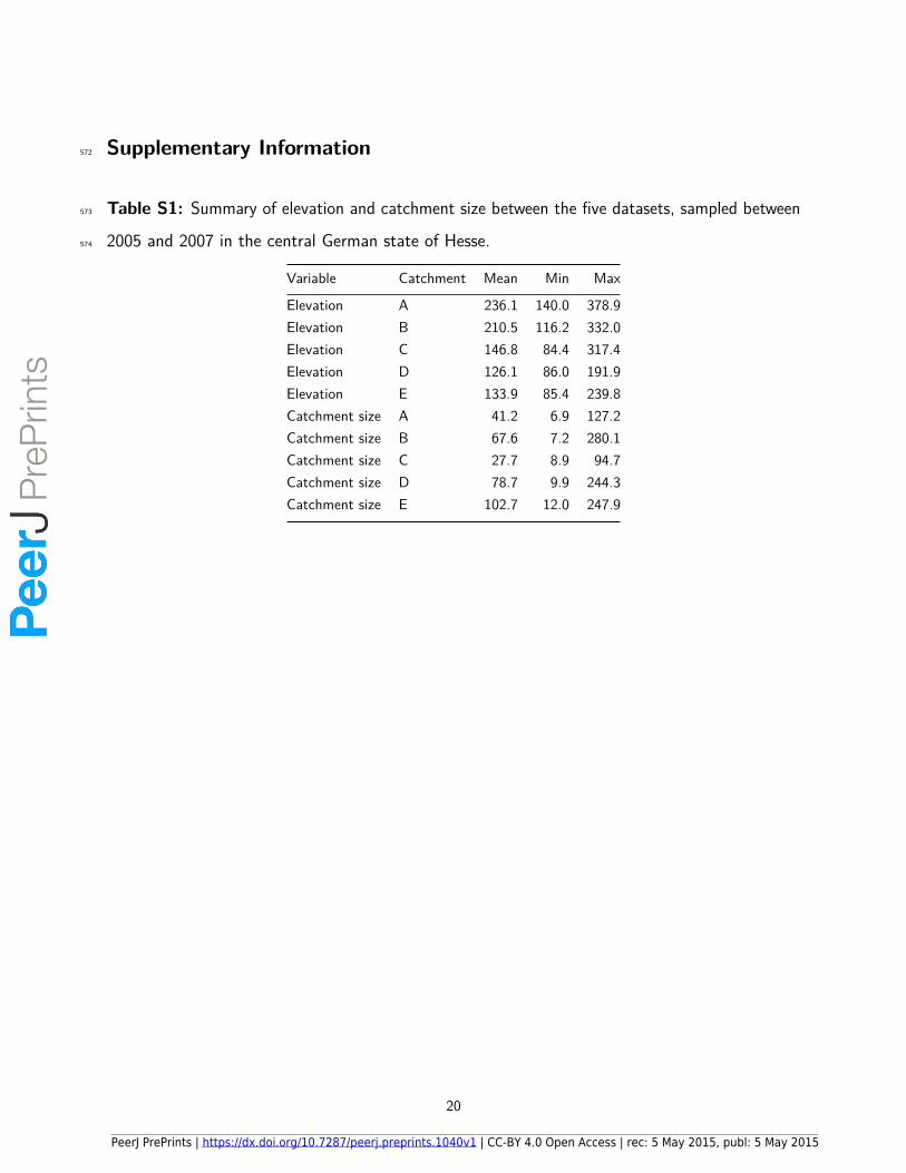
Supplementary Information572

Table S1: Summary of elevation and catchment size between the five datasets, sampled between573

2005 and 2007 in the central German state of Hesse.574

Variable Catchment Mean Min Max

Elevation A 236.1 140.0 378.9Elevation B 210.5 116.2 332.0Elevation C 146.8 84.4 317.4Elevation D 126.1 86.0 191.9Elevation E 133.9 85.4 239.8Catchment size A 41.2 6.9 127.2Catchment size B 67.6 7.2 280.1Catchment size C 27.7 8.9 94.7Catchment size D 78.7 9.9 244.3Catchment size E 102.7 12.0 247.9

20


PrePrin

ts

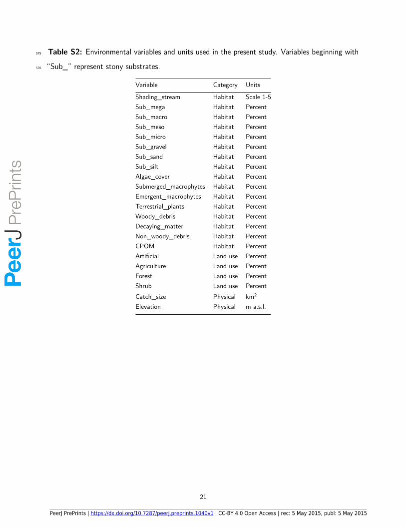
Table S2: Environmental variables and units used in the present study. Variables beginning with575

“Sub_” represent stony substrates.576

Variable Category Units

Shading_stream Habitat Scale 1-5Sub_mega Habitat PercentSub_macro Habitat PercentSub_meso Habitat PercentSub_micro Habitat PercentSub_gravel Habitat PercentSub_sand Habitat PercentSub_silt Habitat PercentAlgae_cover Habitat PercentSubmerged_macrophytes Habitat PercentEmergent_macrophytes Habitat PercentTerrestrial_plants Habitat PercentWoody_debris Habitat PercentDecaying_matter Habitat PercentNon_woody_debris Habitat PercentCPOM Habitat PercentArtificial Land use PercentAgriculture Land use PercentForest Land use PercentShrub Land use PercentCatch_size Physical km2

Elevation Physical m a.s.l.

21


PrePrin

ts

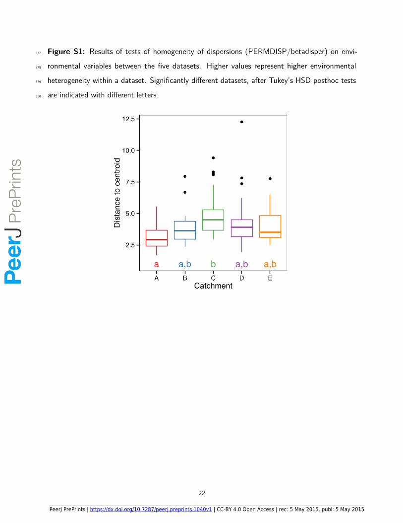
Figure S1: Results of tests of homogeneity of dispersions (PERMDISP/betadisper) on envi-577

ronmental variables between the five datasets. Higher values represent higher environmental578

heterogeneity within a dataset. Significantly di�erent datasets, after Tukey’s HSD posthoc tests579

are indicated with di�erent letters.580

●

●

●●

●

●●

●

●

●

a a,b b a,b a,b

2.5

5.0

7.5

10.0

12.5

A B C D ECatchment

Dis

tanc

e to

cen

troid

22


PrePrin

ts

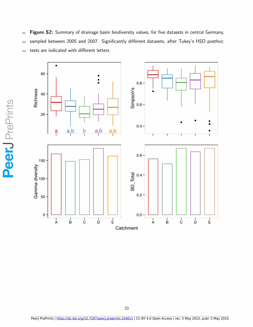
Figure S2: Summary of drainage basin biodiversity values, for five datasets in central Germany,581

sampled between 2005 and 2007. Significantly di�erent datasets, after Tukey’s HSD posthoc582

tests are indicated with di�erent letters.583

●

●

●

●

a a,b b a,b a,b

20

40

60

Ric

hnes

s

●

●● ●

●

●0.4

0.6

0.8

Sim

pson

's

0

50

100

150

A B C D E

Gam

ma

dive

rsity

0.0

0.2

0.4

0.6

A B C D E

BD_T

otal

Catchment

23


PrePrin

ts

Documents

Context dependency in biodiversity patterns of stream