Embed Size (px)
Citation preview
UNIVERSITY OF CALIFORNIA, SAN DIEGO
Continuous Measurements of Atmospheric Ar/N2 as a Tracer of
Air-Sea Heat Flux: Models, Methods, and Data
A dissertation submitted in partial satisfaction of the
requirements for the degree Doctor of Philosophy in
Oceanography
by
Tegan Woodward Blaine
Committee in charge:
Professor Ralph F. Keeling, Chair Professor Paul Robbins Professor Jeff Severinghaus Professor Richard Somerville Professor Mark Thiemens Professor Ray Weiss
2005

Copyright
Tegan Woodward Blaine, 2005
All rights reserved.

iii
The dissertation of Tegan Woodward Blaine is approved, and it is acceptable in quality and form for publication on microfilm:
Chair
University of California, San Diego
2005
iv
TABLE OF CONTENTS Signature Page ……………………………………… iii
Table of Contents …………………………………... iv
List of Figures and Tables ………………………….. vii
Acknowledgements ………………………………… x
Vita and Publications ………………………………. xiii
Abstract …………………………………………….. xiv Chapter 1. Introduction ………………………………………… 1 1.1 Background ……………………………………. 1 1.2 Atmospheric geochemistry ……………………. 9 1.3 Overview of research …………………………. 12 1.4 Bibliography ………………………………….. 16 Chapter 2. Testing tracer transport models with combined measurements of atmospheric O2 and CO2 ………… 22 2.1 Introduction ……………………………………. 22 2.2 Methods ………………………………………... 28 2.2.1 Surface O2 and N2 fluxes ……………….. 28 2.2.2 Submitted model output ………………… 30 2.2.3 Model descriptions ……………………… 31 2.3 Results …………………………………………. 34 2.3.1 Comparison of station measurements and model predictions ………………….. 34 2.3.2 Station-station comparisons …………….. 42 2.3.3 Global surface patterns …………………. 49 2.3.4 Zonal patterns ….……………………….. 53
2.3.5 Transects of amplitude, rectifier, and phase along 60o North and South ……..... 60 2.4 Discussion ……………………………………... 63 2.5 Conclusions ……………………………………. 67 2.6 Bibliography …………………………………… 69 Chapter 3. Air-sea heat flux and the related seasonal cycle of δ(Ar/N2) …………………………………… 74 3.1 Introduction ……………………………………. 74
v
3.2 The seasonal cycle in δ(Ar/N2): A transient model of air-sea gas flux ……………………… 78 3.3 A note on latitudinal gradients ………………… 93 3.4 Global maps of the expected seasonal cycle in surface δ(Ar/N2) …………………………….. 99 3.5 Conclusions ……………………………………. 101 3.6 Bibliography ..…………………………………. 103 Chapter 4. Development of a continuous method for determining atmospheric δ(Ar/N2) ………………… 107 4.1 Introduction ……………………………………. 107 4.2 Instrument description …………………………. 109 4.3 Calibration ……………………………………... 119 4.3.1 Establishing ion sensitivities ……………. 119 4.3.2 Long-term stability of reference gases ….. 123 4.4 Performance tests ……………………………… 129 4.4.1 Inlet comparisons ……………………….. 129 4.4.1.1 Fractionation at the inlet ……….. 129 4.4.1.2 Variations in line inlet pressure ... 132 4.4.2 Diurnal cycle ……………………………. 134 4.4.3 Instrument performance on timescales of 24 hours to several days ………………... 135 4.5 Comparison of flask and continuous sampling of δ(Ar/N2) at La Jolla ………………………..... 139 4.6 Conclusions ……………………………………. 141 4.7 Bibliography …………………………………… 143 Chapter 5. Semi-continuous atmospheric δ(Ar/N2) measurements at Scripps Pier, La Jolla, CA ……….. 144
5.1 Introduction ……………………………………. 144 5.2 Atmospheric δ(Ar/N2), δ(O2/N2) and CO2 data... 148 5.3 Seasonal cycles in the data …………………….. 154 5.3.1 Seasonal δ(Ar/N2) and its relationship to air-sea heat flux estimates ………………. 154 5.3.2 Seasonal cycles of CO2, δ(O2/N2), and APO ………………………………… 163 5.3.3 Components of the seasonal cycle of δ(O2/N2) ……………………………… 165 5.4 Anomalies from the seasonal cycle ……………. 169 5.4.1 General observations …………………… 169 5.4.2 June 2004 anomaly ……………………… 176 5.4.3 Anomalies from December 2004 – May 2005 …………………………......… 179 5.4.4 Back-trajectory analysis ………………… 180
vi
5.5 Possible instrumental problems ……………….. 184 5.6 Conclusions ……………………………………. 185 5.7 Acknowledgements ……………………………. 186 5.8 Bibliography …………………………………… 188
Appendix 1. Determination of interference and nonlinearity
correction factors ………………………………..….. 192 A1.1 Introduction ………………………………….. 192 A1.2 Pure CO2 bleed test ………………………….. 193 A1.3 CO2 – O2 bleed test ………………………….. 198 A1.4 CO2 – Ar bleed test ………………….………. 201 A1.5 Development of S2 calculations …………….. 203 A1.6 A note on the derivation of the expected mass spectrometer ratios ………………….………. 204
Appendix 2. Timeline of instrument development …………..…... 206
A2.1 Setup changes during development ………….. 206 A1.2 Notes on particular tests …………………….. 208
vii
LIST OF FIGURES AND TABLES Table 1.1 Effect of ocean warming on noble gases and N2 ……. 8 Table 2.1 TransCom models and their transport characteristics .. 33 Figure 2.1 Map of stations in the Scripps sampling network …… 35 Table 2.2 List of sampling stations in the O2/N2 network…..….. 36 Figure 2.2 Annual cycles of model prediction and measurements 37 Figure 2.3 Peak to peak amplitudes and timing ………………… 39 Figure 2.4 Transport box model ………………………………… 44 Figure 2.5 Two-box and three-box models …….……………….. 45 Figure 2.6 Station pair comparisons …………………………….. 46 Figure 2.7 Surface maps of annual APO amplitude …………….. 50 Figure 2.8 Surface maps of the APO rectifier …………………... 51 Figure 2.9 Zonal average concentrations in Feb. and Aug. ……... 54 Figure 2.10 Zonal average amplitude …………………………….. 57 Figure 2.11 Zonal rectifier ………………………………………... 58 Figure 2.12 Phasing ………………………………………………. 59 Figure 2.13 Transects of amplitude and rectifier at 60oN ………… 61 Figure 2.14 Transects of amplitude and phasing at 60oS ……..….. 62 Figure 2.15 Relationship between amplitude and rectifier ……….. 65 Figure 3.1 Expected and measured gas solubility ………………. 79 Figure 3.2 Seasonal cycle in surface Ar and N2 …..……………. 80 Figure 3.3 Air-sea heat flux and Ar and N2 gas flux ……………. 82 Figure 3.4 Air-sea heat flux and change in atmospheric Ar/N2 …. 84 Figure 3.5 Seasonal cycle box model …………………………… 86 Figure 3.6 Expected seasonal cycle in δ(Ar/N2) ………………… 89 Figure 3.7 Relationship between heat flux and gas flux ………... 90 Figure 3.8 Dependence on K ……………………………………. 91 Figure 3.9 Dependence on H/K …………………………………. 92 Figure 3.10 Box model of latitudinal gradients …………………... 94 Figure 3.11 Dependence on γ …………………………………….. 97 Figure 3.12 Dependence on atmospheric exchange ……………… 98 Figure 3.13 Predictions of surface δ(Ar/N2) amplitude …………... 100 Figure 4.1 Five-second switching ……………………………….. 112 Figure 4.2 Schematic of inlet and instrument …………………… 114 Figure 4.3 Travel time from inlet to instrument ………………… 116 Figure 4.4 Ten-second data and gas switching routine …………. 118 Figure 4.5 Bleed test relationships for pure CO2 ……………….. 121 Figure 4.6 Bleed test relationships for CO2/O2 mixture ………… 122 Figure 4.7 Bleed test relationships for CO2/Ar mixture ………… 122 Table 4.1 Interference and nonlinearity constants ..……………. 123 Figure 4.8 Temperature data from within the tank enclosure …... 126 Figure 4.9 Working tank determinations for non-diptube tanks ... 127 Figure 4.10 Working tank determinations for diptube tanks ……... 128
viii
Figure 4.11 Thermal fractionation at the inlet ……………………. 129 Figure 4.12 Aspirated vs. non-aspirated inlet …………………….. 131 Figure 4.13 Pressure tests ………………………………………… 133 Figure 4.14 Diurnal cycle in δ(Ar/N2) …………………………… 134 Figure 4.15 Diurnal cycle in CO2 and δ(Ar/N2) ………………….. 135 Figure 4.16 Statistics for 24-hour periods ……………...………… 137 Figure 4.17 Statistics for pierline runs of all lengths ………...…… 138 Figure 4.18 Continuous vs. flask δ(Ar/N2) in La Jolla …………… 140 Figure 5.1 All data for δ(Ar/N2), CO2, δ(O2/N2), and APO ……. 149-50 Figure 5.2 Relationship between CO2 and δ(O2/N2) residuals ….. 152 Figure 5.3 Corrected δ(O2/N2) and APO cycles ………………… 153 Table 5.1 Estimated annual amplitude in δ(Ar/N2) ……………. 155 Figure 5.4 Map of the East Pacific Ocean ………………………. 158 Figure 5.5 δ(Ar/N2), air-sea heat flux, and ocean heat storage …. 159 Figure 5.6 TransCom predictions for δ(Ar/N2) and APO ………. 162 Figure 5.7 Partitioning of the annual δ(O2/N2) cycle …………… 167 Figure 5.8 Residual δ(Ar/N2), APO, and air-sea heat flux ……… 170 Figure 5.9 Relationship between δ(Ar/N2) and APO residuals …. 171 Figure 5.10 Autocorrelation of the air-sea heat flux residuals …… 172 Figure 5.11 Autocorrelation of the δ(Ar/N2) residuals …………… 173 Figure 5.12 Relationship between air temperature and δ(Ar/N2) residuals ……………………………………………... 175 Figure 5.13 Relationship between δ(Ar/N2) and APO in 2004 …... 177 Figure 5.14 Back-trajectories of all days with data ……..………... 181 Figure 5.15 Back-trajectories isolating winter and summer ……… 183 Table A1.1 Description of tanks used for bleed tests …………..... 193 Table A1.2 Jog results bleeding pure CO2 gas ……………...…..... 194 Table A1.3 Final values bleeding pure CO2 gas …………...…...... 195 Table A1.4 Mixing ratio and expected values …...………...…...... 197 Figure A1.1 Relationship between CO2 and mass spectrometer
measurements ……………………………….……….. 197 Table A1.5 Slopes for CO2 correction …………...………...…...... 197 Table A1.6 Jog results bleeding the CO2 – O2 gas mixture …….... 199 Table A1.7 Final values bleeding the CO2 – O2 gas mixture …….. 199 Table A1.8 Mixing ratio and expected values …...………...…...... 199 Figure A1.2 Relationship between expected δ(O2/N2) and values
measured ……...…………………………….……….. 200 Table A1.9 Slopes for δ(O2/N2) nonlinearity factor ………..…...... 200 Figure A1.3 Test on interferometer span calculation …….……….. 200 Table A1.10 Jog results bleeding the CO2 – Ar gas mixture …….... 202 Table A1.11 Final values bleeding the CO2 – Ar gas mixture …….. 202 Table A1.12 Mixing ratio and expected values …...………...…...... 202

ix
Figure A1.4 Relationship between expected δ(Ar/N2) and values measured ……...…………………………….……….. 203
Table A1.13 Slopes for δ(Ar/N2) nonlinearity factor ………..…...... 203
x
ACKNOWLEDGEMENTS
There are many people who have been instrumental in my development during
my time at Scripps. Most importantly, I must thank my advisor, Ralph Keeling, for
his support during this process. This project would not have been possible without the
work he had already done to develop the mass spectrometer argon measurements
before my arrival at Scripps. One of the most brilliant people I have ever met, I
benefited greatly not only from his wide knowledge of geochemistry and climate, but
also from his technical expertise and his ability to write.
Much of the process of developing new measurement techniques is a group
effort, and every member of the Atmospheric Oxygen lab was instrumental in this
work. Three main technical developments are discussed in this thesis. The CO2
correction on the mass spectrometer was initially Ralph’s idea, although I performed
the tests and calculated the correction factors with his help. No one remembers who
specifically came up with the idea of using an aspirated inlet to reduce thermal
fractionation; however, I implemented and tested this solution. Ralph initially
developed the idea of using a diptube in reference tanks to minimize long-term
changes in concentration, and Adam Cox designed and installed the diptubes; I only
studied the resulting data. Bill Paplawsky taught me everything I know about
engineering and designing gas handling systems, participated in many brainstorming
sessions, and became a friend. Andrew Manning kept me laughing, especially with
his stories late at night in German pubs until we closed the places down. Roberta
Hamme has recently provided useful scientific conversations and served as a
xi
wonderful editor. My programming skills improved greatly by wading through
Stephen Walker’s Matlab code. Bill Paplawsky, Adam Cox, Laura Katz, Kim
Bracchi, and Jill Cooper have all been active in maintaining the instruments and gas
handling systems and performing flask analyses. I would also like to thank Hernan
Garcia, who provided the air-sea oxygen flux fields used in Chapter 2, and especially
the TransCom community for providing output from their atmospheric transport
models.
One of the most important communities during this time has been the friends
who have known me for many years: Amy Rand, friend extraordinaire; Jen Rouda,
with her open door and incredible daughter; and Baruch Harris, who has a great
perspective, sense of humor, and is perfectly willing to give me the advice he wouldn’t
give himself.
Within the SIO community, Yueng Lenn provided copious amounts of spice of
all sorts. Vas Petrenko tolerated me cheerfully in my most antisocial moments, and
I’m not sure I’d ever read the NYT so thoroughly until I had to follow the
conversation of Jill Weinberger and Julie Bowles. Jenna Cragan provided the coffee
and conversation, Jill Nephew the gift of flight, Seth and Kristy Friese a neighborly
Midwestern charm, Katie Phillips companionship in designing and running the policy
group, Steve Taylor teasing and random citation info, and Genevieve Lada the smile.
Urska Manners understood the sway of Mongolia. Lisa Shaffer, Ann Brownlee, and
Anne Steinemann were all important mentors willing to look beyond the research
community. A few local groups have also been willing to adopt me for a spell, most

xii
especially the sangha of Deerpark Monastery and the Sudanese, Somali, and Liberian
refugee communities of San Diego.
Also important to me has been the community an ocean away: Mosses,
Boniface, Simon Panga and his mud-loving little girls, Kwayu, Dr. Msinjili, Simbo
Swai, Perpetua Mbise, Mama William, Sion, Thomas, and the game scouts of
Manyara Ranch. They remind me to be thankful for all the opportunities I’ve had, and
how little they are available to so many others.
Finally, I would like to thank my family, that random group of artists, non-
profit leaders, readers, travelers, healers, thinkers, and writers.
xiii
VITA
1996 A.B./Sc.B. Magna Cum Laude, Brown University 1996-1998 Mathematics and Physics Teacher Moringe Sokoine Secondary School, Monduli, Tanzania 1999-2002 NDSEG Graduate Research Fellow University of California, San Diego 2002 Intern, Maasai Steppe Heartland/Manyara Ranch Project African Wildlife Foundation, Arusha, Tanzania 2003-2005 STAR EPA Graduate Research Fellow University of California, San Diego 2005 Ph.D., Scripps Institution of Oceanography University of California, San Diego
PUBLICATIONS
Keeling, R. F., T. Blaine, W. Paplawsky, L. Katz, C. Atwood, and T. Brockwell. 2004. Measurement of changes in atmospheric Ar/N2 ratio using a rapid-switching, single capillary mass spectrometer system. Tellus 56B: 322-338.
Battle, M., M. Bender, M. B. Hendricks, D. T. Ho, R. Mika, G. McKinley, S.-M. Fan,
T. Blaine, and R. Keeling. 2003. Measurements and models of the atmospheric Ar/N2 ratio. Geophysical Research Letters 30: 1786-1789.
Fan, S., T. W. Blaine, and J. L. Sarmiento. 1999. Terrestrial carbon sink in the
Northern Hemisphere since 1959. Tellus 51B: 863-870. Blaine, T. W. and D. L. DeAngelis. 1997. The interaction of spatial scale and
predator-prey functional response. Ecological Modelling 95: 319-328.
xiv
ABSTRACT OF THE DISSERTATION
Continuous Measurements of Ar/N2 as a Tracer of
Air-Sea Heat Flux: Models, Methods, and Data
by
Tegan Woodward Blaine Doctor of Philosophy in Oceanography
University of California, San Diego, 2005 Professor Ralph F. Keeling, Chair
This work primarily concentrates on establishing a long-term, continuous
measurement program of atmospheric Ar/N2. The atmospheric argon and nitrogen
cycles should be dominated by ocean ingassing and degassing due to air-sea heat
exchange, which links the heat and chemistry cycles through changes in solubility.
Atmospheric Ar/N2 can thus serve as a tracer of air-sea heat flux and ocean heat
storage on both seasonal and interannual time scales, providing an independent
estimate of the long-term warming of the earth’s oceans due to global warming.
In this dissertation, I use simple box models to develop the argument that
Ar/N2 measurements should yield useful information on air-sea heat flux. I also
employ predictions from a comparative project testing atmospheric transport models
to create global maps of the expected seasonal cycle in atmospheric Ar/N2.
I then describe the development of a continuous air intake system that is
coupled with an existing mass spectrometer. I discuss the technical issues associated
with calibration, especially the recognition of thermal fractionation at the sampling
xv
inlet. This result has already led to changes in the way atmospheric flask sampling is
performed at stations as well as allowing continuous measurements with a precision of
2-3 per meg over an hour.
Lastly, I present the first 17 months of semi-continuous data measured at the
Scripps Pier, La Jolla, CA, showing a seasonal cycle of 9 per meg. Parallel
measurements of O2/N2 and Ar/N2 allow the seasonal cycle in air-sea O2/N2 flux to be
partitioned into components due to heat flux and changes in ocean biology and
stratification. The annual cycle is overlaid with significant synoptic variability, which
has been observed at this level for the first time. The correlation between the
deviations in Ar/N2 and O2/N2 suggest that these changes may be due to changes in
air-sea heat flux or atmospheric transport, however the anomalies are not clearly
driven by regional or local changes in air-sea heat flux. It is possible that instrumental
issues remain to be worked out, but the anomalies may also hint at unexpected
complexities in the atmospheric Ar/N2 cycle.
1
Chapter 1
Introduction
1.1 Background
The international community has become increasingly aware of evidence for
the rise in average global temperature due the anthropogenic buildup of greenhouse
gases in the atmosphere. The resultant climate changes, ranging from ecosystem
effects and changes in rainfall patterns and increased extreme weather events to the
rise in the sea surface height (Houghton et al. 2001), have wide-ranging implications
for human populations: food, water, and energy security, political conflict and refugee
crises due to changing and degrading resources, and human health concerns are all
linked to these climatic changes.
Atmospheric carbon dioxide is presently the most important anthropogenic
greenhouse gas. Its concentration is increasing due to anthropogenic emissions, of
which about 75% come from fossil fuel burning. Only about half of this carbon
2
dioxide has contributed to atmospheric increases; the rest is being taken up by
dissolution in the ocean and photosynthesis in terrestrial ecosystems (Houghton et al.
2001). Understanding the mechanisms behind this uptake and its geographic
variability is critical to predicting how the CO2 system will change in the future due to
increased emissions and resultant climate change. The division of the uptake by
oceans and land also varies interannually as such processes as the El Niño-Southern
Oscillation result in changes in sea surface temperature and land uptake (McKinley et
al. 2003).
The partitioning between the ocean and land reservoirs can be determined on
interannual time scales by combined measurements of atmospheric CO2 and O2
(Keeling et al. 1996). The two gases are tightly coupled through photosynthesis,
respiration, and fossil fuel combustion. On subannual time scales, however, they have
very different patterns of air-sea exchange. O2 and most other gases equilibrate within
a few weeks. In contrast, CO2 exchange is buffered by conversion into other, non-
gaseous forms in the ocean; the gaseous form of CO2 is only about 1% of the total
amount of oceanic CO2. Chemical equilibrium takes on the order of a year or longer
to reach (Broecker and Peng 1974). This difference from the O2 cycle is exploited in
order to calculate the magnitude of two different components of the seasonal cycle:
that due to exchange with the terrestrial biosphere and that due to air-sea fluxes.
It is useful to understand the seasonality in the air-sea O2 exchange in order to
better understand potential sources of variability in the O2 signal. The large O2 fluxes
across the interface are driven both by ocean photosynthesis and by air-sea heat flux
(Garcia and Keeling 2001). Ocean uptake of most gases depends on the temperature
3
of the surface ocean through changes in solubility, linking heat and chemistry cycles.
In general, as the temperature of the ocean surface rises, the solubility of a gas in the
ocean drops, and gas is naturally released to the atmosphere. The reverse happens
with cold water, where the solubility is higher (Weiss 1970). Biologically mediated
air-sea O2 exchange tends to have the same direction as O2 exchange due to air-sea
heat flux (Garcia and Keeling 2001). However, atmospheric O2 measurements alone
cannot distinguish between gas exchange due to air-sea heat flux or due to ocean
biology. Research into the biogeochemistry of O2 and CO2 has led to a pressing need
to better understand air-sea heat flux and its controls on cycles of important
atmospheric gases.
The ocean has the potential to exert enormous influence on global climate
through its role in storage and transport of carbon and other gases. It also has more
direct roles in climate change: as a source of water for evaporation in the hydrological
cycle; and in exchanging heat across the air-sea interface and transporting it around
the globe, as well as serving as a large heat reservoir (Ganachaud and Wunsch 2000).
The concentration of important greenhouse gases in the atmosphere has increased
since the beginning of the industrial era (Houghton et al. 2001). The earth is presently
thought to be out of radiative balance due to the buildup of these gases, receiving more
solar radiation than that which is being emitted back to space and leading to a gradual
warming of the earth’s temperature (Hansen et al. 2005). Because the ocean delays
the global response to this forcing, the amount by which the earth is out of balance can
be independently estimated as the rate of the observed ocean heat storage (Pielke
4
2003). Using data on ocean heat storage from Levitus et al. (2000), Hansen et al.
(2005) estimate that the earth is receiving an excess 0.85 W m-2 of radiation.
Both the ocean and the atmosphere transport heat from equatorial to polar
regions (Peixoto and Oort 1992). The partitioning of poleward heat transport between
ocean and atmosphere is not well known and is likely to change in the future.
Timmerman et al. (1999) suggest that the interactions between air and water in
equatorial areas may be stronger in a warmer climate, increasing the amount of
interannual variability and more strongly skewing it, with strong cold events relative
to a mean warm state becoming more frequent. Understanding the important
mechanisms in different latitudes and how poleward heat transport is distributed
between air and sea is an active region of debate (Keith 1995; Cohen-Solal and Le
Truet 1997; Trenberth and Caron 2001; Trenberth et al. 2001; Held 2001; Jayne and
Marotzke 2001; Ganachaud and Wunsch 2003; Talley 2003; Hazeleger et al. 2004;
Kelly 2004). Estimates of mean ocean heat transport still have large associated errors,
and so it is difficult to even begin looking at temporal variability (Hazeleger et al.
2004). However, future changes in the mechanisms involved and possible ocean
feedbacks to the atmospheric and cryogenic systems will be important to understand
(Willis et al. 2004).
At the moment, the best estimate of ocean warming during the last five
decades comes from over seven million historical data points from profiles, buoy data,
and floats compiled into the World Ocean Database (Conkright et al. 2002; Levitus et
al. 2005; Levitus et al. 2000). The strength of the dataset lies in the large number of
measurements and the regional and temporal information that is available (Levitus et
5
al. 2005). However, the data are still sparse in many areas, especially in the Southern
Hemisphere and at depths lower than 360 m. The method used to fill in places where
data is lacking may bias some of the results (Gregory et al. 2004). Although
comparisons with atmosphere and ocean coupled general circulation models suggest
that the trend in the data over the last 30 years is real and attributable to anthropogenic
forcing (Barnett et al. 2005; Levitus et al. 2001; Reichert et al. 2002), Gregory et al.
(2004) and Pielke (2003) question the estimated interannual variability in the Levitus
estimates because the subsurface temperature variability is so large in comparison to
that estimated by models.
An independent estimate of the warming of the oceans and interannual
variability in air-sea heat flux and oceanic heat storage is needed. Inferring such
variables from oceanographic data would require frequent measurements of ocean
temperature at many depths and locations. This is extremely difficult given the poor
sampling of ocean temperature over much of the ocean (Willis et al. 2003). However,
because the time scale for atmospheric mixing is on the order of a few weeks within a
latitude band and on the order of a year for interhemispheric exchange (Bowman and
Cohen 1997; Geller et al. 1997), an abiotic atmospheric tracer of air-sea heat flux
could serve as an “integrator,” where a few measurements could quantify oceanic
changes on a global scale. This potential is the driving idea behind research into the
atmospheric cycle of argon. As the most abundant noble gas, the atmospheric argon
concentration should be dominated by ocean ingassing and degassing due to air-sea
heat exchange (Battle et al. 2003). Although latitudinal gradients due to ocean heat
transport and synoptic variability related to regional effects may be exhibited in the
6
argon measurements at a suite of stations just as they are in CO2 or O2/N2
measurements (Manning et al. 2001), the long-term pattern at any station will reveal
global changes.
Argon is an inert gas. Its concentration in the ocean is controlled by both
solubility and kinetic controls. However, the kinetic controls, such as bubble injection
and surfactants, have only a small effect, further minimized by rapid gas equilibration.
The primary control on the ocean concentration is solubility, which is strongly
dependent on water temperature. Changes in the atmospheric argon concentration
thus are proportionally related to changes in the integrated temperature of the ocean
ventilated layer, or heat content.
A long-term measurement program of such a noble gas atmospheric tracer
would have the power to address ocean warming questions, as well as many other
aspects of ocean heat transport and air-sea heat flux. It would provide one consistent,
atmospherically integrated measurement record with high temporal resolution that has
the potential to be as scientifically important as the long-term CO2 record from Mauna
Loa. Any trend in the annual mean concentration due to warming of the global oceans
would probably be visible within five years for a continuous record and closer to 10
years in a flask record due to present measurement precision. (The relevant
techniques, measurement precision, and expected size of such fluxes will be discussed
in later chapters.)
Such a measurement program could provide important information not only on
long-term time scales but on seasonal ones as well. It has proven difficult to close the
global climatological ocean heat budget; errors of 30 W m-2 are typical, whereas
7
estimates need to be closed to within 2-3 W m-2 to be comparable with hydrographic
temperature data (Josey et al. 1999). The air-sea heat flux has been estimated using
several techniques: shipboard or buoy measurements (Graber et al. 2000); residual
calculations from satellite measurements of radiation based on atmospheric circulation
models (Trenberth and Caron 2001); bulk formulas based both on hydrographic and
satellite information (Josey et al. 1999; Hasse and Smith 1997; Jo et al. 2004); and
inverse methods based on hydrographic information and ocean circulation models
(Gloor et al. 2001). All of these methods have both strengths and problems.
Measurements of an atmospheric noble gas tracer at an array of stations with a
zonal distribution have the potential to give information about regional air-sea fluxes
of heat and how these fluxes change on seasonal, interannual, and long-term scales as
the ocean warms. Estimates of the climatological cycle in ocean heat content will be
important for verifying atmosphere-ocean general circulation models (Antonov et al.
2004). Air-sea gas exchange rates can also be estimated regionally and may yield
more insight into questions dealing with variations in exchange rates and possible
parameterizations (Nightingale et al. 2000; Wanninkhof 1992; Liss and Merlivat
1986).
Assessed concurrently with O2 and CO2, a noble gas tracer may also be used to
address the partitioning of the seasonal O2 flux between ocean biology and gas
exchange associated with air-sea heat flux. As the ocean warms due to climate
change, O2 is being degassed to the atmosphere; present estimates of the amount are
based through indirect methods on the heat storage change estimated by Levitus et al.
(2000) and may have significant interannual variability (Keeling and Garcia 2002;
8
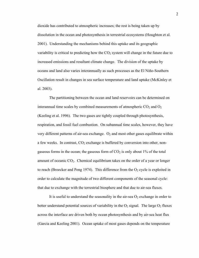
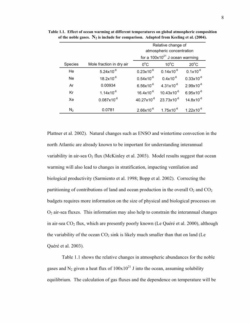
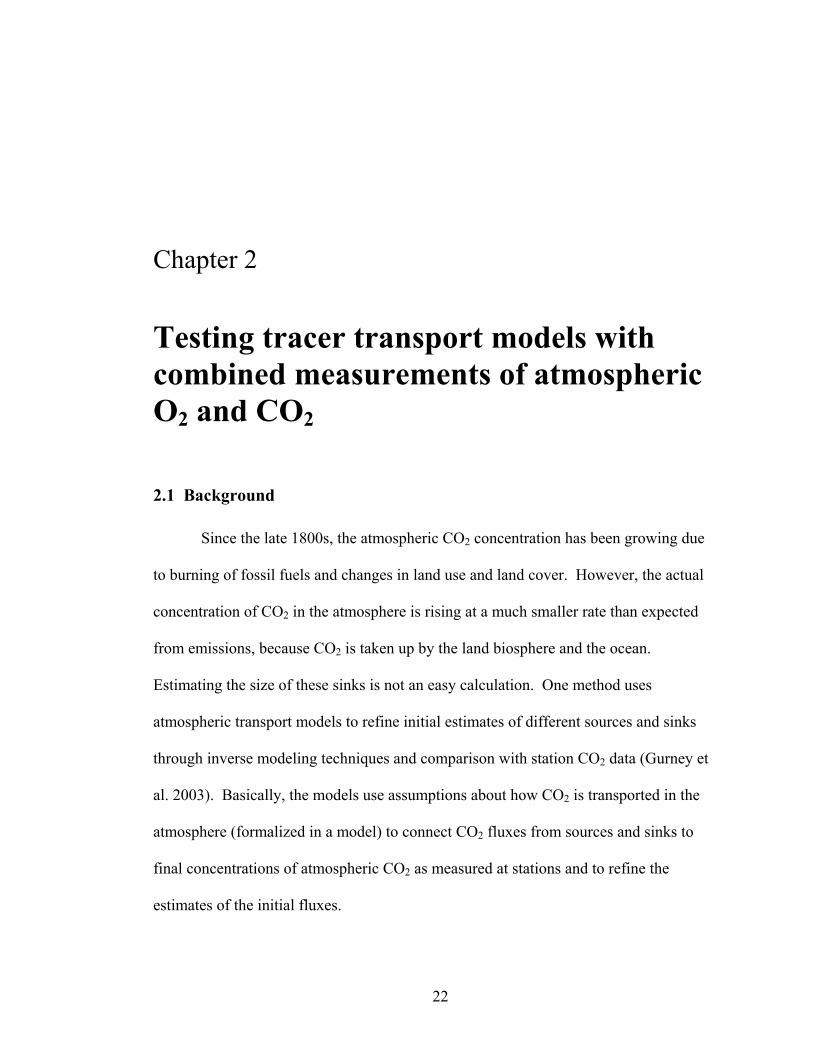
Table 1.1. Effect of ocean warming at different temperatures on global atmospheric composition of the noble gases. N2 is include for comparison. Adapted from Keeling et al. (2004).
Relative change ofatmospheric concentration
for a 100x1021 J ocean warmingSpecies Mole fraction in dry air 0oC 10oC 20oC
He 5.24x10⁻⁶ 0.23x10⁻⁶ 0.14x10⁻⁶ 0.1x10⁻⁶
Ne 18.2x10⁻⁶ 0.54x10⁻⁶ 0.4x10⁻⁶ 0.33x10⁻⁶
Ar 0.00934 6.56x10⁻⁶ 4.31x10⁻⁶ 2.99x10⁻⁶
Kr 1.14x10⁻⁶ 16.4x10⁻⁶ 10.43x10⁻⁶ 6.95x10⁻⁶
Xe 0.087x10⁻⁶ 40.27x10⁻⁶ 23.73x10⁻⁶ 14.8x10⁻⁶
N2 0.0781 2.66x10⁻⁶ 1.75x10⁻⁶ 1.22x10⁻⁶
Plattner et al. 2002). Natural changes such as ENSO and wintertime convection in the
north Atlantic are already known to be important for understanding interannual
variability in air-sea O2 flux (McKinley et al. 2003). Model results suggest that ocean
warming will also lead to changes in stratification, impacting ventilation and
biological productivity (Sarmiento et al. 1998; Bopp et al. 2002). Correcting the
partitioning of contributions of land and ocean production in the overall O2 and CO2
budgets requires more information on the size of physical and biological processes on
O2 air-sea fluxes. This information may also help to constrain the interannual changes
in air-sea CO2 flux, which are presently poorly known (Le Quéré et al. 2000), although
the variability of the ocean CO2 sink is likely much smaller than that on land (Le
Quéré et al. 2003).
Table 1.1 shows the relative changes in atmospheric abundances for the noble
gases and N2 given a heat flux of 100x1021 J into the ocean, assuming solubility
equilibrium. The calculation of gas fluxes and the dependence on temperature will be
9
discussed more thoroughly in Chapter 3. For now, it is useful to note that the ratios
using heavier noble gases, such as Kr/N2 or Xe/N2, should be more sensitive to air-sea
heat flux. However, because their atmospheric concentrations are so small, it would
be necessary to concentrate samples before analysis.
This dissertation primarily concentrates on establishing a long-term
measurement program of atmospheric Ar/N2, balancing the size of the expected
change due to air-sea heat flux with the complexity of the measurement technique.
Although many of the scientific issues discussed above are beyond the scope of this
work, they give an idea of the range of questions that an atmospheric tracer of air-sea
heat flux could help address and their scientific significance. This work instead
focuses on the development of a new measurement technique and what can be learned
from seasonal patterns of tracers of air-sea heat exchange and the impact on
atmospheric gas cycles. Such initial steps will lay the groundwork for interpretation
of a long-term record.
1.2 Atmospheric geochemistry
Dry air is primarily made up of three elements: nitrogen (~78%), oxygen
(~21%), and argon (~1%) with many other trace gases, of which CO2 is the most
common (~0.03%). Although the mean concentrations of the major gases were
determined more than 50 years ago (summarized in Glueckauf (1951)), and the
seasonal cycle in CO2 concentration and other trace gases has been monitored for
several decades, the seasonal cycle in O2 concentration has only been measured for the
10
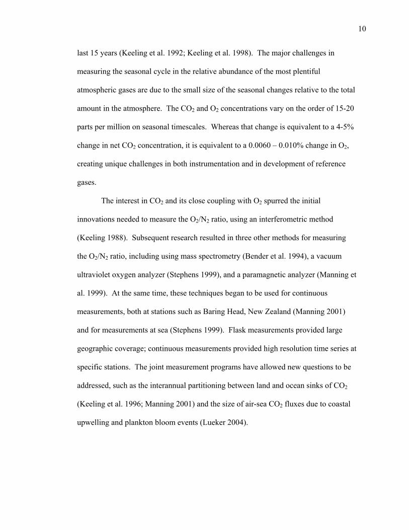
last 15 years (Keeling et al. 1992; Keeling et al. 1998). The major challenges in
measuring the seasonal cycle in the relative abundance of the most plentiful
atmospheric gases are due to the small size of the seasonal changes relative to the total
amount in the atmosphere. The CO2 and O2 concentrations vary on the order of 15-20
parts per million on seasonal timescales. Whereas that change is equivalent to a 4-5%
change in net CO2 concentration, it is equivalent to a 0.0060 – 0.010% change in O2,
creating unique challenges in both instrumentation and in development of reference
gases.
The interest in CO2 and its close coupling with O2 spurred the initial
innovations needed to measure the O2/N2 ratio, using an interferometric method
(Keeling 1988). Subsequent research resulted in three other methods for measuring
the O2/N2 ratio, including using mass spectrometry (Bender et al. 1994), a vacuum
ultraviolet oxygen analyzer (Stephens 1999), and a paramagnetic analyzer (Manning et
al. 1999). At the same time, these techniques began to be used for continuous
measurements, both at stations such as Baring Head, New Zealand (Manning 2001)
and for measurements at sea (Stephens 1999). Flask measurements provided large
geographic coverage; continuous measurements provided high resolution time series at
specific stations. The joint measurement programs have allowed new questions to be
addressed, such as the interannual partitioning between land and ocean sinks of CO2
(Keeling et al. 1996; Manning 2001) and the size of air-sea CO2 fluxes due to coastal
upwelling and plankton bloom events (Lueker 2004).
11
At this point, the atmospheric cycles in O2 and CO2 are comparatively well-
understood. In contrast, almost nothing is known about atmospheric cycles in Ar
abundance, although it is the third most abundant component of the atmosphere.
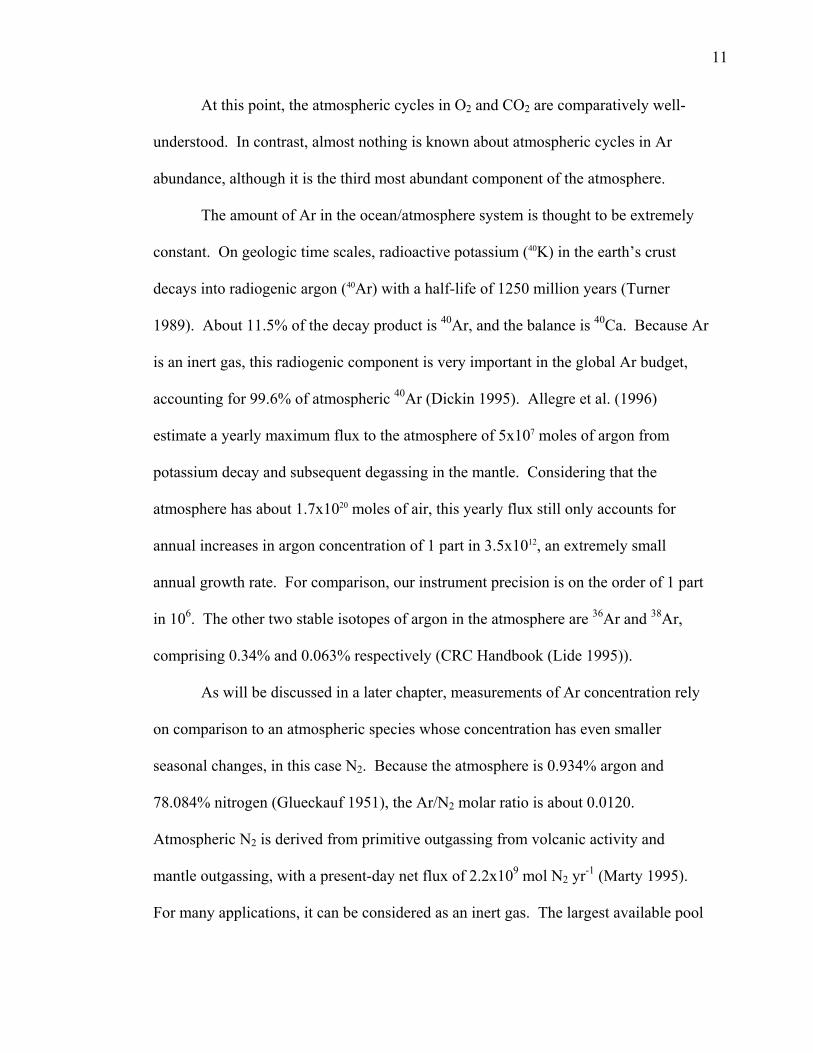
The amount of Ar in the ocean/atmosphere system is thought to be extremely
constant. On geologic time scales, radioactive potassium (40K) in the earth’s crust
decays into radiogenic argon (40Ar) with a half-life of 1250 million years (Turner
1989). About 11.5% of the decay product is 40Ar, and the balance is 40Ca. Because Ar
is an inert gas, this radiogenic component is very important in the global Ar budget,
accounting for 99.6% of atmospheric 40Ar (Dickin 1995). Allegre et al. (1996)
estimate a yearly maximum flux to the atmosphere of 5x10⁷ moles of argon from
potassium decay and subsequent degassing in the mantle. Considering that the
atmosphere has about 1.7x10²⁰ moles of air, this yearly flux still only accounts for
annual increases in argon concentration of 1 part in 3.5x10¹², an extremely small
annual growth rate. For comparison, our instrument precision is on the order of 1 part
in 106. The other two stable isotopes of argon in the atmosphere are 36Ar and 38Ar,
comprising 0.34% and 0.063% respectively (CRC Handbook (Lide 1995)).
As will be discussed in a later chapter, measurements of Ar concentration rely
on comparison to an atmospheric species whose concentration has even smaller
seasonal changes, in this case N2. Because the atmosphere is 0.934% argon and
78.084% nitrogen (Glueckauf 1951), the Ar/N2 molar ratio is about 0.0120.
Atmospheric N2 is derived from primitive outgassing from volcanic activity and
mantle outgassing, with a present-day net flux of 2.2x10⁹ mol N2 yr-1 (Marty 1995).
For many applications, it can be considered as an inert gas. The largest available pool
12
of N2 is located in the atmosphere, with 3.9x10²¹ g. In comparison, only ~100-
145x1015 g is contained in soils and land biota (Schlesinger 1997), with another
570x1015 g contained in the oceans (Pilson 1998). With a flux of about 460x1012 g N
yr-1 due to biological fixation and denitrification both on land and in the ocean
(Schlesinger 1997), the net effect on the atmospheric N2 concentration due to a
seasonal biological cycle is negligible. However, the assumption that biological
activity does not influence the seasonal cycle of atmospheric N2 may be inaccurate in
coastal areas, where biological pulses can release 0.2 x10¹² ± >70% g N2O-N yr-1
(Nevison et al. 2004) and potentially much larger pulses of N2. On short time scales,
these pulses could change the local atmospheric concentration of N2.
Even if not for the critical role that Ar/N2 measurements could play in
understanding questions of heat, research into its atmospheric cycle would be of
interest to the field of geochemistry.
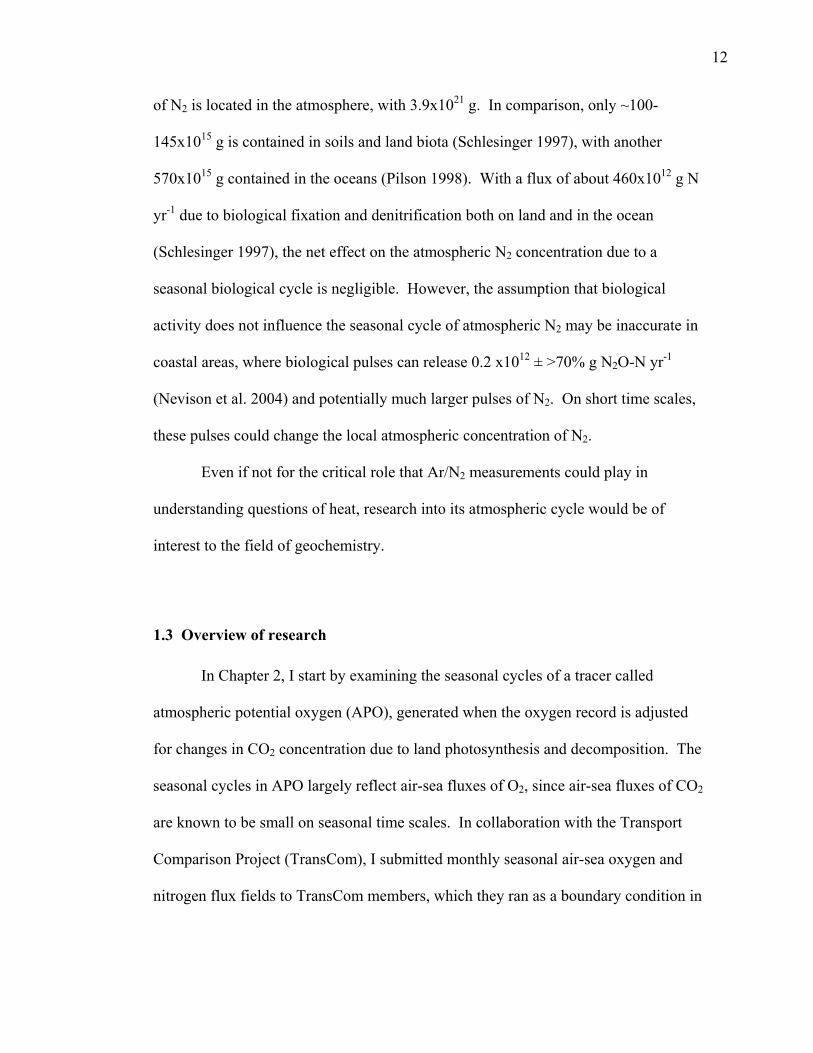
1.3 Overview of research
In Chapter 2, I start by examining the seasonal cycles of a tracer called
atmospheric potential oxygen (APO), generated when the oxygen record is adjusted
for changes in CO2 concentration due to land photosynthesis and decomposition. The
seasonal cycles in APO largely reflect air-sea fluxes of O2, since air-sea fluxes of CO2
are known to be small on seasonal time scales. In collaboration with the Transport
Comparison Project (TransCom), I submitted monthly seasonal air-sea oxygen and
nitrogen flux fields to TransCom members, which they ran as a boundary condition in
13
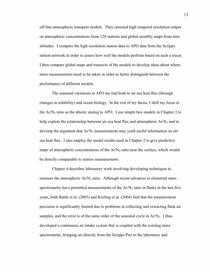
off-line atmospheric transport models. They returned high temporal resolution output
on atmospheric concentrations from 120 stations and global monthly maps from nine
altitudes. I compare the high resolution station data to APO data from the Scripps
station network in order to assess how well the models perform based on such a tracer.
I then compare global maps and transects of the models to develop ideas about where
more measurements need to be taken in order to better distinguish between the
performance of different models.
The seasonal variations in APO are tied both to air-sea heat flux (through
changes in solubility) and ocean biology. In the rest of my thesis, I shift my focus to
the Ar/N2 ratio as the abiotic analog to APO. I use simple box models in Chapter 3 to
help explain the relationship between air-sea heat flux and atmospheric Ar/N2 and to
develop the argument that Ar/N2 measurements may yield useful information on air-
sea heat flux. I also employ the model results used in Chapter 2 to give predictive
maps of atmospheric concentrations of the Ar/N2 ratio near the surface, which would
be directly comparable to station measurements.
Chapter 4 describes laboratory work involving developing techniques to
measure the atmospheric Ar/N2 ratio. Although recent advances in elemental mass
spectrometry have permitted measurements of the Ar/N2 ratio in flasks in the last five
years, both Battle et al. (2003) and Keeling et al. (2004) find that the measurement
precision is significantly limited due to problems in collecting and extracting flask air
samples, and the error is of the same order of the seasonal cycle in Ar/N2. I thus
developed a continuous air intake system that is coupled with the existing mass
spectrometer, bringing air directly from the Scripps Pier to the laboratory and
14
bypassing some of the problems inherent in flask measurements. I describe this new
system, as well as some of the technical issues associated with calibration. I also show
that the 17 months of data successfully measures a seasonal cycle of ~9 per meg in
atmospheric Ar/N2 in La Jolla during the period from February 2004 to June 2005.
Chapter 5 provides an in-depth look at the first 17 months of semi-continuous
data. The measured seasonal cycle is compared to regional air-sea heat flux estimates
from the National Center for Environmental Prediction (NCEP) reanalysis output for
the same time period and found to be within expectations. Parallel measurements of
O2/N2, CO2, and Ar/N2 allow the seasonal cycle in O2/N2 to be partitioned into
components due to land photosynthesis and respiration, air-sea heat flux, and changes
in ocean biology and stratification.
The annual cycle is overlaid with significant synoptic variability on time scales
from one week to a month and which has been observed at this level for the first time.
The correlation between the synoptic variations in Ar/N2 and APO suggest that these
changes may be due to changes in air-sea heat flux or atmospheric transport.
However, the anomalies are not clearly driven by regional or local changes in air-sea
heat flux. It is possible that instrumental issues remain to be worked out, but the
anomalies may also hint at unexpected complexities in the atmospheric Ar/N2 cycle.
These results have significant implications for improving flask measurements
of Ar/N2. One of the important developments in this thesis is the recognition of
thermal fractionation of up to 60 per meg at a sampling inlet (Chapter 4), which may
be one of the reasons that flask measurements show so much variability. Commercial
aspirators have already begun to be installed at the Scripps network of flask stations.
15
Also, if the synoptic variability in the Ar/N2 concentration turns out to be real rather
than an artifact of instrumental problems, such knowledge may be critical to analyzing
and interpreting station flask measurements.
It is planned that the semi-continuous measurement system will continue to be
maintained and improved at the La Jolla station. As the record of atmospheric Ar/N2
grows longer, it will provide useful information on interannual changes in the size and
timing of air-sea heat flux and ocean heat storage and new knowledge about the
atmospheric geochemistry of argon.
16
1.4 Bibliography
Allegre, C. J., A. Hofmann, and K. O’Nions. 1996. The argon constraints on mantle structure. Geophys. Res. Lett. 23: 3555-3557.
Antonov, J. I., S. Levitus, and T. P. Boyer. 2004. Climatological annual cycle of
ocean heat content. Geophys. Res. Lett. 31: (doi: 10.1029/2003GL018851). Barnett, T. P., D. W. Pierce, K. M. AchutaRao, P. J. Gleckler, B. D. Santer, J. M.
Gregory, and W. M. Washington. 2005. Penetration of human-induced warming into the world’s oceans. Science 309: 284-287.
Battle, M., M. Bender, M. B. Hendricks, D. T. Ho, R. Mika, G. McKinley, S.-M. Fan,
T. Blaine, and R. F. Keeling. 2003. Measurements and models of the atmospheric Ar/N2 ratio. Geophys. Res. Lett. 30 (doi: 10.1029/2003GL017411).
Bender, M. L., P. P. Tans, J. T. Ellis, J. Orchardo, and K. Habfast. 1994. A high
precision isotope ratio mass spectrometry method for measuring the O2/N2 ratio of air. Geochim. Cosmochim. Acta 58: 4751-4758.
Bopp, L., C. Le Quéré, M. Heimann, and A. C. Manning. 2002. Climate-induced
oceanic oxygen fluxes: Implications for the contemporary carbon budget. Glob. Biogeochem. Cycles 16 (doi: 10.1029/2001GB001445).
Bowman, K. P. and J. P. Cohen. 1997. Interhemispheric exchange by seasonal
modulation of the Hadley circulation. J. Atmos. Sci. 54: 2045-2059. Broecker, W. S. and T.-H. Peng. 1974. Gas exchange rates between air and sea.
Tellus 26: 21-35. Cohen-Solal, E. And H. Le Treut. 1997. Role of the oceanic heat transport in climate
dynamics: A sensitivity study with an atmospheric general circulation model. Tellus 49A: 371-387.
Conkright, M. E., J.I. Antonov, O. Baranova, T. P. Boyer, H.E. Garcia, R. Gelfeld, D.
Johnson, R.A. Locarnini, P.P. Murphy, T.D. O'Brien, I. Smolyar, C. Stephens, 2002: World Ocean Database 2001, Volume 1: Introduction. Ed: Sydney Levitus, NOAA Atlas NESDIS 42. U.S. Government Printing Office: Washington, D.C.
Lide, D. R., ed. 1995. CRC Handbook of Chemistry and Physics (76th edition). CRC
Press, Inc.: Boca Raton, FL.
17
Dickin, A. P. 1995 (1997 paperback edition). Radiogenic Isotope Geology. Cambridge University Press: Cambridge, U.K.
Ganachaud, A. and C. Wunsch. 2000. Improved estimates of global ocean
circulation, heat transport and mixing from hydrographic data. Nature 408: 453-457.
Ganachaud, A. and C. Wunsch. 2003. Large-scale ocean heat and freshwater
transports during the World Ocean Circulation Experiment. J. Clim. 16: 696-705.
Garcia, H. E. and R. F. Keeling. 2001. On the global oxygen anomaly and air-sea
flux. J. Geophys. Res. 106: 31,155-31,166. Geller, L. S., J. W. Elkins, J. M. Lobert, A. D. Clarke, D. F. Hurst, J. H. Butler, and R.
C. Myers. 1997. Tropospheric SF6: Observed latitudinal distributioni and trends, derived emissions and Interhemispheric exchange time. Geophys. Res. Lett. 24: 675-678.
Gloor, M., N. Gruber, T. M. C. Hughes, and J. L. Sarmiento. 2001. Estimating net
air-sea fluxes from ocean bulk data: Methodology and application to the heat cycle. Glob. Biogeochem. Cycles 15: 767-782.
Glueckauf, E. 1951. The composition of atmospheric air. Compendium of
Meteorology. Am. Met. Soc. Boston, 3-11. Graber, H. C., E. A. Terray, M. A. Donelan, W. M. Drennan, J. C. Van Leer, and D.
B. Peters. 2000. ASIS – A new air-sea interaction spar buoy: design and performance at sea. J. Atmos. Ocean. Tech. 17: 708-720.
Gregory, J. M., H. T. Banks, P. A. Stott, J. A. Lowe, and M. D. Palmer. 2004.
Simulated and observed decadal variability in ocean heat content. Geophys. Res. Lett. 31 (doi: 10.1029/2004GL020258).
Hansen, J., L. Nazarenko, R. Ruedy, M. Sato, J. Willis, A. Del Genio, D. Koch, A.
Lacis, K. Lo, S. Menon, T. Novakov, J. Perlwitz, G. Russell, G. A. Schmidt, and N. Tausnev. 2005. Earth’s energy imbalance: confirmation and implications. Science 308: 1431-1435.
Hasse, L. and S. D. Smith. 1997. Local sea surface wind, wind stress, and sensible
and latent heat fluxes. J. Clim. 10: 2711-2724. Hazeleger, W., R. Seager, M. A. Cane, and N. H. Naik. 2004. How can tropical
Pacific Ocean heat transport vary? J. Phys. Oceanogr. 34: 320-333.
18
Held, I. M. 2001. The partitioning of the poleward energy transport between the tropical ocean and atmosphere. J. Atmos. Sci. 58: 943-948.
Houghton, J. T., Y. Ding, D. J. Griggs, M. Noguer, P. J. van der Linden, X. Dai, K.
Maskell, and C. A. Johnson (eds). 2001. Climate Change 2001: The Scientific Basis (Contribution of Working Group I to the Third Assessment Report of the Intergovernmental Panel on Climate Change). Cambridge University Press: Cambridge, U.K., and New York, U.S.A.
Jayne, S. R. and J. Marotzke. 2001. The dynamics of ocean heat transport variability.
Rev. Geophys. 39: 385-411. Jo, Y.-H., X.-H. Yan, J. Pan, W. T. Liu, and M.-X. He. 2004. Sensible and latent heat
flux in the tropical Pacifi from satellite multi-sensor data. Remote Sens. Environ. 90: 166-177.
Josey, S. A., E. C. Kent, and P. K. Taylor. 1999. New insights into the ocean heat
budget closure problem from analysis of the SOC air-sea flux climatology. J. Clim. 12: 2856-2880.
Keeling, R. F. 1988. Development of an interferometric oxygen analyzer for precise
measurement of the atmospheric O2 mole fraction. Ph.D. thesis: Harvard University, Cambridge, Massachusetts.
Keeling, R. F., T. Blaine, B. Paplawsky, L. Katz, C. Atwood, and T. Brockwell. 2004.
Measurement of changes in atmospheric Ar/N2 ratio using a rapid-switching, single-capillary mass spectrometer system. Tellus 56B: 322-388.
Keeling, R. F., and H. E. Garcia. 2002. The change in oceanic O2 inventory
associated with recent global warming. Proc. Natl. Acad. Sci. USA 99 (doi: 10.1073/pnas.122154899).
Keeling, R. F., A. C. Manning, E. M. McEvoy, and S. R. Shertz. 1998. Methods for
measuring changes in atmospheric O2 concentration and their application in southern hemisphere air. J. Geophys. Res. 103: 3381-3397.
Keeling, R. F., S. C. Piper, and M. Heimann. 1996. Global and hemispheric CO2
sinks deduced from changes in atmospheric O2 concentration. Nature 381: 218-221.
Keeling, R. F. and S. R. Shertz. 1992. Seasonal and interannual variations in
atmospheric oxygen and implications for the global carbon cycle. Nature 358: 723-727.
19
Keith, D. W. 1995. Meridional energy transport: uncertainty in zonal means. Tellus 47A: 30-44.
Kelly, K. A. 2004. The relationship between oceanic heat transport and surface
fluxes in the western North Pacific: 1970-2000. J. Clim. 17: 573-588. Le Quéré, C., O. Aumont, L. Bopp, P. Bousquet, P. Ciais, R. Francey, M. Heimann, C.
D. Keeling, R. F. Keeling, H. Kheshgi, P. Peylin, S. C. Piper, I. C. Prentice, and P. J. Rayner. 2003. Two decades of ocean CO2 sink and variability. Tellus 55B: 649-656.
Le Quéré, C., J. C. Orr, P. Monfray, O. Aumont, and G. Madec. 2000. Interannual
variability of the oceanic sink of CO2 from 1979 through 1997. Glob. Biogeochem. Cycles 14: 1247-1265.
Levitus, S., J. Antonov, and T. Boyer. 2005. Warming of the world ocean, 1955-
2003. Geophys. Res. Lett. 32, L02604 (doi: 10.1029/2004GL021592). Levitus, S., J. I. Antonov, T. P. Boyer, and C. Stephens. 2000. Warming of the world
ocean. Science 287: 2225-2228. Levitus, S., J. I. Antonov, J. Wang, T. L. Delworth, K. W. Dixon, and A. J. Broccoli.
2001. Anthropogenic warming of the earth’s climate system. Science 292: 267-270.
Liss, P. S. and L. Merlivat. 1986. Air-sea gas exchange rates: introduction and
synthesis. Pages 113-127 in: P. Buat-Ménard (ed.). The Role of Air-Sea Exchange in Geochemical Cycling. D. Reidel Publishing Co.: Norwell, Mass.
Lueker, T. J. 2004. Coastal upwelling fluxes of O2, N2O, and CO2 assessed from
continuous atmospheric observations at Trinidad, California. Biogeosciences 1: 101-111.
Manning, A. C. 2001. Temporal variability of atmospheric oxygen from both
continuous measurements and a flask sampling network: Tools for studying the global carbon cycle. Ph.D. thesis: University of California, San Diego, La Jolla, CA.
Manning, A.C., R. F. Keeling, and J. P. Severinghaus. 1999. Precise atmospheric
oxygen measurements with a paramagnetic oxygen analyzer. Glob. Biogeochem. Cycles 113: 1107-115.
Marty, B. 1995. Nitrogen content of the mantle inferred from N2-Ar correlation in
oceanic basalts. Nature 377: 326-329.
20
McKinley, G. A., M. J. Follows, and J. Marshall. 2003. Interannual variability of air-sea O2 fluxes and the determination of CO2 sinks using atmospheric O2/N2. Geophys. Res. Lett. 30 (doi: 10.1029/2002GL016044).
Nevison, C. D., T. J. Lueker, and R. F. Weiss. 2004. Quantifying the nitrous oxide
source from coastal upwelling. Glob. Biogeochem. Cycles 18, GB1018 (doi: 10.1029/2003GB002110).
Nightingale, P. D., G. Malin, C. S. Law, A. J. Watson, P. S. Liss, M. I. Liddicoat, J.
Boutin, and R. C. Upstill-Goddard. 2000. In situ evaluation of air-sea gas exchange parameterizations using novel conservative and volatile tracers. Glob. Biogeochem. Cycles 14: 373-387.
Peixoto, J. P. and A. H. Oort. 1992. Physics of Climate. American Institute of
Physics: New York. Pielke, R. A., Sr. 2003. Heat storage within the earth system. Bull. Am. Meteorol.
Soc. 84: 331-335. Pilson, M. E. Q. 1998. An Introduction to the Chemistry of the Sea. Prentice-Hall,
Inc.: New Jersey. Plattner, G.-K., F. Joos, and T. F. Stocker. 2002. Revision of the global carbon
budget due to changing air-sea oxygen fluxes. Glob. Biogeochem. Cycles 16 (doi: 10.1029/2001GB001746).
Reichert, B. K., R. Schnur, and L. Bengtsson. 2002. Global ocean warming tied to
anthropogenic forcing. Geophys. Res. Lett. 29 (doi: 10.1029/2001GL013954). Sarmiento, J. L., T. M. C. Hughes, R. J. Stouffer, and S. Manabe. 1998. Simulated
response of the ocean carbon cycle to anthropogenic climate warming. Nature 393: 245-249.
Schlesinger, W. H. 1997. Biogeochemisty: An Analysis of Global Change, 2nd ed.
Academic Press: San Diego, CA. Stephens, B. B. 1999. Field-based atmospheric oxygen measurements and the ocean
carbon cycle. Ph.D. thesis: University of California, San Diego, La Jolla, CA. Talley, L. D. 2003. Shallow, intermediate, and deep overturning components of the
global heat budget. J. Phys. Oceanogr. 33: 530-560. Timmerman, A., J. Oberhuber, A. Bacher, M. Esch, M. Latif, and E. Roeckner. 1999.
Increased El Niño frequency in a climate model forced by future greenhouse warming. Nature 398: 694-697.
21
Trenberth, K. E. and J. M. Caron. 2001. Estimates of meridional atmosphere and
ocean heat flux. J. Clim. 14: 3433-3443. Trenberth, K. E., J. M. Caron, and D. P. Stepaniak. 2001. The atmospheric energy
budget and implications for surface fluxes and ocean heat transports. Clim. Dyn. 17: 259-276.
Turner, G. 1989. The outgassing history of the Earth’s atmosphere. J. Geolog. Soc.
London 146: 147-154. Wanninkhof, R. 1992. Relationship between wind speed and gas exchange over the
ocean. J. Geophys. Res. 97: 7373-7382. Willis, J. K., D. Roemmich, and B. Cornuelle. 2003. Combining altimetric height
with broadscale profile data to estimate steric height, heat storage, subsurface temperature, and sea-surface temperature variability. J. Geophys. Res. 108 (doi: 10.1029/2002JC001755).
Willis, J. K., D. Roemmich, and B. Cornuelle. 2004. Interannual variability in upper
ocean heat content, temperature, and thermosteric expansion on global scales. J. Geophys. Res. 109 (doi: 10.1029/2003JC002260).
22
Chapter 2
Testing tracer transport models with combined measurements of atmospheric O2 and CO2
2.1 Background
Since the late 1800s, the atmospheric CO2 concentration has been growing due
to burning of fossil fuels and changes in land use and land cover. However, the actual
concentration of CO2 in the atmosphere is rising at a much smaller rate than expected
from emissions, because CO2 is taken up by the land biosphere and the ocean.
Estimating the size of these sinks is not an easy calculation. One method uses
atmospheric transport models to refine initial estimates of different sources and sinks
through inverse modeling techniques and comparison with station CO2 data (Gurney et
al. 2003). Basically, the models use assumptions about how CO2 is transported in the
atmosphere (formalized in a model) to connect CO2 fluxes from sources and sinks to
final concentrations of atmospheric CO2 as measured at stations and to refine the
estimates of the initial fluxes.
23
The Atmospheric Tracer Transport Model Intercomparison Project TransCom)
has its roots in the 4th International CO2 conference in 1993. A collaboration between
modeling groups, it was created to assess and analyze the behavior and transport
algorithms of atmospheric tracer transport models (Denning et al. 1999). For a
particular project, each participating research group uses the same shared datasets of
gas fluxes from sources and sinks as input into their tracer transport model. The
model predictions of atmospheric concentrations are then submitted in a standardized
format to a central computer server, where any member of the group can access the
output. The first two studies centered on forward simulations to compare model
predictions with atmospheric measurements: Law et al. (1996) used estimates of CO2
emissions from both fossil fuel and land biology; Denning et al. (1999) employed
sulfur hexafluoride (SF6), which has similar spatial patterns of anthropogenic
emissions to CO2 but no biological source. The third project concentrated on inverse
calculations of carbon dioxide sources and sinks on annual mean, seasonal, and
interannual time scales, as well as evaluating the sensitivity of the results to the choice
of data used (Gurney et al. 2002, Gurney et al. 2003, Law et al. 2003, Gurney et al.
2004).
One of the weaknesses associated with transport models has to do with a lack
of understanding of the “rectifier effect” – the relationship between seasonal changes
in fluxes and transport. In general, both tracer concentrations and the time scale of
atmospheric transport can be broken into seasonal and annual mean components for
analysis. However, the interaction of seasonal fluxes and seasonal changes in
24
atmospheric transport can lead to a mean annual signal, known as the rectifier.
Likewise, the mean annual fluxes and transport can lead to a seasonal signal (Keeling
et al. 1993). Models may not be accurately reflecting seasonal changes in transport
and fluxes, which may lead to problems in both forward predictions and inverse
analyses.
This study extends the earlier TransCom work by building an understanding of
atmospheric transport of an oceanic tracer on seasonal time scales. The tracer chosen
for this analysis is atmospheric potential oxygen (APO), as defined by Stephens et al.
(1998). APO is effectively the amount of O2 that would be present in an air parcel if
land photosynthesis drew CO2 down to zero. Based on the stoichiometric relationship
between O2 and CO2 in terrestrial photosynthesis and respiration (Keeling 1988;
Severinghaus 1995), APO is conservative to land biology but reflects the oceanic
component in the atmospheric CO2 and O2/N2 cycles. On seasonal time scales (the
focus of this study), the oceanic O2 exchange is much larger than the CO2 exchange,
because the equilibration time for oceanic CO2 is 12-20 times longer than for most
other gases. As carbon is stored primarily in carbonate and bicarbonate, the reactions
between dissolved CO2 and these species buffer the air-sea CO2 flux (Keeling et al.
1993). Like the air-sea CO2 exchange, the combustion of fossil fuels contributes very
little in seasonality in APO in comparison to the size of air-sea fluxes of oxygen. The
seasonal cycle in APO thus is effectively equivalent to the oceanic component of the
O2/N2 cycle.
25
The seasonal air-sea oxygen flux contribution to the atmospheric O2/N2 cycle
reflects both biological and physical processes across the air-sea interface. Biological
processes include marine production and remineralization of organic matter. Physical
processes include air-sea gas exchange, water ventilation, solubility changes driven by
temperature changes, and near-surface turbulence and mixing (Garcia and Keeling
2001). The seasonal cycle is characterized by a net O2 flux into the atmosphere during
spring and summer, whereas the fall and winter are characterized by a net flux out of
the atmosphere and into the ocean (Najjar and Keeling 2000). There is also a small
thermal component in N2, which reduces the amplitude of the overall O2/N2 ratio by
about 10%. These seasonally varying fluxes are small in equatorial areas and largest
between 30-60o in each hemisphere where the seasonal air-sea heat fluxes are largest
(Garcia and Keeling 2001). On top of this seasonal flux is a mean zonal component,
with tropical areas serving as a source of O2 and high-latitude areas serving as a sink
(Stephens et al. 1998).
Recent work has concentrated on developing global maps of seasonal air-sea
O2 fluxes based on the dissolved O2 anomaly in the upper ocean and using these maps
to calculate the air-sea gas exchange velocity. Najjar and Keeling (2000) first
developed such maps, although they are known to have seasonal sparseness of data
that leads to a summertime bias and a possible underestimate of seasonal variations
and overestimate of the annual mean. These fluxes were used as a boundary condition
into the atmospheric transport model TM2 to estimate the air-sea O2 exchange velocity
based on comparison of APO measured at stations (Keeling et al. 1998). The authors
26
concluded that the Wanninkhof (1992) formulation for air-sea gas exchange velocity
performed better than alternative formulations. They further refined the air-sea O2
exchange velocity by calculating regional scaling constants of 1.15±0.05 and
1.23±0.05 in the northern and southern hemispheres, respectively, poleward of 31o.
Although any estimate of low latitudes is likely to have more error, they suggested a
range of values between 0.07 and 0.53 for individual stations.
These results were revised by Garcia and Keeling (2001), who presented a
refined estimate of air-sea O2 fluxes. Using the same transport model, Garcia and
Keeling concluded the Wanninkhof (1992) formulation for air-sea gas transfer
velocities worked well with no scaling coefficient. The results of both of these papers
depend on the accuracy of the atmospheric transport model used. This point will be
relevant later in the discussion of this present work.
APO has previously been used to evaluate models of ocean transport.
Stephens et al. (1998) employed ocean models to predict annual mean air-sea fluxes
and then used the modeled fluxes as input to an atmospheric transport model in order
to compare its predictions with the distribution of atmospheric APO observations. The
study concluded that the oceanic models were underestimating the interhemispheric
gradient in APO and the southward oceanic fluxes of oxygen and carbon dioxide.
High atmospheric APO concentrations were predicted near the equator, where
outgassing led to large air-sea O2 fluxes in the ocean models. However, their
conclusions were limited by lack of any monitoring stations in equatorial areas and by
the ability of the atmospheric transport model to correctly represent transport. A
27
following study using a different atmospheric transport model (Gruber et al. 2001)
suggested that the underestimates of oceanic flux found by Stephens et al. (1998)
could be inaccurate due to problems in the atmospheric transport model used rather
than to problems with the ocean models. More recent measurements of APO in
equatorial areas, however, confirm the “equatorial bulge” and suggest that it is larger
than expected from either of the two previous studies (Battle et al. 2005). These three
papers highlight the importance of better understanding the limitations – and
predictive abilities – of atmospheric transport models.
In the present study, TransCom participants were asked to run seasonal flux
fields of oceanic O2 and N2 in their own atmospheric transport models. Each
modeling group then submitted seasonal model predictions of atmospheric
concentrations to the TransCom program archive, from which I could access the
output. The resulting changes in O2 and N2 in the atmosphere can then be combined to
estimate changes in the O2/N2 ratio, which in turn can be compared to observations.
In this chapter, I compare station-specific model predictions and observations
of seasonal atmospheric APO cycles and the rectifier effect on APO in order to
evaluate the transport models and the flux fields used. I then consider global maps
and transects of APO to further study differences in predictions among the models.
The annual mean component of the air-sea fluxes is not used in this study because the
mean air-sea O2 flux is not well-defined. Any resultant annual mean is thus limited
solely to the interaction between seasonal atmospheric transport patterns and oceanic
variability in sources and sinks. This study thus helps to resolve the size of these
28
cross-terms, or rectifier effects. Lastly, this work may help to pinpoint important areas
where new observations could provide the most sensitive test of models.
2.2 Methods
2.2.1 Surface O2 and N2 fluxes
I submitted global monthly O2 and N2 air-sea flux maps to be used as boundary
conditions for the TransCom model runs. Developed by Garcia and Keeling (2001),
the oxygen flux fields consist of a monthly climatology based on a weighted least
squares fit between historical ocean O2 data and monthly heat flux anomalies. Garcia
and Keeling (2001) use the Wanninkhof (1992) relationship to calculate the air-sea O2
flux from the oceanic O2 anomalies. This approach is based on the empirical finding
that O2 fluxes and heat fluxes are reasonably well correlated. Garcia and Keeling
(2001) exploit the better time resolution in heat flux estimates in order to improve the
space/time resolution in O2 fluxes, improving on the data sparseness problem in the
Najjar and Keeling (2000) oxygen flux fields. This approach assumes that the O2
fluxes are exactly in phase with the heat fluxes. However, the O2 fluxes should have a
lag period associated both with the efficiency of gas equilibration in the mixed layer
with the overlying atmosphere and with the response time of photosynthesis to
seasonal stratification and nutrient availability (Garcia and Keeling 2001). For the
thermal component, a lag of about three week is expected. For the biological
component, it is less clear what to expect, since the biological O2 fluxes and heat
29
fluxes do not have as strong a mechanistic link; however, the lag is likely to be similar
to the thermal lag.
The nitrogen flux fields consist of a global monthly map of N2 ocean fluxes
developed by scaling climatological European Center for Medium-Range Weather
Forecast (ECMWF) heat fluxes from Gibson et al. (1997). The annual mean N2 flux at
every grid point was subtracted from the monthly heat flux fields in order to leave
only the seasonal cycle. Using a monthly sea surface temperature data set (Shea et al.
1992) masked for land and ice and assuming constant salinity, I calculated the
derivative of the Weiss (1970) solubility relationship with respect to temperature at a
given grid point and time. This value was then used with the ECMWF heat fluxes to
compute gas fluxes following Keeling et al. (1993):
Gas Flux = ,⎟⎟⎠
⎞⎜⎜⎝
⎛⎟⎠⎞
⎜⎝⎛−
pcQ
dTdN (2.1)
where (dN/dT) is the change in solubility with temperature for a particular gas (in this
case, N2) in μmol kg-1 oC-1, Q is the heat flux in J m-2 month-1, and cp is the heat
capacity with units of J kg-1 oC-1. This formulation assumes that air-sea heat flux is the
only determinant of the ocean surface concentration of N2 and that surface waters
equilibrate rapidly and completely. Although the N2 cycle does have small biological
influences, they are negligible in this context. The N2 flux fields assume that the
saturation anomalies and thus tracer fluxes depend directly on air-sea heat flux and
equilibrate instantly, although it takes about three weeks for the mixed layer to
equilibrate (Keeling et al. 1993).
30
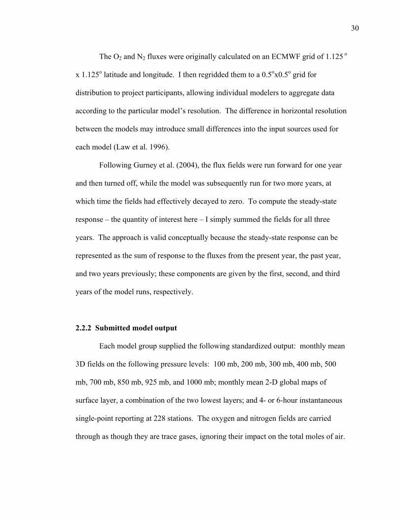
The O2 and N2 fluxes were originally calculated on an ECMWF grid of 1.125 o
x 1.125o latitude and longitude. I then regridded them to a 0.5ox0.5o grid for
distribution to project participants, allowing individual modelers to aggregate data
according to the particular model’s resolution. The difference in horizontal resolution
between the models may introduce small differences into the input sources used for
each model (Law et al. 1996).
Following Gurney et al. (2004), the flux fields were run forward for one year
and then turned off, while the model was subsequently run for two more years, at
which time the fields had effectively decayed to zero. To compute the steady-state
response – the quantity of interest here – I simply summed the fields for all three
years. The approach is valid conceptually because the steady-state response can be
represented as the sum of response to the fluxes from the present year, the past year,
and two years previously; these components are given by the first, second, and third
years of the model runs, respectively.
2.2.2 Submitted model output
Each model group supplied the following standardized output: monthly mean
3D fields on the following pressure levels: 100 mb, 200 mb, 300 mb, 400 mb, 500
mb, 700 mb, 850 mb, 925 mb, and 1000 mb; monthly mean 2-D global maps of
surface layer, a combination of the two lowest layers; and 4- or 6-hour instantaneous
single-point reporting at 228 stations. The oxygen and nitrogen fields are carried
through as though they are trace gases, ignoring their impact on the total moles of air.
31
Thus, the output fields were supplied as mixing ratios in μmole per mole of dry air. I
then combined the two fields to compute changes in the O2/N2 ratio in per meg units
according to:
( ) ,78084.020946.0
2222
NONO −≅δ (2.2)
where “O2” and “N2” designate the equivalent trace gas mixing ratio anomaly
computed by the model in μmole/mole and 0.20946 and 0.78084 reflect the O2 and N2
mole fractions in dry air (Glueckauf 1951).
2.2.3 Model descriptions
The calculations were run with 9 different tracer transport models and model
variants. A tenth (TM2-ECMWF86), which I ran, is included in certain figures early
in this chapter for continuity with previous papers (Garcia and Keeling 2001; Keeling
et al. 1998). The models were submitted by users, rather than developers, although
these roles may overlap in some research groups. Every model used in this chapter is
an off-line version, with winds input from external data sets or atmospheric general
circulation model predictions driving the model rather than using an internal
calculation of the winds. A few of the models have been extensively used and tested
(GCTM, TM2) whereas others have been more recently developed and tested less
extensively (NIES, JMA).
The submitted models can be broken down into related groups. TM2 and TM3
are different versions of a model originally developed by Heimann and Keeling
(1989), which used the monthly vertical convection statistics of the Goddard Institute
32
Space Studies model (GISS) (Heimann 1995). TM2 updates the calculation of
subgrid-scale vertical transport by clouds and turbulent diffusion, and TM3 has a
higher spatial and vertical resolution. NIRE is also related to the GISS model,
although it uses a different advection scheme. Two other models, NIES and JMA-
CDTM, are both offshoots of the NIRE model.
MATCH and GCTM are more independent of the GISS history. MATCH
shares components of the National Center for Atmospheric Research Community
Climate Model (CCM, Rasch et al. 1997), which is not used in this study. GCTM was
first developed at the National Oceanic and Atmospheric Administration Geophysical
Fluid Dynamics Laboratory in the early 1970s (Mahlman and Moxim 1978).
All of these models vary in resolution and in their transport characteristics (see
Table 2.1 for a summary of the model characteristics). Many share similar
parameterizations, but not all have parameterizations for certain characteristics, such
as horizontal diffusion or convection related to cloud formation. Some explicitly
model a planetary boundary layer, others do not. These choices result from various
priorities in each model’s development and lead to some recognized differences in
predictive ability. For example, JMA, first developed in the aftermath of the
Chernobyl accident by the Japan Meteorological Agency, overestimates ground-level
concentrations in the short term (less than 24 hours), probably because of weak
vertical diffusion (Iwasaki et al. 1998). NIES is known to have a faster vertical
transport than NIRE but slower than GISS (Maksyutov and Inoue 2000). GFDL has
weak vertical mixing out of the surface layer, resulting in higher surface peak values
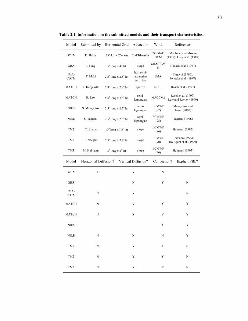
33
Table 2.1 Information on the submitted models and their transport characteristics.
Model Submitted by Horizontal Grid Advection Wind References
GCTM D. Baker 256 km x 256 km 2nd/4th order ZODIAC GCM
Mahlman and Moxim (1978); Levy et al. (1982)
GISS I. Fung 5o long x 4o lat slope GISS CGM II Hansen et al. (1997)
JMA-CDTM T. Maki 2.5o long x 2.5o lat
hor: semi-lagrangian, vert: box
JMA Taguchi (1996); Iwasaki et al. (1998)
MATCH R. Dargaville 2.8o long x 2.8o lat spitfire NCEP Rasch et al. (1997)
MATCH R. Law 5.6o long x 2.8o latsemi-
lagrangian MACCM2 Rasch et al. (1997); Law and Rayner (1999)
NIES S. Maksyutov 2.5o long x 2.5o latsemi-
lagrangianECMWF
(97)Maksyutov and Inoue (2000)
NIRE S. Taguchi 2.5o long x 2.5o latsemi-
lagrangianECMWF
(95) Taguchi (1996)
TM2 T. Blaine 10o long x 7.5o lat slope ECMWF (86) Heimann (1995)
TM2 T. Naegler 7.5o long x 7.2o lat slope ECMWF (90)
Heimann (1995); Bousquet et al. (1999)
TM3 M. Heimann 5o long x 4o lat slope ECMWF (90) Heimann (1995)
Model Horizontal Diffusion? Vertical Diffusion? Convection? Explicit PBL?
GCTM Y Y N
GISS N Y N
JMA-CDTM N Y N
MATCH N Y Y Y
MATCH N Y Y Y
NIES Y Y
NIRE N N N Y
TM2 N Y Y N
TM2 N Y Y N
TM3 N Y Y N
34
in the source distribution better. Likewise, TM2 is known to display a smaller rectifier
effect above continent, probably due to its coarse resolution, whereas TM3 generally
displays a larger rectifier (Bousquet et al. 1999; Law et al. 1996). All of these
characteristics will contribute to the predictive abilities of particular models in dealing
with APO. Previous TransCom results highlight the importance of subgrid-scale
parameterized vertical transport, more than any other parameterization, for explaining
the difference between models and accurately representing atmospheric concentrations
of a tracer (Denning et al. 1999).
2.3 Results
2.3.1 Comparison of station measurements and model predictions
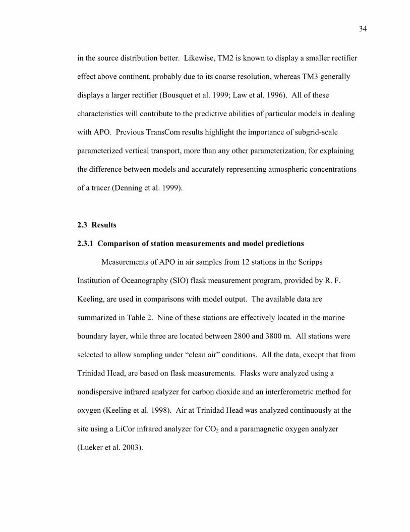
Measurements of APO in air samples from 12 stations in the Scripps
Institution of Oceanography (SIO) flask measurement program, provided by R. F.
Keeling, are used in comparisons with model output. The available data are
summarized in Table 2. Nine of these stations are effectively located in the marine
boundary layer, while three are located between 2800 and 3800 m. All stations were
selected to allow sampling under “clean air” conditions. All the data, except that from
Trinidad Head, are based on flask measurements. Flasks were analyzed using a
nondispersive infrared analyzer for carbon dioxide and an interferometric method for
oxygen (Keeling et al. 1998). Air at Trinidad Head was analyzed continuously at the
site using a LiCor infrared analyzer for CO2 and a paramagnetic oxygen analyzer
(Lueker et al. 2003).
35
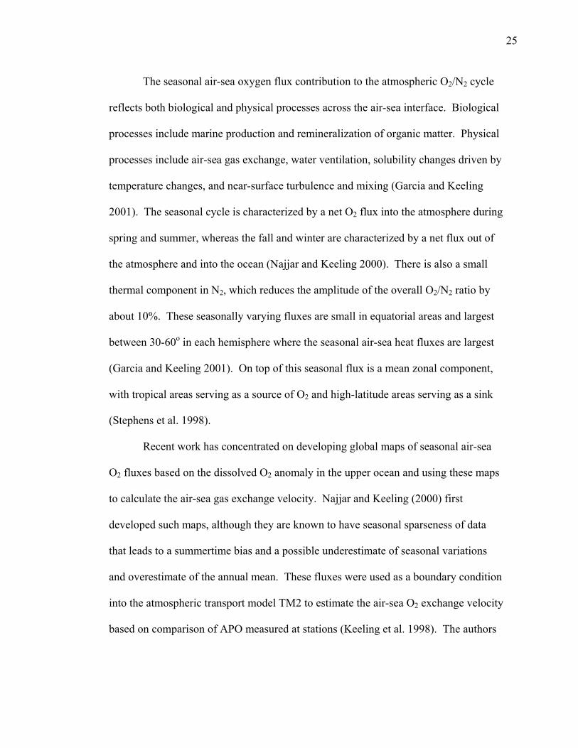
60oE 120oE 180oW 120oW 60oW 0o 90oS
60oS
30oS
0o
30oN
60oN
90oN Alert
Cold Bay
Trinidad HeadLa Jolla
Mauna LoaKumukahi
Samoa
Cape Grim
Palmer Station
South Pole
Niwot Ridge
Macquarie Island
60oE 120oE 180oW 120oW 60oW 0o 90oS
60oS
30oS
0o
30oN
60oN
90oN Alert
Cold Bay
Trinidad HeadLa Jolla
Mauna LoaKumukahi
Samoa
Cape Grim
Palmer Station
South Pole
Niwot Ridge
Macquarie Island
Current sampling stationDiscontinued sampling station
Figure 2.1. Map of the locations of stations with data used for comparison with models.
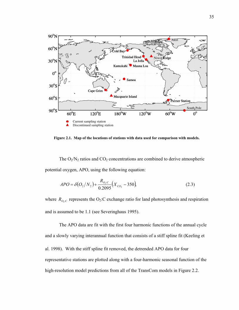
The O2/N2 ratios and CO2 concentrations are combined to derive atmospheric
potential oxygen, APO, using the following equation:
( ) ( ),3502095.0 2
2:22 −+= CO
CO XR
NOAPO δ (2.3)
where COR :2 represents the O2:C exchange ratio for land photosynthesis and respiration
and is assumed to be 1.1 (see Severinghaus 1995).
The APO data are fit with the first four harmonic functions of the annual cycle
and a slowly varying interannual function that consists of a stiff spline fit (Keeling et
al. 1998). With the stiff spline fit removed, the detrended APO data for four
representative stations are plotted along with a four-harmonic seasonal function of the
high-resolution model predictions from all of the TransCom models in Figure 2.2.
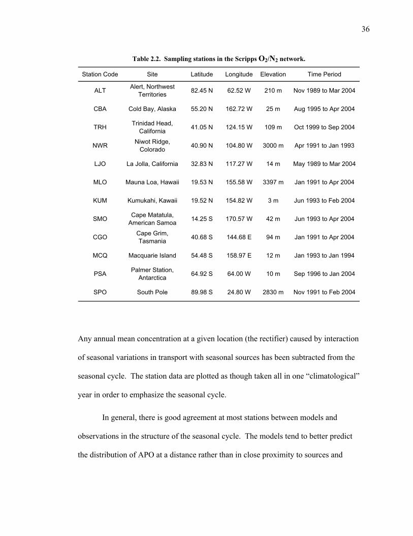
36
Table 2.2. Sampling stations in the Scripps O2/N2 network.
Station Code Site Latitude Longitude Elevation Time Period
ALT Alert, Northwest Territories 82.45 N 62.52 W 210 m Nov 1989 to Mar 2004
CBA Cold Bay, Alaska 55.20 N 162.72 W 25 m Aug 1995 to Apr 2004
TRH Trinidad Head, California 41.05 N 124.15 W 109 m Oct 1999 to Sep 2004
NWR Niwot Ridge, Colorado 40.90 N 104.80 W 3000 m Apr 1991 to Jan 1993
LJO La Jolla, California 32.83 N 117.27 W 14 m May 1989 to Mar 2004
MLO Mauna Loa, Hawaii 19.53 N 155.58 W 3397 m Jan 1991 to Apr 2004
KUM Kumukahi, Kawaii 19.52 N 154.82 W 3 m Jun 1993 to Feb 2004
SMO Cape Matatula, American Samoa 14.25 S 170.57 W 42 m Jun 1993 to Apr 2004
CGO Cape Grim, Tasmania 40.68 S 144.68 E 94 m Jan 1991 to Apr 2004
MCQ Macquarie Island 54.48 S 158.97 E 12 m Jan 1993 to Jan 1994
PSA Palmer Station, Antarctica 64.92 S 64.00 W 10 m Sep 1996 to Jan 2004
SPO South Pole 89.98 S 24.80 W 2830 m Nov 1991 to Feb 2004
Any annual mean concentration at a given location (the rectifier) caused by interaction
of seasonal variations in transport with seasonal sources has been subtracted from the
seasonal cycle. The station data are plotted as though taken all in one “climatological”
year in order to emphasize the seasonal cycle.
In general, there is good agreement at most stations between models and
observations in the structure of the seasonal cycle. The models tend to better predict
the distribution of APO at a distance rather than in close proximity to sources and
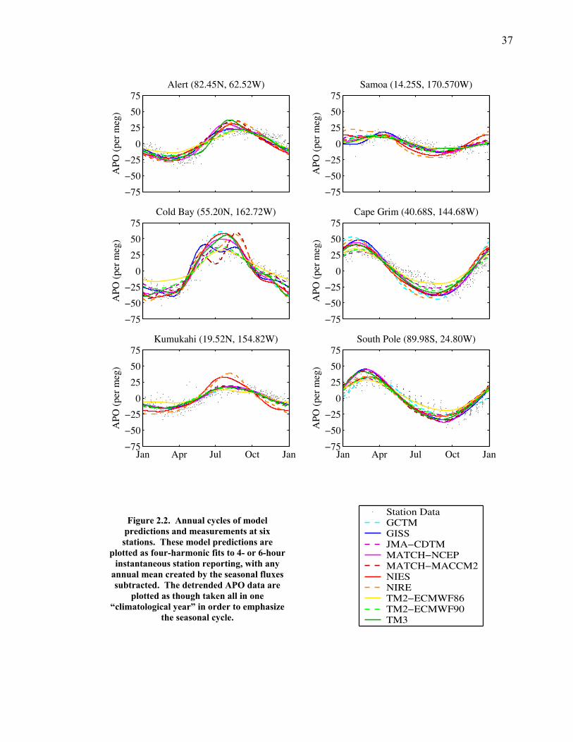
37
APO
(pe
r m
eg)
Alert (82.45N, 62.52W)
−75
−50
−25
0
25
50
75
APO
(pe
r m
eg)
Samoa (14.25S, 170.570W)
−75
−50
−25
0
25
50
75
APO
(pe
r m
eg)
Cold Bay (55.20N, 162.72W)
−75
−50
−25
0
25
50
75
APO
(pe
r m
eg)
Cape Grim (40.68S, 144.68W)
−75
−50
−25
0
25
50
75
APO
(pe
r m
eg)
Kumukahi (19.52N, 154.82W)
Jan Apr Jul Oct Jan−75
−50
−25
0
25
50
75
APO
(pe
r m
eg)
South Pole (89.98S, 24.80W)
Jan Apr Jul Oct Jan−75
−50
−25
0
25
50
75
Figure 2.2. Annual cycles of model predictions and measurements at six stations. These model predictions are
plotted as four-harmonic fits to 4- or 6-hour instantaneous station reporting, with any
annual mean created by the seasonal fluxes subtracted. The detrended APO data are
plotted as though taken all in one “climatological year” in order to emphasize
the seasonal cycle.
Station DataGCTMGISSJMA−CDTMMATCH−NCEPMATCH−MACCM2NIESNIRETM2−ECMWF86TM2−ECMWF90TM3
38
sinks, a result also found by Law et al. (1996). In tropical areas, the model predictions
of peak-to-peak amplitude generally cluster close to the measured values, whereas in
mid to high latitudes the model results span a two-fold range in predictions. Some
models show features that are not supported by the observations. For example, the
models MATCH-MACCM2 and NIRE show both double maxima and double minima
for Cold Bay, Alaska, and the model GISS shows a double peak. In contrast, the APO
data show a smooth annual cycle, though with increased variability in June and July.
Located on the edge of the North Pacific, Cold Bay is one of the more
challenging stations to fit because of its proximity to a large source/sink region in the
northern Pacific Ocean. While the global surface concentration maps (Figure 2.6,
discussed more in depth later) reveal broadly similar distributions with maximum
peak-to-peak amplitudes in the North Pacific, there are large differences in the
maximum and minimum concentrations and the horizontal extent of the peak.
Although it is not possible to identify which subgrid scale process is specifically
responsible, in some of the models APO mixes rapidly into the upper atmosphere,
leading to smaller annual cycles at lower levels of the atmosphere and larger annual
cycles at higher altitude, whereas reduced transport in other models results in large
annual cycles only in the proximity of the source. Such variability among model
predictions would likely occur for stations near the North Atlantic as well, but no
station data for oxygen exist from that area. Alert, the only station near the North
Atlantic, is too far north and most likely reflects a combination of North Pacific and
North Atlantic sources.
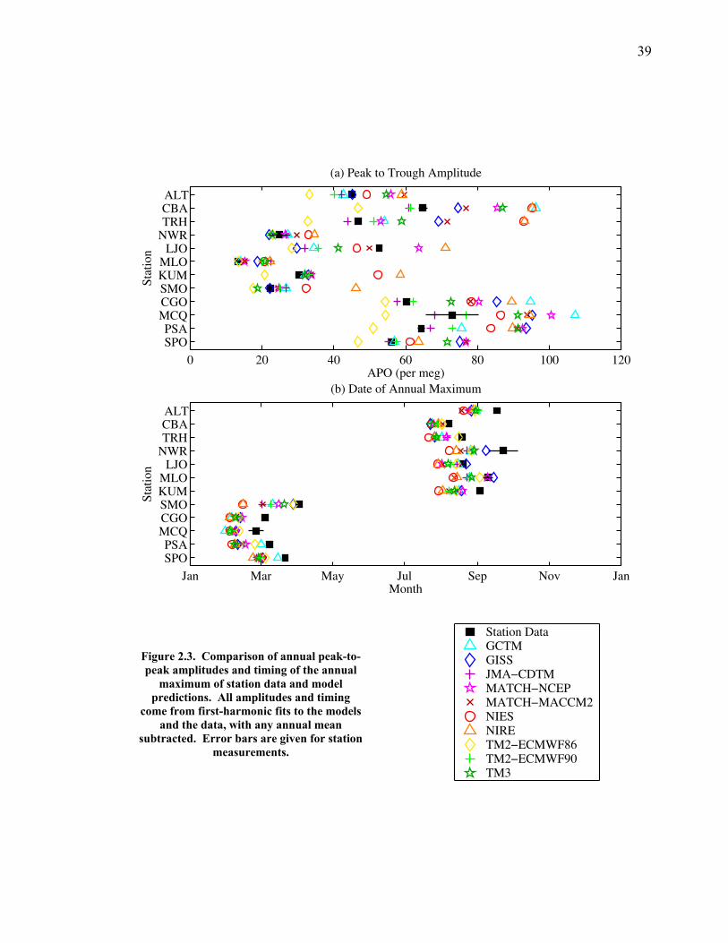
39
St
atio
n
(a) Peak to Trough Amplitude
APO (per meg)0 20 40 60 80 100 120
SPOPSA
MCQCGOSMOKUMMLOLJO
NWRTRHCBAALT
Stat
ion
(b) Date of Annual Maximum
MonthJan Mar May Jul Sep Nov Jan
SPOPSA
MCQCGOSMOKUMMLOLJO
NWRTRHCBAALT
Figure 2.3. Comparison of annual peak-to-peak amplitudes and timing of the annual
maximum of station data and model predictions. All amplitudes and timing
come from first-harmonic fits to the models and the data, with any annual mean
subtracted. Error bars are given for station measurements.
Station DataGCTMGISSJMA−CDTMMATCH−NCEPMATCH−MACCM2NIESNIRETM2−ECMWF86TM2−ECMWF90TM3
40
Comparisons of the annual peak-to-peak amplitude of the APO cycle and the
date of the annual maximum of each station are shown in Figure 2.3. For both the data
and the model predictions, I use first harmonic fits with the annual means subtracted.
Error bars for the fits to the station data are shown by black lines. Several of the
models fit the amplitude of the data well; others perform better in low latitude or high
latitude locations. Cape Grim and Macquarie Island have the largest spread in model
predictions of the annual cycle. Many of the models consistently overestimate the
annual cycle. This overestimation is also visible in the model cycles in Figure 2.2,
where rapid changes in model predictions of concentration do not match the more
gradual changes in the station data.
The model TM2-ECMWF86 underestimates the APO cycle at every station
and is an outlier among all the models. This model was chosen by Garcia and Keeling
(2001) to evaluate the estimates of the oxygen fluxes submitted as the input to this
study. As mentioned in the discussion of the flux fields, Garcia and Keeling (2001)
concluded that the Wanninkhof (1992) gas transfer velocity for O2 did not need to be
adjusted by a calibration factor.
At the Northern Hemisphere extratropical stations (Alert, Cold Bay, Trinidad
Head, and Niwot Ridge), the modeled amplitude is generally larger than the observed
amplitude. Weighing all stations and models equally, the models overestimate the
amplitude by a factor of 1.17. A similar analysis of the Southern Hemisphere stations
(Cape Grim, Macquarie Island, Palmer Station, and the South Pole) yields an
overestimate by a factor of 1.12. This rough calculation has many caveats, among
41
which is the assumption that the average of the models accurately predicts transport.
However, these results suggest that the initial Wanninkhof (1992) flux formulation
should be scaled by about 0.85, in contrast to Garcia and Keeling (2001) and Keeling
et al. (1998), who suggested a scaling constant of 1.15 in the Northern Hemisphere
and 1.23 in the Southern Hemisphere.
Based on known limitations of the flux fields, mentioned earlier, we expect the
model will predict cycles with phasing shifted early by about three weeks. As shown
in both Figures 2.2 and 2.3, the phasing of the model cycles is consistently shifted
early relative to observations on average by 20 days. This value is well-defined, as the
models agree closely on phasing.
La Jolla is underestimated by eight of the models. In order to avoid
contamination by local pollution sources, La Jolla is only sampled during steady west-
wind conditions, which are scarce during the fall and winter months. The seasonal
cycle estimated using the La Jolla station flask record may therefore be biased in
comparison to model predictions, which reflect a seasonal cycle regardless of wind
conditions (Keeling et al. 1998). However, another factor may be at play: the
meteorology of the California coast is dominated by a north-south coastal jet, which
may not be resolved in the coarse grids of the models (Burke and Thompson 1996;
Rogers et al. 1998). In contrast to La Jolla, the annual cycle at Trinidad Head station,
in northern California, tends to be overestimated by many of the models, similar to the
model predictions for stations even further north.
42
Data from Mauna Loa and from the South Pole, both high altitude stations, are
generally well-matched by model results, most likely because of the smaller annual
APO cycle at high altitudes far from oceanic sources and sinks where the flask
measurements are taken. Niwot Ridge, also a high latitude station, is the only
temperate continental station from the SIO network. Although there are only a few O2
and CO2 flask measurements from Niwot Ridge, all models are in close agreement on
the size of the annual cycle and agree well with the existing data. Although the cycle
is small, the reasonable fits suggest that models may more accurately represent values
over continents where the net flux is zero than those near sources and sinks of APO.
2.3.2 Station-station comparisons
As has been mentioned briefly in the previous section, stations near to oceanic
APO sources may be more challenging to model than those located far away from the
source regions. The stations for which APO data exist can generally be divided into
two groups: those in the proximity of source regions, such as Cold Bay or Cape Grim,
and those far away from source regions whether by altitude or horizontal distance,
such as Samoa, Mauna Loa, Niwot Ridge, or the South Pole.
The relationship between the concentrations at a station close to oceanic
sources and a distant station depends on the flux between them. Conceptually, their
relationship can be characterized by a simple two-box model according to:
( )DPtiP
P CCFQedt
dCV −−= ω (2.4)
43
( ),DPD
D CCFdt
dCV −= (2.5)
where C is the tracer concentration, subscripts P and D represent proximate and
distant stations respectively, Qeiωt is a sinusoidal forcing term describing air-sea flux,
F is the air flux between the two boxes, and V is the volume of each box. Both the air-
sea flux and the flux out of the box due to atmospheric transport are important for the
box close to sources; only the atmospheric transport is important for the box far away
from sources. The solutions to these equations are the following:
⎟⎟⎠
⎞⎜⎜⎝
⎛+⎟⎟
⎠
⎞⎜⎜⎝
⎛ +=
TOT
ti
D
DP Fi
QeVi
FViCωω
ω ω
and (2.6)
⎟⎟⎠
⎞⎜⎜⎝
⎛+
=TOT
ti
DD Fi
QeViFC
ωω
ω
, (2.7)
where ⎟⎟⎠
⎞⎜⎜⎝
⎛+=
DPTOT VV
FF 11 .
Treating the volumes of the boxes in terms of a relative change, the amplitude
ratio and phase difference between the boxes is thus dependent on a single,
dimensionless parameter, F*:
FVF Dω
=* . (2.8)
This model suggests a means of evaluating the station predictions from the TransCom
models. As discussed in the previous section, problems in the assumptions about
timing and the constants used to estimate air-sea oxygen fluxes may make direct
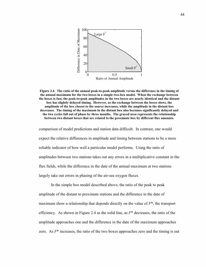
44
Ratio of Annual AmplitudeD
iffe
renc
e in
Dat
e of
Max
imum
Large F*
Small F*
0 0.5 10
20
40
60
80
100
Figure 2.4. The ratio of the annual peak-to-peak amplitude versus the difference in the timing of the annual maximum for the two boxes in a simple two-box model. When the exchange between
the boxes is fast, the peak-to-peak amplitudes in the two boxes are nearly identical and the distant box has slightly delayed timing. However, as the exchange between the boxes slows, the
amplitude of the box closest to the source increases, while the amplitude in the distant box decreases. The timing of the maximum in the distant box also becomes significantly delayed and
the two cycles fall out of phase by three months. The grayed area represents the relationship between two distant boxes that are related to the proximate box by different flux amounts.
comparison of model predictions and station data difficult. In contrast, one would
expect the relative differences in amplitude and timing between stations to be a more
reliable indicator of how well a particular model performs. Using the ratio of
amplitudes between two stations takes out any errors in a multiplicative constant in the
flux fields, while the difference in the date of the annual maximum at two stations
largely take out errors in phasing of the air-sea oxygen fluxes.
In the simple box model described above, the ratio of the peak to peak
amplitude of the distant to proximate stations and the difference in the date of
maximum show a relationship that depends directly on the value of F*, the transport
efficiency. As shown in Figure 2.4 as the solid line, as F* decreases, the ratio of the
amplitude approaches one and the difference in the date of the maximum approaches
zero. As F* increases, the ratio of the two boxes approaches zero and the timing is out
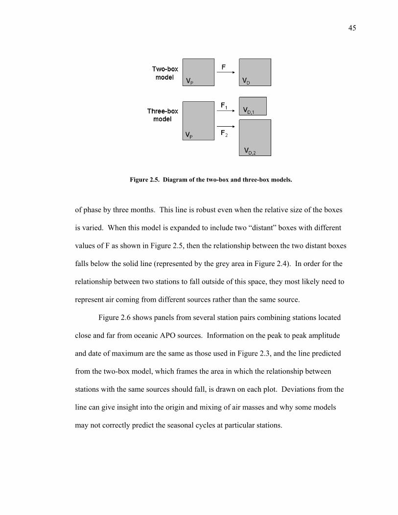
45
Figure 2.5. Diagram of the two-box and three-box models.
of phase by three months. This line is robust even when the relative size of the boxes
is varied. When this model is expanded to include two “distant” boxes with different
values of F as shown in Figure 2.5, then the relationship between the two distant boxes
falls below the solid line (represented by the grey area in Figure 2.4). In order for the
relationship between two stations to fall outside of this space, they most likely need to
represent air coming from different sources rather than the same source.
Figure 2.6 shows panels from several station pairs combining stations located
close and far from oceanic APO sources. Information on the peak to peak amplitude
and date of maximum are the same as those used in Figure 2.3, and the line predicted
from the two-box model, which frames the area in which the relationship between
stations with the same sources should fall, is drawn on each plot. Deviations from the
line can give insight into the origin and mixing of air masses and why some models
may not correctly predict the seasonal cycles at particular stations.
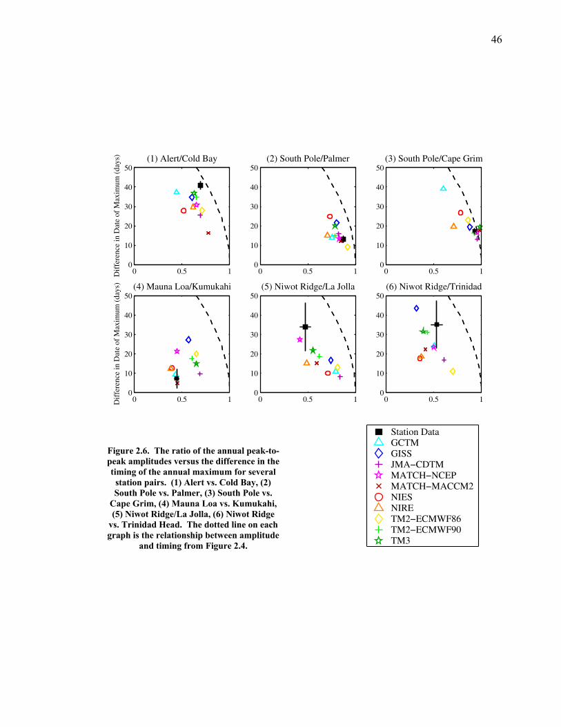
46
(1) Alert/Cold Bay
Dif
fere
nce
in D
ate
of M
axim
um (
days
)
0 0.5 10
10
20
30
40
50(2) South Pole/Palmer
0 0.5 10
10
20
30
40
50(3) South Pole/Cape Grim
0 0.5 10
10
20
30
40
50
(4) Mauna Loa/Kumukahi
Dif
fere
nce
in D
ate
of M
axim
um (
days
)
0 0.5 10
10
20
30
40
50(5) Niwot Ridge/La Jolla
0 0.5 10
10
20
30
40
50(6) Niwot Ridge/Trinidad
0 0.5 10
10
20
30
40
50
Figure 2.6. The ratio of the annual peak-to-peak amplitudes versus the difference in the timing of the annual maximum for several
station pairs. (1) Alert vs. Cold Bay, (2) South Pole vs. Palmer, (3) South Pole vs.
Cape Grim, (4) Mauna Loa vs. Kumukahi, (5) Niwot Ridge/La Jolla, (6) Niwot Ridge
vs. Trinidad Head. The dotted line on each graph is the relationship between amplitude
and timing from Figure 2.4.
Station DataGCTMGISSJMA−CDTMMATCH−NCEPMATCH−MACCM2NIESNIRETM2−ECMWF86TM2−ECMWF90TM3
47
Panels 1 and 2 in Figure 2.6 show Alert/Cold Bay and South Pole/Palmer, both
high-latitude pairs. The model predictions show greater spread in the Northern
Hemisphere than in the Southern Hemisphere, with a difference in the date of
maximum varying almost thirty days between models in the Northern Hemisphere
whereas the predictions scatter over less than twenty days in the Southern Hemisphere.
The South Pole and Palmer station are more tightly correlated, with station data and
model predictions falling closer to the area of the plot associated with a larger F value
representing greater exchange.
The South Pole/Palmer comparison as well as the South Pole/Cape Grim
comparison in Panel 3 suggests that mixing in models is more consistent in the
Southern Hemisphere than in the northern one. Air masses from around Palmer
Station and Cape Grim are exchanged more rapidly with air near the South Pole than
air masses are exchanged between Alert and Cold Bay. The South Pole and Cape
Grim in particular are closely linked as predictions and the station data tend to fall
along the line derived in the box model. The model predictions do not fall as closely
to the station results in Alert/Cold Bay, possibly reflecting the difference atmospheric
transport and mixing in the two hemispheres, as well as the heterogeneity in the
location of sources and sinks of APO in the Northern Hemisphere divided between the
Atlantic and Pacific Oceans. In the Southern Hemisphere, where sources are much
more evenly distributed, the model predictions fall relatively close to the station
results. In the Northern Hemisphere, the models tend to predict a maximum at Alert
that is earlier than the station data, whereas the models predict a slightly later
48
maximum at Cold Bay in comparison to data, as is confirmed by comparison with
Figure 2.2.
Panel 4 shows a comparison of the Mauna Loa and Kumukahi stations, both on
the big island of Hawaii. While Kumukahi is at sea level, the Mauna Loa station is at
3397 m. In the station flask data, the annual maximum at Kumukahi preceeds that at
Mauna Loa by about a week with amplitude ratio of about 0.5, which clearly put this
pair off of the line expected from mixing just between the two boxes. Keeling et al.
(1998) suggest that, while Mauna Loa may get part of its air from low latitude sources,
it may represent a mix of air from other sources with different phases. The model
predictions appear to fall in two different clusters: one which contains the actual
station data, and another, parallel cluster that is offset in both date of maximum and
the ratio. Keeling et al. (1998) suggest that the vertical gradient reflected in the
measurements at these stations may reflect a trade wind inversion at intermediate
altitudes that separates the air masses associated with the marine boundary layer from
those in the tropospheric air connected to the sinking Hadley’s circulation. This result
may show which models are better at predicting the mixing of the atmosphere at high
altitudes near the equator: GCTM, NIES, NIRE, and MATCH-MACCM2 all come
closer to describing the relationship between these two stations, whereas the other
model predictions fall on a different line.
Measurements at Niwot Ridge, as a mid-continental station, most likely
characterize a plume of air which has had its APO concentration determined by air-sea
exchange over the northeastern Pacific Ocean and which has mixed with other air
masses as it moves over the continent. Pair comparisons of Niwot Ridge against La
49
Jolla and Trinidad Head (Panels 5 and 6) both show that the models tend to
underpredict the timing difference between the coastal stations and Niwot Ridge and
overpredict the amplitude at Niwot Ridge relative to the coastal stations, suggesting
more effective transport in the models between the coasts and continental sites than is
reflected in measurements. Although most models keep the same relative position
between the two plots, the GISS model predictions have different relative positions;
GISS estimates a higher rate of exchange between La Jolla and Niwot Ridge than
between Trinidad and Niwot Ridge. This difference represents an idiosyncrasy of this
particular model.
2.3.3 Global surface patterns
Global maps of the peak-to-peak amplitude maps are shown for every model at
the surface level in Figure 2.7 and similar maps of the “rectifier” in Figure 2.8.
Following Law et al. (1996), the peak-to-peak amplitude is calculated as the difference
between the maximum and minimum monthly mean concentration at each grid point.
The “surface” level was defined by individual modelers and submitted independently
of the predictions at specific pressure levels. Similar patterns are visible across all the
models: the cycles over land, further from the locations of APO sources and sinks,
tend to be smaller with annual cycles of 60-70 per meg, whereas the cycles at the same
between the maximum and minimum monthly mean concentration at each grid point.
The “surface” level was defined by individual modelers and submitted independently
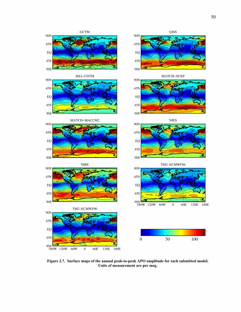
50
GCTM
90S
45S
EQ
45N
90NGISS
90S
45S
EQ
45N
90N
JMA−CDTM
90S
45S
EQ
45N
90NMATCH−NCEP
90S
45S
EQ
45N
90N
MATCH−MACCM2
90S
45S
EQ
45N
90NNIES
90S
45S
EQ
45N
90N
NIRE
90S
45S
EQ
45N
90NTM2−ECMWF86
180W 120W 60W 0 60E 120E 180E90S
45S
EQ
45N
90N
TM2−ECMWF90
180W 120W 60W 0 60E 120E 180E90S
45S
EQ
45N
90N
0 50 100
Figure 2.7. Surface maps of the annual peak-to-peak APO amplitude for each submitted model. Units of measurement are per meg.
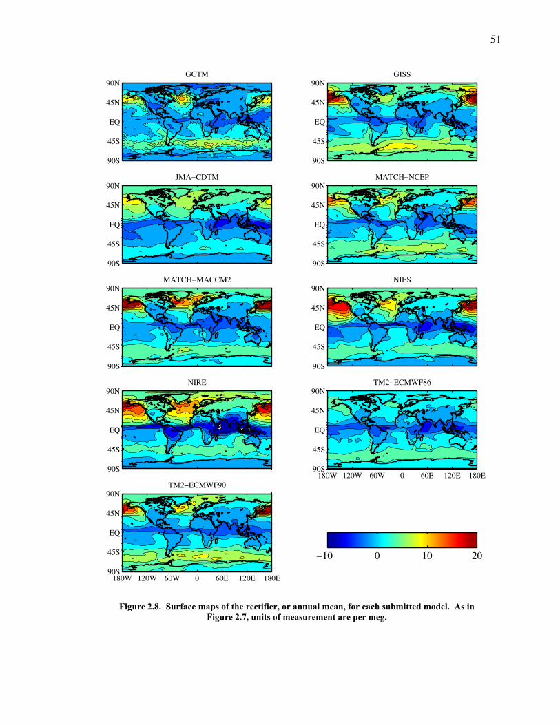
51
GCTM
90S
45S
EQ
45N
90NGISS
90S
45S
EQ
45N
90N
JMA−CDTM
90S
45S
EQ
45N
90NMATCH−NCEP
90S
45S
EQ
45N
90N
MATCH−MACCM2
90S
45S
EQ
45N
90NNIES
90S
45S
EQ
45N
90N
NIRE
90S
45S
EQ
45N
90NTM2−ECMWF86
180W 120W 60W 0 60E 120E 180E90S
45S
EQ
45N
90N
TM2−ECMWF90
180W 120W 60W 0 60E 120E 180E90S
45S
EQ
45N
90N
−10 0 10 20
Figure 2.8. Surface maps of the rectifier, or annual mean, for each submitted model. As in Figure 2.7, units of measurement are per meg.
52
of the predictions at specific pressure levels. Similar patterns are visible across all the
models: the cycles over land, further from the locations of APO sources and sinks,
tend to be smaller with annual cycles of 60-70 per meg, whereas the cycles at the same
latitudes over the ocean may be as high as 120 per meg in peak-to-peak amplitude. In
temperate latitudes, where the prevailing winds are from west to east, most models
show similar surface plots with small decreases in the size of the annual cycle across a
continent’s extent as an air mass gets more distant from the source area. Seasonal
cycles in APO over the ocean take 2-3 months to move across continents, spreading
out in both the north and south directions and getting damped over time. At the
western continental edges, even in Australia, contour lines in the peak-to-peak
amplitude go north (or dip south) in the Northern Hemisphere (or Southern
Hemisphere), following local wind patterns and isolating the largest cycles above the
oceans.
In general, the surface rectifier maps in Figure 2.8 look like the amplitude
maps: where the seasonal cycle is high, the rectifier value is also high. All the models
show a negative rectifier in equatorial areas, which can be 50% of the size of the
annual amplitude cycle; in contrast, the regions in the north Pacific and north Atlantic
located close to high source regions have a positive rectifier that is generally not larger
than 20% of the total cycle, and the surface rectifier over most of the ocean is close to
zero but slightly negative. In equatorial areas, the seasonality of the fluxes is small,
resulting in a small seasonal cycle of the atmospheric concentrations. The rectifier is
thus representing large changes in the seasonal transport in these areas, where deep
convection occurs around the Intertropical Convergence Zone (ITCZ). These results
53
suggest that equatorial areas may be a particularly difficult area for analysis of
atmospheric tracer measurements, as the signal is influenced by transport in both
hemispheres that can change significantly in strength on a seasonal basis. Most
general circulation models are also known to have problems representing the seasonal
migration of the ITCZ precipitation (Gates et al. 1999; Hack et al. 1998; Wu et al.
2003); in CCM3, the ITCZ precipitation peak remains north of the equator throughout
the year (Wu et al. 2003). The seasonal amplitude and rectifier predictions in this area
of tracer transport models which rely on output of general circulation models for their
winds may be particularly suspect.
2.3.4 Zonal patterns
Figures 2.9-2.12 compare model predictions of altitudinal zonal averages. The
variables are first calculated for each grid point, then averaged using a given model’s
zonal resolution. All the models agree qualitatively in their large-scale patterns of the
seasonal cycle: near the surface, the largest annual amplitudes in the latitudinal means
are in the Southern Ocean at about 60oS and a smaller peak occurs at 45-60oN. The
profiles in Figure 2.9 show a more tightly defined peak in the Southern Hemisphere
than in the Northern Hemisphere during the summer months (February and August,
respectively), reflecting the narrower zonal distribution of source regions in the
Southern Hemisphere. Figure 2.10 presents zonal mean transects for every model
rather than profiles, showing that the zonal mean amplitude at the surface increases
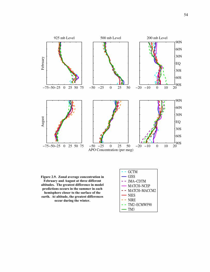
54
Febr
uary
925 mb Level
−75−50−25 0 25 50 75
500 mb Level
−50 −25 0 25 50
200 mb Level
−20 −10 0 10 2090S
60S
30S
EQ
30N
60N
90NA
ugus
t
−75−50−25 0 25 50 75APO Concentration (per meg)−50 −25 0 25 50 −20 −10 0 10 20
90S
60S
30S
EQ
30N
60N
90N
Figure 2.9. Zonal average concentration in February and August at three different
altitudes. The greatest difference in model predictions occurs in the summer in each
hemisphere closer to the surface of the earth. At altitude, the greatest differences
occur during the winter.
GCTMGISSJMA−CDTMMATCH−NCEPMATCH−MACCM2NIESNIRETM2−ECMWF90TM3
55
from 5-20 per meg at the equator to 40-70 per meg at 45-60oN and 70-100 per meg at
60oS. Away from the source regions, the variation between models is smaller, a
pattern which was found in studies of land sources of CO2 (Law et al. 1996).
Many of the differences in annual amplitude between models are attenuated at
500 mb but emerge again at 200 mb, where the maximum in each hemisphere shifts
slightly poleward at higher altitudes. Near the top of the atmosphere, the annual
cycles are small, and the models show much more variability, agreeing closely at the
equator where the amplitude is near zero but predicting very different annual
amplitudes at the poles. This variability among models generally comes from
differences between models during a particular season; for example, at 200 mb, the
models agree quite closely in February in the Southern Hemisphere with the exception
of one outlier (TM2-ECMWF90) (shown in Figure 2.9). However, the model
predictions differ by almost 15 per meg for the month of August, and it is these
differences that lead to differences between the models in the predicted amplitude. At
the same altitude in the Northern Hemisphere, the greatest discrepancy in the model
predictions occurs in February rather than August. It is thus the wintertime
concentrations at high altitude (close to the tropopause) that show the most divergence
between models, at the times that a polar vortex is strongest and atmospheric patterns
may be more difficult to represent in a model. Some of the models do not have a
stratosphere, and so any predictions near this level are suspect.
In contrast, at 500 mb and 925 mb, the largest discrepancy between models
occurs in high latitudes during the summer, rather than during the winter. The zonal
averages in Figure 2.9 obscure the relevant spatial patterns visible in the surface maps
56
of Figure 2.7; the largest cycles are actually correlated with the sources and sinks of
APO in the northern Pacific and Atlantic Oceans, but the overall mean for that latitude
in the Northern Hemisphere is smaller than in the Southern Ocean because the oceanic
areas are interspersed with land masses. The differences between models representing
large source regions helps explain the difference in summer peaks. However, vertical
transport is also strongest in the summertime over continents as the land warms up
faster than the overlying air, and differences in how vertical transport is modeled can
cause discrepancies in the predictions.
Figure 2.11 shows mean zonal transects of the rectifier. At the surface, the
rectifier patterns seem primarily driven by the size of the local seasonal air-sea flux.
Away from the surface near the equator, where warm and moist air is rising in the
upward branch of the Hadley cells, the values are negative at all but the highest
altitudes. Several models also show positive values at middle and high altitudes in
areas near the downward branches of the Hadley cell at about 30o in each hemisphere.
This is as expected; where the atmosphere has significant uplift, the rectifier should be
negative, and where the atmosphere is descending, the rectifier should be positive.
Large rectifier values extend high into the atmosphere over the Northern Hemisphere,
whereas they are more limited to the surface in the Southern Hemisphere. This
observation is most likely due to the strength of summertime vertical transport over
continents and the fact that the Northern Hemisphere has a much greater land mass.
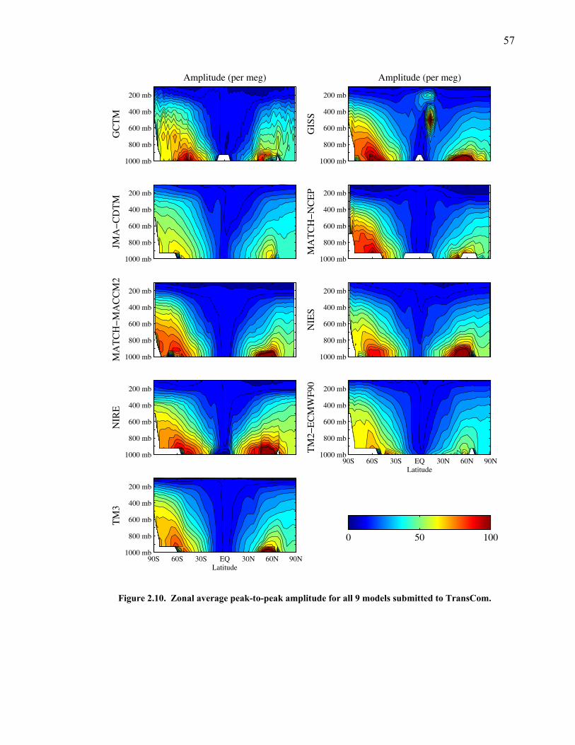
57
GC
TM
Amplitude (per meg)
1000 mb
800 mb
600 mb
400 mb
200 mb
GIS
S
Amplitude (per meg)
1000 mb
800 mb
600 mb
400 mb
200 mb
JMA−
CD
TM
1000 mb
800 mb
600 mb
400 mb
200 mb
MA
TC
H−
NC
EP
1000 mb
800 mb
600 mb
400 mb
200 mb
MA
TC
H−
MA
CC
M2
1000 mb
800 mb
600 mb
400 mb
200 mb
NIE
S
1000 mb
800 mb
600 mb
400 mb
200 mb
NIR
E
1000 mb
800 mb
600 mb
400 mb
200 mb
TM
2−E
CM
WF9
0
Latitude90S 60S 30S EQ 30N 60N 90N
1000 mb
800 mb
600 mb
400 mb
200 mb
TM
3
Latitude90S 60S 30S EQ 30N 60N 90N
1000 mb
800 mb
600 mb
400 mb
200 mb
0 50 100
Figure 2.10. Zonal average peak-to-peak amplitude for all 9 models submitted to TransCom.
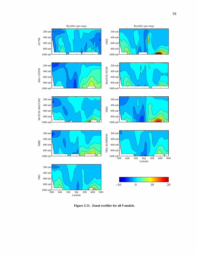
58
GC
TM
Rectifier (per meg)
1000 mb
800 mb
600 mb
400 mb
200 mb
GIS
S
Rectifier (per meg)
1000 mb
800 mb
600 mb
400 mb
200 mb
JMA−
CD
TM
1000 mb
800 mb
600 mb
400 mb
200 mb
MA
TC
H−
NC
EP
1000 mb
800 mb
600 mb
400 mb
200 mb
MA
TC
H−
MA
CC
M2
1000 mb
800 mb
600 mb
400 mb
200 mb
NIE
S
1000 mb
800 mb
600 mb
400 mb
200 mb
NIR
E
1000 mb
800 mb
600 mb
400 mb
200 mb
TM
2−E
CM
WF9
0
Latitude90S 60S 30S EQ 30N 60N 90N
1000 mb
800 mb
600 mb
400 mb
200 mb
TM
3
Latitude90S 60S 30S EQ 30N 60N 90N
1000 mb
800 mb
600 mb
400 mb
200 mb
−10 0 10 20
Figure 2.11. Zonal rectifier for all 9 models.
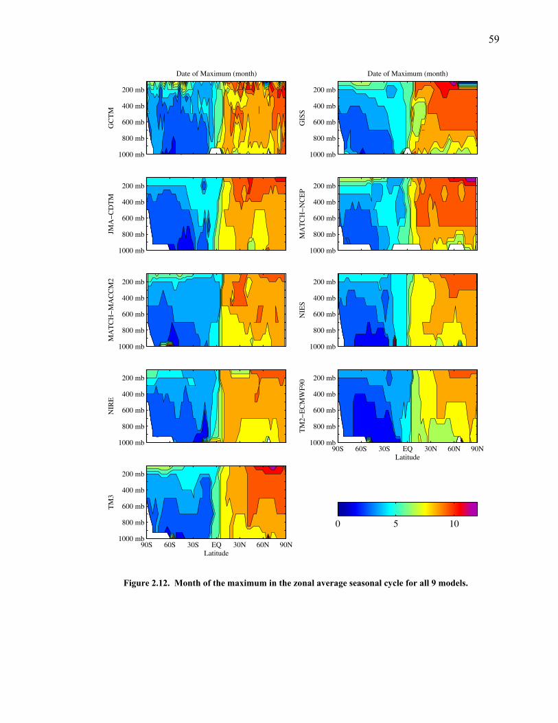
59
GC
TM
Date of Maximum (month)
1000 mb
800 mb
600 mb
400 mb
200 mb
GIS
S
Date of Maximum (month)
1000 mb
800 mb
600 mb
400 mb
200 mb
JMA−
CD
TM
1000 mb
800 mb
600 mb
400 mb
200 mb
MA
TC
H−
NC
EP
1000 mb
800 mb
600 mb
400 mb
200 mb
MA
TC
H−
MA
CC
M2
1000 mb
800 mb
600 mb
400 mb
200 mb
NIE
S
1000 mb
800 mb
600 mb
400 mb
200 mb
NIR
E
1000 mb
800 mb
600 mb
400 mb
200 mb
TM
2−E
CM
WF9
0
Latitude90S 60S 30S EQ 30N 60N 90N
1000 mb
800 mb
600 mb
400 mb
200 mb
TM
3
Latitude90S 60S 30S EQ 30N 60N 90N
1000 mb
800 mb
600 mb
400 mb
200 mb
0 5 10
Figure 2.12. Month of the maximum in the zonal average seasonal cycle for all 9 models.
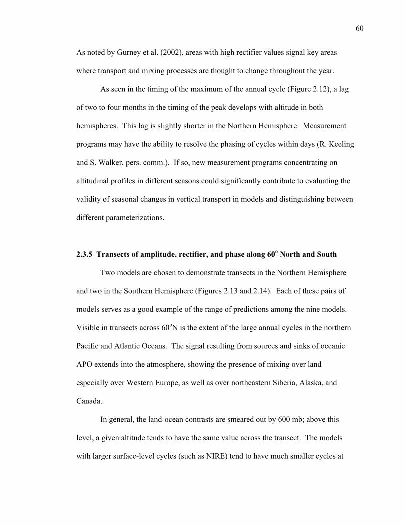
60
As noted by Gurney et al. (2002), areas with high rectifier values signal key areas
where transport and mixing processes are thought to change throughout the year.
As seen in the timing of the maximum of the annual cycle (Figure 2.12), a lag
of two to four months in the timing of the peak develops with altitude in both
hemispheres. This lag is slightly shorter in the Northern Hemisphere. Measurement
programs may have the ability to resolve the phasing of cycles within days (R. Keeling
and S. Walker, pers. comm.). If so, new measurement programs concentrating on
altitudinal profiles in different seasons could significantly contribute to evaluating the
validity of seasonal changes in vertical transport in models and distinguishing between
different parameterizations.
2.3.5 Transects of amplitude, rectifier, and phase along 60o North and South
Two models are chosen to demonstrate transects in the Northern Hemisphere
and two in the Southern Hemisphere (Figures 2.13 and 2.14). Each of these pairs of
models serves as a good example of the range of predictions among the nine models.
Visible in transects across 60oN is the extent of the large annual cycles in the northern
Pacific and Atlantic Oceans. The signal resulting from sources and sinks of oceanic
APO extends into the atmosphere, showing the presence of mixing over land
especially over Western Europe, as well as over northeastern Siberia, Alaska, and
Canada.
In general, the land-ocean contrasts are smeared out by 600 mb; above this
level, a given altitude tends to have the same value across the transect. The models
with larger surface-level cycles (such as NIRE) tend to have much smaller cycles at
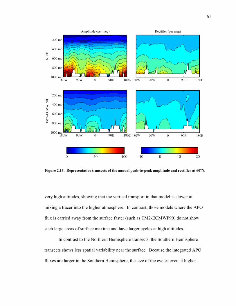
61
NIR
E
Amplitude (per meg)
180W 90W 0 90E 180E1000 mb
800 mb
600 mb
400 mb
200 mb
TM
2−E
CM
WF9
0
180W 90W 0 90E 180E1000 mb
800 mb
600 mb
400 mb
200 mb
Rectifier (per meg)
180W 90W 0 90E 180E
180W 90W 0 90E 180E
0 50 100 −10 0 10 20
Figure 2.13. Representative transects of the annual peak-to-peak amplitude and rectifier at 60oN.
very high altitudes, showing that the vertical transport in that model is slower at
mixing a tracer into the higher atmosphere. In contrast, those models where the APO
flux is carried away from the surface faster (such as TM2-ECMWF90) do not show
such large areas of surface maxima and have larger cycles at high altitudes.
In contrast to the Northern Hemisphere transects, the Southern Hemisphere
transects shows less spatial variability near the surface. Because the integrated APO
fluxes are larger in the Southern Hemisphere, the size of the cycles even at higher
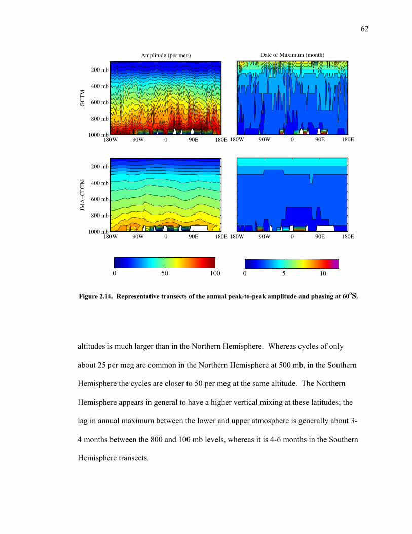
62
GC
TM
Amplitude (per meg)
180W 90W 0 90E 180E1000 mb
800 mb
600 mb
400 mb
200 mb
JMA−
CD
TM
180W 90W 0 90E 180E1000 mb
800 mb
600 mb
400 mb
200 mb
Date of Maximum (month)
180W 90W 0 90E 180E
180W 90W 0 90E 180E
0 50 100 0 5 10
Figure 2.14. Representative transects of the annual peak-to-peak amplitude and phasing at 60oS.
altitudes is much larger than in the Northern Hemisphere. Whereas cycles of only
about 25 per meg are common in the Northern Hemisphere at 500 mb, in the Southern
Hemisphere the cycles are closer to 50 per meg at the same altitude. The Northern
Hemisphere appears in general to have a higher vertical mixing at these latitudes; the
lag in annual maximum between the lower and upper atmosphere is generally about 3-
4 months between the 800 and 100 mb levels, whereas it is 4-6 months in the Southern
Hemisphere transects.
63
2.4 Discussion
Plots of model transects can be used to classify the models into groups with
stronger and weaker vertical transport, as found by Denning et al. (1999). The
gradients in zonal mean peak-to-peak amplitude over source regions in the extratropics
of the Southern Hemisphere, visible in Figure 2.10, are used to roughly group models
with stronger or weaker vertical transport. Those with stronger vertical transport are
JMA-CDTM, NIES, TM2-ECMWF90, and TM3. Those with weaker mixing and
larger gradients include GCTM, MATCH-NCEP, MATCH-MACCM2, and to a lesser
extent, GISS and NIRE. This grouping has TM3 and GISS classed differently than in
Denning et al. (1999), possibly due to changes in the models used and/or differences
in tracer characteristics that necessitate different classification schemes. Those with
weaker mixing significantly overestimate the station amplitudes shown in Figure 2.3
in the Southern Hemisphere and at mid-latitudes in the Northern Hemisphere, as more
APO tends to accumulate at lower altitudes rather than being mixed aloft in the
atmosphere. However, no high-altitude data exist to compare with the altitudinal
profiles predicted by different models.
Beyond an understanding of how each model performs relative to the other
models, these APO model calculations are important for suggesting new locations
where it may be helpful to have oxygen and carbon dioxide measurements to test the
existing models and help pinpoint areas in which models need to be improved. For
example, whether parameterizations of stronger or weaker vertical mixing are more
appropriate could be tested by measurements from vertical profiles in the Southern
Hemisphere and at mid-latitudes in the Northern Hemisphere. Because the difference
64
between models at lower altitudes (950 – 500 mb) in the extra-tropics is greatest in the
summer, particular attention should be paid to measurements in the Northern
Hemisphere during July – September and in the Southern Hemisphere during January
- March.
The Southern Hemisphere can probably be well-described with a zonal array of
stations without the need for a longitudinal array. Because of the heterogeneity of
land and sea masses in the Northern Hemisphere compared to the Southern
Hemisphere, measurement locations spread across different longitudes as well as
different latitudes is more important. Horizontal transport can be tested by more
measurements in close proximity to areas of large sources and sinks in the Northern
Hemisphere; at the present time, at least some stations exist near the large source
region in the northern Pacific Ocean although more could be useful. However, no
measurements exist in the region of the large source in the northern Atlantic Ocean, a
situation that should be rectified by placing stations in eastern Canada and in the
British Isles.
Another need is for more land-based stations, especially over the large
northern hemispheric continents of Eurasia and North America. Measurements over
land, where the net sources and sinks of APO are zero and atmospheric transport can
be better isolated, may be significant in evaluating different model parameterizations.
Here, seasonal information is important in observing how seasonal cycles in air-sea
flux fields propagate over large, mid-latitude continents where no sources or sinks
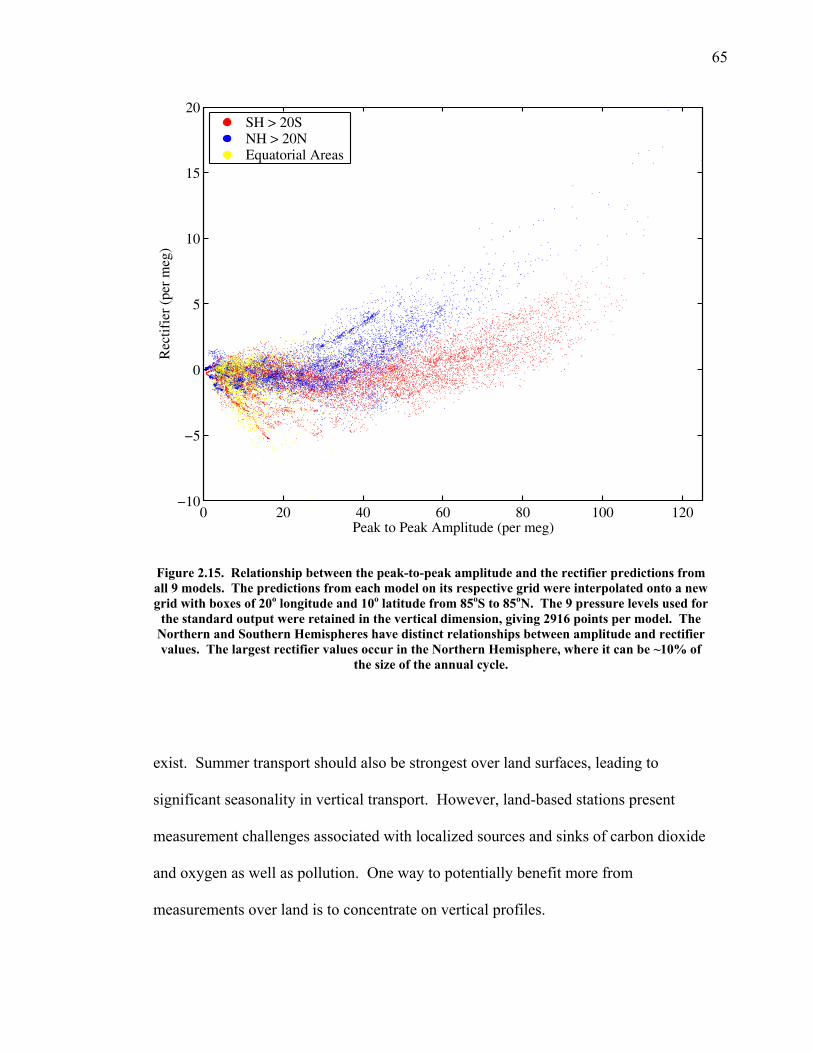
65
Peak to Peak Amplitude (per meg)
Rec
tifie
r (p
er m
eg)
0 20 40 60 80 100 120−10
−5
0
5
10
15
20SH > 20SNH > 20NEquatorial Areas
Figure 2.15. Relationship between the peak-to-peak amplitude and the rectifier predictions from all 9 models. The predictions from each model on its respective grid were interpolated onto a new grid with boxes of 20o longitude and 10o latitude from 85oS to 85oN. The 9 pressure levels used for
the standard output were retained in the vertical dimension, giving 2916 points per model. The Northern and Southern Hemispheres have distinct relationships between amplitude and rectifier values. The largest rectifier values occur in the Northern Hemisphere, where it can be ~10% of
the size of the annual cycle.
exist. Summer transport should also be strongest over land surfaces, leading to
significant seasonality in vertical transport. However, land-based stations present
measurement challenges associated with localized sources and sinks of carbon dioxide
and oxygen as well as pollution. One way to potentially benefit more from
measurements over land is to concentrate on vertical profiles.
66
The rectifiers predicted by models at different stations are correlated with the
overall peak-to-peak amplitude of the seasonal cycle. As demonstrated in Figure 2.15,
where the cycle is small (less than 20 per meg), the rectifier tends to be close to zero
or negative. Above this value, the Southern and Northern Hemispheres have different
patterns in all the models: the Northern Hemisphere tends to have larger values of the
rectifier than the Southern Hemisphere for the same size amplitude. This result most
likely stems from the heterogeneity of land and ocean masses in the Northern
Hemisphere. Besides leading to a more complex spatial distribution of sources and
sinks, this heterogeneity most likely also leads to a more complex seasonal change in
transport due to the effect of heating and cooling on continents as well as seasonal
changes above the ocean. In the Southern Hemisphere, among all the models the
rectifier effect never is larger than about 7 per meg; in the Northern Hemisphere, the
value climbs to 15 per meg at its highest. Also, in the Southern Hemisphere the
rectifier value stays close to zero until the seasonal amplitude climbs above 60 per
meg; in the Northern Hemisphere, the rectifier starts increasing in concert with the
amplitude at about 30 per meg. It is hoped that these model predictions provide a
bound on the size of the rectifier resulting from the interaction of the seasonal
component in atmospheric transport and tracer fields.
67
2.5 Conclusions
Through comparison with station APO data, I evaluated the effectiveness of
the atmospheric transport models submitted to the TransCom project in modeling a
tracer with only oceanic fluxes. Overall, the models correctly predicted the general
large-scale surface patterns of APO and the seasonal cycle as compared to APO data
from eleven different stations. Some problems with the models have also been
highlighted by this comparison. These results are dependent on the accuracy of the
initial O2 and N2 air-sea flux estimates. However, these results may aid in
understanding model predictions and constraints when estimating other variables.
Global maps of the rectifier effect may help identify areas where atmospheric
measurements can be considered independently on seasonal time scales and annual
averages. In equatorial areas, such an analysis may be very problematic given the
small size of annual cycles of many species. The rectifier effect is also larger in the
Northern Hemisphere than in the Southern Hemisphere, suggesting that the mean and
seasonal signals are less independent in the Northern Hemisphere.
In general, the predictions of the TransCom models show more variability
between models in the Northern Hemisphere than in the Southern Hemisphere.
Sources and sinks of air-sea gas flux have a heterogeneous distribution because of the
distribution of continents, leading to larger localized seasonal cycles in the
atmospheric concentration of APO and large land masses over which APO is carried
passively. Because westward winds are generally weaker in the Northern Hemisphere
(Peixoto and Oort 1992), a zonal band may not mix as fast in the Northern
68
Hemisphere as in the Southern Hemisphere, leading to greater east-west heterogeneity
of concentrations in the lower atmosphere and larger differences in phase.
The results of maps of model predictions suggest that more stations distributed
within a particular latitude band would be helpful to test models in the Northern
Hemisphere, whereas zonally distributed stations are probably adequate to represent
the Southern Hemisphere. Critical areas include the North Atlantic as well as the
North Pacific, where models show the greatest disparity in predictions. In these
localized areas of sources and sinks, the models show significant variability in
describing how these fluxes are transported both horizontally and vertically, and more
stations may help to distinguish between different methods of modeling horizontal
transport.
Also important are more profiles at altitude, especially in different seasons, as
the strength of vertical transport is critical to determining surface patterns. At the
present time, it is difficult to test parameterizations of vertical transport solely with
monitoring stations at the sea surface. Measurements at different altitudes could
resolve differences in atmospheric concentration and phase, helping to understand
seasonal differences in vertical transport. Such profiling has rarely been performed
because of the expense and the difficulty of repeating such measurements in different
seasons. However, these profiles may be necessary to distinguish between different
parameterizations of vertical transport and to continue to improve atmospheric
transport models.
69
2.6 Bibliography Battle, M., S. M. Fletcher, M. Bender, R. Keeling, N. Gruber, P. P. Tans, M. B.
Hendricks, D. T. Ho, C. Simonds, R. Mika, A. C. Manning, and B. Paplawsky. 2005. New observational constraints on atmospheric and oceanic models of the oxygen and carbon dioxide cycles, in preparation.
Bousquet, P., P. Ciais, P. Peylin, M. Ramonet, and P. Monfray. 1999. Inverse
modeling of annual atmospheric CO2 sources and sinks: 1. Method and control inversion. J. Geophys. Res. 104: 26,161-26,178.
Burk, S. D. and W. T. Thompson. 1996. The summertime low level jet and marine
boundary layer structure along the California coast. Mon. Weather Rev. 124: 668-686.
Denning, A. S., I. Y. Fung, and D. Randall. 1995. Latitudinal gradient of atmospheric
CO2 due to seasonal exchange with land biota. Nature 376: 240-243. Denning, A. S., M. Holzer, K. R. Gurney, M. Heimann, R. M. Law, P. J. Rayner, I. Y.
Fung, S-M. Fan, S. Taguchi, P. Friedlinstein, Y. Balkanski, J. Tayler, M. Maiss, and I. Levin. 1999. Three-dimensional transport and concentration of SF6: A model intercomparison study (Transcom 2). Tellus 51B: 266-297.
Garcia, H. E. and R. F. Keeling. 2001. On the global oxygen anomaly and air-sea
flux. J. Geophys. Res. 106: 31,155-31,166. Gates, W. L., J. S. Boyle, C. Covey, C. G. Dease, C. M. Doutriaux, R. S. Drach, M.
Florino, P. J. Gleckler, J. J. Hnilo, S. M. Marlais, T. J. Phillips, G. L. Potter, B. D. Santer, K. R. Sperber, K. E. Taylor, and D. N. Williams. 1999. An overview of the results of the atmospheric model intercomparison project (AMIP I). Bull. Am. Meteorol. Soc. 81: 29-55.
Gibson, J. K., P. Kallberg, S. Uppala, A. Hernandez, A. Nomura, and E. Serrano.
1997. ERA description, ECMWF Re-Analysis Project Report Series 1, 72 pp. European Center for Medium-Range Weather Forecasts. Reading, England, U.K.
Glueckauf, E. 1951. The composition of atmospheric air. Compendium of
Meteorology. Am. Met. Soc. Boston, 3-11. Gruber, N., M. Gloor, S-M. Fan, and J. L. Sarmiento. 2001. Air-sea flux of oxygen
estimated from bulk data: Implications for the marine and atmospheric oxygen cycles. Glob. Biogeochem. Cycles 15(4): 783-803.
70
Gurney, K. R., R. M. Law, A. S. Denning, P. J. Rayner, D. Baker, P. Bousquet, L. Bruhwiler, Y-H. Chen, P. Ciais, S-M. Fan, I. Y. Fung, M. Gloor, M. Heimann, K. Higuchi, J. John, T. Maki, S. Maksyutov, K. Masarie, P. Peylin, M. Prather, B. Pak, J. Randerson, J. Sarmiento, S. Taguchi, T. Takahashi, and C-W. Yuen. 2002. Towards robust regional estimates of CO2 sources and sinks using atmospheric transport models. Nature 415: 626-630.
Gurney, K. R., R. M. Law, A. S. Denning, P. J. Rayner, D. Baker, P. Bousquet, L.
Bruhwiler, Y-H. Chen, P. Ciais, S-M. Fan, I. Y. Fung, M. Gloor, M. Heimann, K. Higuchi, J. John, E. Kowalczyk, T. Maki, S. Maksyutov, P. Peylin, M. Prather, B. Pak, J. Sarmiento, S. Taguchi, T. Takahashi, and C-W. Yuen. 2003. Transcom 3 inversion intercomparison: 1. Annual mean control results and sensitivity to transport and prior flux information. Tellus 55B: 555-579.
Gurney, K. R., R. M. Law, A. S. Denning, P. J. Rayner, B. C. Pak, D. Baker, P.
Bousquet, L. Bruhwiler, Y-H. Chen, P. Ciais, I. Y. Fung, M. Heimann, J. John, T. Maki, S. Maksyutov, P. Peylin, M. Prather, and S. Taguchi. 2004. Transcom 3 inversion intercomparison: Model mean results for the estimation of seasonal carbon sources and sinks. Glob. Biogeochem. Cycles 18, GB1010 (doi: 10.1029/2003GB002111).
Hack, J. J., J. T. Kiehl, and J. W. Hurrell. 1998. The hydrologic and thermodynamic
characteristics of the NCAR CCM3. J. Clim. 11: 1179-1206. Hansen, J., Mki Sato, R. Ruedy, A. Lacis, K. Asamoah, and coauthors. 1997.
Forcings and chaos in interannual to decadal climate change. J. Geophys. Res. 102: 25,679-25,720.
Heimann, M. 1995. The global atmospheric tracer model TM2. Technical Report 10.
Deutsches Klimarechenzentrum, Hamburg, Germany, 51 pp. Heimann, M., and C. D. Keeling. 1989. A three-dimensional model of atmospheric
CO2 transport based on observed winds, 2: Model description and simulated tracer experiments. In: Peterson, D. H., ed. Aspects of Climate Variability in the Pacific and Western Americas, Geophysics. Monograph Series, Vol. 55. American Geophysical Union: Washington, D.C.
Houghton, J. T., Y. Ding, D. J. Griggs, M. Noguer, P. J. van der Linden, X. Dai, K.
Maskell, and C. A. Johnson (eds). 2001. Climate Change 2001: The Scientific Basis (Contribution of Working Group I to the Third Assessment Report of the Intergovernmental Panel on Climate Change). Cambridge University Press: Cambridge, U.K., and New York, U.S.A.
71
Iwasaki, T., T. Maki, and K. Katayama. 1998. Tracer transport model at Japan Meteorological Agency and its application to the ETEX data. Atmos. Environ. 32: 4285-4295.
Keeling, R. F. 1988. Development of an interferometric oxygen analyzer for precise
measurement of the atmospheric O2 mole fraction. Ph.D. thesis: Harvard University, Cambridge, MA.
Keeling, R. F., R. P. Najjar, M. L. Bender, and P. P. Tans. 1993. What atmospheric
oxygen measurements can tell us about the global carbon cycle. Glob. Biogeochem. Cycles 7: 37-67.
Keeling, R. F., B. B. Stephens, R. G. Najjar, S. C. Doney, D. Archer, and M.
Heimann. 1998. Seasonal variations in the atmospheric O2/N2 ratio in relation to kinetics of air-sea gas exchange. Glob. Biogeochem. Cycles 12: 141-163.
Law, R. M. and P. J. Rayner. 1999. Impacts of seasonal covariance on CO2
inversions. Glob. Biogeochem. Cycles 13: 845-856. Law, R. M., P. J. Rayner, A. S. Denning, D. Erickson, I. Y. Fung, M. Heimann, S. C.
Piper, M. Ramonet, S. Taguchi, J. A. Taylor, C. M. Trudinger, and I. G. Watterson. 1996. Variations in modeled atmospheric transport of carbon dioxide and the consequences for CO2 inversions. Glob. Biogeoch. Cycles 10: 783-796.
Law, R. M., Y-H. Chen, K. R. Gurney, and Transcom 3 Modellers. 2003. Transcom
3 CO2 inversion intercomparison: 2. Sensitivity of annual mean results to data choices. Tellus 55B: 580-595.
Levy, H., J. D. Mahlman, and W. J. Moxim. 1982. Tropospheric N2O variability. J.
Geophys. Res. 87: 3061-3080. Liss, P. S. and L. Merlivat. 1986. Air-sea gas exchange rates: introduction and
synthesis. Pages 113-127 in: P. Buat-Ménard (ed.). The Role of Air-Sea Exchange in Geochemical Cycling. D. Reidel Publishing Co.: Norwell, Mass.
Lueker, T. J, S. J. Walker, M. K. Vollmer, R. F. Keeling, C. D. Nevison, and R. F.
Weiss. 2003. Coastal upwelling air-sea fluxes revealed in atmospheric observations of O2/N2, CO2, and N2O. Geophys. Res. Lett. 30 (doi: 10.1029/2002GL016615).
Mahlman, J. D. and W. J Moxim. 1978. Tracer simulation using a global general
circulation model: results from a mid-latitude instantaneous source experiment. J. Atmos. Sci. 35: 1340-1374.
72
Maksyutov, S. and G. Inoue. 2000. Vertical profiles of radon and CO2 simulated by the global atmospheric transport model. In: CGER report, CGER-I039-2000, CGER, NIES, Japan, v. 7, 39-41.
Manning, Andrew C. 2001. Temporal variability of atmospheric oxygen from both
continuous measurements and a flask sampling network: Tools for studying the global carbon cycle. Ph.D. thesis: University of California, San Diego.
Najjar, R. G. and R. F. Keeling. 1997. Analysis of the mean annual cycle of the
dissolved oxygen anomaly in the World Ocean. J. Mar. Res. 55: 117-151. Najjar, R. G. and R. F. Keeling. 2000. Mean annual cycle of the air-sea oxygen flux:
A global view. Glob. Biogeochem. Cycles 14: 573-584. Rasch, P., N. M. Mahowald, and B. E. Eaton. 1997. Representations of transport,
convection and the hydrological cycles in chemical transport models: Implications for the modeling of short lived and soluble species. J. Geophys. Res. 102: 28,127-28,138.
Rogers, D. P., C. E. Dorman, K. A. Edwards, I. M. Brooks, W. K. Melville, S. D.
Burk, W. T. Thompson, T. Holt, L. M. Strom, M. Tjernstrom, B. Grisogono, J. M. Bane, W. A. Nuss, B. M. Morley, and A. J. Schanot. 1998. Highlights of Coastal Waves 1996. Bull. Am. Meteorol. Soc. 79: 1307-1326.
Severinghaus, J. P. 1995. Studies of the terrestrial O2 and carbon cycles in sand dune
gases and in Biosphere 2. Ph.D. thesis: Columbia University, New York. Shea, D. J., K. E. Trenberth, and R. W. Reynolds. 1992. A global monthly sea
surface temperature climatology. J. Clim. 5: 987-1001. Stephens, B. B., R. F. Keeling, M. Heimann, K. D. Six, R. Murnane, and K. Caldiera.
1998. Testing global ocean carbon cycle models using measurements of atmospheric O2 and CO2 concentration. Glob. Biogeochem. Cycles 12: 213-230.
Taguchi, S. 1996. A three-dimensional model of atmospheric CO2 transport based on
analyzed winds: Model description and simulation results for TRANSCOM. J. Geophys. Res. 101: 15,099-15,109.
Wanninkhof, R. 1992. Relationship between wind speed and gas exchange over the
ocean. J. Geophys. Res. 97: 7373-7382. Weiss, R. F. 1970. The solubility of nitrogen, oxygen, and argon in water and
seawater. Deep-Sea Res. 17: 721-735.

73
Wu, X., X.-Z. Liang, and G. J. Zhang. 2003. Seasonal migration of ITCZ precipitation across the equator: Why can’t GCMs simulate it? Geophys. Res. Lett. 30 (doi: 10.1029/2003GL017198).
74
Chapter 3
Air-sea heat flux and the related seasonal cycle of δ(Ar/N2)
3.1 Introduction
The sun’s radiation falls unequally on the earth’s surface, with low latitudes
receiving much more radiation than high latitudes. The resultant energy imbalance
helps drive the atmospheric circulation as well as the oceanic circulation. Heat is
carried poleward both in the atmosphere and in the ocean. Satellite measurements of
top-of-the-atmosphere radiation suggest that a peak value of 5 PW is carried
northward, of which approximately two-thirds is carried by the atmosphere (Trenberth
and Caron 2001; Trenberth and Solomon 1994). The remaining third is carried by the
oceans, which take up heat in tropical areas and release it to the atmosphere in the high
latitudes. Although the majority of the overall heat transport occurs in the atmosphere,
the ocean plays a large role in heat storage, with an maximum amplitude of roughly
12x1022 J (18 x1022 J) in the Northern (Southern) Hemisphere seasonal cycle of heat
75
content in the upper 275 m of the ocean, whereas the seasonal cycle in the atmospheric
heat content has an amplitude of about 3x10²² J in the Northern Hemisphere and
2x10²² J in the Southern Hemisphere (Peixoto and Oort 1992).
The most recent IPCC report suggests that the increase in radiation at the
earth’s surface from atmospheric trapping of shortwave radiation by anthropogenic
greenhouse gases presently totals about 2 W m-2 over the entire earth (Houghton et al.
2001). Levitus et al. (2000) found that the temperature of the ocean increased 0.31oC
in the 0-300 m layer between the mid-1950s and the mid-1990s, equivalent to an
increase of ocean heat content by 2x10²³ Joules and a heat uptake of about 0.3 watts
m-2 per unit area of the Earth’s surface. In an updated study, Levitus et al. (2005)
conclude that the upper 3000 m of the ocean has warmed 0.037oC between 1955 and
1998. More recently, Willis et al. (2004) find a global ocean warming of 0.86 ± 0.12
W m-2 in the top 750 m of the ocean between 1993 and 2003. Levitus et al. (2000)
quote a maximum heat storage rate of 6 watts m-2 in the Labrador Sea, and Gille
(2002) finds a warming rate two times as fast as the Levitus global average in the mid-
depth Southern Ocean between the 1950s and the 1980s. Much of the excess heat is
therefore being stored in the oceans.
Modeling work done by Barnett et al. (2005), Barnett et al. (2001), and Levitus
et al. (2001) support the hypothesis that most of this oceanic warming is due to
anthropogenic effects of greenhouse gases and the direct effects of sulfate aerosols. In
comparison to other estimates of the Earth’s heat balance components, the ocean has
taken up 14.5x10²² J between 1955 and 1998, whereas the continents have only taken
76
up 0.9x10²² J, the melting of the continental glaciers is responsible for taking up
0.8x10²² J, and the atmosphere has taken up 0.7x10²² J (Levitus et al. 2005). Because
the ocean’s ability to store heat is so large, this effect may have a significant impact on
the amount of overall global warming as well as contributing to localized climate
effects. Increased heat storage will also affect the ocean’s ability to store greenhouse
gases, directly affecting the cycle it buffers. Heat storage may also have significant
interannual variability, as evidenced by a decrease of 6x10²² J between 1980 and 1983
(Levitus et al. 2005).
Work on long-term changes of the mean ocean heat content has depended on
comparison over time of hydrographic surveys of ocean temperature, XBT lines, and,
more recently, high density coverage of floats. Data from comparison of ship survey
lines or XBT lines tend to be concentrated spatially where it is easy to take ships and
temporally when the weather is not threatening. The Southern Ocean in particular has
very few ship transect measurements (Levitus et al. 2005). Floats, although getting
around such problems better, also have their own problems: they tend to be clustered
in particular areas rather than being equally spread spatially, and they also have depth
limitations. Although they succeed better at covering geographical areas difficult to
reach with a boat and with a higher temporal resolution, they are still limited in their
coverage by the fact that they cannot report data from ice-covered areas. Both ocean
surveys and floats also tend to be limited by financial considerations. WOCE
hydrographic survey data has also been used to calculate the mean ocean heat
77
transport and the amount of air-sea heat flux expected from the ocean heat transport
residuals (MacDonald and Wunsch 1996; Ganachaud and Wunsch 2000).
Less work has been done on the seasonal cycle in the ocean heat content.
Peixoto and Oort (1992) show a seasonal heat content change of 12x1022 J in the
Northern Hemisphere and a change of 18x1022 J in the Southern Hemisphere in the
upper 275 m of the ocean, consistent with the surface maps of seasonal heat content
change in Levitus (1987) and Hsiung et al. (1989). More recent estimates for the
upper 250 m show smaller values of 6.5x10²²J in the Northern Hemisphere and
10.2x10²²J in the Southern Hemisphere (Antonov et al. 2005). These seasonal
changes are due to changes in air-sea heat flux and lateral water transport. An
improved understanding of this flux may help scientists understand many climate
questions better; for example, information on interannual time scales may help explain
ocean-atmosphere linkages such as the Pacific Decadal Oscillation or the North
Atlantic Oscillation (Trenberth et al. 2002). Air-sea heat flux is also linked to fluxes
of climatologically important gases in and out of the ocean, such as CO2.
In general, estimates of heat storage rely on atlases of ocean temperature,
integrating XBT surveys, or, more recently, using TOPEX data (Wang and Koblinsky
1997; White and Tai 1995). In contrast, estimates of air-sea heat exchange often rely
on bulk estimates of surface parameters for sensible and latent heat flux as well as
shortwave and longwave radiation. Heat exchanges are also calculated as the residual
both of heat transport and storage and of top of the atmosphere radiation
measurements combined with estimates of atmospheric heat transport (Trenberth and
78
Solomon 1994). Ganachaud and Wunsch (2000) calculate divergence of horizontal
heat flux and also air-sea heat flux, assuming the system is in steady state.
A new way to estimate air-sea heat exchange and investigate interannual
variability involves using measurements of the atmospheric Ar/N2 ratio. The absence
of biological impacts (zero for Ar and negligible for N2, as discussed in Chapter 1)
leaves physical factors as the driving mechanism for changes in the atmospheric Ar/N2
ratio, the most important of which is heat exchange between the ocean and
atmosphere. In general, as the temperature of the ocean surface rises, the solubility of
gases in the ocean drops, and gases are naturally released to the atmosphere. The
reverse happens with cold water, where the solubility is higher. Because of these
solubility changes in the ocean associated with heat flux, changes in the atmospheric
concentration of certain species may serve as tracers of air-sea heat flux. Unlike
oceanographic measurements, which require many repeat measurements in order to
get both spatial and temporal resolution, atmospheric tracers can serve as
“integrators,” where a few measurements can help quantify oceanic changes on large
spatial scales.
3.2 The seasonal cycle in δ(Ar/N2): A transient model of air-sea gas flux
The dissolved concentration in the ocean of a particular gas depends both on its
solubility in seawater and on whether it has significant sources or sinks, among them
air-sea exchange, biological use or remineralization, exchange with the sea floor, and
extra production or destruction by radioactive decay (Pilson 1998). The solubility
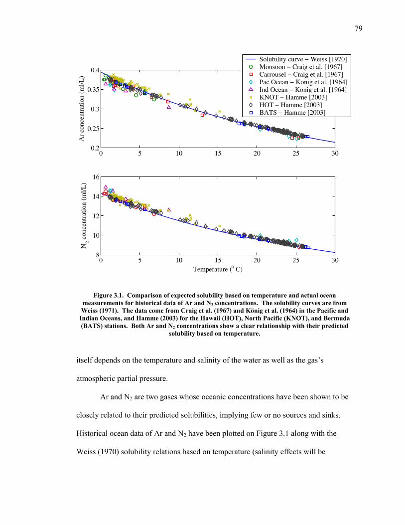
79
Ar
conc
entr
atio
n (m
l/L)
0 5 10 15 20 25 300.2
0.25
0.3
0.35
0.4
Temperature (o C)
N2 c
once
ntra
tion
(ml/L
)
0 5 10 15 20 25 308
10
12
14
16
Solubility curve − Weiss [1970]Monsoon − Craig et al. [1967]Carrousel − Craig et al. [1967]Pac Ocean − Konig et al. [1964]Ind Ocean − Konig et al. [1964]KNOT − Hamme [2003]HOT − Hamme [2003]BATS − Hamme [2003]
Figure 3.1. Comparison of expected solubility based on temperature and actual ocean
measurements for historical data of Ar and N2 concentrations. The solubility curves are from Weiss (1971). The data come from Craig et al. (1967) and König et al. (1964) in the Pacific and
Indian Oceans, and Hamme (2003) for the Hawaii (HOT), North Pacific (KNOT), and Bermuda (BATS) stations. Both Ar and N2 concentrations show a clear relationship with their predicted
solubility based on temperature.
itself depends on the temperature and salinity of the water as well as the gas’s
atmospheric partial pressure.
Ar and N2 are two gases whose oceanic concentrations have been shown to be
closely related to their predicted solubilities, implying few or no sources and sinks.
Historical ocean data of Ar and N2 have been plotted on Figure 3.1 along with the
Weiss (1970) solubility relations based on temperature (salinity effects will be
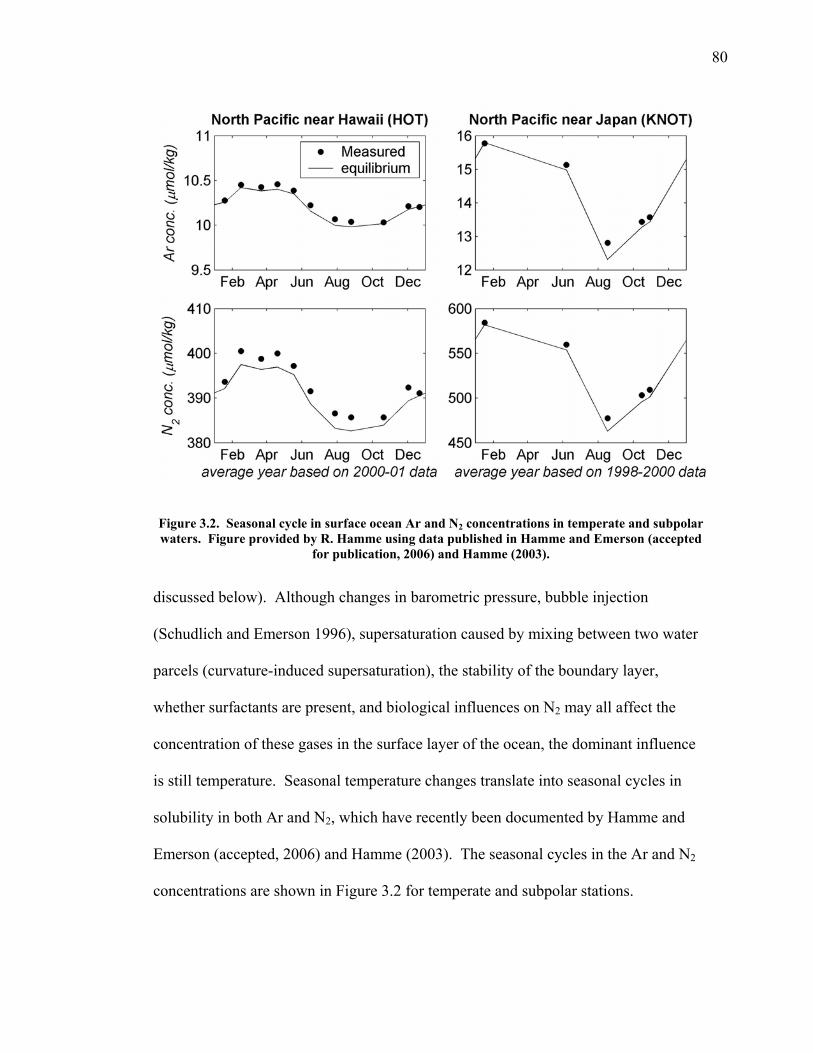
80
Figure 3.2. Seasonal cycle in surface ocean Ar and N2 concentrations in temperate and subpolar waters. Figure provided by R. Hamme using data published in Hamme and Emerson (accepted
for publication, 2006) and Hamme (2003).
discussed below). Although changes in barometric pressure, bubble injection
(Schudlich and Emerson 1996), supersaturation caused by mixing between two water
parcels (curvature-induced supersaturation), the stability of the boundary layer,
whether surfactants are present, and biological influences on N2 may all affect the
concentration of these gases in the surface layer of the ocean, the dominant influence
is still temperature. Seasonal temperature changes translate into seasonal cycles in
solubility in both Ar and N2, which have recently been documented by Hamme and
Emerson (accepted, 2006) and Hamme (2003). The seasonal cycles in the Ar and N2
concentrations are shown in Figure 3.2 for temperate and subpolar stations.
81
As mentioned above, solubility depends on salinity as well as temperature. For
a range of salinity values from 30 to 36 psu, the solubility of Ar and N2 varies by
about 3-4%. Especially in high-latitude areas, however, the solubility may vary more
significantly on seasonal time scales due to changes in freshwater influx and ice
formation and melting. Such seasonal cycles could serve either to amplify or reduce
the effect of air-sea heat flux on the Ar and N2 gas fluxes. Near-surface temperature
and salinity data from the Gulf of Alaska (Okkonen et al. 2005) show clear seasonal
cycles in both variables, ranging between 4-15oC and 18-32 psu. Such seasonal cycles
in salinity could result in changes of up to 10% from the expected amplitude of the
seasonal cycle in solubility of Ar and N2 based solely on temperature changes. Near-
surface float data in the Labrador Sea (A. Koetzinger, pers. comm.) show much
smaller cycles in salinity in near-surface waters, potentially leading to errors of less
than 1% in estimated seasonal cycles of solubility based solely on temperature.
Although it is possible that some regions have large enough cycles in salinity to cause
significant changes in gas solubility, I assume a constant salinity on seasonal time
scales for the following analysis.
For a gas with no major sources and sinks, assuming that it equilibrates rapidly
with the atmosphere, it is possible to estimate air-sea gas flux through the difference in
solubility Sol at the initial and final temperatures, T1 and T2:
( ) ( )( ) .21pc
QT
SolTVT
SolVTSolTSolFluxρΔ
⎟⎠⎞
⎜⎝⎛
∂∂
≈Δ⎟⎠⎞
⎜⎝⎛
∂∂
≈−= (3.1)
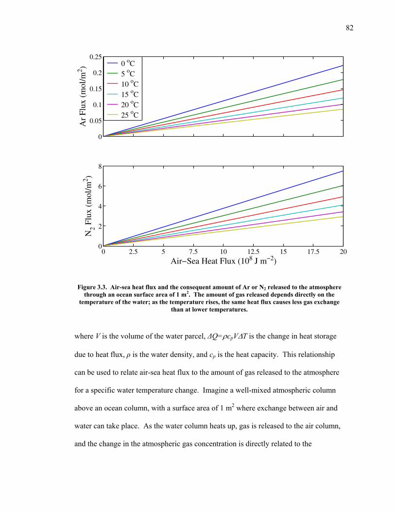
82
Ar
Flux
(m
ol/m
2 )
0
0.05
0.1
0.15
0.2
0.250 oC5 oC10 oC15 oC20 oC25 oC
Air−Sea Heat Flux (108 J m−2)
N2 F
lux
(mol
/m2 )
0 2.5 5 7.5 10 12.5 15 17.5 200
2
4
6
8
Figure 3.3. Air-sea heat flux and the consequent amount of Ar or N2 released to the atmosphere
through an ocean surface area of 1 m2. The amount of gas released depends directly on the temperature of the water; as the temperature rises, the same heat flux causes less gas exchange
than at lower temperatures.
where V is the volume of the water parcel, ΔQ=ρcpVΔT is the change in heat storage
due to heat flux, ρ is the water density, and cp is the heat capacity. This relationship
can be used to relate air-sea heat flux to the amount of gas released to the atmosphere
for a specific water temperature change. Imagine a well-mixed atmospheric column
above an ocean column, with a surface area of 1 m2 where exchange between air and
water can take place. As the water column heats up, gas is released to the air column,
and the change in the atmospheric gas concentration is directly related to the
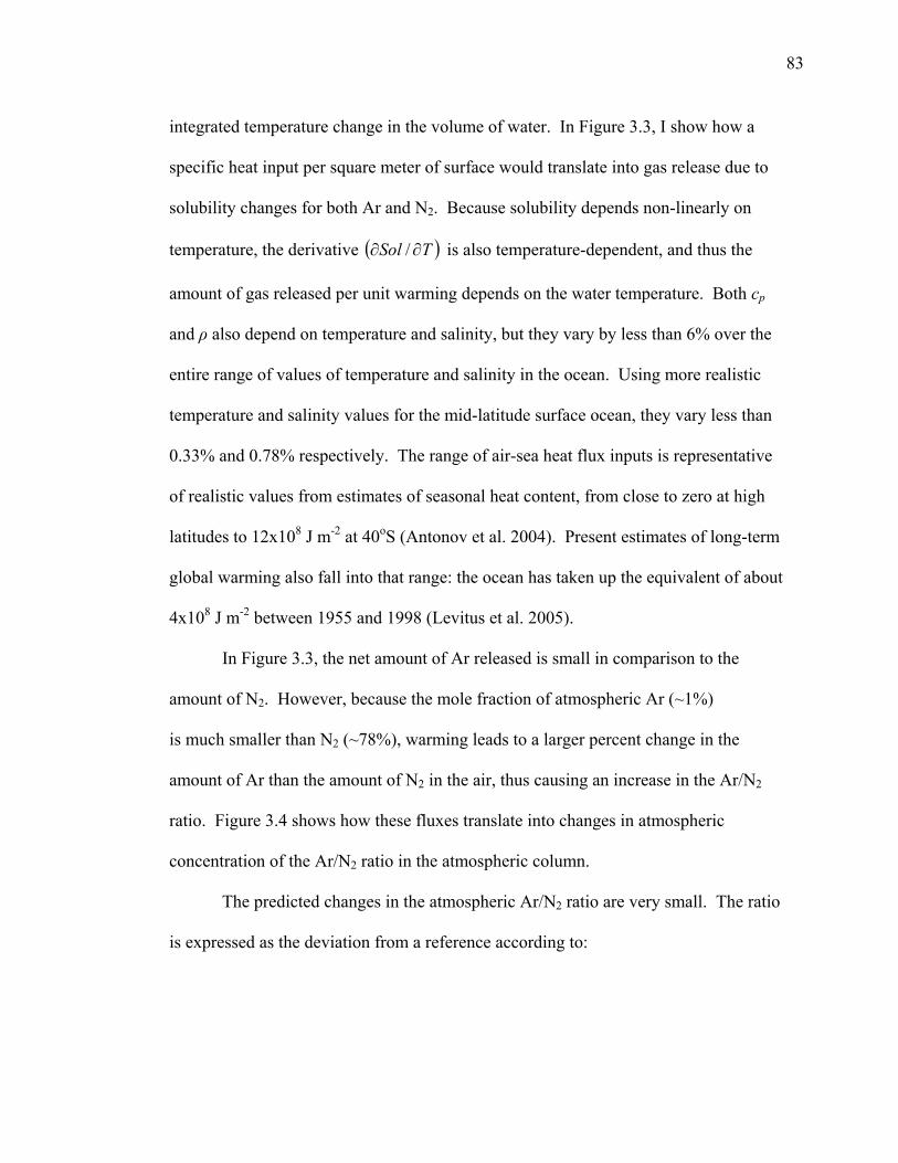
83
integrated temperature change in the volume of water. In Figure 3.3, I show how a
specific heat input per square meter of surface would translate into gas release due to
solubility changes for both Ar and N2. Because solubility depends non-linearly on
temperature, the derivative ( )TSol ∂∂ / is also temperature-dependent, and thus the
amount of gas released per unit warming depends on the water temperature. Both cp
and ρ also depend on temperature and salinity, but they vary by less than 6% over the
entire range of values of temperature and salinity in the ocean. Using more realistic
temperature and salinity values for the mid-latitude surface ocean, they vary less than
0.33% and 0.78% respectively. The range of air-sea heat flux inputs is representative
of realistic values from estimates of seasonal heat content, from close to zero at high
latitudes to 12x108 J m-2 at 40oS (Antonov et al. 2004). Present estimates of long-term
global warming also fall into that range: the ocean has taken up the equivalent of about
4x10⁸ J m-2 between 1955 and 1998 (Levitus et al. 2005).
In Figure 3.3, the net amount of Ar released is small in comparison to the
amount of N2. However, because the mole fraction of atmospheric Ar (~1%)
is much smaller than N2 (~78%), warming leads to a larger percent change in the
amount of Ar than the amount of N2 in the air, thus causing an increase in the Ar/N2
ratio. Figure 3.4 shows how these fluxes translate into changes in atmospheric
concentration of the Ar/N2 ratio in the atmospheric column.
The predicted changes in the atmospheric Ar/N2 ratio are very small. The ratio
is expressed as the deviation from a reference according to:
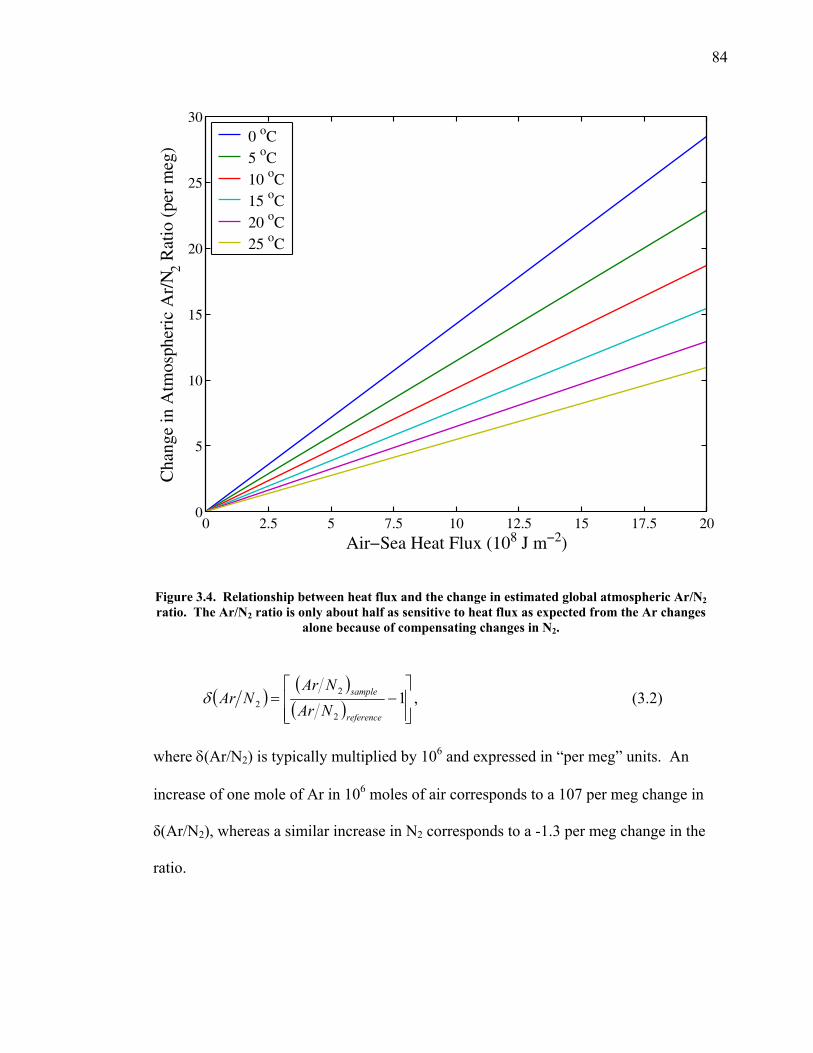
84
Cha
nge
in A
tmos
pher
ic A
r/N
2 Rat
io (
per
meg
)
Air−Sea Heat Flux (108 J m−2)0 2.5 5 7.5 10 12.5 15 17.5 20
0
5
10
15
20
25
300 oC5 oC10 oC15 oC20 oC25 oC
Figure 3.4. Relationship between heat flux and the change in estimated global atmospheric Ar/N2 ratio. The Ar/N2 ratio is only about half as sensitive to heat flux as expected from the Ar changes
alone because of compensating changes in N2.
( )( )
( ) ⎥⎥⎦
⎤
⎢⎢⎣
⎡−= 1
2
22
reference
sample
NArNAr
NArδ , (3.2)
where δ(Ar/N2) is typically multiplied by 106 and expressed in “per meg” units. An
increase of one mole of Ar in 106 moles of air corresponds to a 107 per meg change in
δ(Ar/N2), whereas a similar increase in N2 corresponds to a -1.3 per meg change in the
ratio.
85
Equation 3.1 and the results of Figures 3.3-3.4 assume that atmospheric and
oceanic concentrations of Ar and N2 equilibrate instantaneously and completely. In
reality, it takes time for the ocean to equilibrate with respect to the atmosphere. This
delay is usually modeled as the following:
( )eqCCKFlux −= , (3.3)
which relates the gas flux to the disequilibrium in the surface water. K is called the
piston velocity or transfer velocity, describing how fast gas exchange penetrates
through the laminar layer. Theoretical studies of momentum and mass transfer have
suggested that K should be dependent on the ratio of transfer coefficients for
momentum (the kinematic viscosity υ) and mass (molecular diffusivity D). In
practice, the value of K can vary extensively in different environmental conditions and
for different gases (Liss and Merlivat 1986; Jähne and Hauβecker 1998; Jähne et al.
1987; Jean-Baptiste and Poisson 2000; Wanninkhof 1992).
A two-box model of the oceanic mixed layer and the overlying atmosphere can
be used to illustrate the seasonal changes in atmospheric δ(Ar/N2), allowing for finite
rather than infinite K (Figure 3.5). Changes in the concentration of the ocean box are
directly dependent on the flux to the atmosphere:
( ) ,FAdtdCV −= or ( ) ,FdtdCH −= (3.4)
where V is the volume of the box, F is the flux to the atmosphere, A is the area of the
surface, and H is the depth of the box. The atmosphere and ocean boxes are assumed
to be well-mixed. Combining 3.3 and 3.4 and isolating the change in the equilibrium
concentration yields:
86
Figure 3.5. Diagram of the transient model showing the gas flux between ocean and atmosphere.
( ) ( ) .dt
dCCC
HK
dtCCd eq
eqeq −−−=
− (3.5)
This formulation gives an exchange time constant of H/K. Since the salinity and
pressure effects on solubility at the ocean surface are small, the term dCeq/dt can be
considered as a thermal forcing term, assuming that only changes in the temperature of
the ocean surface drive changes in the equilibrium concentration.
Solubility depends almost linearly on temperature over small temperature
changes. It is thus possible to estimate the equilibrium concentration of a particular
species in water as a linear function of the temperature:
.1CTCeq += α (3.6)
In this two-box model, if we assume that temperature of the ocean box (or mixed
layer) changes in a sinusoidal way over time, then we can also write the equilibrium
concentration as the following:
87
( ) 2sin CtTCeq +−Δ= ϕωα , (3.7)
where α is the derivative of solubility with respect to temperature, ΔT is the amplitude
of the seasonal cycle in temperature, ω = 2π/365 days, φ is a given phase, and C2 is a
constant. The equilibrium value of C therefore changes over a year in the same
sinusoidal way as temperature.
This model is solved by Keeling et al. (1993) to give the following solution:
( )( ),cos ϕωαω−−Δ⎟
⎠⎞
⎜⎝⎛=− lageq ttTf
KHCC (3.8)
where 212
1−
⎟⎟⎠
⎞⎜⎜⎝
⎛⎟⎠⎞
⎜⎝⎛+=
KHf ϖ and .tan1 1 ⎟
⎠⎞
⎜⎝⎛
⎟⎠⎞
⎜⎝⎛= −
KHtlag
ϖϖ
The parameter f basically describes how efficiently the gas equilibrates with the
atmosphere, whereas tlag describes the delay between forcing and response. The time-
integrated air-sea gas flux and the related heat flux can be written as the following,
integrated from zero to a given time:
( )( ),sin∫ −−Δ= ϕωα lagttTHfFdt and (3.9)
.THcQ p Δ=Δ ρ (3.10)
Using these equations to calculate the flux of Ar and N2, I can then calculate
δ(Ar/N2). For small changes, δ(Ar/N2) can be approximated by the difference in the
relative change of Ar and N2 in the atmosphere:
( ) ( ) ( ) 6
2
22 10⋅⎟⎟
⎠
⎞⎜⎜⎝
⎛Χ
−Χ
=N
atmN
Ar
atmAr MFMFNArδ , (3.11)
88
where FAr and FN2 are the fluxes of Ar and N2 in moles per m2 of exchange surface,
Matm is the number of moles of air in the atmospheric box per m2 of exchange surface,
and ΧAr and ΧN2 are the average atmospheric mole fraction of Ar and N2 respectively.
The amount of moles in the atmospheric column is calculated from the total number of
moles in the atmosphere (1.8x10²⁰) divided by the surface area of the earth. Eqation
(3.11) can also be written in terms of the heat flux:
( ) 6
2
222 10⋅⎟⎟
⎠
⎞⎜⎜⎝
⎛Χ
−Χ
Δ=
N
NN
Ar
ArAr
patm
ffcMQNAr
ααρ
δ . (3.12)
For this model, I assume that all the air in this column mixes instantaneously. This is
far from the actuality, as air is transported both horizontally as well as vertically, and
vertical mixing can have a time constant of months to years. Decreasing the estimated
size of this box would increase the expected change in δ(Ar/N2).
I calculate the seasonal cycle in δ(Ar/N2) due to air-sea heat flux under
idealized conditions. The following results assume inputs of approximate values for a
temperate ocean mixed layer, with a box depth of 80 m and a seasonal temperature
cycle of ± 2oC in the mixed layer around a mean temperature of 15oC. This
temperature range is consistent with values of average seasonal heat storage estimated
for the Atlantic basin by the TOPEX data. I adopt K values of 3.47 m day-1 for Ar and
3.64 m day-1 for N2, following Keeling et al. (1993) and taking into account small
changes in molecular diffusion rates between the two species. Figure 3.6 gives the
seasonal cycle of atmospheric δ(Ar/N2), showing the contributions of both Ar and N2.
The annual flux cycle for the individual gases are also plotted against heat flux (see
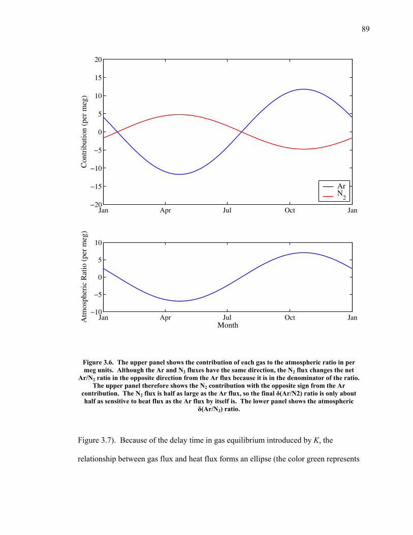
89
Con
trib
utio
n (p
er m
eg)
Jan Apr Jul Oct Jan−20
−15
−10
−5
0
5
10
15
20
Month
Atm
osph
eric
Rat
io (
per
meg
)
Jan Apr Jul Oct Jan−10
−5
0
5
10
ArN
2
Figure 3.6. The upper panel shows the contribution of each gas to the atmospheric ratio in per meg units. Although the Ar and N2 fluxes have the same direction, the N2 flux changes the net
Ar/N2 ratio in the opposite direction from the Ar flux because it is in the denominator of the ratio. The upper panel therefore shows the N2 contribution with the opposite sign from the Ar
contribution. The N2 flux is half as large as the Ar flux, so the final δ(Ar/N2) ratio is only about half as sensitive to heat flux as the Ar flux by itself is. The lower panel shows the atmospheric
δ(Ar/N2) ratio.
Figure 3.7). Because of the delay time in gas equilibrium introduced by K, the
relationship between gas flux and heat flux forms an ellipse (the color green represents
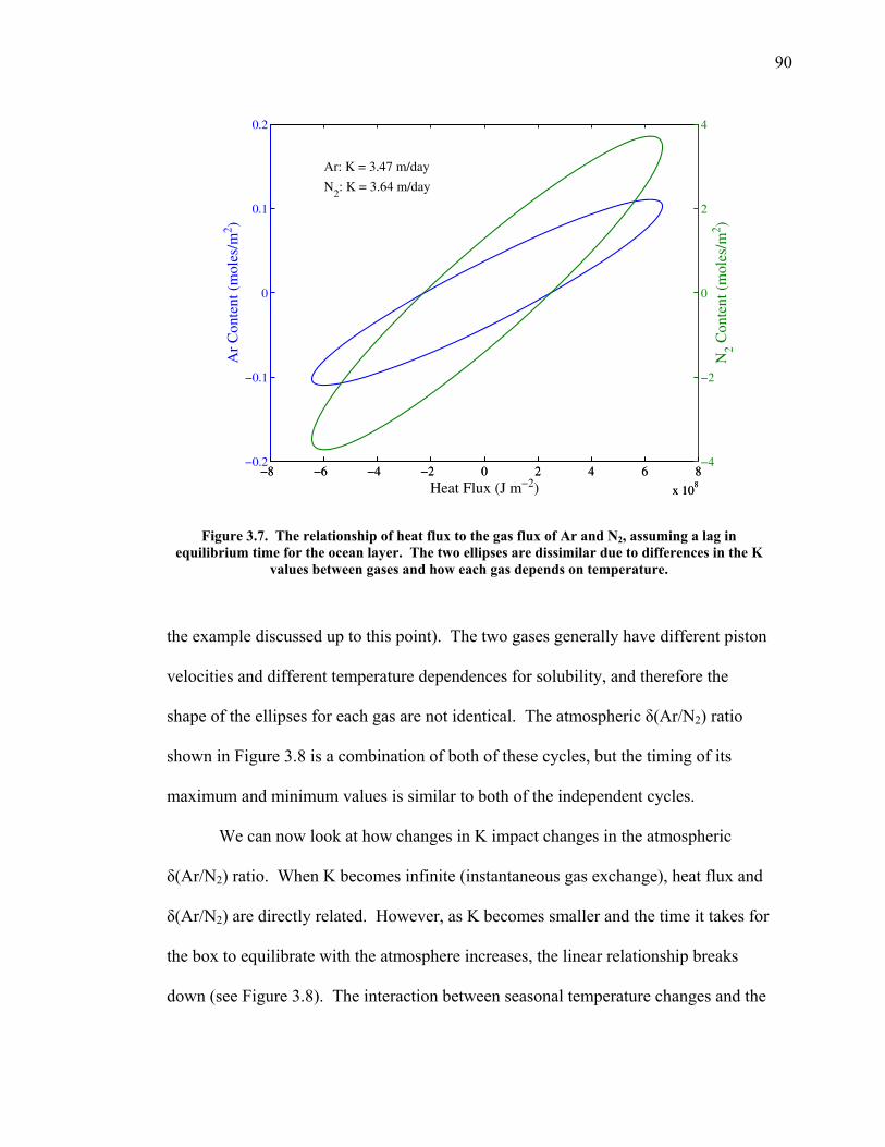
90
Ar: K = 3.47 m/day
N2: K = 3.64 m/day
Heat Flux (J m−2)
Ar
Con
tent
(m
oles
/m2 )
−8 −6 −4 −2 0 2 4 6 8
x 108
−0.2
−0.1
0
0.1
0.2
N2 C
onte
nt (
mol
es/m
2 )
−8 −6 −4 −2 0 2 4 6 8
x 108
−4
−2
0
2
4
Figure 3.7. The relationship of heat flux to the gas flux of Ar and N2, assuming a lag in equilibrium time for the ocean layer. The two ellipses are dissimilar due to differences in the K
values between gases and how each gas depends on temperature.
the example discussed up to this point). The two gases generally have different piston
velocities and different temperature dependences for solubility, and therefore the
shape of the ellipses for each gas are not identical. The atmospheric δ(Ar/N2) ratio
shown in Figure 3.8 is a combination of both of these cycles, but the timing of its
maximum and minimum values is similar to both of the independent cycles.
We can now look at how changes in K impact changes in the atmospheric
δ(Ar/N2) ratio. When K becomes infinite (instantaneous gas exchange), heat flux and
δ(Ar/N2) are directly related. However, as K becomes smaller and the time it takes for
the box to equilibrate with the atmosphere increases, the linear relationship breaks
down (see Figure 3.8). The interaction between seasonal temperature changes and the
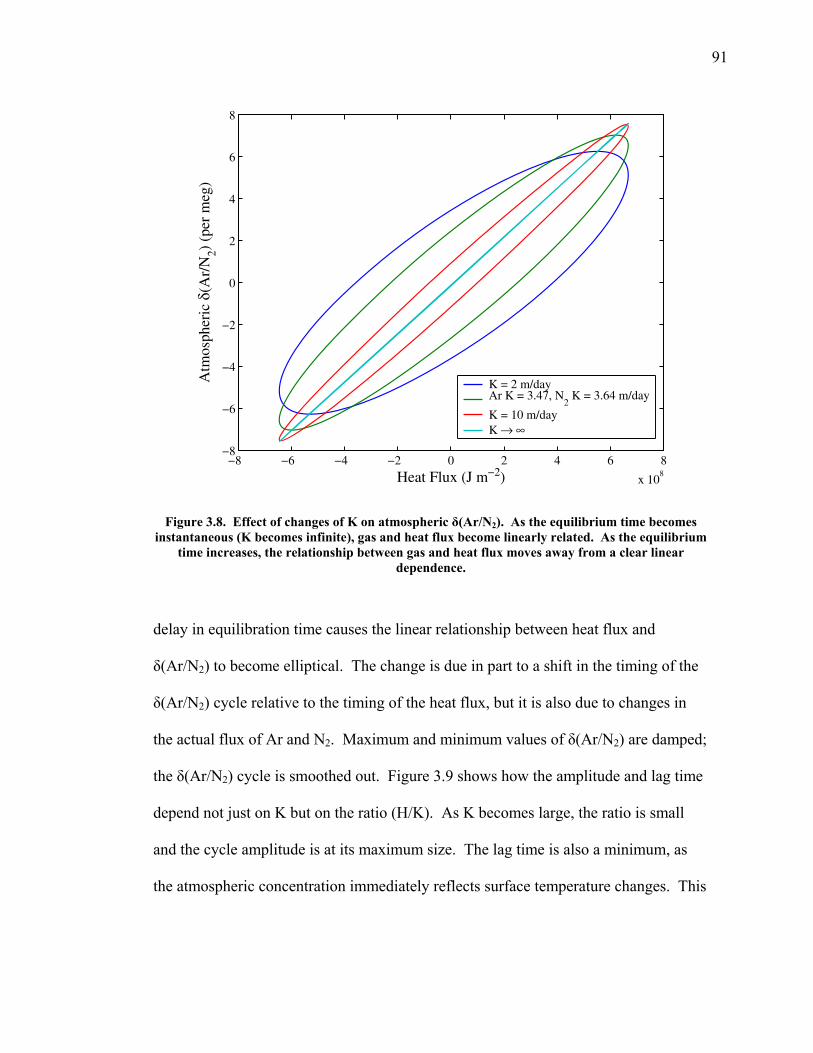
91
Heat Flux (J m−2)
Atm
osph
eric
δ(A
r/N
2) (p
er m
eg)
−8 −6 −4 −2 0 2 4 6 8
x 108
−8
−6
−4
−2
0
2
4
6
8
K = 2 m/dayAr K = 3.47, N
2 K = 3.64 m/day
K = 10 m/dayK → ∞
Figure 3.8. Effect of changes of K on atmospheric δ(Ar/N2). As the equilibrium time becomes instantaneous (K becomes infinite), gas and heat flux become linearly related. As the equilibrium
time increases, the relationship between gas and heat flux moves away from a clear linear dependence.
delay in equilibration time causes the linear relationship between heat flux and
δ(Ar/N2) to become elliptical. The change is due in part to a shift in the timing of the
δ(Ar/N2) cycle relative to the timing of the heat flux, but it is also due to changes in
the actual flux of Ar and N2. Maximum and minimum values of δ(Ar/N2) are damped;
the δ(Ar/N2) cycle is smoothed out. Figure 3.9 shows how the amplitude and lag time
depend not just on K but on the ratio (H/K). As K becomes large, the ratio is small
and the cycle amplitude is at its maximum size. The lag time is also a minimum, as
the atmospheric concentration immediately reflects surface temperature changes. This
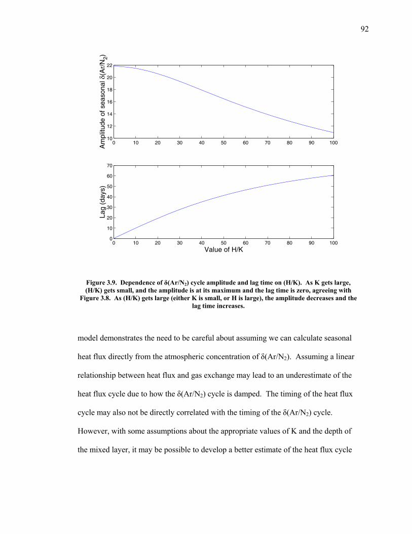
92
0 10 20 30 40 50 60 70 80 90 10010
12
14
16
18
20
22
Am
plitu
de o
f sea
sona
l δ(A
r/N
2)
0 10 20 30 40 50 60 70 80 90 1000
10
20
30
40
50
60
70
Lag
(day
s)
Value of H/K
Figure 3.9. Dependence of δ(Ar/N2) cycle amplitude and lag time on (H/K). As K gets large, (H/K) gets small, and the amplitude is at its maximum and the lag time is zero, agreeing with
Figure 3.8. As (H/K) gets large (either K is small, or H is large), the amplitude decreases and the lag time increases.
model demonstrates the need to be careful about assuming we can calculate seasonal
heat flux directly from the atmospheric concentration of δ(Ar/N2). Assuming a linear
relationship between heat flux and gas exchange may lead to an underestimate of the
heat flux cycle due to how the δ(Ar/N2) cycle is damped. The timing of the heat flux
cycle may also not be directly correlated with the timing of the δ(Ar/N2) cycle.
However, with some assumptions about the appropriate values of K and the depth of
the mixed layer, it may be possible to develop a better estimate of the heat flux cycle
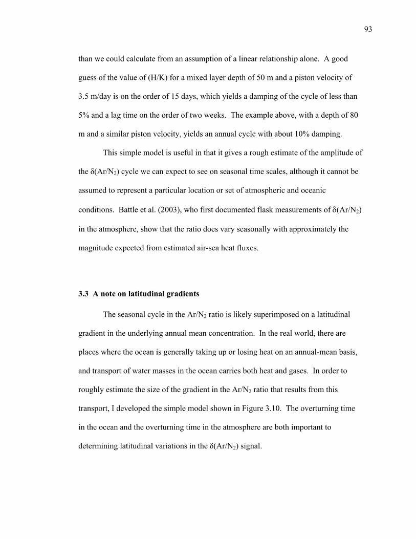
93
than we could calculate from an assumption of a linear relationship alone. A good
guess of the value of (H/K) for a mixed layer depth of 50 m and a piston velocity of
3.5 m/day is on the order of 15 days, which yields a damping of the cycle of less than
5% and a lag time on the order of two weeks. The example above, with a depth of 80
m and a similar piston velocity, yields an annual cycle with about 10% damping.
This simple model is useful in that it gives a rough estimate of the amplitude of
the δ(Ar/N2) cycle we can expect to see on seasonal time scales, although it cannot be
assumed to represent a particular location or set of atmospheric and oceanic
conditions. Battle et al. (2003), who first documented flask measurements of δ(Ar/N2)
in the atmosphere, show that the ratio does vary seasonally with approximately the
magnitude expected from estimated air-sea heat fluxes.
3.3 A note on latitudinal gradients
The seasonal cycle in the Ar/N2 ratio is likely superimposed on a latitudinal
gradient in the underlying annual mean concentration. In the real world, there are
places where the ocean is generally taking up or losing heat on an annual-mean basis,
and transport of water masses in the ocean carries both heat and gases. In order to
roughly estimate the size of the gradient in the Ar/N2 ratio that results from this
transport, I developed the simple model shown in Figure 3.10. The overturning time
in the ocean and the overturning time in the atmosphere are both important to
determining latitudinal variations in the δ(Ar/N2) signal.
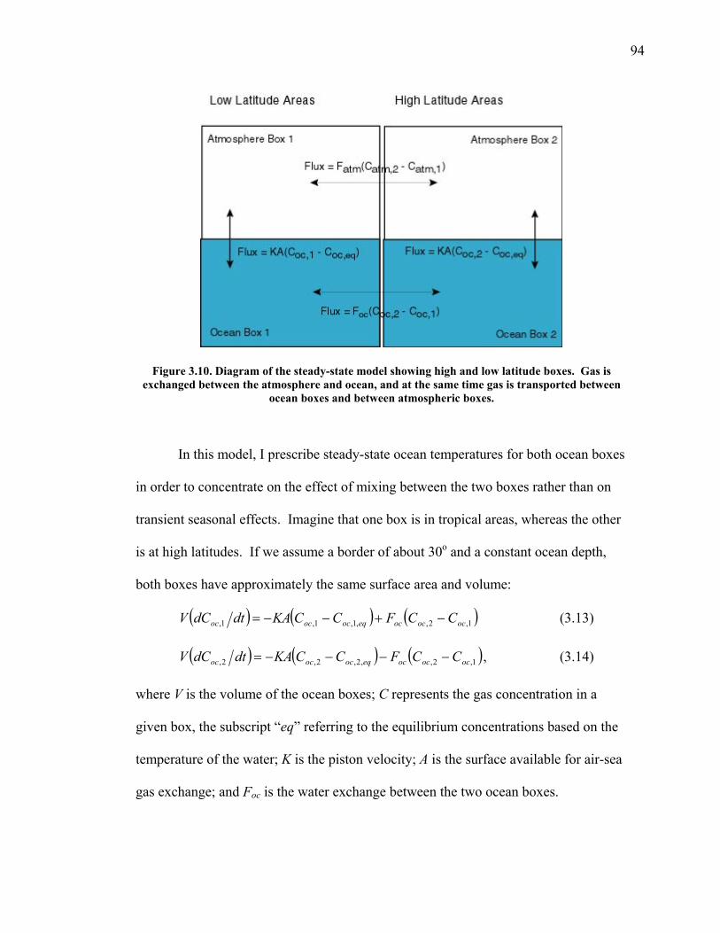
94
Figure 3.10. Diagram of the steady-state model showing high and low latitude boxes. Gas is exchanged between the atmosphere and ocean, and at the same time gas is transported between
ocean boxes and between atmospheric boxes.
In this model, I prescribe steady-state ocean temperatures for both ocean boxes
in order to concentrate on the effect of mixing between the two boxes rather than on
transient seasonal effects. Imagine that one box is in tropical areas, whereas the other
is at high latitudes. If we assume a border of about 30o and a constant ocean depth,
both boxes have approximately the same surface area and volume:
( ) ( ) ( )1,2,,1,1,1, ocococeqocococ CCFCCKAdtdCV −+−−= (3.13)
( ) ( ) ( )1,2,,2,2,2, ocococeqocococ CCFCCKAdtdCV −−−−= , (3.14)
where V is the volume of the ocean boxes; C represents the gas concentration in a
given box, the subscript “eq” referring to the equilibrium concentrations based on the
temperature of the water; K is the piston velocity; A is the surface available for air-sea
gas exchange; and Foc is the water exchange between the two ocean boxes.
95
In the previous model, the equilibrium concentrations in the ocean have a
seasonal cycle dependent on the temperature of the water. The air-sea gas fluxes are
small in comparison to the amount of gas stored in the ocean, and so the atmospheric
Ar/N2 ratio changes in response to the ocean equilibrium concentration. As stated
above, however, the temperature of the water and the equilibrium concentrations in
each box in this model are fixed in order to focus on the gradient due to ocean heat
transport. The atmospheric boxes are therefore decoupled from the oceanic boxes.
The solutions for the gas concentrations in the ocean boxes are the following:
γγ+
⋅+=
1,1,,
1,eqocavgoc
oc
CCC , (3.15)
γγ+
⋅+=
1,2,,
2,eqocavgoc
oc
CCC , (3.16)
where ( )( ) eq
mixoc
oc KHFV
FKA
ττ
γ222
=== .
V/Foc represents the exchange time τmix of water masses between the two boxes, or
how quickly the water in one box is replaced, whereas H/K, seen also in the first
model, represents the gas equilibrium time τeq with respect to air-sea exchange.
The atmospheric concentrations of Ar and N2 are forced by the fluxes in and
out of the ocean box. However, exchange between the atmospheric boxes also
influences the final, equilibrium concentration. The changes in the atmospheric box
concentrations are described by the following:
( ) ( ) ( )1,2,,1,1,1, atmatmatmeqococatm CCFCCKAdtdCV −+−= (3.17)
( ) ( ) ( )1,2,,2,2,2, atmatmatmeqococatm CCFCCKAdtdCV −−−= , (3.18)
96
where Catm,1 and Catm,2 are the respective atmospheric concentrations above the ocean
boxes, and Fatm is the air exchange between atmospheric boxes. For the rest of the
discussion, I assume that Catm,avg = 0 and look only at the difference in the
concentrations between the two atmospheric boxes. In this case, the solutions are as
follows:
( )eqoceqocatm
ocavgatmatm CC
FF
CC ,2,,1,,1, 12−⎟⎟
⎠
⎞⎜⎜⎝
⎛+⎟⎟
⎠
⎞⎜⎜⎝
⎛−=
γγ , and (3.19)
( )eqoceqocatm
ocavgatmatm CC
FF
CC ,2,,1,,2, 12−⎟⎟
⎠
⎞⎜⎜⎝
⎛+⎟⎟
⎠
⎞⎜⎜⎝
⎛+=
γγ , (3.20)
For subsequent analysis, I assume that K is the same for both Ar and N2. I fix the
ocean transport at 50 Sv and the box temperatures at 13oC for the low latitudes and
3.75oC for the high latitudes, consistent with estimates of a 2 PW heat flux carried
both by eddy transport and thermohaline circulation in the Northern Hemisphere
(Talley 1999). The atmospheric transport is assigned to be 8.7x10¹² moles of air per
second, consistent with an intrahemispheric overturning time of two months.
Figure 3.11 shows the value of atmospheric δ(Ar/N2) relative to γ. γ describes
how the gas equilibrium time relates to the exchange time of water masses between
the two ocean boxes. As γ becomes small, the concentrations in both ocean and
atmosphere boxes approach each other and the gas flux drops. In contrast, as γ
becomes large, the concentration of each box approaches its equilibrium
concentration. In practice, it is difficult to come up with a good measure of γ. With
an 80 m mixed layer, Ar and N2 have an equilibration time constant of about a month.
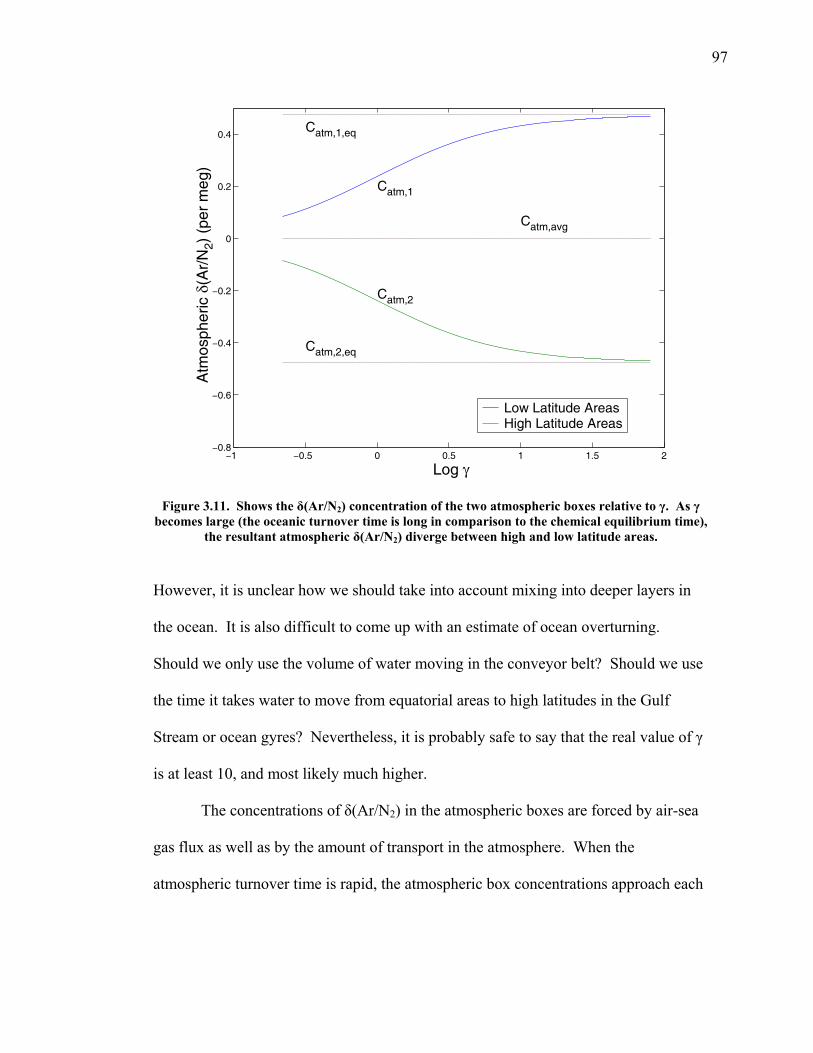
97
−1 −0.5 0 0.5 1 1.5 2−0.8
−0.6
−0.4
−0.2
0
0.2
0.4
Log γ
Atm
osph
eric
δ(A
r/N
2) (
per
meg
)
Catm,2,eq
Catm,1,eq
Catm,2
Catm,1
Catm,avg
Low Latitude AreasHigh Latitude Areas
Figure 3.11. Shows the δ(Ar/N2) concentration of the two atmospheric boxes relative to γ. As γ becomes large (the oceanic turnover time is long in comparison to the chemical equilibrium time),
the resultant atmospheric δ(Ar/N2) diverge between high and low latitude areas.
However, it is unclear how we should take into account mixing into deeper layers in
the ocean. It is also difficult to come up with an estimate of ocean overturning.
Should we only use the volume of water moving in the conveyor belt? Should we use
the time it takes water to move from equatorial areas to high latitudes in the Gulf
Stream or ocean gyres? Nevertheless, it is probably safe to say that the real value of γ
is at least 10, and most likely much higher.
The concentrations of δ(Ar/N2) in the atmospheric boxes are forced by air-sea
gas flux as well as by the amount of transport in the atmosphere. When the
atmospheric turnover time is rapid, the atmospheric box concentrations approach each
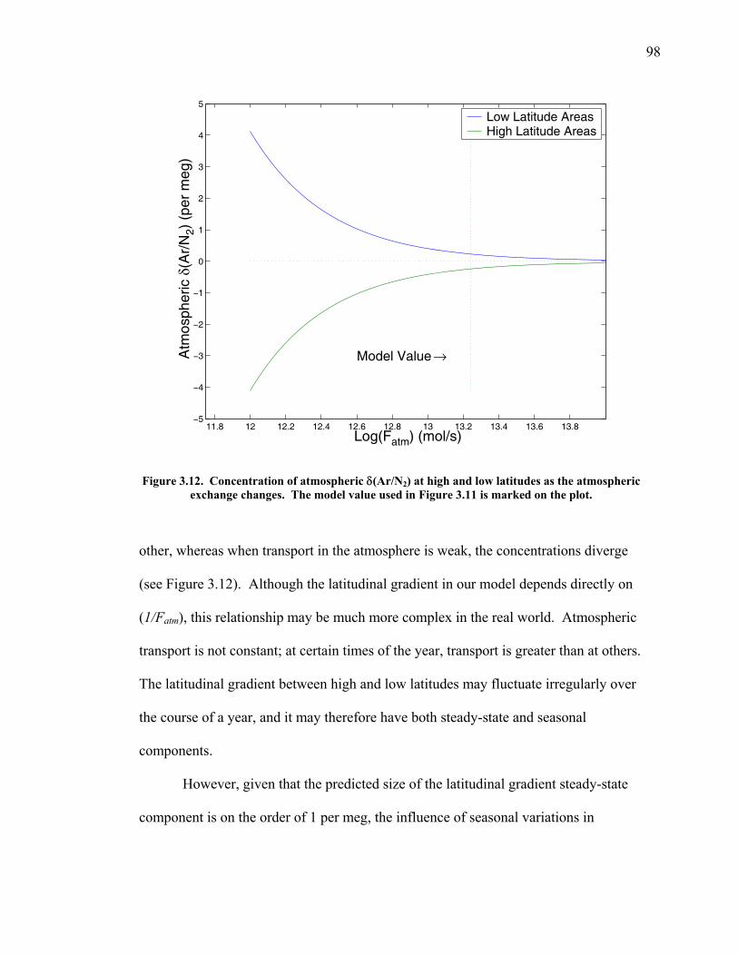
98
11.8 12 12.2 12.4 12.6 12.8 13 13.2 13.4 13.6 13.8−5
−4
−3
−2
−1
0
1
2
3
4
5
Log(Fatm) (mol/s)
Atm
osph
eric
δ(A
r/N
2) (
per
meg
)
Model Value →
Low Latitude AreasHigh Latitude Areas
Figure 3.12. Concentration of atmospheric δ(Ar/N2) at high and low latitudes as the atmospheric exchange changes. The model value used in Figure 3.11 is marked on the plot.
other, whereas when transport in the atmosphere is weak, the concentrations diverge
(see Figure 3.12). Although the latitudinal gradient in our model depends directly on
(1/Fatm), this relationship may be much more complex in the real world. Atmospheric
transport is not constant; at certain times of the year, transport is greater than at others.
The latitudinal gradient between high and low latitudes may fluctuate irregularly over
the course of a year, and it may therefore have both steady-state and seasonal
components.
However, given that the predicted size of the latitudinal gradient steady-state
component is on the order of 1 per meg, the influence of seasonal variations in
99
transport is likely to be even smaller. My estimate of the latitudinal gradient is most
likely low; in my model, I assumed both instantaneous horizontal and vertical mixing.
In reality, surface concentrations are likely to be higher due to slow mixing times, and
we may see a larger gradient in annual mean concentrations, particularly at the
surface.
The latitudinal gradient in atmospheric δ(Ar/N2) is likely to be small in
comparison to the seasonal cycle in δ(Ar/N2) at any given station. A higher level of
measurement precision may be required to determine and compare the annual mean
concentration at stations along a latitudinal gradient.
3.4 Global maps of the expected seasonal cycle in surface δ(Ar/N2)
The previous models provide rough estimates for the changes in the Ar/N2
ratio in an atmospheric column in response to ocean warming and cooling and for a
latitudinal gradient. However, they cannot provide realistic predictions of the ratio at
a given location. Here I use atmospheric transport models to develop more realistic
estimates of the seasonal variations in the Ar/N2 ratio.
In order to develop maps of the seasonal cycle (ignoring any mean values), I
used the predictions of atmospheric N2 concentrations from the models in Chapter 2.
The N2 fluxes were calculated from the same principle (Equation 3.1) as that used in
the conceptual box model described in section 3.2. Because the effect of the air-sea
flux of N2 in atmospheric per meg units is very similar to that of Ar, I multiply the
change in the atmospheric N2 concentration by a constant scale factor of 1.48 to
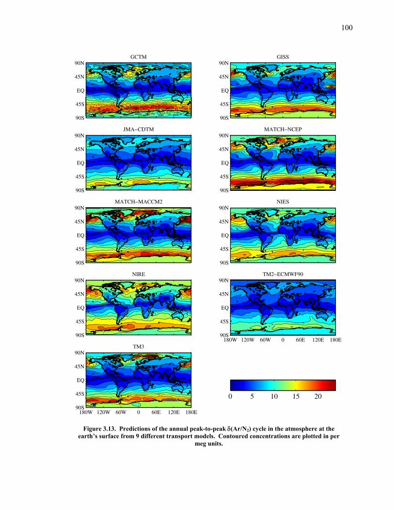
100
GCTM
90S
45S
EQ
45N
90NGISS
90S
45S
EQ
45N
90N
JMA−CDTM
90S
45S
EQ
45N
90NMATCH−NCEP
90S
45S
EQ
45N
90N
MATCH−MACCM2
90S
45S
EQ
45N
90NNIES
90S
45S
EQ
45N
90N
NIRE
90S
45S
EQ
45N
90NTM2−ECMWF90
180W 120W 60W 0 60E 120E 180E90S
45S
EQ
45N
90N
TM3
180W 120W 60W 0 60E 120E 180E90S
45S
EQ
45N
90N
0 5 10 15 20
Figure 3.13. Predictions of the annual peak-to-peak δ(Ar/N2) cycle in the atmosphere at the earth’s surface from 9 different transport models. Contoured concentrations are plotted in per
meg units.
101
calculate the expected seasonal concentration of δ(Ar/N2). This scale factor is taken
from the ratio of changes in atmospheric Ar to N2 in the two-box model described
earlier. Although small differences in the relationships between the solubility of Ar
and N2 with temperature should cause this factor to change slightly, it is not enough to
be significant. The seasonal peak-to-peak amplitude predictions are shown in the
model maps in Figure 3.13. The largest annual cycles correspond well, not
surprisingly, with the areas with the largest seasonal air-sea heat flux, in the northern
and southern latitudes of 45-60o, and are smallest in equatorial areas.
Most importantly, these maps give an idea of how well we need to be able to
measure the atmospheric δ(Ar/N2) ratio in order to contribute useful information on
air-sea heat fluxes. The predictions suggest that we need to be able to accurately
measure a seasonal cycle of 12-17 per meg at mid- to high-latitude stations where air-
sea heat flux is most important, and to be able to measure an even smaller seasonal
cycle to get useful information at lower latitudes. Because the models also use winds
from different years, the variation between the models may give us an idea of the size
of interannual variability in the δ(Ar/N2) cycle, possibly ranging from 10-25 per meg
in peak-to-peak amplitude at some places.
3.5 Conclusions
The present state of ocean measurements of air-sea heat flux and ocean heat
content suggests the need for independent methods for measuring ocean heat uptake
102
on seasonal and interannual time scales. Because of the close correlation in air-sea
heat flux and atmospheric δ(Ar/N2), regular measurements may serve to independently
estimate air-sea heat flux and provide information on its temporal variability.
Atmospheric tracer transport models suggest how well we need to be able to measure
the annual δ(Ar/N2) cycle in order to gain new information: the goal needs to be
measurements good enough to identify an annual peak-to-peak cycle of 12-17 per meg
in mid-latitude areas. Better measurements may be necessary to look more closely at
interannual variability in air-sea heat flux.
103
3.6 Bibliography
Antonov, J. I., S. Levitus, and T. P. Boyer. 2004. Climatological annual cycle of ocean heat content. Geophys. Res. Lett. 31 (doi: 10.1029/2003GLO18851).
Battle, M., M. Bender, M. B. Hendricks, D. T. Ho, R. Mika, G. McKinley, S.-M. Fan,
T. Blaine, and R. F. Keeling. 2003. Measurements and models of the atmospheric Ar/N2 ratio. Geophys. Res. Lett. 30 (doi: 10.1029/2003GL017411).
Barnett, T. P., D. W. Pierce, K. M. AchutaRao, P. J. Gleckler, B. D. Santer, J. M.
Gregory, and W. M. Washington. 2005. Penentration of human-induced warming into the world’s oceans. Science 309: 284-287.
Barnett, T. P., D. W. Pierce, and R. Schnur. 2001. Detection of anthropogenic
climate change in the world’s oceans. Science 292: 270-274. Chambers, D. P., B. D. Tapley, and R. H. Stewart. 1997. Long-period ocean heat
storage rates and basin-scale heat fluxes from TOPEX. J. Geophys. Res. 102: 10,525-10,533.
Craig, H., R. F. Weiss, and W. B. Clarke. 1967. Dissolved gases in the equatorial and
south Pacific Ocean. J. Geophys. Res. 72: 6165-6181. Ganachaud, A. and C. Wunsch. 2000. Improved estimates of global ocean
circulation, heat transport and mixing from hydrographic data. Nature 408: 453-457.
Gille, S. T. 2002. Warming of the Southern Ocean since the 1950s. Science 295:
1275-1277. Glueckauf, E. 1951. The composition of atmospheric air. Compendium of
Meteorology. Am. Met. Soc. Boston, 3-11. Hamme, R. C. 2003. Applications of neon, nitrogen, argon and oxygen to chemical,
physical, and biological cycles in the ocean. Ph.D. thesis: University of Washington.
Hamme, R. C. and S. R. Emerson. 2006. Constraining bubble dynamics and mixing
on dissolved gases: Implications for productivity measurements by oxygen mass balance. J. Mar. Res.: in press.
Houghton, J. T., Y. Ding, D. J. Griggs, M. Noguer, P. J. van der Linden, X. Dai, K.
Maskell, and C. A. Johnson (eds). 2001. Climate Change 2001: The
104
Scientific Basis (Contribution of Working Group I to the Third Assessment Report of the Intergovernmental Panel on Climate Change). Cambridge University Press: Cambridge, U.K., and New York, U.S.A.
Hsiung, J., R. E. Newell, and T. Houghtby. 1989. The annual cycle of oceanic heat
storage and oceanic meridional heat transport. Q. J. Roy. Meteor. Soc. 115: 1-28.
Jähne, B. and H. Hauβecker. 1998. Air-water gas exchange. Ann. Rev. Fluid Mech.
30: 443-468
Jähne, B., G. Heinz, and W. Dietrich. 1987. Measurement of the diffusion coefficients of sparingly soluble gases in water. J. Geophys. Res. 92: 10,767-10,776.
Jean-Baptiste, P. and A. Poisson. 2000. Gas transfer experiment on a lake (Kerguelen
Islands) using 3He and SF6. J. Geophys. Res. 105: 1177-1186. Keeling, R. F., R. P. Najjar, M. L. Bender, P. P. Tans. 1993. What atmospheric
oxygen measurements can tell us about the global carbon cycle. Glob. Biogeochem. Cycles 7: 37-67.
König, H., H. Wänke, G. S. Bien, N. W. Rakestraw, and H. E. Suess. 1964. Helium,
neon, and argon in the oceans. Deep-Sea Res. 11 : 243-247. Levitus, S. 1987. Rate of change of heat storage of the world ocean. J. Phys.
Oceanogr. 17 : 518-528. Levitus, S., J. Antonov, and T. Boyer. 2005. Warming of the world ocean, 1955-
2003. Geophys. Res. Lett. 32, L02604 (doi: 10.1029/2004GL021592). Levitus, S., J. I. Antonov, T. P. Boyer, and C. Stephens. 2000. Warming of the world
ocean. Science 287: 2225-2228. Levitus, S., J. I. Antonov, J. Wang, T. L. Delworth, K. W. Dixon, and A. J. Broccoli.
2001. Anthropogenic warming of the earth’s climate system. Science 292: 267-270.
Liss, P. S. and L. Merlivat. 1986. Air-sea gas exchange rates: introduction and
synthesis. Pages 113-127 in: P. Buat-Ménard (ed.). The Role of Air-Sea Exchange in Geochemical Cycling. D. Reidel Publishing Co.: Norwell, Mass.
MacDonald, A. M., and C. Wunsch. 1996. An estimate of global ocean circulation
and heat fluxes. Nature 382: 436-439.
105
Okkonen, S. R., D. L. Cutchin, and T. C. Royer. 2005. Seasonal variability of near-
surface hydrography and frontal features in the northern Gulf of Alaska and Prince William Sound. Geophys. Res. Lett. 32 (doi: 10.1029/2005GL023195).
Peixoto, J. P. and A. H. Oort. 1992. Physics of Climate. American Institute of
Physics: New York. Pilson, M. E. 1998. An Introduction to the Chemistry of the Sea. Prentice-Hall, Inc.:
New Jersey. Schudlich, R. and S. Emerson. 1996. Gas supersaturation in the surface ocean: The
roles of heat flux, gas exchange, and bubbles. Deep-Sea Res. II 43: 569-589. Talley, L. D. 1999. Some aspects of ocean heat transport by the shallow,
intermediate, and deep overturning circulations. In Clark, P. U., R. S. Webb, and L. D. Keigwin, eds. Mechanisms of Global Climate Change at Millenial Time Scales. American Geophysical Union: Washington, D.C.
Trenberth, K. E. and J. M. Caron. 2001. Estimates of meridional atmosphere and
ocean heat flux. J. Clim. 14: 3433-3443. Trenberth, K. E. and A. Solomon. 1994. The global heat balance: heat transports in
the atmosphere and ocean. Clim. Dyn. 17: 107-134. Trenberth, K. E., D. P. Stepaniak, and J. M. Caron. 2002. Interannual variations in
the atmospheric heat budget. J. Geophys. Res. 107 (doi: 10.1029/2000JD000297).
Wang, L. and C. Koblinsky. 1997. Can the Topex/Poseidon altimetry data be used to
estimate air-sea heat flux in the North Atlantic? Geophys. Res. Lett. 24: 139-142.
Wanninkhof, R. 1992. Relationship between wind speed and gas exchange over the
ocean. J. Geophys. Res. 97: 7373-7382. Weiss, R. F. 1970. The solubility of nitrogen, oxygen, and argon in water and
seawater. Deep-Sea Res. 17: 721-735. White, W. B. and C.-K. Tai. 1995. Inferring interannual changes in global upper
ocean heat storage from TOPEX altimetry. J. Geophys. Res. 100: 24,943-24,954.

106
Willis, J. K., D. Roemmich, and B. Cornuelle. 2004. Interannual variability in upper ocean heat content, temperature, and thermosteric expansion on global scales. J. Geophys. Res. 109 (doi: 10.1029/2003JC002260).
107
Chapter 4
Development of a continuous method for determining atmospheric δ(Ar/N2)
4.1 Introduction
The primary work in the atmospheric oxygen laboratory at the Scripps
Institution of Oceanography has revolved around the maintenance of long-term station
records of the atmospheric O2/N2 ratio and CO2 concentration from flasks collected at
an array of stations and measured on a suite of instruments. Five-liter flasks are
collected in triplicate at nine stations. In methods used for the first 15 years of the
records, air extracted from the flasks at a rate of about 300 ml/min flowed through a
Siemens CO2 analyzer and then entered an interferometric O2 analyzer (Keeling et al.
1998). As the air was drawn from the flasks, tank air flowed in through a second inlet
in order to maintain a constant pressure in the flasks.
More recently, a custom-built mass spectrometer with eight collectors,
allowing for measurements of δ(Ar/N2), δ(O2/N2), and δ(CO2/N2) as well as other
108
isotopic ratios, has been introduced into the standard flask analysis. Two different
methods of analyzing flasks were developed with the introduction of the mass
spectrometer: in one technique, flask air was extracted and traveled through a LiCor
CO2 analyzer and then the mass spectrometer, bypassing the interferometer setup. In a
second technique, flask air was extracted on the rack used for the Siemens and the
interferometer. Gas traveled through the Siemens CO2 analyzer, then was split into
two flows: one entered the interferometer, the other entered a LiCor CO2 analyzer
followed by the mass spectrometer. This second technique, in which gas extracted
from flasks is analyzed on four independent instruments, became the dominant flask
analysis technique in the lab.
My work builds on this earlier development work in our lab and in a laboratory
at Princeton University to measure Ar/N2 in flask air collected at globally distributed
stations (Battle et al. 2003; Keeling et al. 2004). Battle et al. (2003) demonstrate the
feasibility of detecting seasonal cycles related to heat flux in and out of the ocean.
However, both Battle et al. (2003) and Keeling et al. (2004) found that the
measurement precision is significantly limited due to problems in collecting and
extracting flask air samples.
As part of my Ph.D. research, I attempted to bypass the problems in the use of
flasks to measure the Ar/N2 ratio. By developing an air intake system that interfaces
with the existing flask setup, I was able to perform semi-continuous measurements at
the Scripps pier in La Jolla, California, and to determine the annual cycle of Ar/N2 to a
much higher precision than with flask measurements.
109
In this chapter, I will describe the mass spectrometer system used for analysis
and my work to develop a continuous air intake system, including discussions on
calibration and on performance tests of the continuous intake system. I will also
compare my continuous measurements taken over a year with flask samples taken
during the same period.
4.2 Instrument description
Magnetic sector mass spectrometry has generally been used to measure ratios
of isotopes of a single element. Bender et al. (1994) first demonstrated that magnetic-
sector instruments could be used to measure the molar ratios of atmospheric
components as well. In our laboratory, the ratio of Ar to N2 is measured on a
Micromass Isoprime mass spectrometer with a custom inlet system described in
Keeling et al. (2004). This instrument has eight collectors, allowing simultaneous
measurements of several different elemental and isotopic ratios, including δ(Ar/N2),
δ(O2/ N2), and δ(CO2/ N2), which are used in this project. The source, flight-tube, and
detector elements are built into one vacuum housing, which permits the wide mass
spread (from mass 28 to mass 44) and allows for a single turbomolecular pump to
evacuate the system, reducing the instrumental nonlinearity. The collectors have slit
widths designed so that the entire beam for each mass falls within the Faraday cups.
This mass spectrometer is fitted with a custom, single-capillary inlet that
permits rapid switching between sample and reference gas, which helps to eliminate
the effects of instrument drift. Most mass spectrometers have a dual inlet system with
110
a changeover valve downstream of two capillaries that switches back and forth
between reference and sample gas flows. The custom design used for this mass
spectrometer has an inlet system with one capillary downstream of the switching valve
that allows for 5-sec switching between gases with active pressure control. The ability
to switch rapidly between two gases is fundamental to our analysis because it reduces
the noise due to instrument drift.
The single capillary system allows errors associated with pressure changes
caused by switching between two gases to be minimized. A pause in gas flow during
switching can cause errors since gas absorbs onto or desorbs from the filament,
thereby leading to nonlinear source effects and increasing the time needed for the
signal to stabilize, also known as the equilibration time. However, the single inlet
system allows the equilibration time to drop to ~2 sec from ~20 sec for the dual inlet
system, thus permitting a much higher switching rate of 5 sec between the sample and
reference, which substantially increases precision (Keeling et al. 2004).
Data are reported by the mass spectrometer every ten seconds as a difference
between the sample air and an instrument reference gas (shown in Figures 4.1 and
4.2). This differencing procedure allows the effects of any short-term variability in the
instrument to be minimized, as such variability is likely to affect both sample and
reference gases in the same manner. The 10-second signal is given as the difference
between sample and reference, where the reference is an arbitrary gas cylinder filled
with air:
( )( ) ( )
( )6
2
222 10×
−=
reference
referencesample
NArNArNAr
NArδ , (4.1)
111
In parallel with the convention used for measurements of the atmospheric O2/N2 ratio,
the units of this quantity are called “per meg” (Battle et al. 2003; Keeling et al. 2004).
The instrument precision on each 10-second determination is 10-13 per meg in
δ(Ar/N2), whereas integration over several minutes yields a precision of 2-3 per meg.
The same instrument is used for analysis of flask samples from nine stations
primarily located along the Pacific Rim as well as continuous measurements of air
from the Scripps pier to be described here. Although not the primary focus of this
thesis, the flask measurements will be used for comparison with the continuous
measurements at the La Jolla station. Flasks are presently being collected at the nine
different stations following the procedure described in Keeling et al. (1998). Samples
are collected in 5-l round, glass flasks. Air is normally pumped through a cold trap
kept at a temperature of -80oC to remove water in the air by causing the moisture to
condense before passing into the flask. At some stations, the three flasks are
connected in series, whereas at other stations each flask is individually filled. The
pump is run long enough for the air in the flasks to be completely replaced several
times before the flasks are closed. Once the samples have been returned to the
laboratory, metallic stir bars are inserted into each flask so that the flask air is
continually mixed during analysis.
Two different techniques have been used for delivering flask air to the mass
spectrometer. In samples measured up to the end of 2002, each sample was attached
to a gas handling rack that can accept up to four flasks at a time. The flasks were
enclosed in an insulated box and allowed to equilibrate for half an hour before
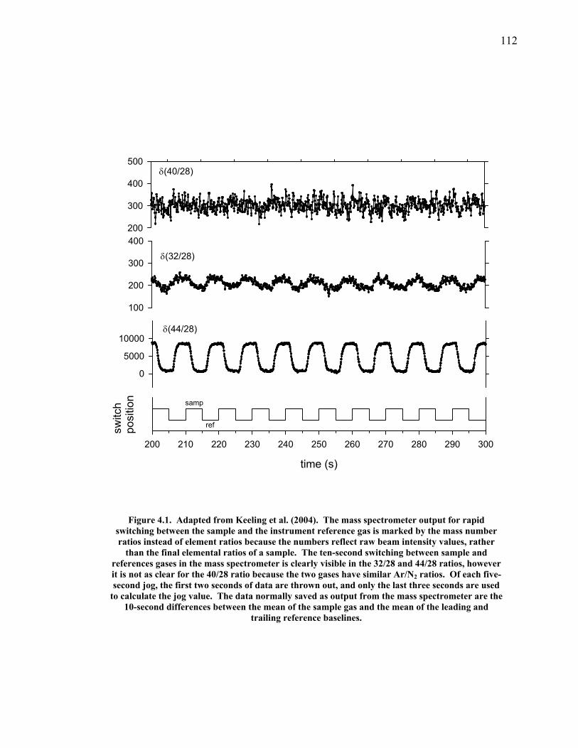
112
200
300
400
500δ(40/28)
100
200
300
400δ(32/28)
0
5000
10000δ(44/28)
time (s)
200 210 220 230 240 250 260 270 280 290 300
switc
hpo
sitio
n samp
ref
Figure 4.1. Adapted from Keeling et al. (2004). The mass spectrometer output for rapid switching between the sample and the instrument reference gas is marked by the mass number ratios instead of element ratios because the numbers reflect raw beam intensity values, rather
than the final elemental ratios of a sample. The ten-second switching between sample and references gases in the mass spectrometer is clearly visible in the 32/28 and 44/28 ratios, however it is not as clear for the 40/28 ratio because the two gases have similar Ar/N2 ratios. Of each five-second jog, the first two seconds of data are thrown out, and only the last three seconds are used
to calculate the jog value. The data normally saved as output from the mass spectrometer are the 10-second differences between the mean of the sample gas and the mean of the leading and
trailing reference baselines.
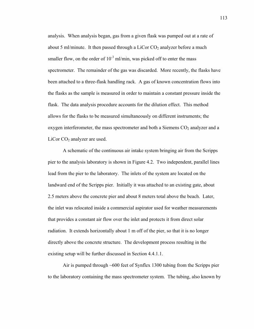
113
analysis. When analysis began, gas from a given flask was pumped out at a rate of
about 5 ml/minute. It then passed through a LiCor CO2 analyzer before a much
smaller flow, on the order of 10-3 ml/min, was picked off to enter the mass
spectrometer. The remainder of the gas was discarded. More recently, the flasks have
been attached to a three-flask handling rack. A gas of known concentration flows into
the flasks as the sample is measured in order to maintain a constant pressure inside the
flask. The data analysis procedure accounts for the dilution effect. This method
allows for the flasks to be measured simultaneously on different instruments; the
oxygen interferometer, the mass spectrometer and both a Siemens CO2 analyzer and a
LiCor CO2 analyzer are used.
A schematic of the continuous air intake system bringing air from the Scripps
pier to the analysis laboratory is shown in Figure 4.2. Two independent, parallel lines
lead from the pier to the laboratory. The inlets of the system are located on the
landward end of the Scripps pier. Initially it was attached to an existing gate, about
2.5 meters above the concrete pier and about 8 meters total above the beach. Later,
the inlet was relocated inside a commercial aspirator used for weather measurements
that provides a constant air flow over the inlet and protects it from direct solar
radiation. It extends horizontally about 1 m off of the pier, so that it is no longer
directly above the concrete structure. The development process resulting in the
existing setup will be further discussed in Section 4.4.1.1.
Air is pumped through ~600 feet of Synflex 1300 tubing from the Scripps pier
to the laboratory containing the mass spectrometer system. The tubing, also known by
114
Figure 4.2. Schematic of the continuous measurement system from the inlet on the pier through all laboratory instruments.
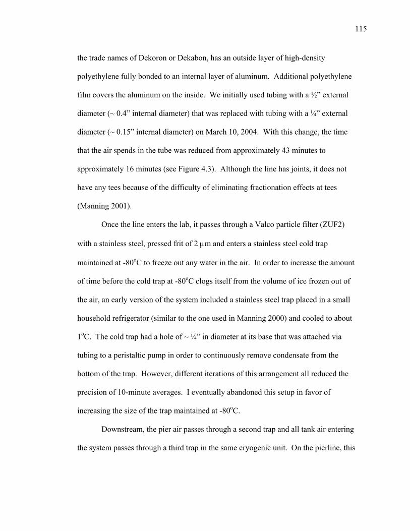
115
the trade names of Dekoron or Dekabon, has an outside layer of high-density
polyethylene fully bonded to an internal layer of aluminum. Additional polyethylene
film covers the aluminum on the inside. We initially used tubing with a ½” external
diameter (~ 0.4” internal diameter) that was replaced with tubing with a ¼” external
diameter (~ 0.15” internal diameter) on March 10, 2004. With this change, the time
that the air spends in the tube was reduced from approximately 43 minutes to
approximately 16 minutes (see Figure 4.3). Although the line has joints, it does not
have any tees because of the difficulty of eliminating fractionation effects at tees
(Manning 2001).
Once the line enters the lab, it passes through a Valco particle filter (ZUF2)
with a stainless steel, pressed frit of 2 μm and enters a stainless steel cold trap
maintained at -80oC to freeze out any water in the air. In order to increase the amount
of time before the cold trap at -80oC clogs itself from the volume of ice frozen out of
the air, an early version of the system included a stainless steel trap placed in a small
household refrigerator (similar to the one used in Manning 2000) and cooled to about
1oC. The cold trap had a hole of ~ ¼” in diameter at its base that was attached via
tubing to a peristaltic pump in order to continuously remove condensate from the
bottom of the trap. However, different iterations of this arrangement all reduced the
precision of 10-minute averages. I eventually abandoned this setup in favor of
increasing the size of the trap maintained at -80oC.
Downstream, the pier air passes through a second trap and all tank air entering
the system passes through a third trap in the same cryogenic unit. On the pierline, this
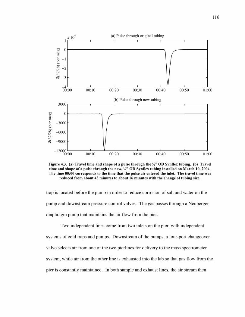
116
δ(32
/28)
(pe
r m
eg)
(a) Pulse through original tubing
00:00 00:10 00:20 00:30 00:40 00:50 01:00−4
−3
−2
−1
0
1x 10
4
δ(32
/28)
(pe
r m
eg)
(b) Pulse through new tubing
00:00 00:10 00:20 00:30 00:40 00:50 01:00−12000
−9000
−6000
−3000
0
3000
Figure 4.3. (a) Travel time and shape of a pulse through the ½” OD Synflex tubing. (b) Travel time and shape of a pulse through the new, ¼” OD Synflex tubing installed on March 10, 2004. The time 00:00 corresponds to the time that the pulse air entered the inlet. The travel time was
reduced from about 43 minutes to about 16 minutes with the change of tubing size.
trap is located before the pump in order to reduce corrosion of salt and water on the
pump and downstream pressure control valves. The gas passes through a Neuberger
diaphragm pump that maintains the air flow from the pier.
Two independent lines come from two inlets on the pier, with independent
systems of cold traps and pumps. Downstream of the pumps, a four-port changeover
valve selects air from one of the two pierlines for delivery to the mass spectrometer
system, while air from the other line is exhausted into the lab so that gas flow from the
pier is constantly maintained. In both sample and exhaust lines, the air stream then
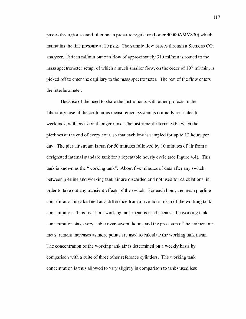
117
passes through a second filter and a pressure regulator (Porter 40000AMVS30) which
maintains the line pressure at 10 psig. The sample flow passes through a Siemens CO2
analyzer. Fifteen ml/min out of a flow of approximately 310 ml/min is routed to the
mass spectrometer setup, of which a much smaller flow, on the order of 10-3 ml/min, is
picked off to enter the capillary to the mass spectrometer. The rest of the flow enters
the interferometer.
Because of the need to share the instruments with other projects in the
laboratory, use of the continuous measurement system is normally restricted to
weekends, with occasional longer runs. The instrument alternates between the
pierlines at the end of every hour, so that each line is sampled for up to 12 hours per
day. The pier air stream is run for 50 minutes followed by 10 minutes of air from a
designated internal standard tank for a repeatable hourly cycle (see Figure 4.4). This
tank is known as the “working tank”. About five minutes of data after any switch
between pierline and working tank air are discarded and not used for calculations, in
order to take out any transient effects of the switch. For each hour, the mean pierline
concentration is calculated as a difference from a five-hour mean of the working tank
concentration. This five-hour working tank mean is used because the working tank
concentration stays very stable over several hours, and the precision of the ambient air
measurement increases as more points are used to calculate the working tank mean.
The concentration of the working tank air is determined on a weekly basis by
comparison with a suite of three other reference cylinders. The working tank
concentration is thus allowed to vary slightly in comparison to tanks used less
118
δ(40
/28)
(pe
r m
eg)
00:00 01:00 02:00 03:00 04:00 05:00−400
−300
−200
−100
0
100
200
Figure 4.4. Example of raw data output from the mass spectrometer. The left side shows the normal pierline run, with 50 minutes of pier air followed by 10 minutes of working tank air. The right side shows a run against three reference cylinders, with triplicate “jogs” of each reference tank against the working tank. Each “jog” consists of 10 minutes of a working tank baseline, 10 minutes of reference tank, and 10 minutes of a second working tank baseline. These reference
tanks are run once per week in order to determine the working tank concentration.
frequently. These reference tanks in turn are calibrated against a suite of other tanks
on 4-, 6- and 18-month cycles. The three reference tanks are run against the working
tank in a set of three, 10-minute jogs (see Figure 4.4). The lines are initially flushed
using a “fast purge”, and then during the test the tank air not presently selected
continues to be purged at a slower rate. If any of the three jogs differs statistically
from the mean, it is discarded and only two jogs are retained. Dedicated working
119
tanks last about 2-4 months for continuous measurements and are replaced when their
pressures fall below 200 psig.
Working tanks and reference tanks are filled with an oil-free compressor (RIX
Industries) and dried to below 5 μmoles mole-1 of H2O. Any adjustments in the
concentration needed for particular reference tanks are made by adding small amounts
of pure CO2, N2, O2. At this stage, none of the tanks are adjusted for Ar/N2. Tanks
are stored horizontally in an insulated box so that air is withdrawn from the vertical
center of the tank and temperature fluctuations are reduced.
4.3 Calibration
4.3.1 Establishing Ion Sensitivities
The mass spectrometer output consists of a voltage that is related to the actual
atmospheric abundances of certain masses. The process of deriving the atmospheric
abundance ratios from this signal output involves several steps that take into account
interferences from other atmospheric species, nonlinearities of the system, and regular
comparison with reference gases (mentioned in the previous section). Following
Keeling et al. (2004), these effects can be described by the equations:
( ) ( ) ( ) ,28322840 121112 DCOCBANAr +Δ++= δδδ and (4.2)
( ) ( ) ( ) ,28402832 2222222 DCOCBANO +Δ++= δδδ (4.3)
where A represents nonlinearities, B and C represent interferences, and D represents
changes in the instrument reference gas, laboratory reference gases, and working tank
gases. The ratios are written as mass number ratios (e.g. δ(40/28)) to represent the
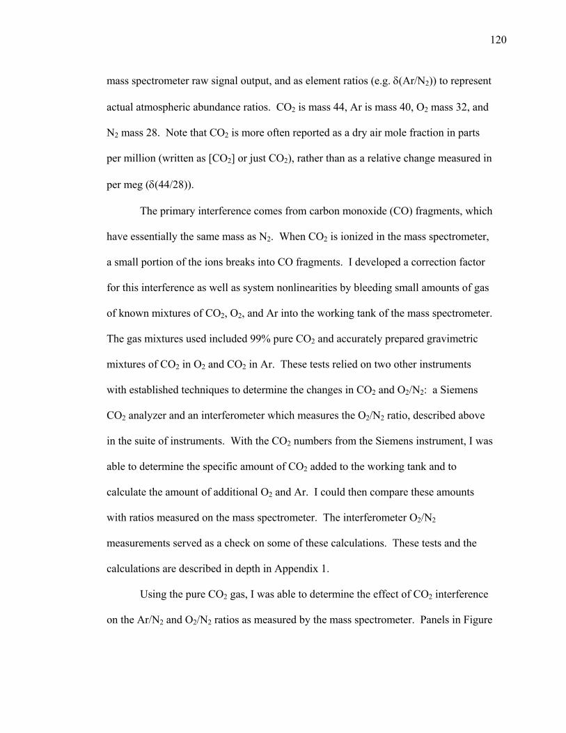
120
mass spectrometer raw signal output, and as element ratios (e.g. δ(Ar/N2)) to represent
actual atmospheric abundance ratios. CO2 is mass 44, Ar is mass 40, O2 mass 32, and
N2 mass 28. Note that CO2 is more often reported as a dry air mole fraction in parts
per million (written as [CO2] or just CO2), rather than as a relative change measured in
per meg (δ(44/28)).
The primary interference comes from carbon monoxide (CO) fragments, which
have essentially the same mass as N2. When CO2 is ionized in the mass spectrometer,
a small portion of the ions breaks into CO fragments. I developed a correction factor
for this interference as well as system nonlinearities by bleeding small amounts of gas
of known mixtures of CO2, O2, and Ar into the working tank of the mass spectrometer.
The gas mixtures used included 99% pure CO2 and accurately prepared gravimetric
mixtures of CO2 in O2 and CO2 in Ar. These tests relied on two other instruments
with established techniques to determine the changes in CO2 and O2/N2: a Siemens
CO2 analyzer and an interferometer which measures the O2/N2 ratio, described above
in the suite of instruments. With the CO2 numbers from the Siemens instrument, I was
able to determine the specific amount of CO2 added to the working tank and to
calculate the amount of additional O2 and Ar. I could then compare these amounts
with ratios measured on the mass spectrometer. The interferometer O2/N2
measurements served as a check on some of these calculations. These tests and the
calculations are described in depth in Appendix 1.
Using the pure CO2 gas, I was able to determine the effect of CO2 interference
on the Ar/N2 and O2/N2 ratios as measured by the mass spectrometer. Panels in Figure
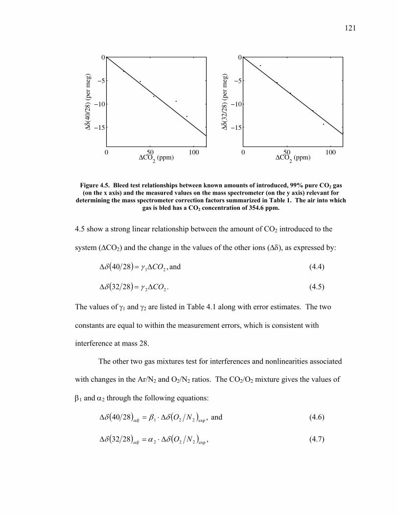
121
ΔCO2 (ppm)
Δδ(4
0/28
) (p
er m
eg)
0 50 100
−15
−10
−5
0
ΔCO2 (ppm)
Δδ(3
2/28
) (p
er m
eg)
0 50 100
−15
−10
−5
0
Figure 4.5. Bleed test relationships between known amounts of introduced, 99% pure CO2 gas (on the x axis) and the measured values on the mass spectrometer (on the y axis) relevant for
determining the mass spectrometer correction factors summarized in Table 1. The air into which gas is bled has a CO2 concentration of 354.6 ppm.
4.5 show a strong linear relationship between the amount of CO2 introduced to the
system (ΔCO2) and the change in the values of the other ions (Δδ), as expressed by:
( ) ,2840 21 COΔ=Δ γδ and (4.4)
( ) .2832 22 COΔ=Δ γδ (4.5)
The values of γ1 and γ2 are listed in Table 4.1 along with error estimates. The two
constants are equal to within the measurement errors, which is consistent with
interference at mass 28.
The other two gas mixtures test for interferences and nonlinearities associated
with changes in the Ar/N2 and O2/N2 ratios. The CO2/O2 mixture gives the values of
β1 and α2 through the following equations:
( ) ( ) ,2840 exp221 NOadj δβδ Δ⋅=Δ and (4.6)
( ) ( ) ,2832 exp222 NOadj δαδ Δ⋅=Δ (4.7)
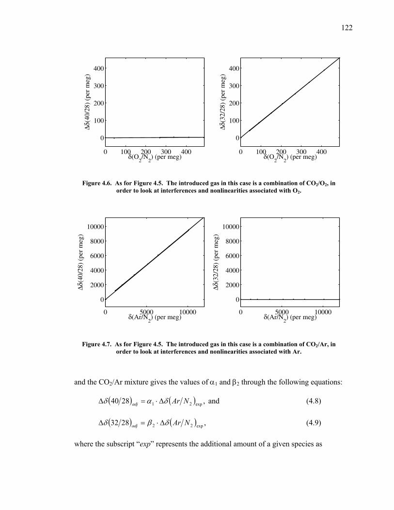
122
Δδ(4
0/28
) (p
er m
eg)
δ(O2/N
2) (per meg)
0 100 200 300 400
0
100
200
300
400
Δδ(3
2/28
) (p
er m
eg)
δ(O2/N
2) (per meg)
0 100 200 300 400
0
100
200
300
400
Figure 4.6. As for Figure 4.5. The introduced gas in this case is a combination of CO2/O2, in order to look at interferences and nonlinearities associated with O2.
Δδ(4
0/28
) (p
er m
eg)
δ(Ar/N2) (per meg)
0 5000 10000
0
2000
4000
6000
8000
10000
Δδ(3
2/28
) (p
er m
eg)
δ(Ar/N2) (per meg)
0 5000 10000
0
2000
4000
6000
8000
10000
Figure 4.7. As for Figure 4.5. The introduced gas in this case is a combination of CO2/Ar, in order to look at interferences and nonlinearities associated with Ar.
and the CO2/Ar mixture gives the values of α1 and β2 through the following equations:
( ) ( ) ,2840 exp21 NAradj δαδ Δ⋅=Δ and (4.8)
( ) ( ) ,2832 exp22 NAradj δβδ Δ⋅=Δ (4.9)
where the subscript “exp” represents the additional amount of a given species as
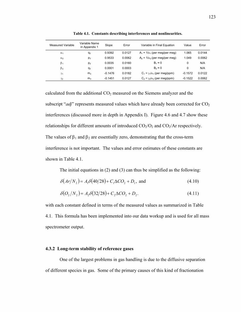
123
Table 4.1. Constants describing interferences and nonlinearities.
Measured Variable Variable Name in Appendix 1 Slope Error Variable in Final Equation Value Error
α1 q2 0.9392 0.0127 A1 = 1/α1 (per meg/per meg) 1.065 0.0144
α2 p3 0.9533 0.0062 A2 = 1/α2 (per meg/per meg) 1.049 0.0062
β1 p2 0.0035 0.0160 B1 ≈ 0 0 N/A
β2 q3 0.0001 0.0003 B2 ≈ 0 0 N/A
γ1 m2 -0.1476 0.0182 C1 = γ1/α1 (per meg/ppm) -0.1572 0.0122
γ2 m3 -0.1451 0.0127 C2 = γ2/α2 (per meg/ppm) -0.1522 0.0062
calculated from the additional CO2 measured on the Siemens analyzer and the
subscript “adj” represents measured values which have already been corrected for CO2
interferences (discussed more in depth in Appendix I). Figure 4.6 and 4.7 show these
relationships for different amounts of introduced CO2/O2 and CO2/Ar respectively.
The values of β1 and β2 are essentially zero, demonstrating that the cross-term
interference is not important. The values and error estimates of these constants are
shown in Table 4.1.
The initial equations in (2) and (3) can thus be simplified as the following:
( ) ( ) ,2840 12112 DCOCANAr +Δ+= δδ and (4.10)
( ) ( ) .2832 222222 DCOCANO +Δ+= δδ (4.11)
with each constant defined in terms of the measured values as summarized in Table
4.1. This formula has been implemented into our data workup and is used for all mass
spectrometer output.
4.3.2 Long-term stability of reference gases
One of the largest problems in gas handling is due to the diffusive separation
of different species in gas. Some of the primary causes of this kind of fractionation
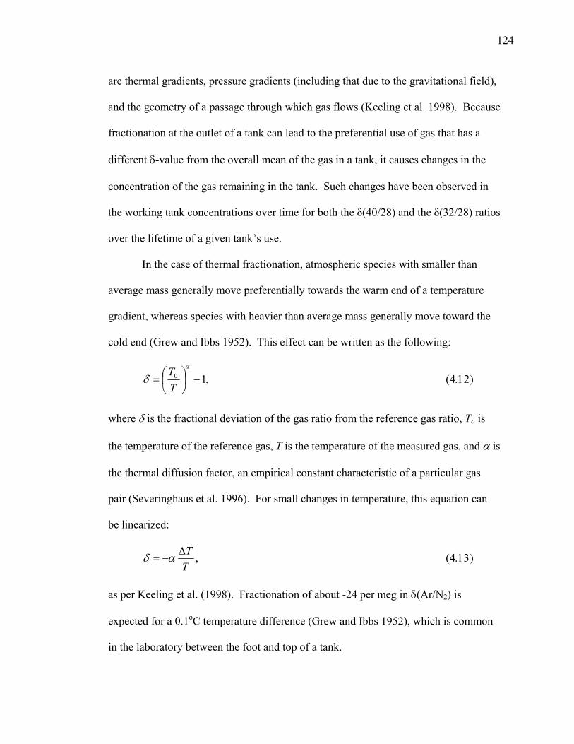
124
are thermal gradients, pressure gradients (including that due to the gravitational field),
and the geometry of a passage through which gas flows (Keeling et al. 1998). Because
fractionation at the outlet of a tank can lead to the preferential use of gas that has a
different δ-value from the overall mean of the gas in a tank, it causes changes in the
concentration of the gas remaining in the tank. Such changes have been observed in
the working tank concentrations over time for both the δ(40/28) and the δ(32/28) ratios
over the lifetime of a given tank’s use.
In the case of thermal fractionation, atmospheric species with smaller than
average mass generally move preferentially towards the warm end of a temperature
gradient, whereas species with heavier than average mass generally move toward the
cold end (Grew and Ibbs 1952). This effect can be written as the following:
,10 −⎟⎠⎞
⎜⎝⎛=
α
δTT
(4.12)
where δ is the fractional deviation of the gas ratio from the reference gas ratio, To is
the temperature of the reference gas, T is the temperature of the measured gas, and α is
the thermal diffusion factor, an empirical constant characteristic of a particular gas
pair (Severinghaus et al. 1996). For small changes in temperature, this equation can
be linearized:
,TTΔ
−= αδ (4.13)
as per Keeling et al. (1998). Fractionation of about -24 per meg in δ(Ar/N2) is
expected for a 0.1oC temperature difference (Grew and Ibbs 1952), which is common
in the laboratory between the foot and top of a tank.
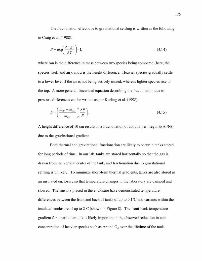
125
The fractionation effect due to gravitational settling is written as the following
in Craig et al. (1988):
,1exp −⎟⎠⎞
⎜⎝⎛ Δ
=RTmgzδ (4.14)
where Δm is the difference in mass between two species being compared (here, the
species itself and air), and z is the height difference. Heavier species gradually settle
to a lower level if the air is not being actively mixed, whereas lighter species rise to
the top. A more general, linearized equation describing the fractionation due to
pressure differences can be written as per Keeling et al. (1998):
⎟⎠⎞
⎜⎝⎛ Δ
⎟⎟⎠
⎞⎜⎜⎝
⎛ −=
PP
mmm
air
NAr 2δ . (4.15)
A height difference of 10 cm results in a fractionation of about 5 per meg in δ(Ar/N2)
due to the gravitational gradient.
Both thermal and gravitational fractionation are likely to occur in tanks stored
for long periods of time. In our lab, tanks are stored horizontally so that the gas is
drawn from the vertical center of the tank, and fractionation due to gravitational
settling is unlikely. To minimize short-term thermal gradients, tanks are also stored in
an insulated enclosure so that temperature changes in the laboratory are damped and
slowed. Thermistors placed in the enclosure have demonstrated temperature
differences between the front and back of tanks of up to 0.1oC and variants within the
insulated enclosure of up to 2oC (shown in Figure 8). The front-back temperature
gradient for a particular tank is likely important in the observed reduction in tank
concentration of heavier species such as Ar and O2 over the lifetime of the tank.
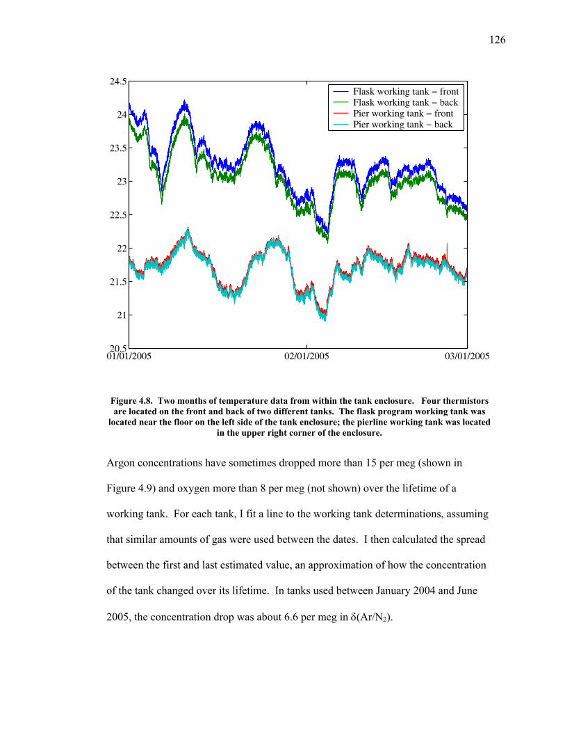
126
01/01/2005 02/01/2005 03/01/200520.5
21
21.5
22
22.5
23
23.5
24
24.5Flask working tank − frontFlask working tank − backPier working tank − frontPier working tank − back
Figure 4.8. Two months of temperature data from within the tank enclosure. Four thermistors are located on the front and back of two different tanks. The flask program working tank was
located near the floor on the left side of the tank enclosure; the pierline working tank was located in the upper right corner of the enclosure.
Argon concentrations have sometimes dropped more than 15 per meg (shown in
Figure 4.9) and oxygen more than 8 per meg (not shown) over the lifetime of a
working tank. For each tank, I fit a line to the working tank determinations, assuming
that similar amounts of gas were used between the dates. I then calculated the spread
between the first and last estimated value, an approximation of how the concentration
of the tank changed over its lifetime. In tanks used between January 2004 and June
2005, the concentration drop was about 6.6 per meg in δ(Ar/N2).
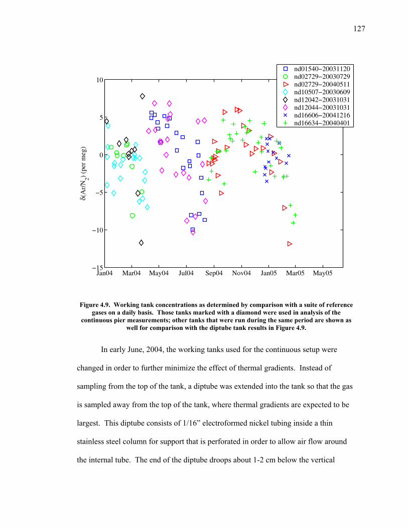
127
δ(A
r/N
2) (p
er m
eg)
Jan04 Mar04 May04 Jul04 Sep04 Nov04 Jan05 Mar05 May05−15
−10
−5
0
5
10
nd01540−20031120nd02729−20030729nd02729−20040511nd10507−20030609nd12042−20031031nd12044−20031031nd16606−20041216nd16634−20040401
Figure 4.9. Working tank concentrations as determined by comparison with a suite of reference
gases on a daily basis. Those tanks marked with a diamond were used in analysis of the continuous pier measurements; other tanks that were run during the same period are shown as
well for comparison with the diptube tank results in Figure 4.9.
In early June, 2004, the working tanks used for the continuous setup were
changed in order to further minimize the effect of thermal gradients. Instead of
sampling from the top of the tank, a diptube was extended into the tank so that the gas
is sampled away from the top of the tank, where thermal gradients are expected to be
largest. This diptube consists of 1/16” electroformed nickel tubing inside a thin
stainless steel column for support that is perforated in order to allow air flow around
the internal tube. The end of the diptube droops about 1-2 cm below the vertical
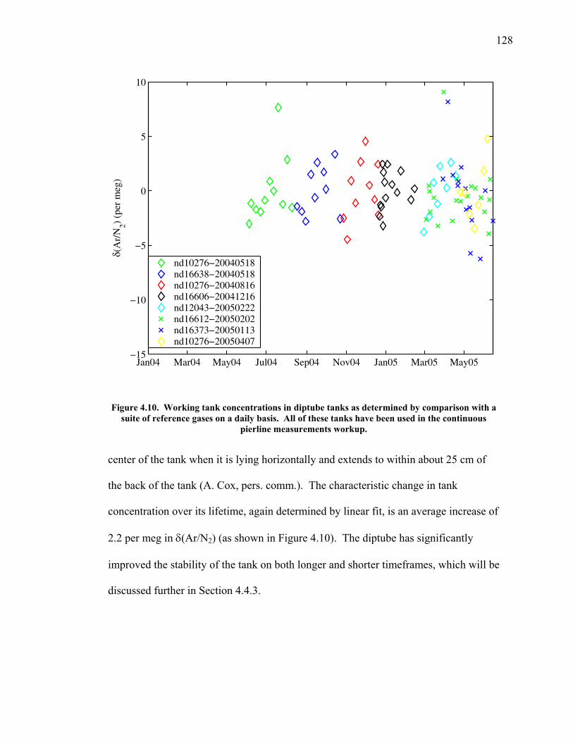
128
δ(A
r/N
2) (p
er m
eg)
Jan04 Mar04 May04 Jul04 Sep04 Nov04 Jan05 Mar05 May05−15
−10
−5
0
5
10
nd10276−20040518nd16638−20040518nd10276−20040816nd16606−20041216nd12043−20050222nd16612−20050202nd16373−20050113nd10276−20050407
Figure 4.10. Working tank concentrations in diptube tanks as determined by comparison with a suite of reference gases on a daily basis. All of these tanks have been used in the continuous
pierline measurements workup.
center of the tank when it is lying horizontally and extends to within about 25 cm of
the back of the tank (A. Cox, pers. comm.). The characteristic change in tank
concentration over its lifetime, again determined by linear fit, is an average increase of
2.2 per meg in δ(Ar/N2) (as shown in Figure 4.10). The diptube has significantly
improved the stability of the tank on both longer and shorter timeframes, which will be
discussed further in Section 4.4.3.
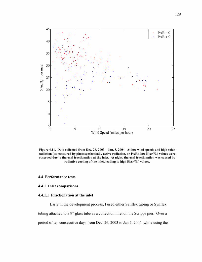
129
Wind Speed (miles per hour)
δ(A
r/N
2) (p
er m
eg)
0 5 10 15 20 255
10
15
20
25
30
35
40
45PAR ~ 0PAR > 0
Figure 4.11. Data collected from Dec. 26, 2003 – Jan. 5, 2004. At low wind speeds and high solar radiation (as measured by photosynthetically active radiation, or PAR), low δ(Ar/N2) values were observed due to thermal fractionation at the inlet. At night, thermal fractionation was caused by
radiative cooling of the inlet, leading to high δ(Ar/N2) values.
4.4 Performance tests
4.4.1 Inlet comparisons
4.4.1.1 Fractionation at the inlet
Early in the development process, I used either Synflex tubing or Synflex
tubing attached to a 9” glass tube as a collection inlet on the Scripps pier. Over a
period of ten consecutive days from Dec. 26, 2003 to Jan 5, 2004, while using the
130
glass inlet, the measured δ(Ar/N2) concentration varied 40 per meg. High values were
correlated with low winds and no solar radiation; low values were correlated with low
winds and strong solar radiation. During periods when the wind speed climbed above
10 miles per hour, the values during low and high solar radiation were much more
consistent (see Figure 4.11). These results suggest that thermal fractionation at the
inlet are causing these fluctuations. During the day when the inlet is heated by solar
radiation, thermal fractionation would lead to lower δ(Ar/N2) values, whereas at
night, when the inlet cools radiatively, thermal fractionation would lead to higher
δ(Ar/N2) values.
In order to prevent thermal fractionation near the inlet, I installed the pierline
inlet inside an aspirated radiation shield (R.M. Young 43408) commonly used in
weather stations to protect instruments from solar heating. Formed of two concentric
intake tubes with a canopy shade, a blower at the end of the pipe generates a flow of
3.4-7.6 meters per second through the intake tubes and across any sensor. Instead of a
meterological sensor, I have placed Synflex tubing inside the aspirator intake tubes,
with the tubing end located approximately 2” above the base of the intake tubes (see
Figure 4.2) and exiting the junction box at the top of the radiation shield.
I tested this new setup by switching on an hourly basis between two lines with
different inlet systems. The end of one Synflex pierline was placed inside the intake
tube of the aspirator as described above. The other Synflex pierline was left
unprotected. Over a period of 24 hours, the aspirated line showed a constant δ(Ar/N2)
concentration, whereas the concentration in the unprotected line dropped by up to 80
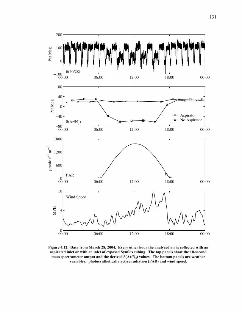
131
Per
Meg
δ(40/28)
00:00 06:00 12:00 18:00 00:00−100
0
100
200
Per
Meg
δ(Ar/N2)
00:00 06:00 12:00 18:00 00:00−80
−40
0
40
80
μmol
e s−
1 m−
2
PAR
00:00 06:00 12:00 18:00 00:000
600
1200
1800
MPH
Wind Speed
00:00 06:00 12:00 18:00 00:000
5
10
AspiratorNo Aspirator
Figure 4.12. Data from March 28, 2004. Every other hour the analyzed air is collected with an aspirated inlet or with an inlet of exposed Synflex tubing. The top panels show the 10-second mass spectrometer output and the derived δ(Ar/N2) values. The bottom panels are weather
variables: photosynthetically active radiation (PAR) and wind speed.
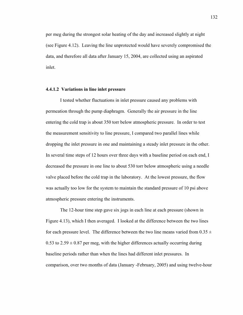
132
per meg during the strongest solar heating of the day and increased slightly at night
(see Figure 4.12). Leaving the line unprotected would have severely compromised the
data, and therefore all data after January 15, 2004, are collected using an aspirated
inlet.
4.4.1.2 Variations in line inlet pressure
I tested whether fluctuations in inlet pressure caused any problems with
permeation through the pump diaphragm. Generally the air pressure in the line
entering the cold trap is about 350 torr below atmospheric pressure. In order to test
the measurement sensitivity to line pressure, I compared two parallel lines while
dropping the inlet pressure in one and maintaining a steady inlet pressure in the other.
In several time steps of 12 hours over three days with a baseline period on each end, I
decreased the pressure in one line to about 530 torr below atmospheric using a needle
valve placed before the cold trap in the laboratory. At the lowest pressure, the flow
was actually too low for the system to maintain the standard pressure of 10 psi above
atmospheric pressure entering the instruments.
The 12-hour time step gave six jogs in each line at each pressure (shown in
Figure 4.13), which I then averaged. I looked at the difference between the two lines
for each pressure level. The difference between the two line means varied from 0.35 ±
0.53 to 2.59 ± 0.87 per meg, with the higher differences actually occurring during
baseline periods rather than when the lines had different inlet pressures. In
comparison, over two months of data (January -February, 2005) and using twelve-hour
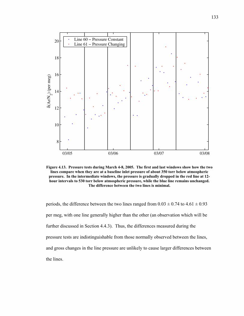
133
δ(A
r/N
2) (p
er m
eg)
03/05 03/06 03/07 03/08
8
10
12
14
16
18
20 Line 60 − Pressure ConstantLine 61 − Pressure Changing
Figure 4.13. Pressure tests during March 4-8, 2005. The first and last windows show how the two
lines compare when they are at a baseline inlet pressure of about 350 torr below atmospheric pressure. In the intermediate windows, the pressure is gradually dropped in the red line at 12-hour intervals to 530 torr below atmospheric pressure, while the blue line remains unchanged.
The difference between the two lines is minimal.
periods, the difference between the two lines ranged from 0.03 ± 0.74 to 4.61 ± 0.93
per meg, with one line generally higher than the other (an observation which will be
further discussed in Section 4.4.3). Thus, the differences measured during the
pressure tests are indistinguishable from those normally observed between the lines,
and gross changes in the line pressure are unlikely to cause larger differences between
the lines.
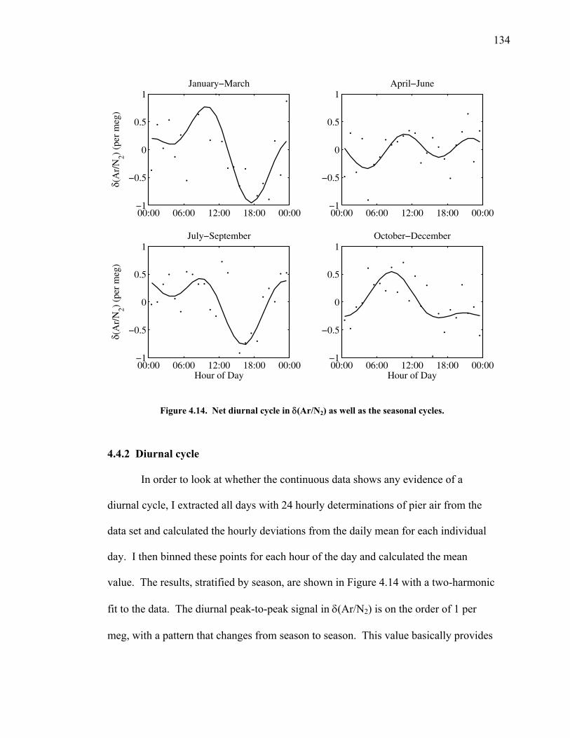
134
January−March
δ(A
r/N
2) (p
er m
eg)
00:00 06:00 12:00 18:00 00:00−1
−0.5
0
0.5
1April−June
00:00 06:00 12:00 18:00 00:00−1
−0.5
0
0.5
1
July−September
δ(A
r/N
2) (p
er m
eg)
Hour of Day00:00 06:00 12:00 18:00 00:00−1
−0.5
0
0.5
1October−December
Hour of Day00:00 06:00 12:00 18:00 00:00−1
−0.5
0
0.5
1
Figure 4.14. Net diurnal cycle in δ(Ar/N2) as well as the seasonal cycles.
4.4.2 Diurnal cycle
In order to look at whether the continuous data shows any evidence of a
diurnal cycle, I extracted all days with 24 hourly determinations of pier air from the
data set and calculated the hourly deviations from the daily mean for each individual
day. I then binned these points for each hour of the day and calculated the mean
value. The results, stratified by season, are shown in Figure 4.14 with a two-harmonic
fit to the data. The diurnal peak-to-peak signal in δ(Ar/N2) is on the order of 1 per
meg, with a pattern that changes from season to season. This value basically provides
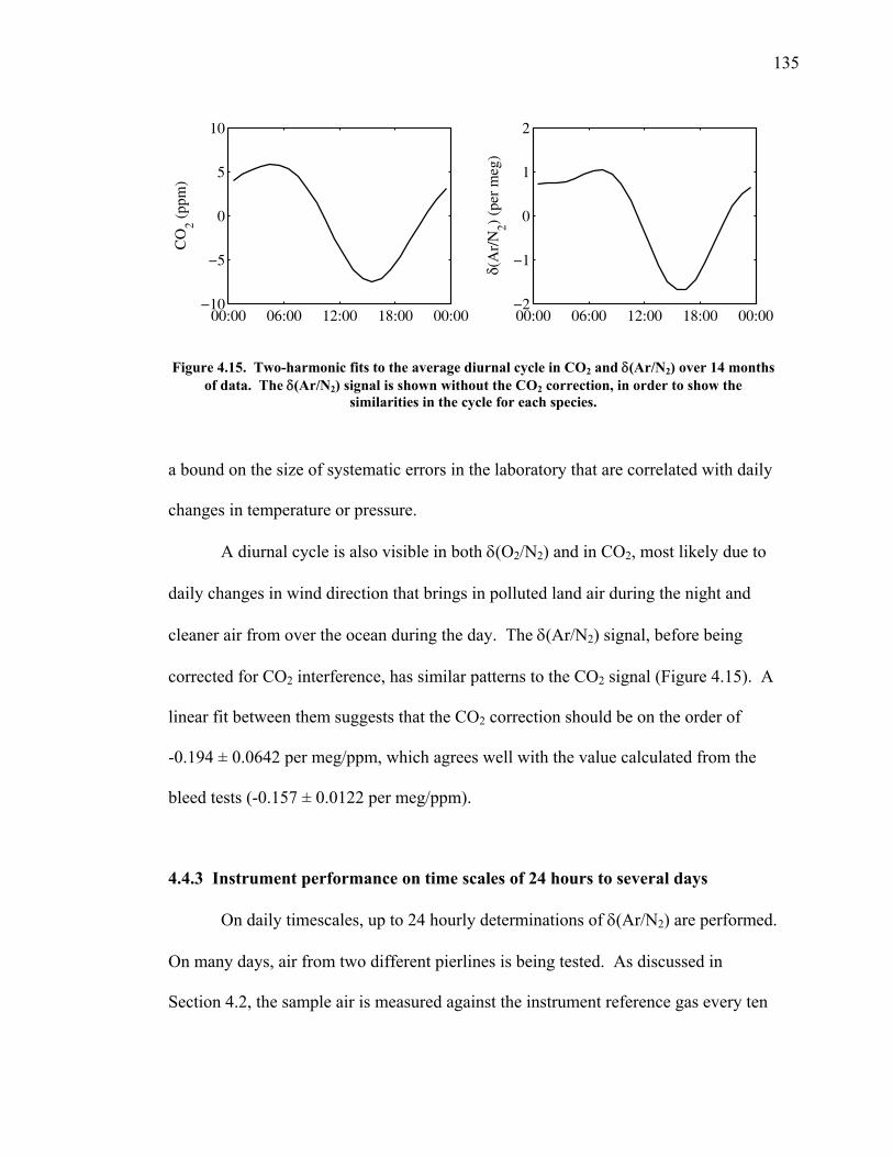
135
CO
2 (pp
m)
00:00 06:00 12:00 18:00 00:00−10
−5
0
5
10
δ(A
r/N
2) (p
er m
eg)
00:00 06:00 12:00 18:00 00:00−2
−1
0
1
2
Figure 4.15. Two-harmonic fits to the average diurnal cycle in CO2 and δ(Ar/N2) over 14 months
of data. The δ(Ar/N2) signal is shown without the CO2 correction, in order to show the similarities in the cycle for each species.
a bound on the size of systematic errors in the laboratory that are correlated with daily
changes in temperature or pressure.
A diurnal cycle is also visible in both δ(O2/N2) and in CO2, most likely due to
daily changes in wind direction that brings in polluted land air during the night and
cleaner air from over the ocean during the day. The δ(Ar/N2) signal, before being
corrected for CO2 interference, has similar patterns to the CO2 signal (Figure 4.15). A
linear fit between them suggests that the CO2 correction should be on the order of
-0.194 ± 0.0642 per meg/ppm, which agrees well with the value calculated from the
bleed tests (-0.157 ± 0.0122 per meg/ppm).
4.4.3 Instrument performance on time scales of 24 hours to several days
On daily timescales, up to 24 hourly determinations of δ(Ar/N2) are performed.
On many days, air from two different pierlines is being tested. As discussed in
Section 4.2, the sample air is measured against the instrument reference gas every ten
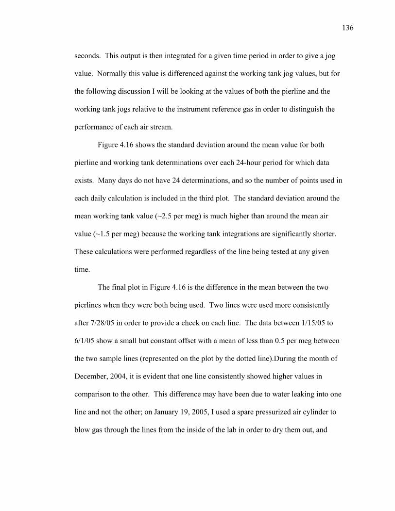
136
seconds. This output is then integrated for a given time period in order to give a jog
value. Normally this value is differenced against the working tank jog values, but for
the following discussion I will be looking at the values of both the pierline and the
working tank jogs relative to the instrument reference gas in order to distinguish the
performance of each air stream.
Figure 4.16 shows the standard deviation around the mean value for both
pierline and working tank determinations over each 24-hour period for which data
exists. Many days do not have 24 determinations, and so the number of points used in
each daily calculation is included in the third plot. The standard deviation around the
mean working tank value (~2.5 per meg) is much higher than around the mean air
value (~1.5 per meg) because the working tank integrations are significantly shorter.
These calculations were performed regardless of the line being tested at any given
time.
The final plot in Figure 4.16 is the difference in the mean between the two
pierlines when they were both being used. Two lines were used more consistently
after 7/28/05 in order to provide a check on each line. The data between 1/15/05 to
6/1/05 show a small but constant offset with a mean of less than 0.5 per meg between
the two sample lines (represented on the plot by the dotted line).During the month of
December, 2004, it is evident that one line consistently showed higher values in
comparison to the other. This difference may have been due to water leaking into one
line and not the other; on January 19, 2005, I used a spare pressurized air cylinder to
blow gas through the lines from the inside of the lab in order to dry them out, and
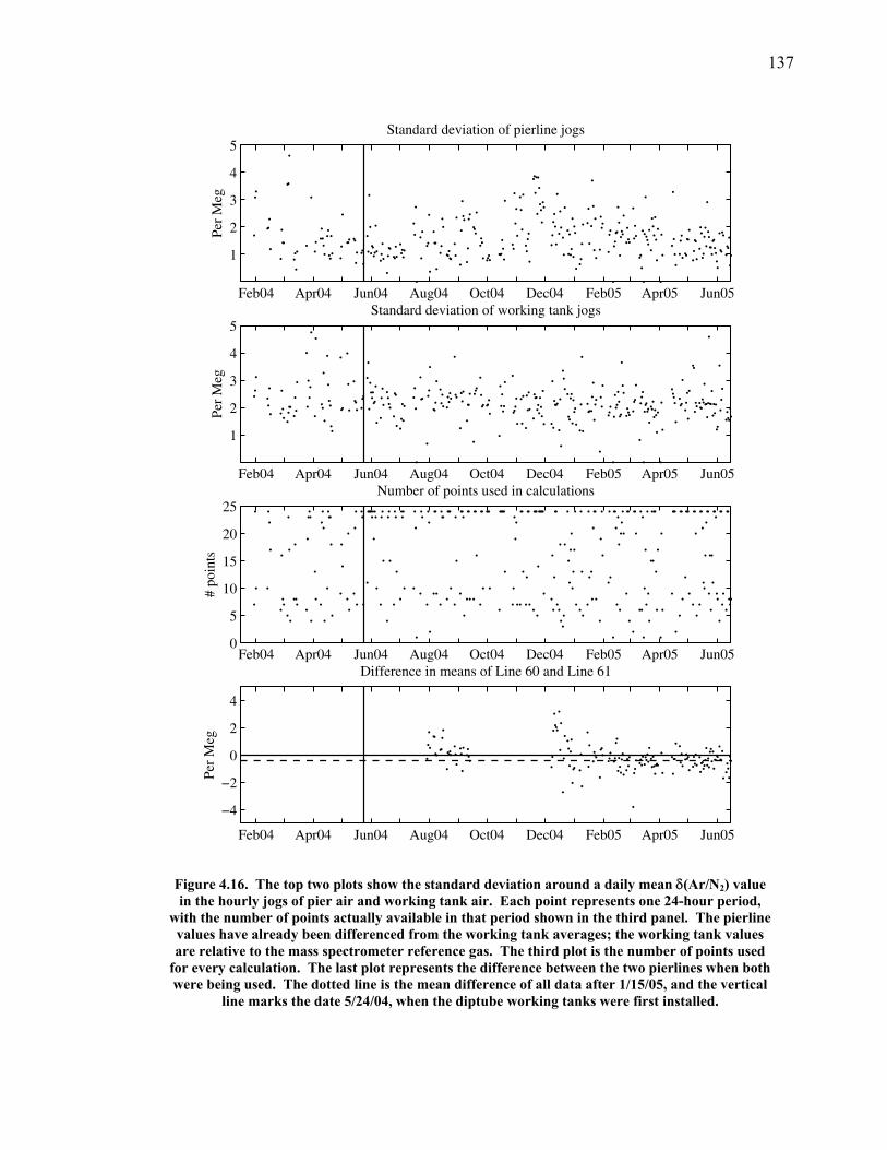
137
Per
Meg
Standard deviation of pierline jogs
Feb04 Apr04 Jun04 Aug04 Oct04 Dec04 Feb05 Apr05 Jun05
1
2
3
4
5
Per
Meg
Standard deviation of working tank jogs
Feb04 Apr04 Jun04 Aug04 Oct04 Dec04 Feb05 Apr05 Jun05
1
2
3
4
5
# po
ints
Number of points used in calculations
Feb04 Apr04 Jun04 Aug04 Oct04 Dec04 Feb05 Apr05 Jun050
5
10
15
20
25
Per
Meg
Difference in means of Line 60 and Line 61
Feb04 Apr04 Jun04 Aug04 Oct04 Dec04 Feb05 Apr05 Jun05
−4
−2
0
2
4
Figure 4.16. The top two plots show the standard deviation around a daily mean δ(Ar/N2) value in the hourly jogs of pier air and working tank air. Each point represents one 24-hour period,
with the number of points actually available in that period shown in the third panel. The pierline values have already been differenced from the working tank averages; the working tank values are relative to the mass spectrometer reference gas. The third plot is the number of points used
for every calculation. The last plot represents the difference between the two pierlines when both were being used. The dotted line is the mean difference of all data after 1/15/05, and the vertical
line marks the date 5/24/04, when the diptube working tanks were first installed.
138
Per
Meg
Standard deviation of pierline jogs
Feb04 Apr04 Jun04 Aug04 Oct04 Dec04 Feb05 Apr05 Jun05
1
2
3
4
5
Per
Meg
Standard deviation of working tank jogs
Feb04 Apr04 Jun04 Aug04 Oct04 Dec04 Feb05 Apr05 Jun05
1
2
3
4
5
# po
ints
Number of points used in calculations
Feb04 Apr04 Jun04 Aug04 Oct04 Dec04 Feb05 Apr05 Jun050
50
100
150
200
Per
Meg
Difference in means of Line 60 and Line 61
Feb04 Apr04 Jun04 Aug04 Oct04 Dec04 Feb05 Apr05 Jun05
−4
−2
0
2
4
Figure 4.17. As for Figure 5.15, except each point represents each period the pierline was run before being turned off. The time represented by each point can range from 1-8 days. In the working tank jogs, the daily average standard deviation (in Figure 5.15) stayed fairly constant
over the entire record.
139
about 10 mls of water came out of one of the lines. Any openings around the aspirator
fittings were also filled in at this time.
Because it is worth looking at possible drift on timescales greater than one day,
Figure 4.17 show similar calculations using each weekend of data rather than each 24-
hour period. Although the plot showing the standard deviation of pierline jogs is
similar to the plot in Figure 4.16, the plot showing the working tank jogs is different.
There is a clear shift in the standard deviation from before to after the installation of a
diptube in the working tanks on 5/24/04. In the later data, the standard deviation over
each period when the pierline was run consistently (up to several days) drops to about
the same standard deviation as during a 24-hour period. This observation strengthens
the argument for using diptube working tanks in order to obtain more stable working
tank concentrations on the order of days to months.
4.5 Comparison of flask and continuous sampling of δ(Ar/N2) at La Jolla
Figure 4.16 shows data from the first 17 months of continuous sampling for
δ(Ar/N2) at La Jolla, along with all flask measurements during the same period. Also
plotted is the first harmonic fit to the seasonal cycle of the continuous measurements.
It must be noted that the zero on this scale is arbitrary, because it represents an average
of a set of standard gases of unknown composition.
Although these continuous measurements will be discussed in depth in a subsequent
chapter of this thesis, it is immediately clear that the continuous data resolve the
seasonal cycle much better than the flask measurements. Of the two flask
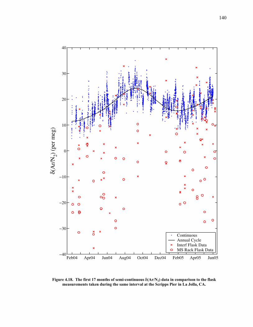
140
δ(A
r/N
2) (
per
meg
)
Feb04 Apr04 Jun04 Aug04 Oct04 Dec04 Feb05 Apr05 Jun05−40
−30
−20
−10
0
10
20
30
40
ContinuousAnnual CycleInterf Flask DataMS Rack Flask Data
Figure 4.18. The first 17 months of semi-continuous δ(Ar/N2) data in comparison to the flask measurements taken during the same interval at the Scripps Pier in La Jolla, CA.
141
analysis techniques, one (Interf) has an annual mean which agrees better with the
continuous measurements, whereas the other (MS Rack) shows a significant difference
in mean value. This observation raises the question whether the continuous
measurements still have some bias, in which the annual mean is higher relative to the
flask measurements than it should be. However, it is also likely that the flask
measurements have a fractionation bias, most likely towards lighter (or lower) values,
because the flasks are sampled in the middle of the day without an aspirator.
The continuous record also shows much more temporal detail. The δ(Ar/N2)
concentration can deviate up to 10 per meg from the fitted seasonal cycle on the order
of 1-3 weeks, which is larger than the size of the annual cycle. It is to be hoped that
these measurements will give more insight into short-term variability of the δ(Ar/N2)
that has not been previously observed.
4.6 Conclusions
In this chapter, I described a new gas handling system to perform continuous
measurements of the Ar/N2 ratio at the Scripps pier in La Jolla. One-hour averages of
a continuous air stream have a precision of 2-3 per meg and are well within the
necessary precision to detect the expected seasonal changes in the Ar/N2 ratio.
The main key to obtaining the precision necessary for measurements of the
seasonal cycle was the reduction of thermal fractionation at the collection inlet.
Introduction of a commercially available aspirator provides a constantly mixed air
stream, which prevents fractionated gases from forming near the inlet. The aspirator
142
reduced the spread of hourly values over several days from 40 per meg to 8-15 per
meg. Given the number of hourly determinations, such a precision permits detection
of a seasonal cycle with an amplitude of about 8 per meg. In contrast, although the
imprecision on the mean of three flask samples collected together is most likely about
±11 per meg, real differences between flasks can show a spread of 45 per meg
(Keeling et al. 2004). The net change in the concentration of the working tanks over
the lifetime of the tank also has been significantly reduced with the introduction of
diptube tanks. Better insulation from thermal changes in the laboratory may improve
the stability even further.
The continuous data show variability on the order of a few weeks that has
never been observed and which may yield insight into geochemical controls on
δ(Ar/N2). Alternatively, it may represent a previously unrecognized laboratory
artifact. This variability will be further discussed in a subsequent chapter.
143
4.7 Bibliography
Battle, M., M. Bender, M. B. Hendricks, D. T. Ho, R. Mika, G. McKinley, S.-M. Fan,
T. Blaine, and R. F. Keeling. 2003. Measurements and models of the atmospheric Ar/N2 ratio. Geophys. Res. Lett. 30 (doi: 10.1029/2003GL017411).
Bender, M. L., P. P. Tans, J. T. Ellis, J. Orchardo, and K. Habfast. 1994. A high
precision isotope ratio mass spectrometry method for measuring the O2/N2 ratio of air. Geochim. Cosmochim. Ac. 58: 4751-4758.
Craig, H., Y. Horibe, and T. Sowers. 1988. Gravitational separation of gases and
isotopes in polar ice caps. Science 242: 1675-1678. Grew, K. E. And T. L. Ibbs. 1952. Thermal Diffusion in Gases. Cambridge
University Press: New York. Keeling, R. F., T. Blaine, B. Paplawsky, L. Katz, C. Atwood, and T. Brockwell. 2004.
Measurement of changes in atmospheric Ar/N2 ratio using a rapid-switching, single-capillary mass spectrometer system. Tellus 56B: 322-388.
Keeling, R. F., A. C. Manning, E. M. McEvoy, and S. R. Shertz. 1998. Methods for
measuring changes in atmospheric O2 concentration and their application in southern hemisphere air. J. Geophys. Res. 103: 3381-3397.
Manning, Andrew C. 2001. Temporal variability of atmospheric oxygen from both
continuous measurements and a flask sampling network: Tools for studying the global carbon cycle. Ph.D. thesis: University of California, San Diego.
Severinghaus, J. P., M. L. Bender, R. F. Keeling, and W. S. Broecker. 1996.
Fractionation of soil gases by diffusion of water vapor, gravitational settling, and thermal diffusion. Geochim. Cosmochim. Ac. 60: 1005-1018.
144
Chapter 5
Semi-continuous atmospheric δ(Ar/N2) measurements at Scripps Pier, La Jolla, CA 5.1 Introduction
The oceans have taken up about 84% of the heat due to global warming of the
earth system (Levitus et al. 2005). The warming signal now penetrates to a depth of
about 100 m in the northern Pacific Ocean and 700 m or deeper in both the North and
South Atlantic Oceans, consistent with model estimates of anthropogenically induced
warming (Barnett et al. 2005). This warming of the world oceans is expected to lead
to emissions of Ar, N2, O2, and other gases to the atmosphere because the solubility of
these gases in ocean waters generally decreases at higher temperatures (Weiss 1970).
Adjustments in ocean stratification and thus convective mixing and deepwater
formation (Sarmiento et al. 1998) will also lead to changes in ocean biology and gas
fluxes. Time series from 1995-1998 of the concentration of oxygen in the upper 100
m of the ocean, which are associated with a net air-sea oxygen flux, suggest a weak
145
positive trend (Garcia et al. 2005), and the net ocean signal in measurements of the
seasonal atmospheric δ(O2/N2) cycle has been roughly estimated (Keeling and Shertz
1992; Manning 2001). The expected change in the ocean oxygen inventory has been
calculated based on the increased heat storage of the ocean (Keeling and Garcia 2002).
Recent modeling studies attempt to provide estimates of the strength of different
causal mechanisms and consequent corrections on estimates of ocean sinks of CO2
(Bopp et al. 2002). However, no existing measurement record can fully distinguish
between different ocean mechanisms on seasonal or interannual timescales for
comparison with the models.
The previous chapter established a measurement technique precise enough to
reliably determine the seasonal cycle of δ(Ar/N2) at the Scripps Pier in La Jolla,
California. The 17-month record of atmospheric Ar/N2 from the Scripps Pier in La
Jolla, CA, shown in Chapter 4, is presented here with parallel measurements of
δ(O2/N2) and CO2 concentration (Figure 5.1). Although continuous measurements of
δ(O2/N2) and CO2 exist at other sites, no other dataset like it exists for atmospheric
Ar/N2. At the moment, the only other published records of atmospheric δ(Ar/N2),
based on flask measurements, are sufficiently imprecise that estimates of the mean
annual peak-to-peak cycle at particular stations are possible only with multiple years
of measurements (Battle et al. 2003; Keeling et al. 2004).
The δ(Ar/N2) cycle, closely tied to the seasonal cycle of air-sea heat flux, can
serve as an independent constraint on the magnitude of such fluxes in mid-latitude
areas. It can also help distinguish between the effect of air-sea heat flux and the effect
146
of changes in ocean biology and stratification on the seasonal cycle in δ(O2/N2).
Eventually, data from stations at various latitudes that show a gradient in mean
δ(Ar/N2) concentration could provide a bound on heat transport in the ocean as well as
on localized air-sea heat fluxes, particularly at high latitudes where oceanic
measurements are scarce and notoriously difficult to collect. Such measurements may
yield important insights into air-sea gas exchange and ocean heat storage, and the
consequent effect on atmospheric cycles of important gases as well as ocean biology.
Situated at 32.83oN and 117.27oW, the La Jolla sample site is strongly
influenced by its position at the eastern side of the Pacific Ocean. The California
Current, part of the North Pacific ocean gyre, carries cold water south from the Gulf of
Alaska. Known to be a biologically productive area due to coastal upwelling,
upwelling events occur primarily through the spring and fall off of the northern coast,
whereas upwelling takes place throughout the year south of the Monterey peninsula
(Snyder et al. 2003). During the summer, a strong summertime jet from the north
forms in the atmosphere due to the Pacific high and the thermal low over the eastern
deserts (Burk and Thompson 1996). The coastal climate is also strongly influenced by
the topography of mountain ranges along the California coast, which limits the extent
of the marine boundary layer and gives rise to other low level jets (Rogers et al. 1998).
Continuous measurements of atmospheric O2/N2 and CO2 and other trace gases
have already provided insights into natural and anthropogenic sources of variability
that would not be visible in records based only on flask measurements. Observations
of upwelling events recorded in continuous measurements at Baring Head, New
147
Zealand, have led to the conclusion that short-term changes in atmospheric and
oceanic conditions can significantly influence flask measurements, as an air mass can
have strong signals of transient events such as upwelling and the source of air arriving
at a station can rapidly change (Manning 2001). Continuous measurements at
Trinidad Head, in northern California, show changes in the δ(O2/N2) and N2O signals
during and immediately after a coastal ocean upwelling event (Lueker et al. 2003).
These observations support the conclusion that flask measurements may be inadequate
to resolve certain short-term atmospheric variability. In a similar sense, it may be
difficult to interpret flask measurements of Ar/N2 until the short-term variability in the
atmospheric Ar/N2 concentration has been quantified and understood.
In section 5.2, I describe the data workup and the calculation of atmospheric
potential oxygen (APO), a tracer that removes the effect of the land biosphere from the
δ(O2/N2) signal. Section 5.3 takes a closer look at the annual cycle of δ(Ar/N2) and its
relationship to air-sea heat flux. The δ(Ar/N2) measurements, when combined with
CO2 measurements, are also used to resolve the three main components of the
δ(O2/N2) annual cycle: terrestrial photosynthesis and respiration, air-sea heat flux, and
seasonal changes in ocean biology and stratification.
The semi-continuous measurements not only provide a clear estimate of the
annual cycle of δ(Ar/N2), but also many examples of anomalies ranging from a week
to a month in duration. In section 5.4, I take a closer look at these anomalies. While
the relationship between deviations in the δ(Ar/N2) cycle and the APO cycle suggests
that they are related to anomalies in air-sea heat flux, the deviations do not correlate
148
well with estimates of such flux anomalies from the National Centers for
Environmental Prediction (NCEP). Some of the anomalies may be due to localized
changes in air-sea heat flux or to changes in air masses brought to the station; it is also
possible that many of the anomalies are symptoms of measurement issues not yet
understood (discussed briefly in Section 5.5). Section 5.6 provides a summary of the
results.
5.2 Atmospheric δ(Ar/N2), δ(O2/N2), and CO2 data
From February, 2004, through June, 2005, air from the Scripps Pier in La Jolla,
CA, was analyzed semi-continuously for δ(Ar/N2), δ(O2/N2), and CO2 concentration,
using the instrument system described in Chapter 4. The data were worked up
following the procedure described in Chapter 4 and saved as hourly values. Daily
averages were also calculated. Because many days do not have a full, 24-hour record,
the hourly values were corrected for the diurnal cycle using the seasonal results in
Section 4.4.2 in order to generate daily values. Any day with fewer than three hours
of data was deleted from the record. Over 4000 hours of data have been collected, on
more than 275 discrete days (see Figure 5.1).
In order to allow the data to be separated into the seasonal cycle and short-term
anomalies from the seasonal cycle, the hourly data were fit with two harmonics.
Employing any larger number of harmonics resulted in the inclusion of anomalies in
the estimate of the seasonal cycle. Until more years of data are collected in order to
determine whether any of these anomalies are regular features of the seasonal cycle,
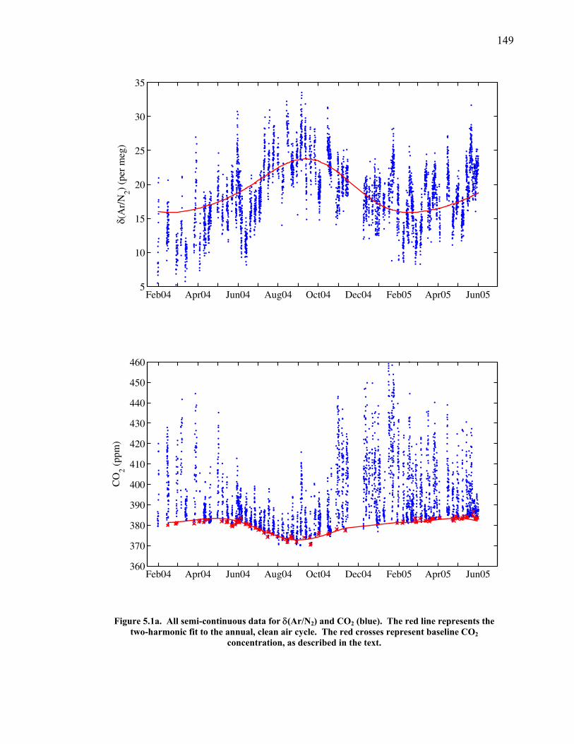
149
δ(A
r/N
2) (p
er m
eg)
Feb04 Apr04 Jun04 Aug04 Oct04 Dec04 Feb05 Apr05 Jun055
10
15
20
25
30
35
CO
2 (pp
m)
Feb04 Apr04 Jun04 Aug04 Oct04 Dec04 Feb05 Apr05 Jun05360
370
380
390
400
410
420
430
440
450
460
Figure 5.1a. All semi-continuous data for δ(Ar/N2) and CO2 (blue). The red line represents the two-harmonic fit to the annual, clean air cycle. The red crosses represent baseline CO2
concentration, as described in the text.
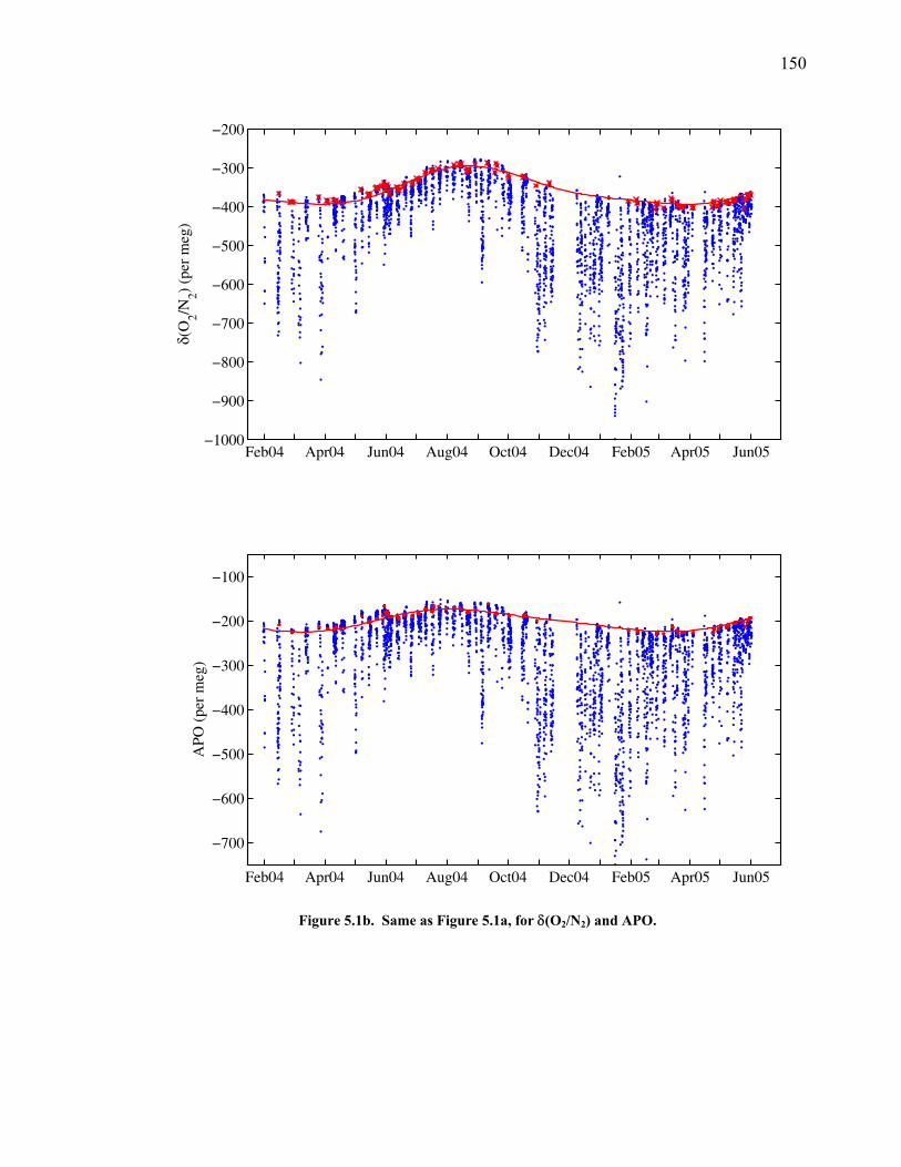
150
δ(O
2/N2)
(per
meg
)
Feb04 Apr04 Jun04 Aug04 Oct04 Dec04 Feb05 Apr05 Jun05−1000
−900
−800
−700
−600
−500
−400
−300
−200
APO
(pe
r m
eg)
Feb04 Apr04 Jun04 Aug04 Oct04 Dec04 Feb05 Apr05 Jun05
−700
−600
−500
−400
−300
−200
−100
Figure 5.1b. Same as Figure 5.1a, for δ(O2/N2) and APO.
151
they should be viewed primarily as deviations from, rather than as part of, the annual
pattern, and therefore two harmonics rather than a larger number were chosen for the
subsequent analysis.
Along with the three species directly measured, atmospheric potential oxygen
(APO) was calculated from the δ(O2/N2) and CO2 concentrations (Figure 5.1b).
Basically, APO is the amount of oxygen left in an air parcel after the CO2 cycle due to
land photosynthesis and respiration has been removed (see Chapter 2 and Stephens et
al. (1998) for a more complete description). APO is conservative to land biology but
reflects the oceanic component in the atmospheric CO2 and δ(O2/N2) cycles. On
seasonal time scales, the oceanic O2 exchange is much larger than the CO2 exchange,
and so APO primarily represents the oceanic component of the δ(O2/N2) cycle.
To extract baseline APO values, it is necessary to derive a baseline CO2
concentration that is uncontaminated with local sources of CO2. The daily CO2
minimum in the hourly record was assumed to be a good “first guess” estimate of
clean air coming off the ocean and uninfluenced by local sources. It was then tested
by looking at the standard deviation around that hourly mean. If the CO2
concentration during the selected hour had a standard deviation above 30 ppm,
showing that the concentration was varying significantly during that time, it was
dropped from the record as representing polluted air derived from over land rather
than clean air derived from over the ocean. If the daily minimum passed this first test,
a second test was conducted that required that the minimum CO2 value lie within an
interval of at least three hours, when the hourly values were all within ±1. Once the
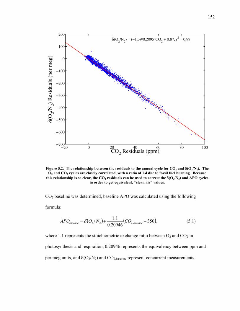
152
CO2 Residuals (ppm)
δ(O
2/N2)
Res
idua
ls (
per
meg
)
δ(O2/N
2) = (−1.39/0.2095)CO
2 + 0.87, r2 = 0.99
−20 0 20 40 60 80 100−700
−600
−500
−400
−300
−200
−100
0
100
200
Figure 5.2. The relationship between the residuals to the annual cycle for CO2 and δ(O2/N2). The O2 and CO2 cycles are closely correlated, with a ratio of 1.4 due to fossil fuel burning. Because
this relationship is so clear, the CO2 residuals can be used to correct the δ(O2/N2) and APO cycles in order to get equivalent, “clean air” values.
CO2 baseline was determined, baseline APO was calculated using the following
formula:
( ) ( )35020946.0
1.1,222 −+= baeslinebaseline CONOAPO δ , (5.1)
where 1.1 represents the stoichiometric exchange ratio between O2 and CO2 in
photosynthesis and respiration, 0.20946 represents the equivalency between ppm and
per meg units, and δ(O2/N2) and CO2,baseline represent concurrent measurements.
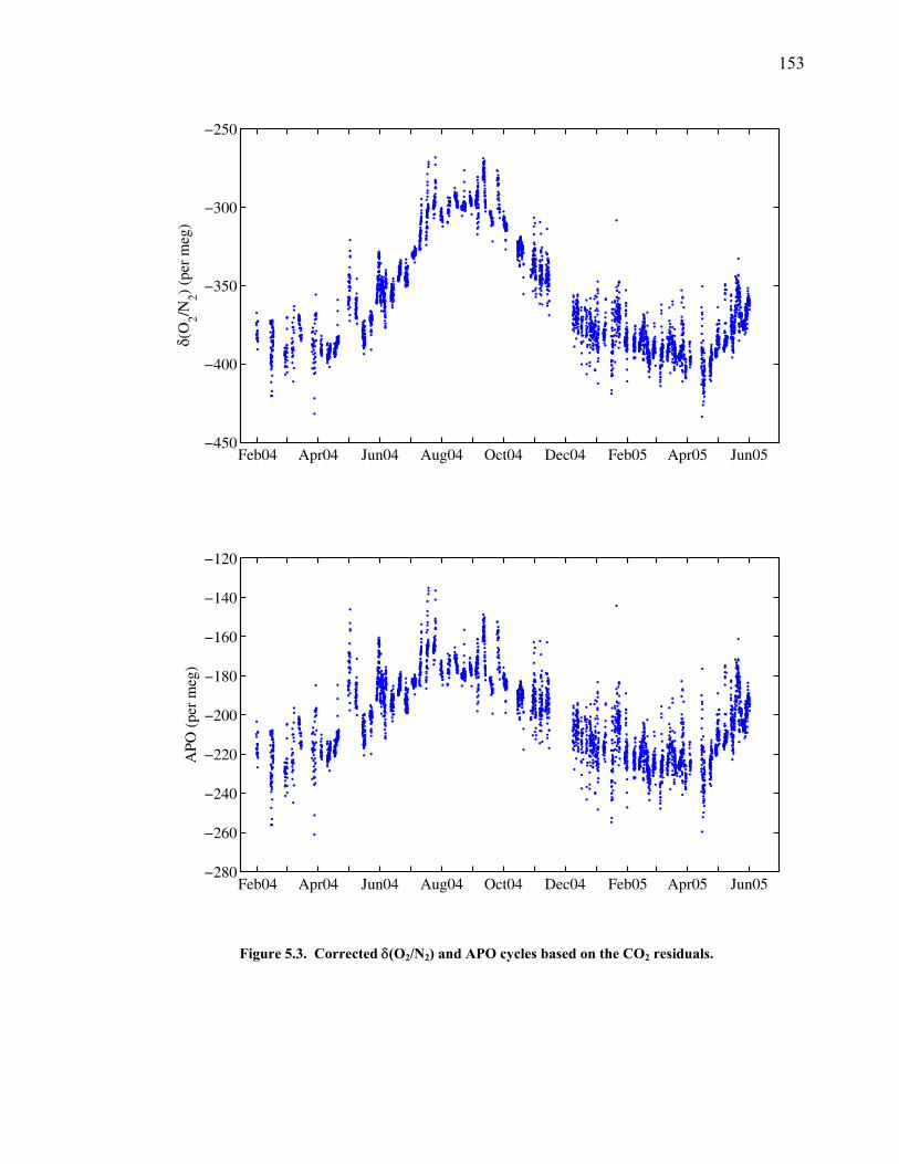
153
δ(O
2/N2)
(per
meg
)
Feb04 Apr04 Jun04 Aug04 Oct04 Dec04 Feb05 Apr05 Jun05−450
−400
−350
−300
−250
APO
(pe
r m
eg)
Feb04 Apr04 Jun04 Aug04 Oct04 Dec04 Feb05 Apr05 Jun05−280
−260
−240
−220
−200
−180
−160
−140
−120
Figure 5.3. Corrected δ(O2/N2) and APO cycles based on the CO2 residuals.
154
Much of the information in the δ(O2/N2) and CO2 records is lost because of the
need to select for clean air conditions. The entire semi-continuous record off of the
Scripps Pier reflects significant land-based pollution from burning of fossil fuels,
which has a different O2:CO2 relationship. A correlation of the deviations of δ(O2/N2)
and CO2 (in per meg equivalent units) from their annual baseline cycles, defined as a
harmonic fit to the points retained in the calculation of APO (above), yield a slope of
-1.39 with an r2 value of 0.99 (see Figure 5.2). Although the local ratio will depend on
the fuel type, this value is very similar to other published values of the O2:CO2 ratio
from burning fossil fuels in Boston (Keeling 1988) and globally (Stephens et al.
1998). I then corrected both the δ(O2/N2) and APO signals for pollution in the entire
record, thus not losing as much information on the synoptic-scale variability in
δ(O2/N2) and APO (see Figure 5.3). In order to do this, I calculated the CO2 residuals
from the annual baseline cycle on an hourly basis. I then used the O2:CO2 ratio of
-1.39 (found above) to calculate the O2-equivalent of these residuals, and I summed
these new terms to the hourly δ(O2/N2) and APO data.
5.3 Seasonal cycles in the data
5.3.1 Seasonal δ(Ar/N2) and its relationship to air-sea heat flux estimates
In mid- to high-latitudes, Ar and N2 are released to the atmosphere in spring
and summer and taken up by the ocean during fall and winter. The maximum in the
seasonal cycle of the La Jolla δ(Ar/N2) data occurs around September 15, whereas the
minimum occurs around February 7. This seasonal pattern is consistent with patterns
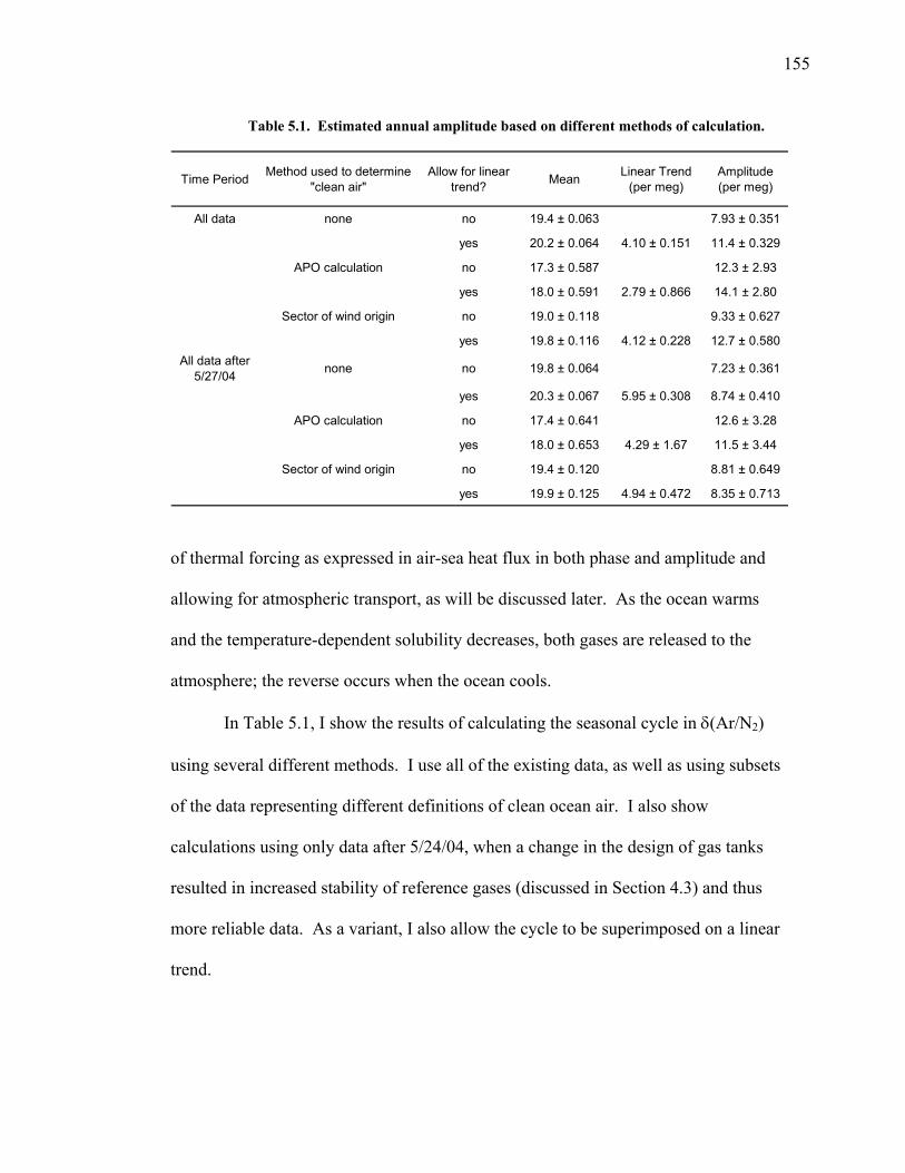
155
Table 5.1. Estimated annual amplitude based on different methods of calculation.
Time Period Method used to determine "clean air"
Allow for linear trend? Mean Linear Trend
(per meg)Amplitude (per meg)
All data none no 19.4 ± 0.063 7.93 ± 0.351
yes 20.2 ± 0.064 4.10 ± 0.151 11.4 ± 0.329
APO calculation no 17.3 ± 0.587 12.3 ± 2.93
yes 18.0 ± 0.591 2.79 ± 0.866 14.1 ± 2.80
Sector of wind origin no 19.0 ± 0.118 9.33 ± 0.627
yes 19.8 ± 0.116 4.12 ± 0.228 12.7 ± 0.580All data after
5/27/04 none no 19.8 ± 0.064 7.23 ± 0.361
yes 20.3 ± 0.067 5.95 ± 0.308 8.74 ± 0.410
APO calculation no 17.4 ± 0.641 12.6 ± 3.28
yes 18.0 ± 0.653 4.29 ± 1.67 11.5 ± 3.44
Sector of wind origin no 19.4 ± 0.120 8.81 ± 0.649
yes 19.9 ± 0.125 4.94 ± 0.472 8.35 ± 0.713
of thermal forcing as expressed in air-sea heat flux in both phase and amplitude and
allowing for atmospheric transport, as will be discussed later. As the ocean warms
and the temperature-dependent solubility decreases, both gases are released to the
atmosphere; the reverse occurs when the ocean cools.
In Table 5.1, I show the results of calculating the seasonal cycle in δ(Ar/N2)
using several different methods. I use all of the existing data, as well as using subsets
of the data representing different definitions of clean ocean air. I also show
calculations using only data after 5/24/04, when a change in the design of gas tanks
resulted in increased stability of reference gases (discussed in Section 4.3) and thus
more reliable data. As a variant, I also allow the cycle to be superimposed on a linear
trend.
156
The annual mean is generally defined statistically to better than 0.2 per meg.
However, the possible presence of a trend renders interpretation of the mean unclear.
The “best-guess” value for the peak-to-peak annual δ(Ar/N2) cycle is most likely
between 8.8 and 9.3 per meg, with an error of about 0.6 per meg. For comparison, the
La Jolla flask measurement record gives a peak-to-peak cycle of 10±3 per meg, using
data from June 2001 to June 2003 (Keeling et al. 2004). In order to calculate this
value, I defined “clean air” for δ(Ar/N2) as those hours in which the air comes from
the sector off the ocean rather than off land (lying between the bearings 225-315o from
due north, as the land is positioned to the west between 350o and 170o) in contrast to
the “clean air” definition used for the calculation of APO. This new definition was
used because the APO definition threw out too many points, resulting in large error
sizes. The APO definition also resulted in an estimate of the amplitude of the annual
δ(Ar/N2) cycle that seemed to be biased low. If all sample hours, clean and polluted
air alike, are used for the estimate of the annual peak-to-peak cycle in δ(Ar/N2), the
estimate is 1-2 per meg smaller. Because pollution visible in the CO2 signal is largest
in the winter when δ(Ar/N2) is smallest, the CO2 correction, as described in Chapter 4,
is largest in the winter as well. If the correction is closer to 12% rather than the
estimated 15%, it is possible that polluted air could cause a bias of 1-2 per meg in the
annual cycle. It is also possible that the wintertime minimum value is biased upward
due to small levels of Ar or N2 pollution in air coming from the land, due to industrial
or laboratory uses.
157
If the seasonal cycle is calculated allowing for a linear trend, it gives a positive
slope of 2.8-5.95 per meg per year (most likely around 4-5 per meg, see Table 5.1).
Adding a linear trend improves the r2 value of the fit (not shown) in every case,
however any determination of a linear trend in 17 months of data is dubious at best.
The modeled increase in heat content of the earth’s oceans is 6.0±0.6 W year m-2
(Hansen et al. 2005), equivalent to an average change in global heat storage of about
1.9x10⁸ J m-2. By comparison, the annual cycle in heat storage is about 7.9 x10⁸ J m-2
for the entire Northern Hemisphere and 8.7 x10⁸ J m-2 for the Southern Hemisphere
(Peixoto and Oort 1992, p. 340). Roughly estimated, these numbers translate into an
annual increase in δ(Ar/N2) of 0.2-0.3 per meg per year. Thus, the observed trend in
δ(Ar/N2) is most likely not due to long-term ocean warming, but instead due to
interannual variability in the air-sea fluxes of Ar and N2 or unresolved sampling or
calibration problems. Keeling et al. (2004) suggest that the interannual variability
should be on the order of ±1-2 per meg per year, based on estimates of variability in
heat storage. Significant interannual variability has already been noted in model
predictions and measurements of air-sea fluxes of oxygen: Bopp et al. (2002) project
variability on the order of 20% of the average annual emissions of tropical oceans;
McKinley et al. (2003) estimate 35-50%, and McKinley et al. (2000) suggests a value
of about 40% of the mean flux in the North Atlantic. Garcia et al. (2005) have shown
interannual variability of about 25% in comparison to the seasonal cycle of the
Northern Hemisphere ocean oxygen content. This variability, caused by changes in
ocean stratification, is likely to impact air-sea Ar and N2 fluxes as well.
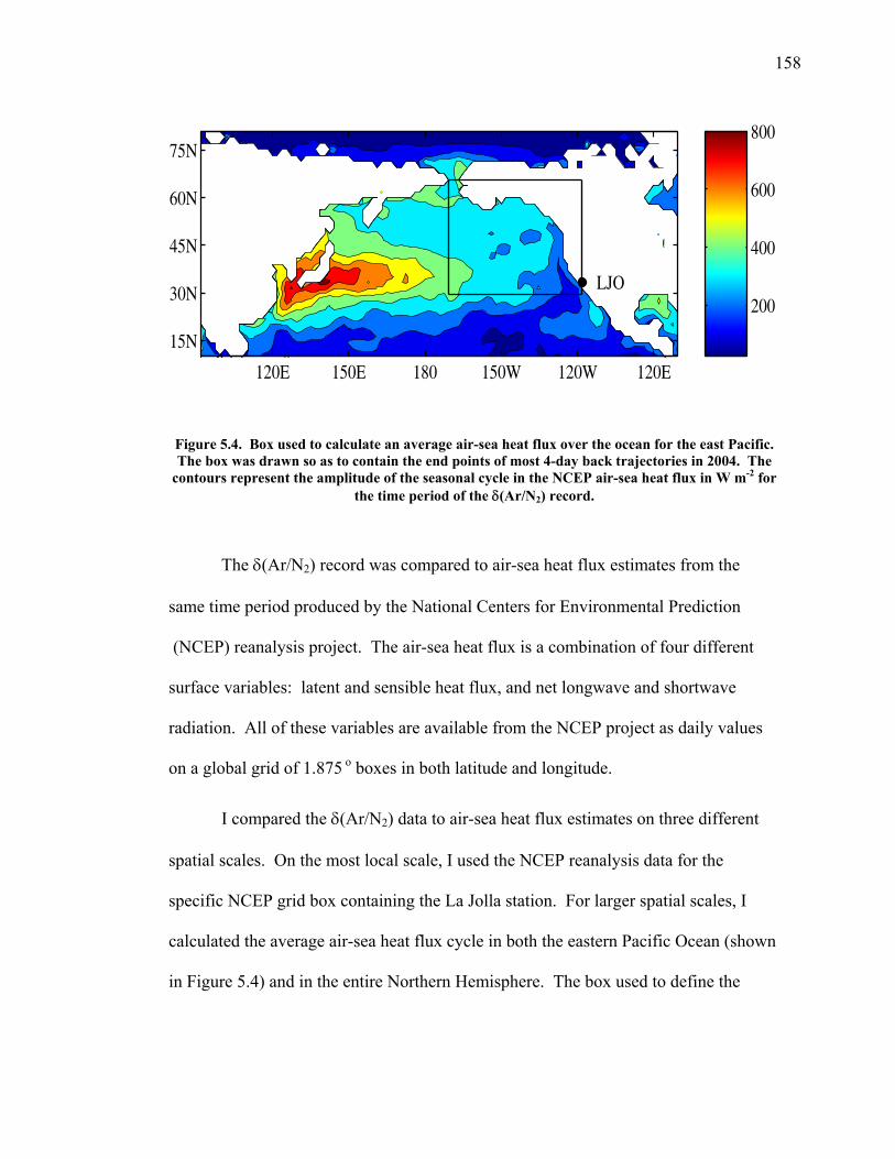
158
LJO
120E 150E 180 150W 120W 120E
15N
30N
45N
60N
75N
200
400
600
800
Figure 5.4. Box used to calculate an average air-sea heat flux over the ocean for the east Pacific. The box was drawn so as to contain the end points of most 4-day back trajectories in 2004. The
contours represent the amplitude of the seasonal cycle in the NCEP air-sea heat flux in W m-2 for the time period of the δ(Ar/N2) record.
The δ(Ar/N2) record was compared to air-sea heat flux estimates from the
same time period produced by the National Centers for Environmental Prediction
(NCEP) reanalysis project. The air-sea heat flux is a combination of four different
surface variables: latent and sensible heat flux, and net longwave and shortwave
radiation. All of these variables are available from the NCEP project as daily values
on a global grid of 1.875 o boxes in both latitude and longitude.
I compared the δ(Ar/N2) data to air-sea heat flux estimates on three different
spatial scales. On the most local scale, I used the NCEP reanalysis data for the
specific NCEP grid box containing the La Jolla station. For larger spatial scales, I
calculated the average air-sea heat flux cycle in both the eastern Pacific Ocean (shown
in Figure 5.4) and in the entire Northern Hemisphere. The box used to define the
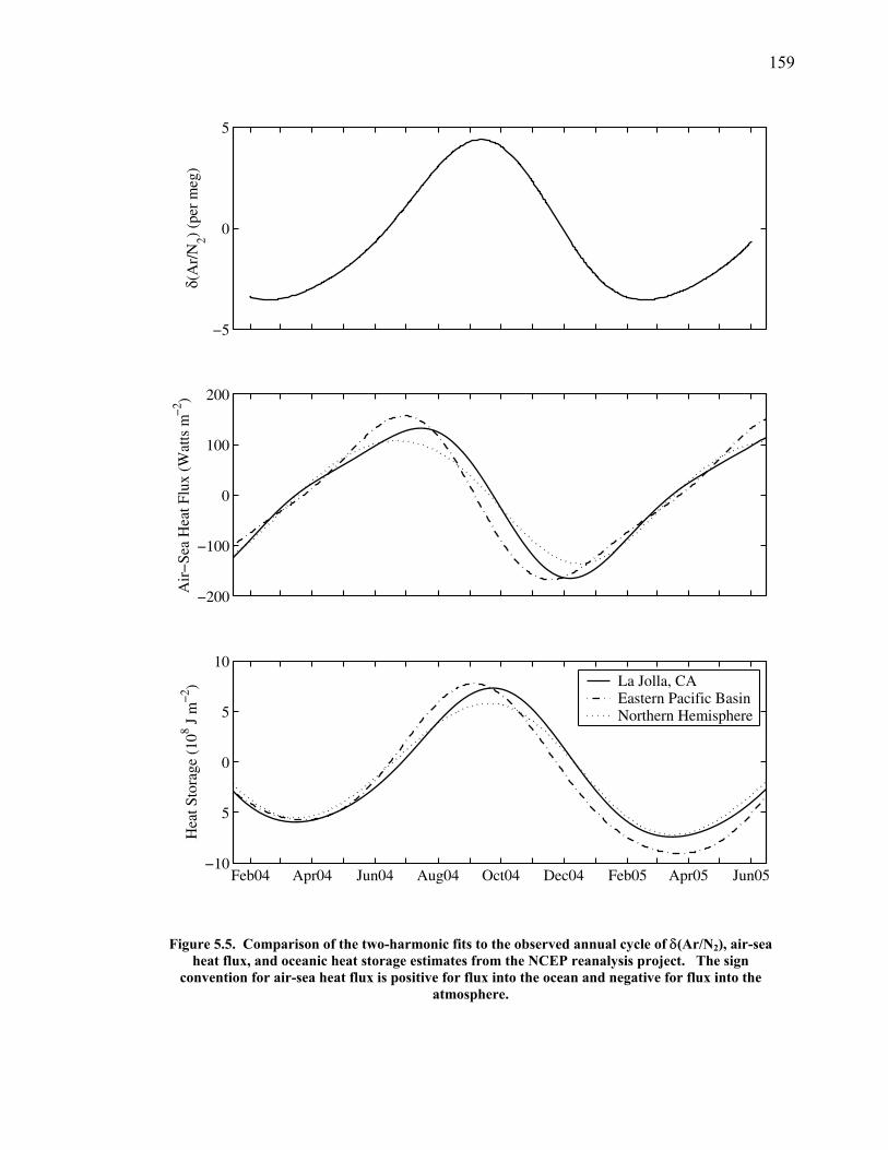
159
δ(A
r/N
2) (p
er m
eg)
−5
0
5
Air−
Sea
Hea
t Flu
x (W
atts
m−
2 )
−200
−100
0
100
200
Hea
t Sto
rage
(10
8 J m
−2 )
Feb04 Apr04 Jun04 Aug04 Oct04 Dec04 Feb05 Apr05 Jun05−10
5
0
5
10La Jolla, CAEastern Pacific BasinNorthern Hemisphere
Figure 5.5. Comparison of the two-harmonic fits to the observed annual cycle of δ(Ar/N2), air-sea heat flux, and oceanic heat storage estimates from the NCEP reanalysis project. The sign
convention for air-sea heat flux is positive for flux into the ocean and negative for flux into the atmosphere.
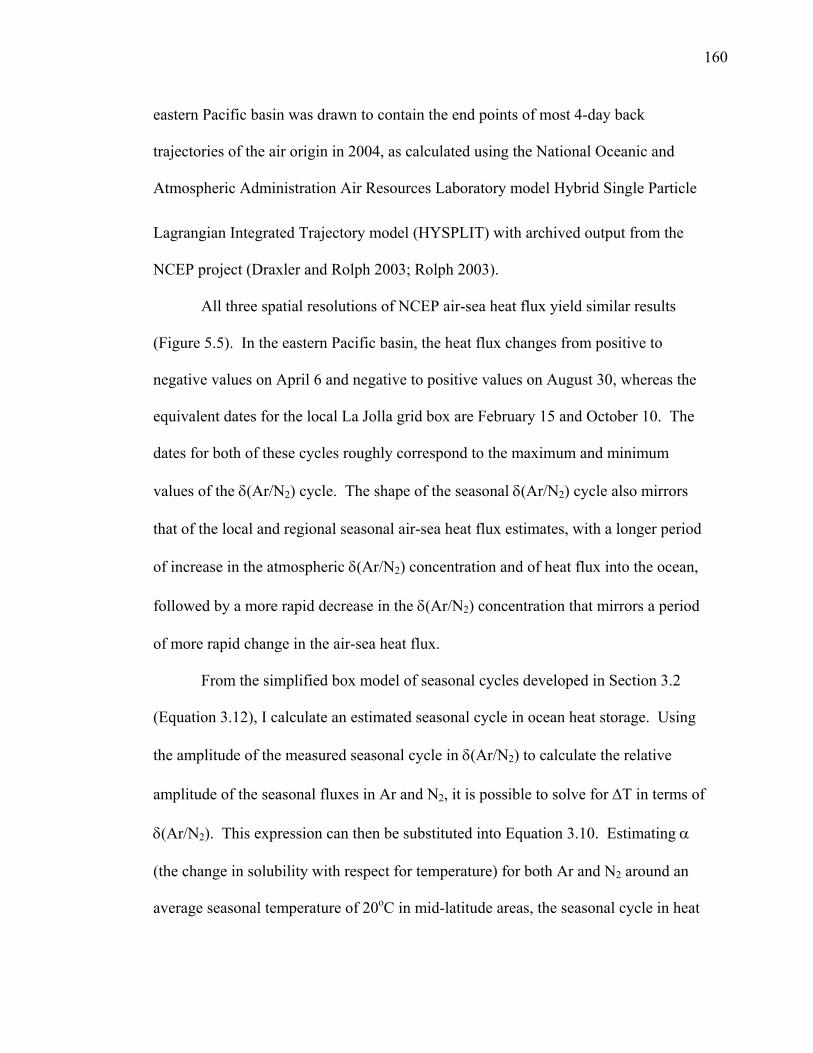
160
eastern Pacific basin was drawn to contain the end points of most 4-day back
trajectories of the air origin in 2004, as calculated using the National Oceanic and
Atmospheric Administration Air Resources Laboratory model Hybrid Single Particle
Lagrangian Integrated Trajectory model (HYSPLIT) with archived output from the
NCEP project (Draxler and Rolph 2003; Rolph 2003).
All three spatial resolutions of NCEP air-sea heat flux yield similar results
(Figure 5.5). In the eastern Pacific basin, the heat flux changes from positive to
negative values on April 6 and negative to positive values on August 30, whereas the
equivalent dates for the local La Jolla grid box are February 15 and October 10. The
dates for both of these cycles roughly correspond to the maximum and minimum
values of the δ(Ar/N2) cycle. The shape of the seasonal δ(Ar/N2) cycle also mirrors
that of the local and regional seasonal air-sea heat flux estimates, with a longer period
of increase in the atmospheric δ(Ar/N2) concentration and of heat flux into the ocean,
followed by a more rapid decrease in the δ(Ar/N2) concentration that mirrors a period
of more rapid change in the air-sea heat flux.
From the simplified box model of seasonal cycles developed in Section 3.2
(Equation 3.12), I calculate an estimated seasonal cycle in ocean heat storage. Using
the amplitude of the measured seasonal cycle in δ(Ar/N2) to calculate the relative
amplitude of the seasonal fluxes in Ar and N2, it is possible to solve for ΔT in terms of
δ(Ar/N2). This expression can then be substituted into Equation 3.10. Estimating α
(the change in solubility with respect for temperature) for both Ar and N2 around an
average seasonal temperature of 20oC in mid-latitude areas, the seasonal cycle in heat
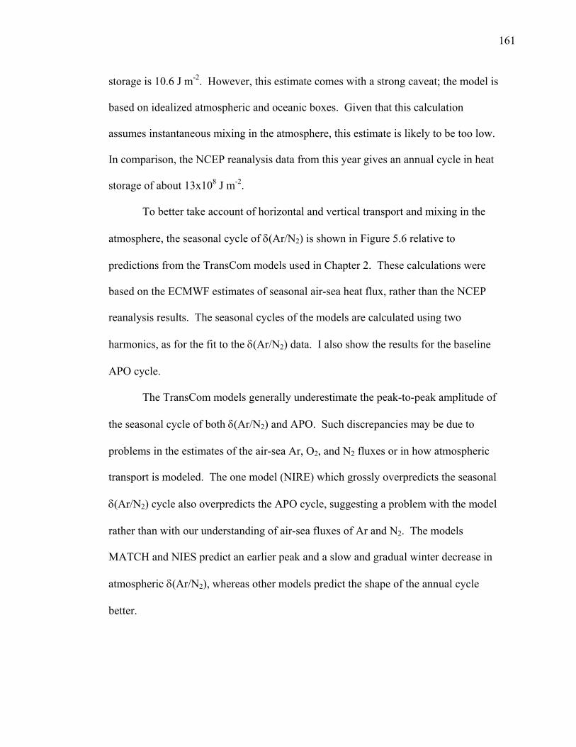
161
storage is 10.6 J m-2. However, this estimate comes with a strong caveat; the model is
based on idealized atmospheric and oceanic boxes. Given that this calculation
assumes instantaneous mixing in the atmosphere, this estimate is likely to be too low.
In comparison, the NCEP reanalysis data from this year gives an annual cycle in heat
storage of about 13x108 J m-2.
To better take account of horizontal and vertical transport and mixing in the
atmosphere, the seasonal cycle of δ(Ar/N2) is shown in Figure 5.6 relative to
predictions from the TransCom models used in Chapter 2. These calculations were
based on the ECMWF estimates of seasonal air-sea heat flux, rather than the NCEP
reanalysis results. The seasonal cycles of the models are calculated using two
harmonics, as for the fit to the δ(Ar/N2) data. I also show the results for the baseline
APO cycle.
The TransCom models generally underestimate the peak-to-peak amplitude of
the seasonal cycle of both δ(Ar/N2) and APO. Such discrepancies may be due to
problems in the estimates of the air-sea Ar, O2, and N2 fluxes or in how atmospheric
transport is modeled. The one model (NIRE) which grossly overpredicts the seasonal
δ(Ar/N2) cycle also overpredicts the APO cycle, suggesting a problem with the model
rather than with our understanding of air-sea fluxes of Ar and N2. The models
MATCH and NIES predict an earlier peak and a slow and gradual winter decrease in
atmospheric δ(Ar/N2), whereas other models predict the shape of the annual cycle
better.
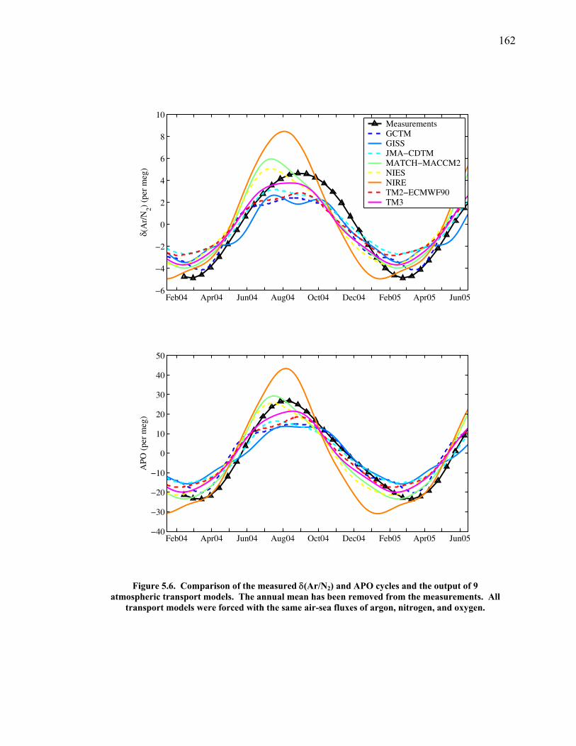
162
δ(A
r/N
2) (p
er m
eg)
Feb04 Apr04 Jun04 Aug04 Oct04 Dec04 Feb05 Apr05 Jun05−6
−4
−2
0
2
4
6
8
10MeasurementsGCTMGISSJMA−CDTMMATCH−MACCM2NIESNIRETM2−ECMWF90TM3
APO
(pe
r m
eg)
Feb04 Apr04 Jun04 Aug04 Oct04 Dec04 Feb05 Apr05 Jun05−40
−30
−20
−10
0
10
20
30
40
50
Figure 5.6. Comparison of the measured δ(Ar/N2) and APO cycles and the output of 9 atmospheric transport models. The annual mean has been removed from the measurements. All
transport models were forced with the same air-sea fluxes of argon, nitrogen, and oxygen.
163
This model/data discrepancy may be due to the wind fields chosen to drive
specific atmospheric transport models. It suggests that we may also expect to see such
variability in the shape of the seasonal cycle on interannual time scales. The annual
maximum and its timing may also be problematic in many models due to seasonal
changes in atmospheric transport that are not accurately described. In 2004, for
example, the wind speed tended to be low through the summer months. Although the
wind speed began increasing again in September, it dropped again in October, a
phenomenon that models may not be able to accurately capture. The measured annual
cycle may have been affected by weaker vertical mixing in the atmosphere throughout
the summertime in comparison to other times, leading to a higher maximum than
generally expected. However, differences between predictions and measurements may
also be a more systematic problem related to the difficulty of modeling the
complexities of atmospheric transport near the La Jolla station. Most likely, the
models fail to accurately describe the low-level coastal jets which form above the
marine boundary layer, especially during the summer (Burk and Thompson 1996). La
Jolla may be receiving more air with a northern origin (and a larger expected seasonal
cycle in Ar/N2) than the models are able to predict.
5.3.2 Seasonal cycles of CO2, δ(O2/N2) and APO
The peak-to-peak amplitude of the measured clean-air seasonal cycles in the
semi-continuous measurements, based on a 2-harmonic fit, are 10.80 ppm in CO2,
98.69 per meg in δ(O2/N2), and 50.86 per meg in APO (Figure 5.1). These numbers
164
compare quite closely to the cycles of 10.39 ppm, 103.74 per meg, and 53.99 per meg
measured in Scripps Institution of Oceanography flask sampling program since 1989
(described in Chapter 4; Keeling et al. 1998). These numbers provide an important
check on the continuous measurement system, showing that any systematic sampling
problems are smaller than that which can be generally detected in the δ(O2/N2) or CO2
cycles. They also validate the criterion used for sampling clean air in the flask
measurement program.
In parallel with the δ(Ar/N2) cycle, discussed above, Keeling et al. (1998)
observe that atmospheric transport models tend to underestimate the APO cycle at La
Jolla, as they do the δ(Ar/N2) cycle. They hypothesize that there is a discrepancy
between the modeled seasonal cycle and the observed one because technicians actively
select for steady, west-wind conditions in order to minimize pollution, whereas the
model results do not reflect specific wind conditions. Because the data workup selects
for clean air times in the sampling record in a similar way to that in which a technician
selects for clean air in the flask sampling program, the semi-continuous measurements
will likely have a similar bias towards air masses with an origin over the ocean.
However, the corrected data shown in Figure 5.3, which are not selected for specific
wind conditions, yield an annual amplitude of 98.79 per meg for δ(O2/N2) and 50.86
per meg for APO. The difference in predictions for the δ(Ar/N2) cycle between the
best “clean air” estimates and estimates using all data is in the range of 1-2 per meg as
well. This observation suggests that the “clean air” cycles are probably not
significantly biased by the origin of selected air, in contrast to the explanation in
165
Keeling et al. (1998), and implies that the discrepancy between models and predictions
lie with problems in the models.
5.3.3 Components of the seasonal cycle of δ(O2/N2)
Based on the solubility of O2, Ar, and N2 in seawater (Weiss 1970), the
expected atmospheric δ(O2/N2):δ(Ar/N2) ratio due to seawater warming and cooling
ranges from 0.83 at 25oC to 0.85 at 0oC. Keeling and Garcia (2002) suggest that the
actual relationship between air-sea heat flux and O2 flux may be very different from
the expected relationship based on heat flux alone; the effects of biological production
and respiration and seasonal changes in the ocean structure can be several times larger
than the effects of air-sea heat flux on the oxygen cycle. They calculate an estimated
oxygen flux per joule of heat flux of 5 nmol J-1 in mid-latitudes on seasonal time
scales (Keeling and Garcia 2002), with model results predicting 6 nmol J-1 (Sarmiento
et al. 1998, as quoted in Bopp et al. 2002) and 6.1 nmol J-1 (Bopp et al. 2002).
Atmospheric transport model results based on satellite estimates of ocean primary
production suggest that 88% of the seasonal δ(O2/N2) cycle at the La Jolla station is
due to marine biology and ventilation, while changes in solubility account for only
12% (Balkanski et al. 1999), giving a ratio around 7. Keeling and Garcia (2002)
suggest an O2 flux/heating ratio of about 5 nmol J-1 for mid-latitudes, based on
measurements of ocean oxygen concentrations. Using the estimated relationship
between δ(Ar/N2) and δ(O2/N2) due to differences in solubility, this value is equivalent
to an expected ratio of 3.5 for atmospheric APO:δ(Ar/N2), given an average surface
166
water temperature of 15-20oC in mid-latitudes. APO is used rather than δ(O2/N2)
because APO represents the oceanic component of the atmospheric δ(O2/N2) signal.
Comparison of the size of the annual cycles in the continuous measurements
results in a ratio of APO to δ(Ar/N2) of 5.5, which fits in with the above estimates.
The maximum of the seasonal ocean heat storage cycle in September 2004 minus the
minimum in March 2005 gives a cycle on the order of 14.7x10⁸ J m-2 in La Jolla and
16.8x10⁸ J m-2 in the eastern Pacific basin, compared to the long-term average of
13.7x10⁸ J m-2 in La Jolla and 13.1x10⁸ J m-2 in the eastern Pacific basin from 1950-
2004. The comparison suggests that the heat component of the APO cycle during the
2004-2005 period in which there are semi-continuous measurements may be larger
than the average, reducing the ratio between APO and δ(Ar/N2). Although ocean
biology would presumably change in response to the dynamical effects of a larger
ocean heat storage cycle, it may not be able to respond as fast or as completely as
solubility-driven changes in the air-sea gas fluxes.
Parallel measurements of CO2, APO, and δ(Ar/N2) make it possible to piece
out what part of the δ(O2/N2) cycle is due to land biology (the difference between
δ(O2/N2) and APO), air-sea heat flux (the δ(Ar/N2) cycle times the expected
atmospheric δ(O2/N2):δ(Ar/N2) ratio of 0.84 derived from differences in solubility in
Weiss 1970), and ocean structural and biological changes (the remainder). All three of
these cycles, shown in Figure 5.7, have distinct amplitudes and timing. Garcia and
Keeling (2001) conclude that the peak of the O2 cycle due to ocean stratification and
biology is closely correlated with the peak of the timing of the air-sea heat flux. More
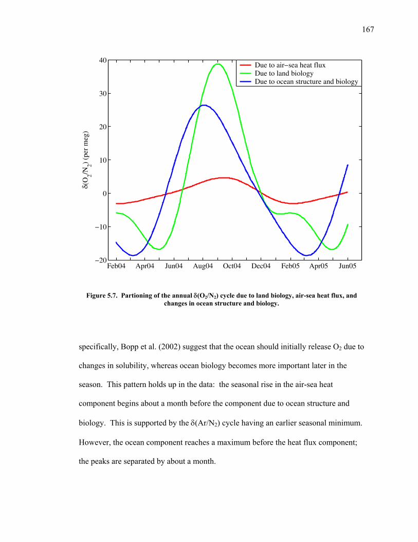
167
δ(O
2/N2)
(per
meg
)
Feb04 Apr04 Jun04 Aug04 Oct04 Dec04 Feb05 Apr05 Jun05−20
−10
0
10
20
30
40Due to air−sea heat fluxDue to land biologyDue to ocean structure and biology
Figure 5.7. Partioning of the annual δ(O2/N2) cycle due to land biology, air-sea heat flux, and changes in ocean structure and biology.
specifically, Bopp et al. (2002) suggest that the ocean should initially release O2 due to
changes in solubility, whereas ocean biology becomes more important later in the
season. This pattern holds up in the data: the seasonal rise in the air-sea heat
component begins about a month before the component due to ocean structure and
biology. This is supported by the δ(Ar/N2) cycle having an earlier seasonal minimum.
However, the ocean component reaches a maximum before the heat flux component;
the peaks are separated by about a month.
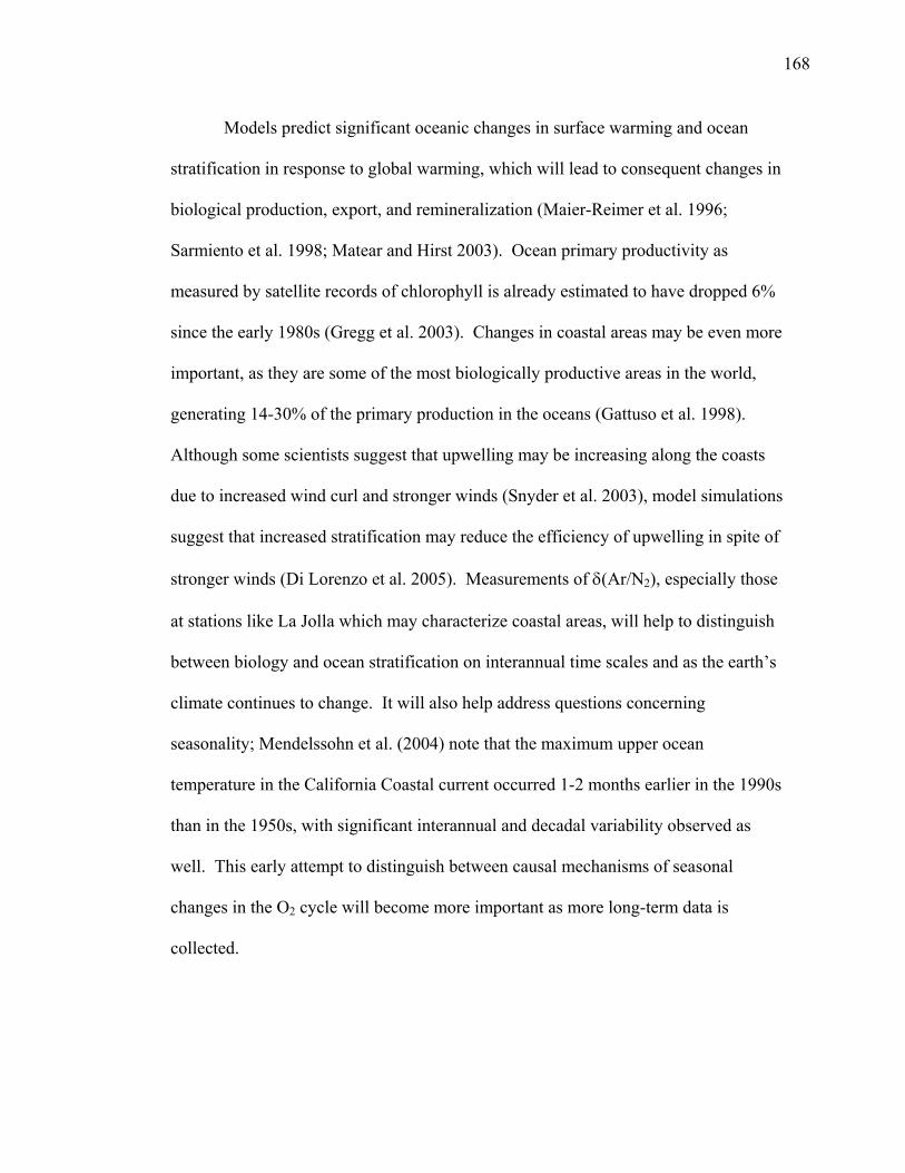
168
Models predict significant oceanic changes in surface warming and ocean
stratification in response to global warming, which will lead to consequent changes in
biological production, export, and remineralization (Maier-Reimer et al. 1996;
Sarmiento et al. 1998; Matear and Hirst 2003). Ocean primary productivity as
measured by satellite records of chlorophyll is already estimated to have dropped 6%
since the early 1980s (Gregg et al. 2003). Changes in coastal areas may be even more
important, as they are some of the most biologically productive areas in the world,
generating 14-30% of the primary production in the oceans (Gattuso et al. 1998).
Although some scientists suggest that upwelling may be increasing along the coasts
due to increased wind curl and stronger winds (Snyder et al. 2003), model simulations
suggest that increased stratification may reduce the efficiency of upwelling in spite of
stronger winds (Di Lorenzo et al. 2005). Measurements of δ(Ar/N2), especially those
at stations like La Jolla which may characterize coastal areas, will help to distinguish
between biology and ocean stratification on interannual time scales and as the earth’s
climate continues to change. It will also help address questions concerning
seasonality; Mendelssohn et al. (2004) note that the maximum upper ocean
temperature in the California Coastal current occurred 1-2 months earlier in the 1990s
than in the 1950s, with significant interannual and decadal variability observed as
well. This early attempt to distinguish between causal mechanisms of seasonal
changes in the O2 cycle will become more important as more long-term data is
collected.
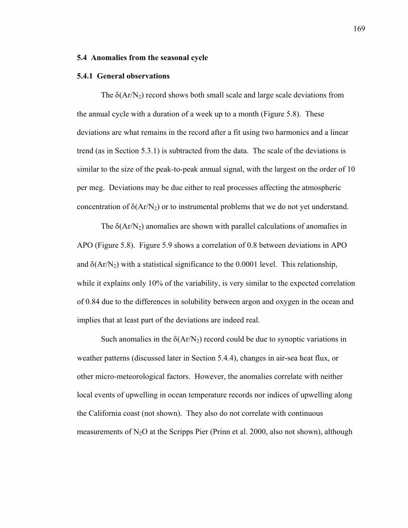
169
5.4 Anomalies from the seasonal cycle
5.4.1 General observations
The δ(Ar/N2) record shows both small scale and large scale deviations from
the annual cycle with a duration of a week up to a month (Figure 5.8). These
deviations are what remains in the record after a fit using two harmonics and a linear
trend (as in Section 5.3.1) is subtracted from the data. The scale of the deviations is
similar to the size of the peak-to-peak annual signal, with the largest on the order of 10
per meg. Deviations may be due either to real processes affecting the atmospheric
concentration of δ(Ar/N2) or to instrumental problems that we do not yet understand.
The δ(Ar/N2) anomalies are shown with parallel calculations of anomalies in
APO (Figure 5.8). Figure 5.9 shows a correlation of 0.8 between deviations in APO
and δ(Ar/N2) with a statistical significance to the 0.0001 level. This relationship,
while it explains only 10% of the variability, is very similar to the expected correlation
of 0.84 due to the differences in solubility between argon and oxygen in the ocean and
implies that at least part of the deviations are indeed real.
Such anomalies in the δ(Ar/N2) record could be due to synoptic variations in
weather patterns (discussed later in Section 5.4.4), changes in air-sea heat flux, or
other micro-meteorological factors. However, the anomalies correlate with neither
local events of upwelling in ocean temperature records nor indices of upwelling along
the California coast (not shown). They also do not correlate with continuous
measurements of N2O at the Scripps Pier (Prinn et al. 2000, also not shown), although
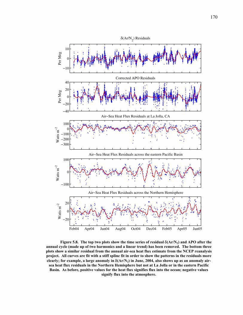
170
δ(Ar/N2) Residuals
Per
Meg
−10
0
10
Corrected APO Residuals
Per
Meg
−40
−20
0
20
40
Air−Sea Heat Flux Residuals at La Jolla, CA
Wat
ts m
−2
−300−200−100
0100
Air−Sea Heat Flux Residuals across the eastern Pacific Basin
Wat
ts m
−2
−100
0
100
Air−Sea Heat Flux Residuals across the Northern Hemisphere
Wat
ts m
−2
Feb04 Apr04 Jun04 Aug04 Oct04 Dec04 Feb05 Apr05 Jun05
−20
0
20
Figure 5.8. The top two plots show the time series of residual δ(Ar/N2) and APO after the
annual cycle (made up of two harmonics and a linear trend) has been removed. The bottom three plots show a similar residual from the annual air-sea heat flux estimate from the NCEP reanalysis project. All curves are fit with a stiff spline fit in order to show the patterns in the residuals more clearly; for example, a large anomaly in δ(Ar/N2) in June, 2004, also shows up as an anomaly air-
sea heat flux residuals in the Northern Hemisphere but not at La Jolla or in the eastern Pacific Basin. As before, positive values for the heat flux signifies flux into the ocean; negative values
signify flux into the atmosphere.
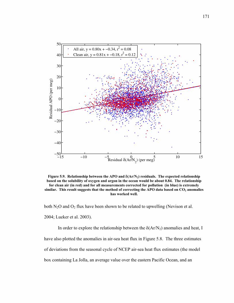
171
Res
idua
l APO
(pe
r m
eg)
Residual δ(Ar/N2) (per meg)
−15 −10 −5 0 5 10 15−50
−40
−30
−20
−10
0
10
20
30
40
50All air, y = 0.80x + −0.34, r2 = 0.08Clean air, y = 0.81x + −0.18, r2 = 0.12
Figure 5.9. Relationship between the APO and δ(Ar/N2) residuals. The expected relationship based on the solubility of oxygen and argon in the ocean would be about 0.84. The relationship
for clean air (in red) and for all measurements corrected for pollution (in blue) is extremely similar. This result suggests that the method of correcting the APO data based on CO2 anomalies
has worked well.
both N2O and O2 flux have been shown to be related to upwelling (Nevison et al.
2004; Lueker et al. 2003).
In order to explore the relationship between the δ(Ar/N2) anomalies and heat, I
have also plotted the anomalies in air-sea heat flux in Figure 5.8. The three estimates
of deviations from the seasonal cycle of NCEP air-sea heat flux estimates (the model
box containing La Jolla, an average value over the eastern Pacific Ocean, and an
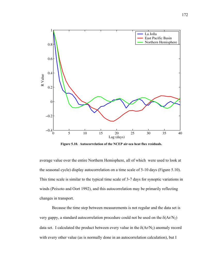
172
Lag (days)
R V
alue
0 5 10 15 20 25 30 35 40−0.4
−0.2
0
0.2
0.4
0.6
0.8
1La JollaEast Pacific BasinNorthern Hemisphere
Figure 5.10. Autocorrelation of the NCEP air-sea heat flux residuals.
average value over the entire Northern Hemisphere, all of which were used to look at
the seasonal cycle) display autocorrelation on a time scale of 5-10 days (Figure 5.10).
This time scale is similar to the typical time scale of 3-7 days for synoptic variations in
winds (Peixoto and Oort 1992), and this autocorrelation may be primarily reflecting
changes in transport.
Because the time step between measurements is not regular and the data set is
very gappy, a standard autocorrelation procedure could not be used on the δ(Ar/N2)
data set. I calculated the product between every value in the δ(Ar/N2) anomaly record
with every other value (as is normally done in an autocorrelation calculation), but I
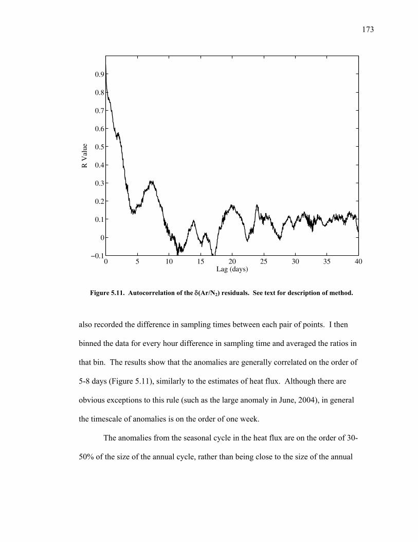
173
R V
alue
Lag (days)0 5 10 15 20 25 30 35 40
−0.1
0
0.1
0.2
0.3
0.4
0.5
0.6
0.7
0.8
0.9
Figure 5.11. Autocorrelation of the δ(Ar/N2) residuals. See text for description of method.
also recorded the difference in sampling times between each pair of points. I then
binned the data for every hour difference in sampling time and averaged the ratios in
that bin. The results show that the anomalies are generally correlated on the order of
5-8 days (Figure 5.11), similarly to the estimates of heat flux. Although there are
obvious exceptions to this rule (such as the large anomaly in June, 2004), in general
the timescale of anomalies is on the order of one week.
The anomalies from the seasonal cycle in the heat flux are on the order of 30-
50% of the size of the annual cycle, rather than being close to the size of the annual
174
signal itself. Although certain peaks in the residuals of the heat flux seem related to
peaks in the δ(Ar/N2) residuals, a statistical comparison of three different estimates for
air sea heat flux using the NCEP reanalysis output used for the annual cycle shows
that only the La Jolla estimate has any correlation to the variation in δ(Ar/N2),
accounting for less than 5% of the variability. The other two estimates show no
correlation between δ(Ar/N2) and large-scale air-sea heat flux anomaly estimates at
all. Comparing NCEP reanalysis output from 1950-2003 with the 2004-2005
anomalies in the δ(Ar/N2) record actually suggests that previous years’ air-sea heat
flux estimates sometime correlate better than the 2004-2005 NCEP reanalysis output,
thus supporting the conclusion that there is no real correlation.
Although comparison with the anomalies in the NCEP reanalysis output does
not suggest a link between deviations in the δ(Ar/N2) cycle and deviations from the
seasonal cycle of large-scale estimates of air-sea heat flux, it is also possible to look at
local weather variables for evidence of changes in air-sea heat flux. The weather
station on the pier collects information on atmospheric and oceanic variables every
five minutes. I then averaged the data into hourly values, more appropriate for
comparison with the δ(Ar/N2) data, and removed the seasonal cycle. Key variables
likely to be correlated with δ(Ar/N2) include ocean water temperature and air
temperature, both linked to air-sea heat flux. Other likely candidates include wind
speed, wind direction, photosynthetically active radiation (PAR), and barometric
pressure as weather systems move through the area. However, both on time scales of
an hour and of a day, there are either no or extremely weak correlations. Wind speed,
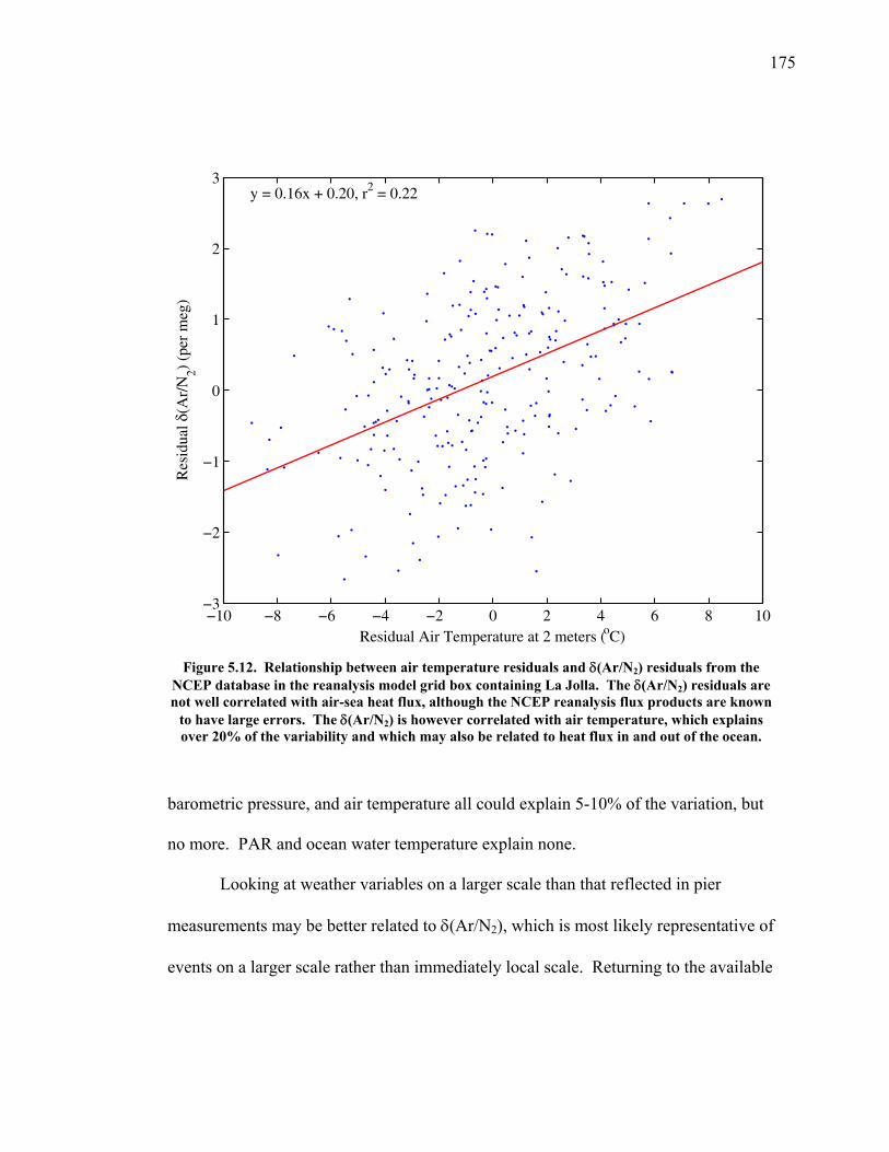
175
Residual Air Temperature at 2 meters (oC)
Res
idua
l δ(A
r/N
2) (p
er m
eg)
y = 0.16x + 0.20, r2 = 0.22
−10 −8 −6 −4 −2 0 2 4 6 8 10−3
−2
−1
0
1
2
3
Figure 5.12. Relationship between air temperature residuals and δ(Ar/N2) residuals from the
NCEP database in the reanalysis model grid box containing La Jolla. The δ(Ar/N2) residuals are not well correlated with air-sea heat flux, although the NCEP reanalysis flux products are known
to have large errors. The δ(Ar/N2) is however correlated with air temperature, which explains over 20% of the variability and which may also be related to heat flux in and out of the ocean.
barometric pressure, and air temperature all could explain 5-10% of the variation, but
no more. PAR and ocean water temperature explain none.
Looking at weather variables on a larger scale than that reflected in pier
measurements may be better related to δ(Ar/N2), which is most likely representative of
events on a larger scale rather than immediately local scale. Returning to the available
176
NCEP reanalysis output, daily deviations in estimated air temperature from the
seasonal cycle at 2 meters above the surface in the model box containing La Jolla
explain about 20% of daily δ(Ar/N2) deviations (Figure 5.12), which could arguably
be tied to air-sea heat flux. A similar correlation is weaker for other variables
available from the NCEP dataset, such as surface air pressure and wind direction.
An analysis of the power spectrum from seven of the longest gap-free periods with at
least three days of data does not show any suggestion of a periodic processes related to
the anomalies. Instead, it suggests that any pattern on timescales of less than a month
may be attributable to transport of a passive marker in a turbulent system. However,
this analysis also isolates three periods with a different pattern, suggesting that the
assumption of a stationary stochastic process is not strong, and different mechanisms
may be causing the anomalies in different periods (R. L. Parker, personal
communication). The first of these periods will be discussed next; the other two fall
into the period from 12/1/04-6/1/05.
5.4.2 June 2004 anomaly
The anomaly in June, 2004, is the largest so far in the record. It persists for a
month, rising initially to 10 per meg over the seasonal cycle and then dropping in
about a week to 10 per meg below the cycle, slowly rebounding over the next few
weeks. A comparison of the anomalies in δ(Ar/N2) and heat flux estimates in Figure
5.8 also shows that the largest negative anomaly in heat flux in the Northern
Hemisphere average occurs at the same time, showing up (but not as strongly) in the
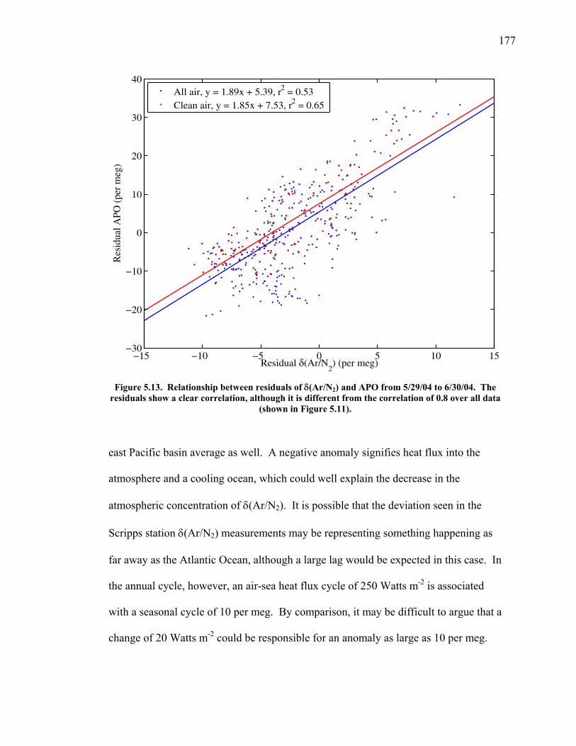
177
Res
idua
l APO
(pe
r m
eg)
Residual δ(Ar/N2) (per meg)
−15 −10 −5 0 5 10 15−30
−20
−10
0
10
20
30
40All air, y = 1.89x + 5.39, r2 = 0.53Clean air, y = 1.85x + 7.53, r2 = 0.65
Figure 5.13. Relationship between residuals of δ(Ar/N2) and APO from 5/29/04 to 6/30/04. The
residuals show a clear correlation, although it is different from the correlation of 0.8 over all data (shown in Figure 5.11).
east Pacific basin average as well. A negative anomaly signifies heat flux into the
atmosphere and a cooling ocean, which could well explain the decrease in the
atmospheric concentration of δ(Ar/N2). It is possible that the deviation seen in the
Scripps station δ(Ar/N2) measurements may be representing something happening as
far away as the Atlantic Ocean, although a large lag would be expected in this case. In
the annual cycle, however, an air-sea heat flux cycle of 250 Watts m-2 is associated
with a seasonal cycle of 10 per meg. By comparison, it may be difficult to argue that a
change of 20 Watts m-2 could be responsible for an anomaly as large as 10 per meg.
178
However, it is feasible that a short-term anomaly would not mix as far into the
atmosphere and would result in anomalous δ(Ar/N2) concentrations as measured at the
sea surface level.
During this period, the ratio between APO and δ(Ar/N2) anomalies differs
from the ratio of 0.8 common over the entire record; instead, it is closer to 1.8-1.9, and
the ratio accounts for 50-65% of the relationship between the two variables, a much
larger percentage (Figure 5.13). Thermal fractionation would imply a ratio close to
0.25; although it may not be possible to dismiss the possibility that instrumental
problems are the cause of the change in the ratio, this anomaly seems to be real and
not just a measurement problem.
This anomaly occurs at the same time as the cloudiest month on record since
the beginning of the semi-continuous δ(Ar/N2) measurements. During this period, the
anomaly record of air temperature is close to zero and has little variability compared
to the overall record of anomalies. Wind speed anomalies are also small. Although
upwelling events occur over the months of May and June, with a large event lasting
from 5/30/04 to 6/6/04, a larger and more sustained upwelling event occurs in mid- to
late-July when the δ(Ar/N2) concentration is more stable. However, the δ(Ar/N2)
anomaly is loosely correlated with changes in the record of photosynthetically active
radiation (PAR, a measure of incoming solar radiation that falls between 400-700 nm)
as measured by the weather station on the Scripps pier. It is possible, though
speculative, that the change in PAR represents short-term, localized changes in air-sea
heat flux that could result in a sudden change in atmospheric δ(Ar/N2). An increase in
179
PAR most likely represents heat flux into the ocean, and thus atmospheric δ(Ar/N2)
values would be expected to increase as well. These results suggest that localized
events (such as the strongly stratified marine boundary layer common off the coast of
La Jolla in June) can have a significant effect on the measured atmospheric δ(Ar/N2).
As was shown in the plot of the seasonal cycle in APO due to different
components (Figure 5.7), the increase in the air-sea heat flux component precedes the
increase of the land biology component and the ocean structure/biology component.
This difference in timing may contribute to an increased anomaly ratio. However,
other effects may be to blame: the upwelling event in the first week of June
(mentioned above) may have brought water depleted in O2 and with excess N2 to the
surface. Although this colder water may take up more oxygen than expected just
based on solubility estimates as it equilibrates with the atmosphere, such uptake might
also be balanced by increased productivity. However, along the coast, in upwelling
indices off of La Jolla and further up the coast close to the California-Oregon border,
upwelling decreases towards July 1. During May and June, the trend is towards
decreased upwelling and more flow towards the coasts rather than away from it.
Unless the atmospheric δ(Ar/N2) measurements can reflect an extremely local source,
it is unlikely that upwelling is the culprit.
5.4.3 Anomalies from December 2004 – May 2005
Winter 2004-2005 and spring 2005 was a highly unusual period for weather in
San Diego. As the third wettest year overall since record-keeping began, the
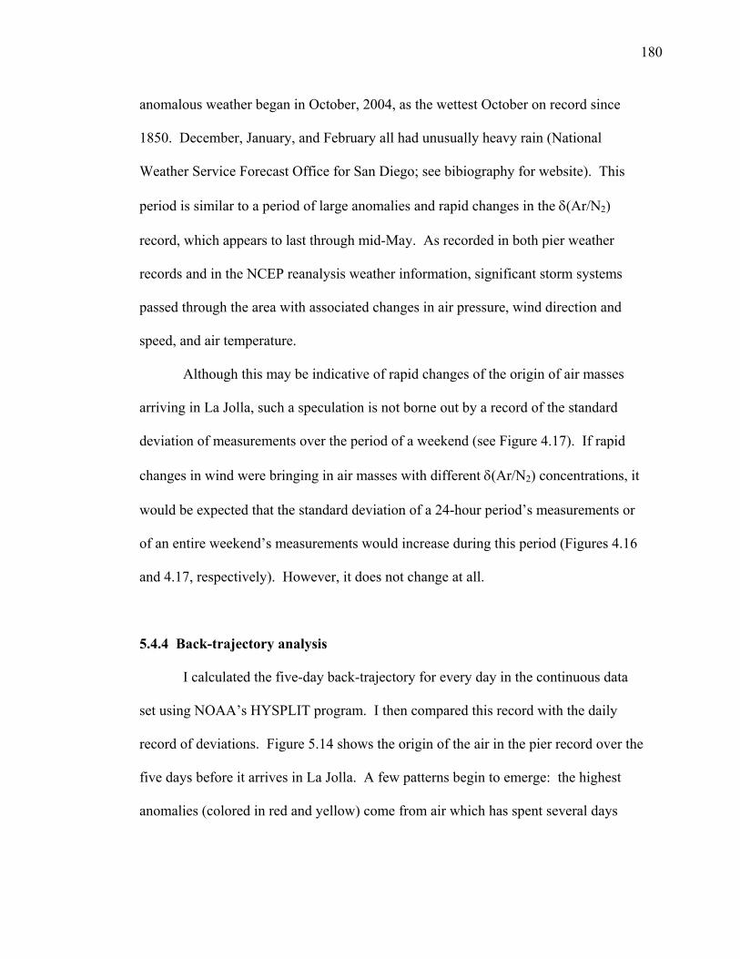
180
anomalous weather began in October, 2004, as the wettest October on record since
1850. December, January, and February all had unusually heavy rain (National
Weather Service Forecast Office for San Diego; see bibiography for website). This
period is similar to a period of large anomalies and rapid changes in the δ(Ar/N2)
record, which appears to last through mid-May. As recorded in both pier weather
records and in the NCEP reanalysis weather information, significant storm systems
passed through the area with associated changes in air pressure, wind direction and
speed, and air temperature.
Although this may be indicative of rapid changes of the origin of air masses
arriving in La Jolla, such a speculation is not borne out by a record of the standard
deviation of measurements over the period of a weekend (see Figure 4.17). If rapid
changes in wind were bringing in air masses with different δ(Ar/N2) concentrations, it
would be expected that the standard deviation of a 24-hour period’s measurements or
of an entire weekend’s measurements would increase during this period (Figures 4.16
and 4.17, respectively). However, it does not change at all.
5.4.4 Back-trajectory analysis
I calculated the five-day back-trajectory for every day in the continuous data
set using NOAA’s HYSPLIT program. I then compared this record with the daily
record of deviations. Figure 5.14 shows the origin of the air in the pier record over the
five days before it arrives in La Jolla. A few patterns begin to emerge: the highest
anomalies (colored in red and yellow) come from air which has spent several days
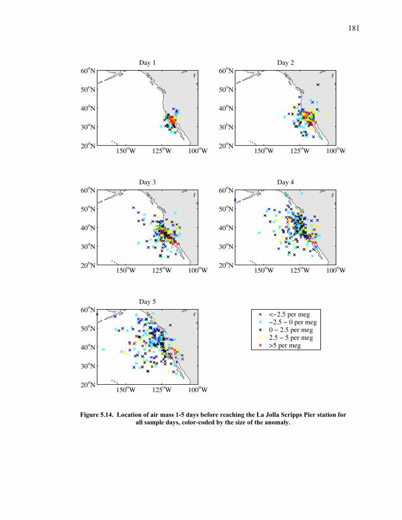
181
Day 1
150oW 125oW 100oW 20oN
30oN
40oN
50oN
60oN Day 2
150oW 125oW 100oW 20oN
30oN
40oN
50oN
60oN
Day 3
150oW 125oW 100oW 20oN
30oN
40oN
50oN
60oN Day 4
150oW 125oW 100oW 20oN
30oN
40oN
50oN
60oN
Day 5
150oW 125oW 100oW 20oN
30oN
40oN
50oN
60oN <−2.5 per meg−2.5 − 0 per meg0 − 2.5 per meg2.5 − 5 per meg>5 per meg
Figure 5.14. Location of air mass 1-5 days before reaching the La Jolla Scripps Pier station for all sample days, color-coded by the size of the anomaly.
182
along the California coast rather than being advected rapidly towards the station from
other areas. Air coming from due south tends to have anomalies between -2.5 and 2.5
per meg but not high anomalies, whereas the air coming from the north and west
shows both high and low anomalies.
The observation that the anomalies coming from the south tend to hover
around zero is likely due to the smaller annual cycle expected in lower latitudes, as the
air-sea heat flux cycle is also small. Any deviations due to variations in air-sea heat
flux, the amount of solar radiation received, or air or water temperature is likely to be
scaled accordingly. In contrast, air that is near the coast is probably exposed to areas
with the largest fluctuations in local Ar/N2 ratios, both because coastal upwelling
causes changes in air-sea heat flux, but also because upwelling areas may cause
unexpected changes in N2 and Ar fluxes due to the origin of the water. As mentioned
before, upwelling water tends to be high in nutrients and releases N2O and N2 to the
atmosphere (Nevison et al. 2004). Upwelling water also has Ar and N2 signatures of
the place where that water initially downwelled, rather than being at equilibrium with
local conditions. Just as oceans carry heat from low to high latitudes, they likely carry
Ar and N2. This flux should lead to a small zonal gradient in mean atmospheric
δ(Ar/N2) values whose size depends on the strength of the transport, with high values
in equatorial areas and low values at high latitudes. Thus, the origin of local water
masses near a station may be just as important as the origin of air masses arriving at
the station in understanding both seasonal patterns and anomalies. Air masses that
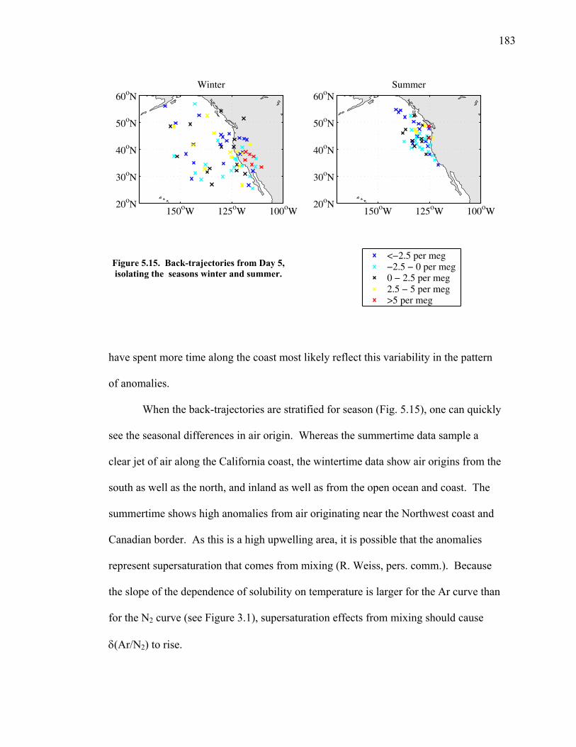
183
Winter
150oW 125oW 100oW 20oN
30oN
40oN
50oN
60oN Summer
150oW 125oW 100oW 20oN
30oN
40oN
50oN
60oN
Figure 5.15. Back-trajectories from Day 5, isolating the seasons winter and summer.
<−2.5 per meg−2.5 − 0 per meg0 − 2.5 per meg2.5 − 5 per meg>5 per meg
have spent more time along the coast most likely reflect this variability in the pattern
of anomalies.
When the back-trajectories are stratified for season (Fig. 5.15), one can quickly
see the seasonal differences in air origin. Whereas the summertime data sample a
clear jet of air along the California coast, the wintertime data show air origins from the
south as well as the north, and inland as well as from the open ocean and coast. The
summertime shows high anomalies from air originating near the Northwest coast and
Canadian border. As this is a high upwelling area, it is possible that the anomalies
represent supersaturation that comes from mixing (R. Weiss, pers. comm.). Because
the slope of the dependence of solubility on temperature is larger for the Ar curve than
for the N2 curve (see Figure 3.1), supersaturation effects from mixing should cause
δ(Ar/N2) to rise.
184
The winter days with air origins from inland tend to have large positive
anomalies. Representing stagnant air, these seven days have an average diurnal cycle
of about 2.2 per meg (not shown), more than twice as large as the estimated diurnal
cycle of about 1 per meg over the entire data set. Y. Adachi has shown night-time
accumulation of Ar near the ground in the desert leading to fractionation of up to 200
per meg (Y. Adachi and R. Keeling, pers. comm.). It is possible that these days are
measuring a pooling effect, in which a natural fractionation process over land leads to
more Ar near the surface of the earth
5.5 Possible instrumental problems
Possible remaining instrumental problems were discussed in Chapter 4. It is
probable that instrumental problems remain due to regular shutdown of the pierline on
a weekly basis for use in other research. The mean of any given weekend run or given
24-hour period has a standard deviation of about 2 per meg; the difference between
weekends can be much larger. The autocorrelation of the δ(Ar/N2) residuals in Figure
5.11 supports the conclusion that stopping the instrument for several days is
contributing to the jump in concentration: the autocorrelation drops on the order of 3-
4 days, increasing again for 5-8 days. This dip corresponds to the average length of a
weekend run before the instrument is shut off and is possibly caused by discrepancies
in the δ(Ar/N2) value between the end of one run and the start of the next.
185
5.6 Conclusions
A record of semi-continuous measurements of δ(Ar/N2), along with contiguous
measurements of δ(O2/N2) and CO2, now exists for 17 months at the Scripps Pier in
La Jolla, CA. This record shows a clear annual cycle of δ(Ar/N2) at this station,
defined to within 0.1 per meg, with the annual mean defined to within 0.2 per meg, It
also allows a close look at synoptic variability in the record. The lack of a good
explanation for even the largest anomalies in the δ(Ar/N2) record is a problem that will
most likely be resolved with longer datasets and upgrading to a continuous (rather than
semi-continuous) measurement system.. Regardless, this unique dataset will serve as
a basis for comparison for any other upcoming continuous measurement system. It
may also be important in analyzing results and continuing to make improvements in
existing flask programs.
The size of the annual cycle in atmospheric δ(Ar/N2) is within a range of
values expected by comparison with estimates based on changes in solubility and
seasonal air-sea heat flux estimates. Parallel measurements of CO2 and δ(O2/N2)
allow the annual δ(O2/N2) cycle to be broken into components due to air-sea heat flux,
land biology, and changes in ocean biology and dynamics. Although the strength of
these different components has been estimated in long-term records and in model
results, no other data set exists where the comparative strength of these components
can be broken down so clearly on a seasonal time scale.
In this dataset, the overall ratio between the part of the annual cycle due to
ocean dynamics and the part due to air-sea heat transport is smaller than expected
186
given comparison with other research predicting this ratio. However, it is possible that
these data demonstrate changes in the strength of different mechanisms on interannual
time scales; in 2004-2005, the annual cycle of ocean heat storage was larger than the
long-term mean. This observation may explain why the ratio is low over this period,
as the part of the oxygen cycle attributable to air-sea heat flux may be large relative to
the amount due to other ocean mechanisms. At this moment, any conclusions about
atmospheric δ(Ar/N2) based on this dataset are primarily restricted to seasonal time
scales and anything on interannual time scales is speculative. However, these results
give an indication of the importance of these measurements, especially in
understanding the strength of different mechanisms on interannual time scales.
5.7 Acknowledgements
I would like to acknowledge the NOAA Air Resources Laboratory (ARL) for
the provision of the HYSPLIT transport and dispersion model and READY website
(http://www.arl.noaa.gov/ready.html) used in this publication. The National Center
for Environmental Prediction (NCEP) reanalysis data was provided by the NOAA-
CIRES Climate Diagnostics Center, Boulder, Colorado, from their web site at
http://www.cdc.noaa.gov. The extended sea surface temperature dataset was provided
by the NOAA National Climatic Data Center, Asheville, North Carolina, at web site:
http://lwf.ncdc.noaa.gov/oa/climate/research/sst/sst.html. I also appreciate the help
from Bob Parker (SIO-IGPP) for help in dealing with time series analysis on data with
significant temporal gaps. Ray Weiss and Peter Salameh provided continuous data of

187
N2O and other atmospheric gases from their continuous measurement program at the
Scripps Pier, La Jolla, CA, as part of the Advanced Global Atmospheric Gases
Experiment (AGAGE) project.
188
5.8 Bibliography
Battle, M., M. Bender, M. B. Hendricks, D. T. Ho, R. Mika, G. McKinley, S.-M. Fan, T. Blaine, and R. F. Keeling. 2003. Measurements and models of the atmospheric Ar/N2 ratio. Geophys. Res. Lett. 30 (doi: 10.1029/2003GL017411).
Balkanski, Y., P. Monfray, M. Battle, and M. Heimann. 1999. Ocean primary
production derived from satellite data: An evaluation with atmospheric oxygen measurements. Glob. Biogeochem. Cycles 13: 257-271.
Barnett, T. P., D. W. Pierce, K. M. AchutaRao, P. J. Gleckler, B. D. Santer, J. M.
Gregory, and W. M. Washington. 2005. Penentration of human-induced warming into the world’s oceans. Science 309: 284-287.
Bender, M., T. Ellis, P. P. Tans, R. Francey, and D. Lowe. 1996. Variability in the
O2/N2 ratio of the southern hemisphere air, 1991-1994: Implications for the carbon cycle. Glob. Biogeochem. Cycles 10: 9-21.
Bopp, L., C. Le Quéré, M. Heimann, and A. C. Manning. 2002. Climate-induced
oceanic oxygen fluxes: Implications for the contemporary carbon budget. Glob. Biogeochem. Cycles 16 (doi: 10.1029/2001GB001445).
Burk, S. D. and W. T. Thompson. 1996. The summertime low level jet and marine
boundary layer structure along the California coast. Mon. Weather Rev. 124: 668-686.
Di Lorenzo, E., A. J. Miller, N. Schneider, and J. C. McWilliams. 2005. The
warming of the California Current System: Dynamics and ecosystem implications. J. Phys. Ocean. 35: 336-362.
Draxler, R.R. and Rolph, G.D., 2003. HYSPLIT (HYbrid Single-Particle Lagrangian
Integrated Trajectory) Model access via NOAA ARL READY Website (http://www.arl.noaa.gov/ready/hysplit4.html). NOAA Air Resources Laboratory, Silver Spring, MD.
Garcia, H. E. and R. F. Keeling. 2001. On the global oxygen anomaly and air-sea
flux. J. Geophys. Res. 106: 31,155-31,166. Garcia, H. E., T. P. Boyer, S. Levitus, R. A. Locarnini, and J. Antonov. 2005. On the
variability of dissolved oxygen and apparent oxygen utilization content for the upper world ocean: 1955 to 1998. Geophys. Res. Lett. 32 (doi: 10.1029/2004GL022286).
189
Gattuso, J.-P., M. Frankignoulle, and R. Wollast. 1998. Carbon and carbonate metabolism in coastal aquatic ecosystems. Ann. Rev. Ecol. Syst. 29: 405-434.
Gregg, W. W., M. E. Conkright, P. Ginoux, J. E. O’Reilly, and N. W. Casey. 2003.
Ocean primary production and climate: Global decadal changes. Geophys Res Lett 30: 1809 (doi: 10.1029/2003GL016889).
Hansen, J., L. Nazarenko, R. Ruedy, M. Sato, J. Willis, A. Del Genio, D. Koch, A.
Lacis, K. Lo, S. Menon, T. Novakov, J. Perlwitz, G. Russell, G. A. Schmidt, and N. Tausnev. 2005. Earth’s energy imbalance: confirmation and implications. Science 308: 1431-1435.
Keeling, R. F. 1988. Measuring correlations between atmospheric oxygen and carbon
dioxide mole fractions: A preliminary study in urban air. J. Atmos. Chem. 7: 153-176.
Keeling, R. F., T. Blaine, B. Paplawsky, L. Katz, C. Atwood, and T. Brockwell. 2004.
Measurement of changes in atmospheric Ar/N2 ratio using a rapid-switching, single-capillary mass spectrometer system. Tellus 56B: 322-388.
Keeling, R. F., and H. E. Garcia. 2002. The change in oceanic O2 inventory
associated with recent global warming. Proc. Nat. Acad. Sci. 99 (doi: 10.1073/pnas.122154899).
Keeling, R. F. and S. R. Shertz. 1992. Seasonal and interannual variations in
atmospheric oxygen and implications for the global carbon cycle. Nature 358: 723-727.
Keeling, R. F., B. B. Stephens, R. G. Najjar, S. C. Doney, D. Archer, and M.
Heimann. 1998. Seasonal variations in the atmospheric O2/N2 ratio in relation to kinetics of air-sea gas exchange. Glob. Biogeochem. Cycles 12: 141-163.
Levitus, S., J. Antonov, and T. Boyer. 2005. Warming of the world ocean, 1955-
2003. Geophys. Res. Lett. 32, L02604 (doi: 10.1029/2004GL021592). Lueker, T. J., R. F. Keeling, and M. K. Dubey. 2001. The oxygen to carbon dioxide
ratios observed in emissions from a wildfire in northern California. Geophys. Res. Lett. 28: 2413-2416.
Lueker, T. J., S. J. Walker, M. K. Vollmer, R. F. Keeling, C. D. Nevison, and R. F.
Weiss. 2003. Coastal upwelling air-sea fluxes revealed in atmospheric observations of O2/N2, CO2, and N2O. Geophys. Res. Lett. 30 (doi: 10.1029/2002GL016615).
190
Maier-Reimer, E., U. Mikolajewicz, and A. Winguth. 1996. Clim. Dyn. 12: 711-721. Manning, A. C. 2001. Temporal variability of atmospheric oxygen from both
continuous measurements and a flask sampling network: Tools for studying the global carbon cycle. Ph.D. thesis: University of California, San Diego, La Jolla, CA.
Matear, R. J. and A. C. Hirst. 2003. Long-term changes in dissolved oxygen
concentrations in the ocean caused by protracted global warming. Glob. Biogeochem. Cycles 17: 1125-1144 (doi: 10.1029/2002GB001997).
McKinley, G. A., M. J. Follows, and J. Marshall. 2000. Interannual variability of the
air-sea flux of oxygen in the North Atlantic. Geophys. Res. Lett. 27: 2933-2936.
McKinley, G. A., M. J. Follows, and J. Marshall. 2003. Interannual variability of air-
sea O2 fluxes and the determination of CO2 sinks using atmospheric O2/N2. Geophys. Res. Lett. 30 (doi: 10.1029/2002GL016044).
Mendelssohn, R., F. B. Schwing, and S. J. Bograd. 2004. Nonstationary seasonality
of upper ocean temperature in the California Current. J. Geophy. Res. 109 (doi: 10.1029/2004JC002330).
National Weather Service Forecast Office for San Diego:
http://newweb.wrh.noaa.gov/sgx/display_product.php?sid=SGX&pil=PNS) Nevison, C. D., T. J. Lueker, and R. F. Weiss. 2004. Quantifying the nitrous oxide
source from coastal upwelling. Glob. Biogeochem. Cycles 18 (doi: 10.1029/2003GB002110).
Peixoto, J. P. and A. H. Oort. 1992. Physics of Climate. American Institute of
Physics: New York, NY. Prinn, R. G., R. F. Weiss, P. J. Fraser, P. G. Simmonds, D. M. Cunnold, F. N. Alyea,
S. O’Doherty, P. Salameh, B. R. Miller, J. Huang, R. H. J. Wang, D. E. Hartley, C. Harth, L. P. Steele, G. Sturrock, P. M. Midgley, and A. McCulloch. 2000. A history of chemically and radiatively important gases in air deduced from ALE/GAGE/AGAGE. J. Geophys. Res. 105: 17,751-17,792.
Rogers, D. P., C. E. Dorman, K. A. Edwards, I. M. Brooks, W. K. Melville, S. D.
Burk, W. T. Thompson, T. Holt, L. M. Strom, M. Tjernstrom, B. Grisogono, J. M. Bane, W. A. Nuss, B. M. Morley, and A. J. Schanot. 1998. Highlights of Coastal Waves 1996. Bull. Am. Meteorol. Soc. 79: 1307-1326.
191
Rolph, G.D. 2003. Real-time Environmental Applications and Display System
(READY) Website (http://www.arl.noaa.gov/ready/hysplit4.html). NOAA Air Resources Laboratory, Silver Spring, MD.
Sarmiento, J. L., T. M. C. Hughes, R. J. Stouffer, and S. Manabe. 1998. Simulated
response of the ocean carbon cycle to anthropogenic climate warming. Nature 393: 245-249.
Smith, T. M. and R. W. Reynolds. 2003. Extended reconstruction of global sea
surface temperatures based on COADS data (1854-1997). J. Clim. 16: 1495-1510.
Smith, T. M. and R. W. Reynolds. 2004. Improved extended reconstruction of SST
(1985-1997). J. Clim. 17: 2466-2477. Snyder, M. A., L. C. Sloan, N. S. Diffenbaugh, and J. L. Bell. 2003. Future climate
change and upwelling in the California Current. Geophys. Res. Lett. 30: 1823 (doi: 10.1029/2003GL017647).
Stephens, B. B., R. F. Keeling, M. Heimann, K. D. Six, R. Murnane, and K. Caldiera.
1998. Testing global ocean carbon cycle models using measurements of atmospheric O2 and CO2 concentration. Glob. Biogeochem. Cycles 12: 213-230.
Weiss, R. F. 1970. The solubility of nitrogen, oxygen, and argon in water and
seawater. Deep-Sea Res. 17: 721-735.
192
Appendix 1
Determination of interference and nonlinearity correction factors
A1.1. Introduction
The measurements of a particular species in the mass spectrometer are not
necessarily the actual concentration values, because of interferences from other gases
or other effects. In order to develop fits between mass spectrometer measurements
and the true values of the concentration of a species, named the S2 values, we bled gas
of known mixtures of CO2, O2, and Ar into the working tank of the mass spectrometer
and calculated linear relationships between the measured and expected concentrations
of particular gases. We used 99% pure CO2, a mixture of CO2 and O2, and a mixture
of CO2 and Ar, bled into two separate working tanks. The mixing ratios of the tanks
used are listed in Table A1.1.
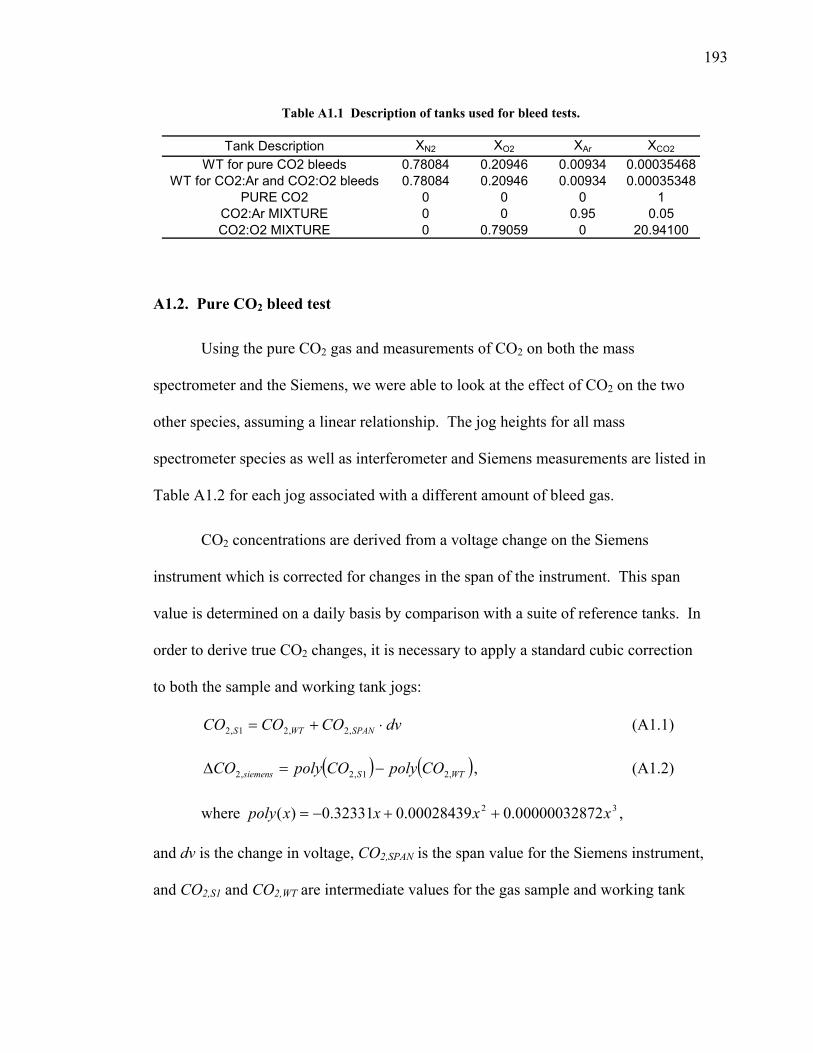
193
Table A1.1 Description of tanks used for bleed tests.
Tank Description XN2 XO2 XAr XCO2
WT for pure CO2 bleeds 0.78084 0.20946 0.00934 0.00035468WT for CO2:Ar and CO2:O2 bleeds 0.78084 0.20946 0.00934 0.00035348
PURE CO2 0 0 0 1CO2:Ar MIXTURE 0 0 0.95 0.05CO2:O2 MIXTURE 0 0.79059 0 20.94100
A1.2. Pure CO2 bleed test
Using the pure CO2 gas and measurements of CO2 on both the mass
spectrometer and the Siemens, we were able to look at the effect of CO2 on the two
other species, assuming a linear relationship. The jog heights for all mass
spectrometer species as well as interferometer and Siemens measurements are listed in
Table A1.2 for each jog associated with a different amount of bleed gas.
CO2 concentrations are derived from a voltage change on the Siemens
instrument which is corrected for changes in the span of the instrument. This span
value is determined on a daily basis by comparison with a suite of reference tanks. In
order to derive true CO2 changes, it is necessary to apply a standard cubic correction
to both the sample and working tank jogs:
dvCOCOCO SPANWTS ⋅+= ,2,21,2 (A1.1)
( ) ( )WTSsiemens COpolyCOpolyCO ,21,2,2 −=Δ , (A1.2)
where 32 20000003287.000028439.032331.0)( xxxxpoly ++−= ,
and dv is the change in voltage, CO2,SPAN is the span value for the Siemens instrument,
and CO2,S1 and CO2,WT are intermediate values for the gas sample and working tank
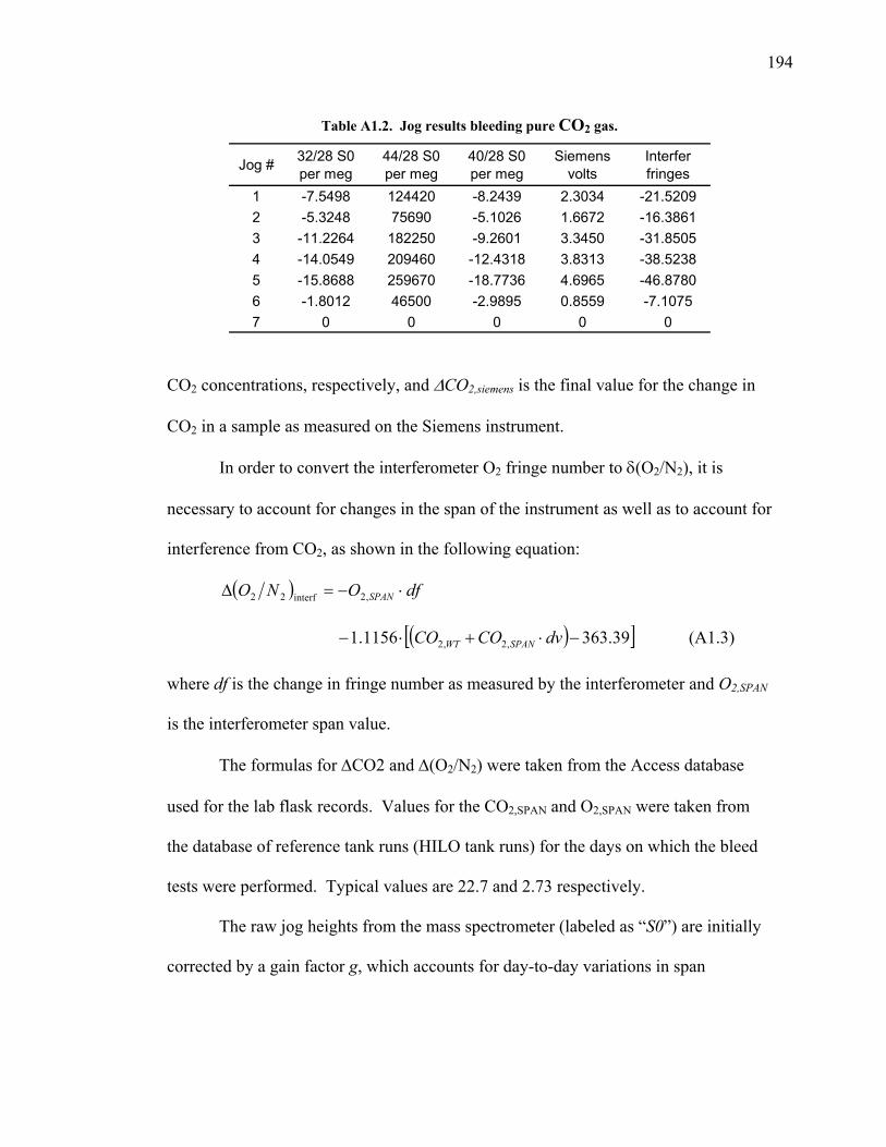
194
Table A1.2. Jog results bleeding pure CO2 gas.
Jog # 32/28 S0 per meg
44/28 S0 per meg
40/28 S0 per meg
Siemens volts
Interfer fringes
1 -7.5498 124420 -8.2439 2.3034 -21.52092 -5.3248 75690 -5.1026 1.6672 -16.38613 -11.2264 182250 -9.2601 3.3450 -31.85054 -14.0549 209460 -12.4318 3.8313 -38.52385 -15.8688 259670 -18.7736 4.6965 -46.87806 -1.8012 46500 -2.9895 0.8559 -7.10757 0 0 0 0 0
CO2 concentrations, respectively, and ΔCO2,siemens is the final value for the change in
CO2 in a sample as measured on the Siemens instrument.
In order to convert the interferometer O2 fringe number to δ(O2/N2), it is
necessary to account for changes in the span of the instrument as well as to account for
interference from CO2, as shown in the following equation:
( ) dfONO SPAN ⋅−=Δ ,2interf22
( )[ ]39.3631156.1 ,2,2 −⋅+⋅− dvCOCO SPANWT (A1.3)
where df is the change in fringe number as measured by the interferometer and O2,SPAN
is the interferometer span value.
The formulas for ΔCO2 and Δ(O2/N2) were taken from the Access database
used for the lab flask records. Values for the CO2,SPAN and O2,SPAN were taken from
the database of reference tank runs (HILO tank runs) for the days on which the bleed
tests were performed. Typical values are 22.7 and 2.73 respectively.
The raw jog heights from the mass spectrometer (labeled as “S0”) are initially
corrected by a gain factor g, which accounts for day-to-day variations in span
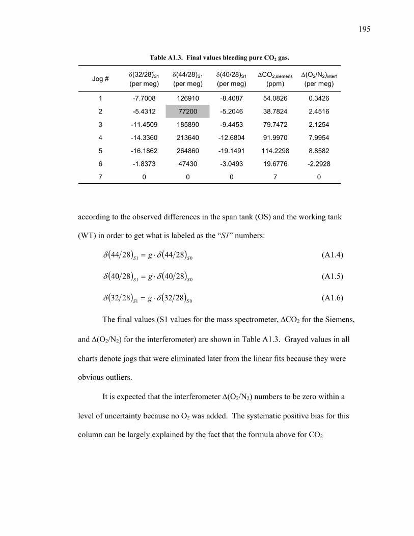
195
Table A1.3. Final values bleeding pure CO2 gas.
Jog # δ(32/28)S1
(per meg)δ(44/28)S1
(per meg)δ(40/28)S1
(per meg)ΔCO2,siemens
(ppm)Δ(O2/N2)interf
(per meg)
1 -7.7008 126910 -8.4087 54.0826 0.3426
2 -5.4312 77200 -5.2046 38.7824 2.4516
3 -11.4509 185890 -9.4453 79.7472 2.1254
4 -14.3360 213640 -12.6804 91.9970 7.9954
5 -16.1862 264860 -19.1491 114.2298 8.8582
6 -1.8373 47430 -3.0493 19.6776 -2.2928
7 0 0 0 7 0
according to the observed differences in the span tank (OS) and the working tank
(WT) in order to get what is labeled as the “S1” numbers:
( ) ( ) 01 28442844 SS g δδ ⋅= (A1.4)
( ) ( ) 01 28402840 SS g δδ ⋅= (A1.5)
( ) ( ) 01 28322832 SS g δδ ⋅= (A1.6)
The final values (S1 values for the mass spectrometer, ΔCO2 for the Siemens,
and Δ(O2/N2) for the interferometer) are shown in Table A1.3. Grayed values in all
charts denote jogs that were eliminated later from the linear fits because they were
obvious outliers.
It is expected that the interferometer Δ(O2/N2) numbers to be zero within a
level of uncertainty because no O2 was added. The systematic positive bias for this
column can be largely explained by the fact that the formula above for CO2
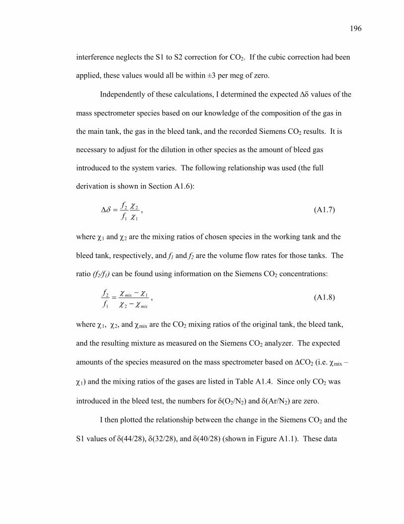
196
interference neglects the S1 to S2 correction for CO2. If the cubic correction had been
applied, these values would all be within ±3 per meg of zero.
Independently of these calculations, I determined the expected Δδ values of the
mass spectrometer species based on our knowledge of the composition of the gas in
the main tank, the gas in the bleed tank, and the recorded Siemens CO2 results. It is
necessary to adjust for the dilution in other species as the amount of bleed gas
introduced to the system varies. The following relationship was used (the full
derivation is shown in Section A1.6):
1
2
1
2
χχδ
ff
=Δ , (A1.7)
where χ1 and χ2 are the mixing ratios of chosen species in the working tank and the
bleed tank, respectively, and f1 and f2 are the volume flow rates for those tanks. The
ratio (f2/f1) can be found using information on the Siemens CO2 concentrations:
mix
mix
ff
χχχχ
−−
=2
1
1
2 , (A1.8)
where χ1, χ2, and χmix are the CO2 mixing ratios of the original tank, the bleed tank,
and the resulting mixture as measured on the Siemens CO2 analyzer. The expected
amounts of the species measured on the mass spectrometer based on ΔCO2 (i.e. χmix –
χ1) and the mixing ratios of the gases are listed in Table A1.4. Since only CO2 was
introduced in the bleed test, the numbers for δ(O2/N2) and δ(Ar/N2) are zero.
I then plotted the relationship between the change in the Siemens CO2 and the
S1 values of δ(44/28), δ(32/28), and δ(40/28) (shown in Figure A1.1). These data
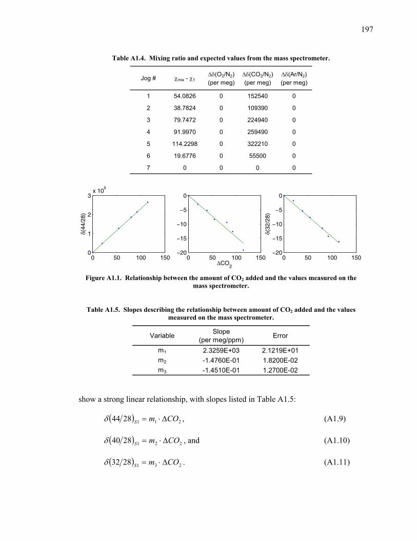
197
Table A1.4. Mixing ratio and expected values from the mass spectrometer.
Jog # χmix - χ1Δδ(O2/N2) (per meg)
Δδ(CO2/N2) (per meg)
Δδ(Ar/N2) (per meg)
1 54.0826 0 152540 0
2 38.7824 0 109390 0
3 79.7472 0 224940 0
4 91.9970 0 259490 0
5 114.2298 0 322210 0
6 19.6776 0 55500 0
7 0 0 0 0
0 50 100 1500
1
2
3x 10
5
δ(44
/28)
0 50 100 150−20
−15
−10
−5
0
ΔCO2
0 50 100 150−20
−15
−10
−5
0
δ(32
/28)
Figure A1.1. Relationship between the amount of CO2 added and the values measured on the
mass spectrometer.
Table A1.5. Slopes describing the relationship between amount of CO2 added and the values measured on the mass spectrometer.
Variable Slope (per meg/ppm) Error
m1 2.3259E+03 2.1219E+01m2 -1.4760E-01 1.8200E-02m3 -1.4510E-01 1.2700E-02
show a strong linear relationship, with slopes listed in Table A1.5:
( ) 2112844 COmS Δ⋅=δ , (A1.9)
( ) 2212840 COmS Δ⋅=δ , and (A1.10)
( ) 2312832 COmS Δ⋅=δ . (A1.11)
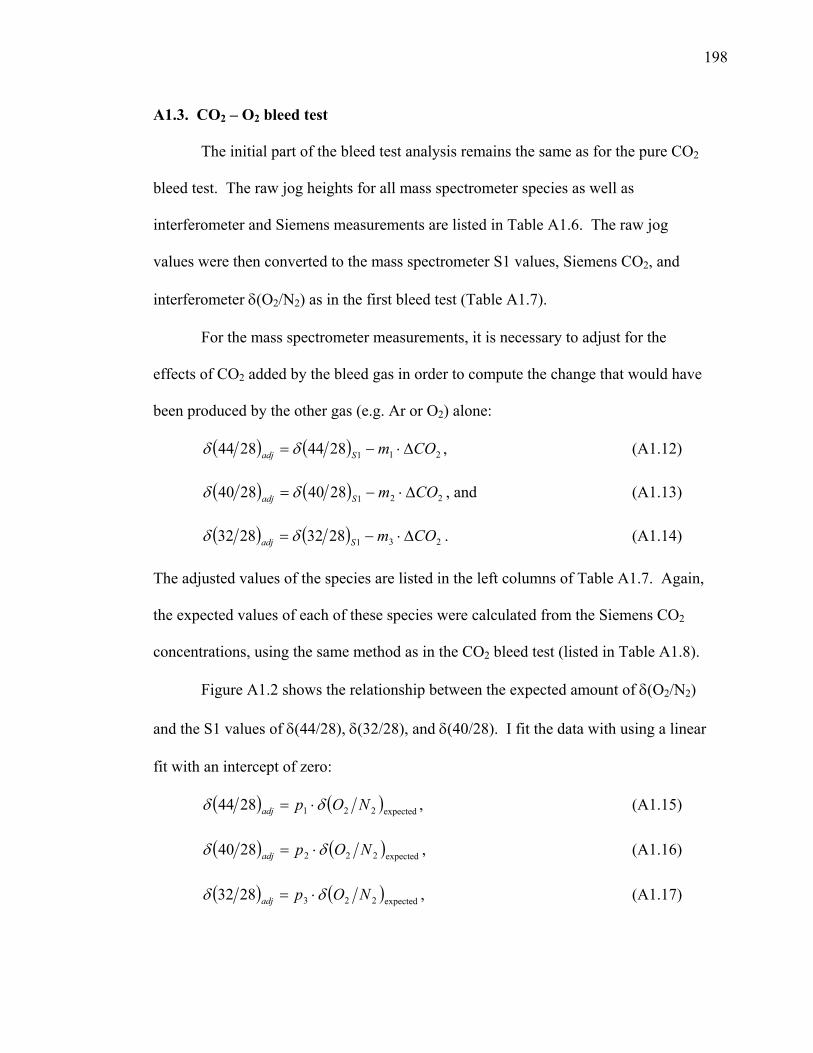
198
A1.3. CO2 – O2 bleed test
The initial part of the bleed test analysis remains the same as for the pure CO2
bleed test. The raw jog heights for all mass spectrometer species as well as
interferometer and Siemens measurements are listed in Table A1.6. The raw jog
values were then converted to the mass spectrometer S1 values, Siemens CO2, and
interferometer δ(O2/N2) as in the first bleed test (Table A1.7).
For the mass spectrometer measurements, it is necessary to adjust for the
effects of CO2 added by the bleed gas in order to compute the change that would have
been produced by the other gas (e.g. Ar or O2) alone:
( ) ( ) 21128442844 COmSadj Δ⋅−= δδ , (A1.12)
( ) ( ) 22128402840 COmSadj Δ⋅−= δδ , and (A1.13)
( ) ( ) 23128322832 COmSadj Δ⋅−= δδ . (A1.14)
The adjusted values of the species are listed in the left columns of Table A1.7. Again,
the expected values of each of these species were calculated from the Siemens CO2
concentrations, using the same method as in the CO2 bleed test (listed in Table A1.8).
Figure A1.2 shows the relationship between the expected amount of δ(O2/N2)
and the S1 values of δ(44/28), δ(32/28), and δ(40/28). I fit the data with using a linear
fit with an intercept of zero:
( ) ( )expected2212844 NOpadj δδ ⋅= , (A1.15)
( ) ( )expected2222840 NOpadj δδ ⋅= , (A1.16)
( ) ( )expected2232832 NOpadj δδ ⋅= , (A1.17)
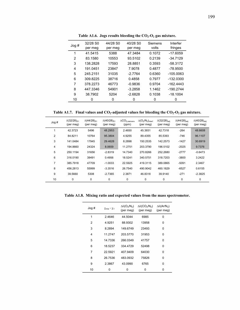
199
Table A1.6. Jogs results bleeding the CO2-O2 gas mixture.
Jog # 32/28 S0 per meg
44/28 S0 per meg
40/28 S0 per meg
Siemens volts
Interfer fringes
1 41.5415 5388 47.3484 0.1072 -17.60592 83.1580 10553 93.5102 0.2139 -34.71293 138.2828 17593 28.8851 0.3593 -58.31724 191.0451 23847 7.9078 0.4877 -78.95005 245.2151 31035 -2.7764 0.6360 -105.00636 309.8225 38716 0.4858 0.7977 -132.03007 378.2273 46773 -0.9836 0.9704 -162.44438 447.3346 54901 -3.2858 1.1462 -190.27449 38.7902 5204 -2.6828 0.1038 -18.100410 0 0 0 0 0
Table A1.7. Final values and CO2-adjusted values for bleeding the CO2-O2 gas mixture.
Jog # δ(32/28)S1
(per meg)δ(44/28)S1
(per meg)δ(40/28)S1
(per meg)ΔCO2,siemens
(ppm)Δ(O2/N2)interf
(per meg)δ(32/28)adj
(per meg)δ(44/28)adj
(per meg)δ(40/28)adj
(per meg)
1 42.3723 5496 48.2953 2.4650 45.3931 42.7318 -264 48.6608
2 84.8211 10764 95.3804 4.9255 89.4355 85.5393 -746 96.1107
3 141.0484 17945 29.4628 8.2898 150.2535 142.2573 -1427 30.6919
4 194.8660 24324 8.0659 11.2751 203.3790 196.5102 -2025 9.7376
5 250.1194 31656 -2.8319 14.7340 270.8266 252.2680 -2777 -0.6473
6 316.0190 39491 0.4956 18.5241 340.5751 318.7203 -3800 3.2422
7 385.7918 47709 -1.0033 22.5925 419.3115 389.0865 -5091 2.3467
8 456.2813 55999 -3.3516 26.7540 490.9042 460.1829 -6527 0.6155
9 39.5660 5308 -2.7365 2.3871 46.8318 39.9140 -271 -2.3825
10 0 0 0 0 0 0 0 0
Table A1.8. Mixing ratio and expected values from the mass spectrometer.
Jog # χmix - χ1Δδ(O2/N2) (per meg)
Δδ(CO2/N2) (per meg)
Δδ(Ar/N2) (per meg)
1 2.4646 44.5044 6985 0
2 4.9251 88.9302 13958 0
3 8.2894 149.6749 23493 0
4 11.2747 203.5770 31953 0
5 14.7336 266.0349 41757 0
6 18.5237 334.4729 52498 0
7 22.5921 407.9409 64030 0
8 26.7536 483.0932 75826 0
9 2.3867 43.0990 6765 0
10 0 0 0 0
200
0 200 400 600−8000
−6000
−4000
−2000
0
δ(44
/28)
adj
0 200 400 6000
200
400
600
δ(32
/28)
adj
0 200 400 600−4
−2
0
2
4
δ(40
/28)
adj
Expected δ(O2/N
2)
Figure A1.2. Relationship between the expected mass spectrometer measurement of the amount of δ(O2/N2) added and the values measured on the mass spectrometer.
Table A1.9. Slopes describing the relationship between the expected mass spectrometer measurement of the amount of δ(O2/N2) added and the values measured on the mass
spectrometer.
Variable Slope (per meg/ppm) Error
p1 -1.2089E+01 1.8713E+00p2 3.5000E-03 1.0600E-02p3 9.5330E-01 6.2000E-03
0 100 200 300 400 5000
100
200
300
400
500
Expected δ(O2/N
2) (per meg)
Inte
rfer
omet
er Δ
(O2/N
2) (p
er m
eg)
Slope = 1.0183
Figure A1.3. Linear fit between the expected δ(O2/N2) values and measured Interferometer
δ(O2/N2) values testing the O2 span calculations.
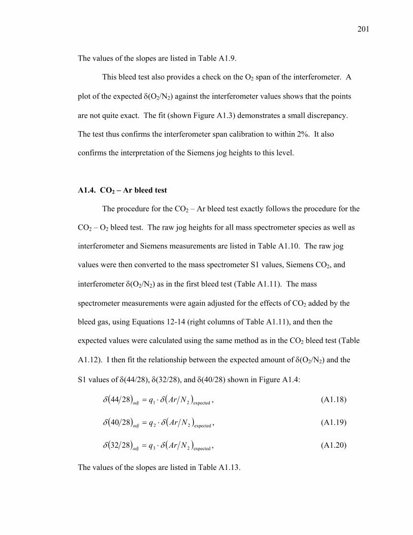
201
The values of the slopes are listed in Table A1.9.
This bleed test also provides a check on the O2 span of the interferometer. A
plot of the expected δ(O2/N2) against the interferometer values shows that the points
are not quite exact. The fit (shown Figure A1.3) demonstrates a small discrepancy.
The test thus confirms the interferometer span calibration to within 2%. It also
confirms the interpretation of the Siemens jog heights to this level.
A1.4. CO2 – Ar bleed test
The procedure for the CO2 – Ar bleed test exactly follows the procedure for the
CO2 – O2 bleed test. The raw jog heights for all mass spectrometer species as well as
interferometer and Siemens measurements are listed in Table A1.10. The raw jog
values were then converted to the mass spectrometer S1 values, Siemens CO2, and
interferometer δ(O2/N2) as in the first bleed test (Table A1.11). The mass
spectrometer measurements were again adjusted for the effects of CO2 added by the
bleed gas, using Equations 12-14 (right columns of Table A1.11), and then the
expected values were calculated using the same method as in the CO2 bleed test (Table
A1.12). I then fit the relationship between the expected amount of δ(O2/N2) and the
S1 values of δ(44/28), δ(32/28), and δ(40/28) shown in Figure A1.4:
( ) ( )expected212844 NArqadj δδ ⋅= , (A1.18)
( ) ( )expected222840 NArqadj δδ ⋅= , (A1.19)
( ) ( )expected232832 NArqadj δδ ⋅= , (A1.20)
The values of the slopes are listed in Table A1.13.
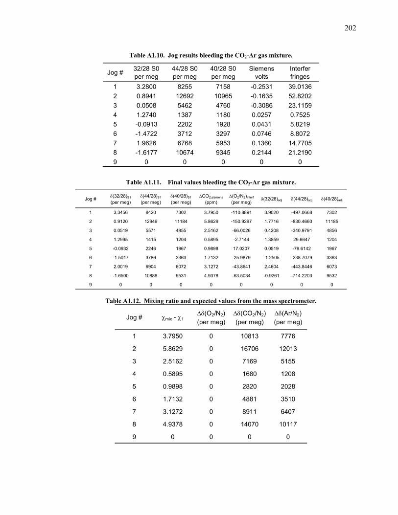
202
Table A1.10. Jog results bleeding the CO2-Ar gas mixture.
Jog # 32/28 S0 per meg
44/28 S0 per meg
40/28 S0 per meg
Siemens volts
Interfer fringes
1 3.2800 8255 7158 -0.2531 39.01362 0.8941 12692 10965 -0.1635 52.82023 0.0508 5462 4760 -0.3086 23.11594 1.2740 1387 1180 0.0257 0.75255 -0.0913 2202 1928 0.0431 5.82196 -1.4722 3712 3297 0.0746 8.80727 1.9626 6768 5953 0.1360 14.77058 -1.6177 10674 9345 0.2144 21.21909 0 0 0 0 0
Table A1.11. Final values bleeding the CO2-Ar gas mixture.
Jog # δ(32/28)S1
(per meg)δ(44/28)S1
(per meg)δ(40/28)S1
(per meg)ΔCO2,siemens
(ppm)Δ(O2/N2)interf
(per meg)δ(32/28)adj δ(44/28)adj δ(40/28)adj
1 3.3456 8420 7302 3.7950 -110.8891 3.9020 -497.0668 7302
2 0.9120 12946 11184 5.8629 -150.9297 1.7716 -830.4660 11185
3 0.0519 5571 4855 2.5162 -66.0026 0.4208 -340.9791 4856
4 1.2995 1415 1204 0.5895 -2.7144 1.3859 29.6647 1204
5 -0.0932 2246 1967 0.9898 17.0207 0.0519 -79.6142 1967
6 -1.5017 3786 3363 1.7132 -25.9879 -1.2505 -238.7079 3363
7 2.0019 6904 6072 3.1272 -43.8641 2.4604 -443.8446 6073
8 -1.6500 10888 9531 4.9378 -63.5034 -0.9261 -714.2203 9532
9 0 0 0 0 0 0 0 0
Table A1.12. Mixing ratio and expected values from the mass spectrometer.
Jog # χmix - χ1Δδ(O2/N2) (per meg)
Δδ(CO2/N2) (per meg)
Δδ(Ar/N2) (per meg)
1 3.7950 0 10813 7776
2 5.8629 0 16706 12013
3 2.5162 0 7169 5155
4 0.5895 0 1680 1208
5 0.9898 0 2820 2028
6 1.7132 0 4881 3510
7 3.1272 0 8911 6407
8 4.9378 0 14070 10117
9 0 0 0 0
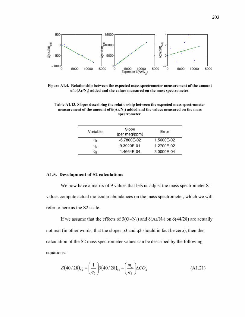
203
0 5000 10000 15000−1000
−500
0
500
δ(44
/28)
adj
0 5000 10000 15000−2
0
2
4
δ(32
/28)
adj
0 5000 10000 150000
5000
10000
15000
δ(40
/28)
adj
Expected δ(Ar/N2)
Figure A1.4. Relationship between the expected mass spectrometer measurement of the amount of δ(Ar/N2) added and the values measured on the mass spectrometer.
Table A1.13. Slopes describing the relationship between the expected mass spectrometer measurement of the amount of δ(Ar/N2) added and the values measured on the mass
spectrometer.
Variable Slope (per meg/ppm) Error
q1 -6.7800E-02 1.5600E-02q2 9.3920E-01 1.2700E-02q3 1.4664E-04 3.0000E-04
A1.5. Development of S2 calculations
We now have a matrix of 9 values that lets us adjust the mass spectrometer S1
values compute actual molecular abundances on the mass spectrometer, which we will
refer to here as the S2 scale.
If we assume that the effects of δ(O2/N2) and δ(Ar/N2) on δ(44/28) are actually
not real (in other words, that the slopes p3 and q2 should in fact be zero), then the
calculation of the S2 mass spectrometer values can be described by the following
equations:
( ) ( ) 22
21
22 28/40128/40 CO
qm
q SS Δ⎟⎟⎠
⎞⎜⎜⎝
⎛−⎟⎟
⎠
⎞⎜⎜⎝
⎛= δδ (A1.21)
204
( ) ( ) 23
31
32 28/32128/32 CO
pm
p SS Δ⎟⎟⎠
⎞⎜⎜⎝
⎛−⎟⎟
⎠
⎞⎜⎜⎝
⎛= δδ (A1.22)
This suggestion assumes that the gain factor is already included in the S1 values and
therefore does not need to appear in the matrix. Relating the S2 values to ΔCO2 is
better than relating them to δ(CO2/N2) because there are long-term stability standards
in CO2 mole fraction but not in δ(CO2/N2).
A1.6. A note on the derivation of the expected Mass Spectrometer ratios
We calculated the expected values of the mass spectrometer species based on
our knowledge of the composition of the gas in the main tank, the gas in the bleed
tank, and the recorded Siemens CO2 results. We had to adjust for the dilution in other
species as the amount of bleed gas introduced to the system varies. The development
of this relationship is given below.
The mixing ratio of a given species in the mixture of tank gas and bleed gas is
the following:
,1
1
2
21
21
21
2211
ffff
ffff
mix
+
+=
++
=χχ
χχχ (A1.23)
where χ1, χ2, and χmix are the respective mixing ratios of a particular species of the
tank gas, bleed gas, and resultant mixture, and f1 and f2 are the volume flows of the
two gases. Assuming that we are introducing no nitrogen into the system through the
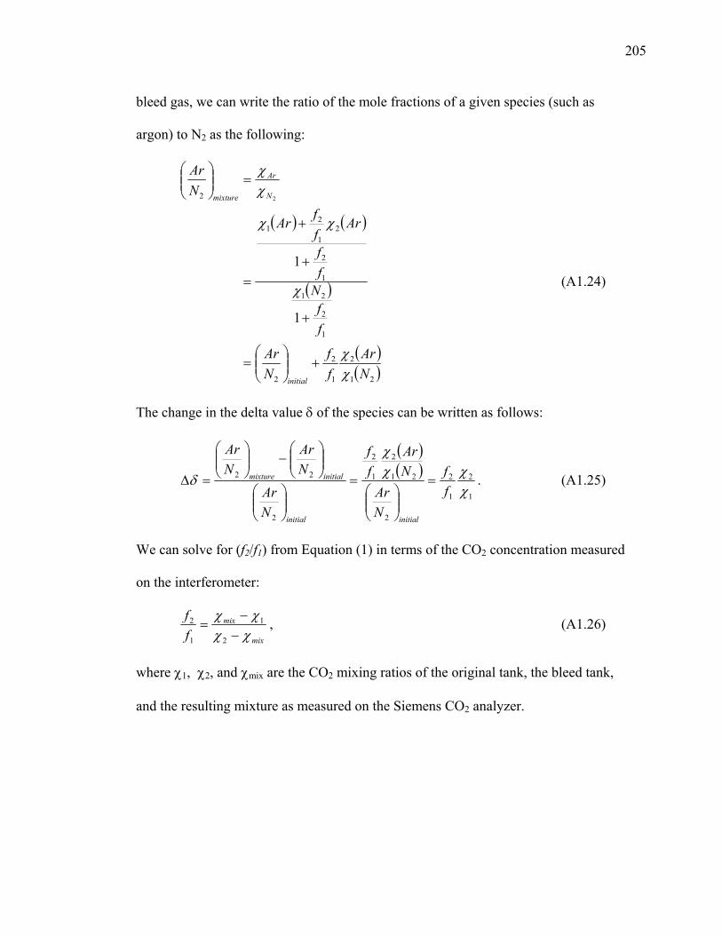
205
bleed gas, we can write the ratio of the mole fractions of a given species (such as
argon) to N2 as the following:
( ) ( )
( )
( )( )21
2
1
2
2
1
2
21
1
2
21
21
2
1
1
2
NAr
ff
NAr
ff
Nff
ArffAr
NAr
initial
N
Ar
mixture
χχ
χ
χχ
χχ
+⎟⎟⎠
⎞⎜⎜⎝
⎛=
+
+
+
=
=⎟⎟⎠
⎞⎜⎜⎝
⎛
(A1.24)
The change in the delta value δ of the species can be written as follows:
( )( )
1
2
1
2
2
21
2
1
2
2
22
χχχ
χ
δff
NAr
NAr
ff
NAr
NAr
NAr
initialinitial
initialmixture =
⎟⎟⎠
⎞⎜⎜⎝
⎛=
⎟⎟⎠
⎞⎜⎜⎝
⎛
⎟⎟⎠
⎞⎜⎜⎝
⎛−⎟⎟
⎠
⎞⎜⎜⎝
⎛
=Δ . (A1.25)
We can solve for (f2/f1) from Equation (1) in terms of the CO2 concentration measured
on the interferometer:
mix
mix
ff
χχχχ
−−
=2
1
1
2 , (A1.26)
where χ1, χ2, and χmix are the CO2 mixing ratios of the original tank, the bleed tank,
and the resulting mixture as measured on the Siemens CO2 analyzer.
206
Appendix 2
Timeline of instrument development
A2.1 Setup changes during development
1. Tests on roofline began 09/03. Described in lab notebook. Used ¼” Synflex
tubing on a tower on the roof, snaked tubing down into interferometer room.
2. Pierline began 11/14/04. Assumed use of existing lines of ½” Synflex tubing.
Intake located near east end (shore-side) of pier.
3. Stopped use of fridge on 12/15/2003. Subsequently relying only on -80oC
chiller to get rid of water in the sample air.
4. Aspirator installed 1/20/04. Borrowed from Cayan’s group.
5. Mass spec reference tank exhausted and replaced on 2/4/2004. No diptube on
either old or new tank.
6. 3 ¼” Synflex tubing lines were installed between 3/8/04-3/12/04. Stopped
using ½” lines for any pierline tests. Two dedicated lines for the pierline setup
207
lead into the interferometer lab, third line plumbed to go into Tim’s equipment
across the hall.
7. Mass Spec tuned on 5/5/04.
8. Hi Span exhausted and replaced on 5/7/04. No diptube in either old or new
tank.
9. Moved cold traps to before pumps on 5/14/04. Was having significant
problems with a failure rate of the pressure controller and the pumps associated
with water and salt entering the system. In this setup, much of the
water/particulates in the air freezes out before reaching the pump.
10. Swapped 1½” OD cold traps in for 1” OD cold traps on 5/21/04 in order to
extend the length of time before cold traps need to be changed. The 1” OD
traps were sometimes lasting only 22 hours before freezing up; the larger traps
last almost twice as long.
11. Introduced first diptube pierline working tank on 5/24/05 when the last tank
was exhausted and needed to be replaced. Diptube tanks described in Section
4.3.2.
12. Introduced two solenoid 3-port, 2 position valves and timer on 5/30/04 in
order to switch automatically between cold traps in order to enhance trap
lifetime. Using only one pierline, one valve was located before the two traps,
one valve behind the traps. Both would switch automatically at the same time
in order to switch the pierline from one trap to the other.
208
13. Phased out trap switch and returned to two-line system on 7/28/05, each line
with its own dedicated trap. As of this date, the system looks like the
description and schematic in Chapter 4. This system of two lines sampled
every other hour has two advantages: can test changes in one line against the
other (i.e. in testing a solar shield against the aspirator), and also can help
recognize and diagnose problems in one line more rapidly.
14. Power failure on 11/15/04 18;30. Machine shut down, not fully operational
again through the next day.
15. Mass spec reference tank exhausted and replaced on 12/10/04 12:00. Neither
old nor new tank has a diptube.
16. Low span tank exhausted and replaced on 1/28/05. Old tank does not have
diptube; new tank does have diptube. Note: Neither high nor oxspan tanks
have diptubes.
17. Oxspan tank exhausted and replaced on 2/24/04. Neither old nor new tanks
have diptubes. New working tanks for flask operation are installed; both have
diptubes.
A2.2 Notes on particular tests
A2.2.1 Roofline tests 17-09-03 2 days LowWT leaks, failed HILO 29-09-03 2 days LowWT leaks 03-10-03 4 days LowWT 24-10-03 2 days LowWT 31-10-03 4 days LowWT 07-11-03 4 days LowWT Have record of boiler switches during this time
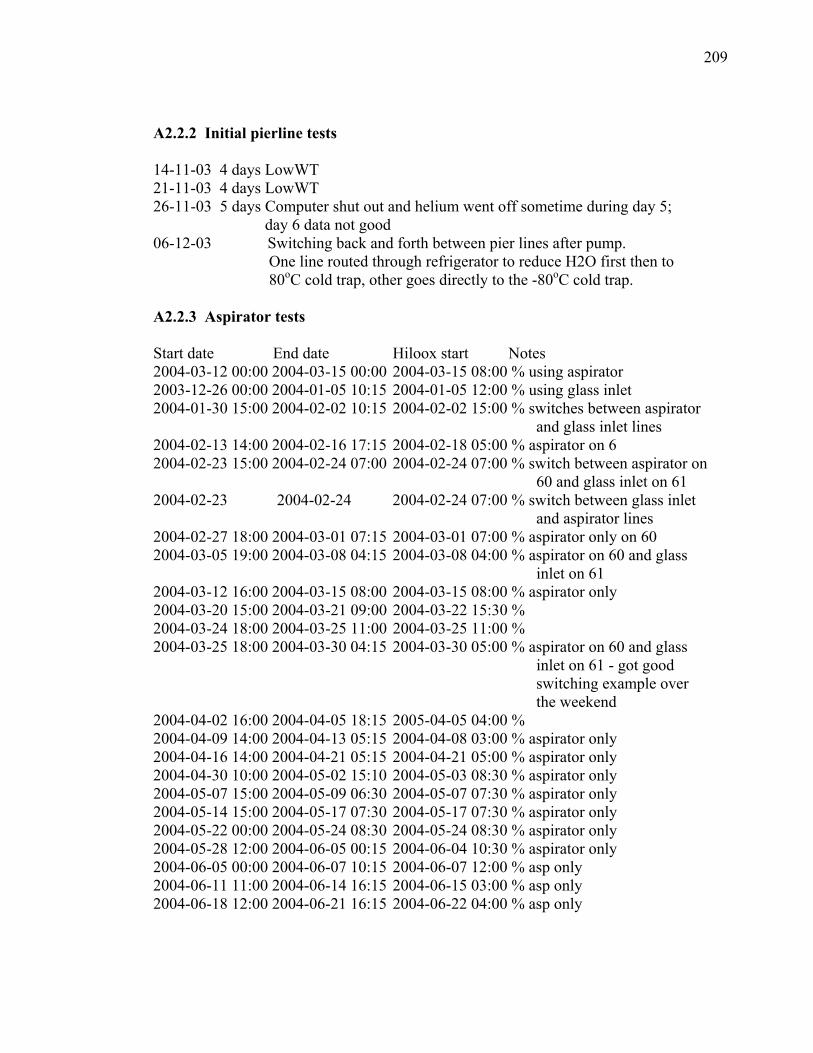
209
A2.2.2 Initial pierline tests 14-11-03 4 days LowWT 21-11-03 4 days LowWT 26-11-03 5 days Computer shut out and helium went off sometime during day 5;
day 6 data not good 06-12-03 Switching back and forth between pier lines after pump.
One line routed through refrigerator to reduce H2O first then to 80oC cold trap, other goes directly to the -80oC cold trap.
A2.2.3 Aspirator tests Start date End date Hiloox start Notes 2004-03-12 00:00 2004-03-15 00:00 2004-03-15 08:00 % using aspirator 2003-12-26 00:00 2004-01-05 10:15 2004-01-05 12:00 % using glass inlet 2004-01-30 15:00 2004-02-02 10:15 2004-02-02 15:00 % switches between aspirator
and glass inlet lines 2004-02-13 14:00 2004-02-16 17:15 2004-02-18 05:00 % aspirator on 6 2004-02-23 15:00 2004-02-24 07:00 2004-02-24 07:00 % switch between aspirator on
60 and glass inlet on 61 2004-02-23 2004-02-24 2004-02-24 07:00 % switch between glass inlet
and aspirator lines 2004-02-27 18:00 2004-03-01 07:15 2004-03-01 07:00 % aspirator only on 60 2004-03-05 19:00 2004-03-08 04:15 2004-03-08 04:00 % aspirator on 60 and glass
inlet on 61 2004-03-12 16:00 2004-03-15 08:00 2004-03-15 08:00 % aspirator only 2004-03-20 15:00 2004-03-21 09:00 2004-03-22 15:30 % 2004-03-24 18:00 2004-03-25 11:00 2004-03-25 11:00 % 2004-03-25 18:00 2004-03-30 04:15 2004-03-30 05:00 % aspirator on 60 and glass
inlet on 61 - got good switching example over the weekend
2004-04-02 16:00 2004-04-05 18:15 2005-04-05 04:00 % 2004-04-09 14:00 2004-04-13 05:15 2004-04-08 03:00 % aspirator only 2004-04-16 14:00 2004-04-21 05:15 2004-04-21 05:00 % aspirator only 2004-04-30 10:00 2004-05-02 15:10 2004-05-03 08:30 % aspirator only 2004-05-07 15:00 2004-05-09 06:30 2004-05-07 07:30 % aspirator only 2004-05-14 15:00 2004-05-17 07:30 2004-05-17 07:30 % aspirator only 2004-05-22 00:00 2004-05-24 08:30 2004-05-24 08:30 % aspirator only 2004-05-28 12:00 2004-06-05 00:15 2004-06-04 10:30 % aspirator only 2004-06-05 00:00 2004-06-07 10:15 2004-06-07 12:00 % asp only 2004-06-11 11:00 2004-06-14 16:15 2004-06-15 03:00 % asp only 2004-06-18 12:00 2004-06-21 16:15 2004-06-22 04:00 % asp only
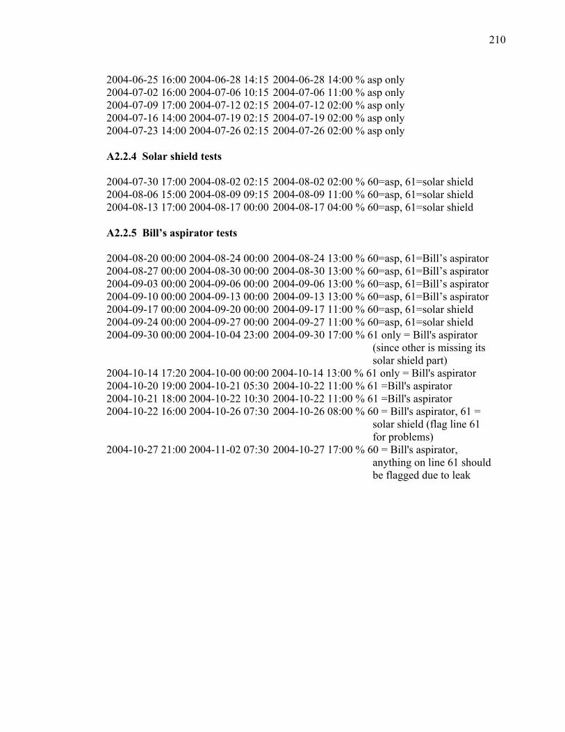
210
2004-06-25 16:00 2004-06-28 14:15 2004-06-28 14:00 % asp only 2004-07-02 16:00 2004-07-06 10:15 2004-07-06 11:00 % asp only 2004-07-09 17:00 2004-07-12 02:15 2004-07-12 02:00 % asp only 2004-07-16 14:00 2004-07-19 02:15 2004-07-19 02:00 % asp only 2004-07-23 14:00 2004-07-26 02:15 2004-07-26 02:00 % asp only A2.2.4 Solar shield tests 2004-07-30 17:00 2004-08-02 02:15 2004-08-02 02:00 % 60=asp, 61=solar shield 2004-08-06 15:00 2004-08-09 09:15 2004-08-09 11:00 % 60=asp, 61=solar shield 2004-08-13 17:00 2004-08-17 00:00 2004-08-17 04:00 % 60=asp, 61=solar shield A2.2.5 Bill’s aspirator tests 2004-08-20 00:00 2004-08-24 00:00 2004-08-24 13:00 % 60=asp, 61=Bill’s aspirator 2004-08-27 00:00 2004-08-30 00:00 2004-08-30 13:00 % 60=asp, 61=Bill’s aspirator 2004-09-03 00:00 2004-09-06 00:00 2004-09-06 13:00 % 60=asp, 61=Bill’s aspirator 2004-09-10 00:00 2004-09-13 00:00 2004-09-13 13:00 % 60=asp, 61=Bill’s aspirator 2004-09-17 00:00 2004-09-20 00:00 2004-09-17 11:00 % 60=asp, 61=solar shield 2004-09-24 00:00 2004-09-27 00:00 2004-09-27 11:00 % 60=asp, 61=solar shield 2004-09-30 00:00 2004-10-04 23:00 2004-09-30 17:00 % 61 only = Bill's aspirator
(since other is missing its solar shield part)
2004-10-14 17:20 2004-10-00 00:00 2004-10-14 13:00 % 61 only = Bill's aspirator 2004-10-20 19:00 2004-10-21 05:30 2004-10-22 11:00 % 61 =Bill's aspirator 2004-10-21 18:00 2004-10-22 10:30 2004-10-22 11:00 % 61 =Bill's aspirator 2004-10-22 16:00 2004-10-26 07:30 2004-10-26 08:00 % 60 = Bill's aspirator, 61 =
solar shield (flag line 61 for problems)
2004-10-27 21:00 2004-11-02 07:30 2004-10-27 17:00 % 60 = Bill's aspirator, anything on line 61 should be flagged due to leak