.

Continuous-Time Pension-Fund Modelling

Andrew J.G. Cairns 1 2

Department of Actuarial Mathematics and Statistics,Heriot-Watt University,

Riccarton, Edinburgh, EH14 4AS,United Kingdom

Abstract

This paper considers stochastic pension fund models which evolve in continuoustime and with continuous adjustments to the contribution rate and to the asset mix.A generalization of constant proportion portfolio insurance is considered and an an-alytical solution is derived for the stationary distribution of the funding level. In thecase where a risk-free asset exists this is a translated-inverse-gamma distribution.

Numerical examples show that the continuous-time model gives a very good ap-proximation to more widely used discrete time models, with, say, annual contribu-tion rate reviews, and using a variety of models for stochastic investment returns.

Keywords: continuous time; stochastic differential equation; risk-free rate; contin-uous proportion portfolio insurance.

1E-mail: A.Cairns@ma.hw.ac.uk2WWW: http://www.ma.hw.ac.uk/ andrewc/

1 Introduction

In this paper we consider continuous time stochastic models for pension fund dy-namics. The general form of this simple model is:

dXt Xtd t Xt N D Xt B dt

where Xt funding level at time t

Assets/Liabilities at time t

d t Xt real return between t and t dt

over salary growth

N normal contribution rate

D t Xt adjustment to the contribution rate

for surplus or deficit

and B rate of benefit outgo (as a proportion

of the actuarial liability)

(Note that the description of the model given here allows for the distribution ofinvestment returns to depend upon the funding level.)

Here, it is assumed that the level of benefit outgo is constant through time relativeto the actuarial liability.

Related to the funding level is the target funding level, L, which will normally beequal to 1 but this need not be the case. This reserve is related to the normal contri-bution rate, the level of benefit outgo and the valuation rate of interest in excess ofsalary growth, v, in the following way:

dLdt vL N B 0

That is, if the experience of the fund is precisely as expected then interest on thefund plus the normal contribution rate will be precisely sufficient to pay the benefits.Thus B N vL.

Similar continuous time models have been considered by Dufresne (1990). A dis-crete time version version of the model has been considered in more detail andin various forms by Cairns and Parker (1996), Dufresne (1988, 1989, 1990) andHaberman (1992, 1994).

This paper will discuss various special cases of the model. The first case is whered t Xt does not depend upon Xt and, in effect, reflects a static investment pol-

icy with independent and identically distributed returns. This case has previouslybeen considered by Dufresne (1990) who showed that the stationary distributionof the fund size was Inverse Gaussian and here we verify his result using differenttechniques.

The second case will consider Continuous Proportion Portfolio Insurance. This is aspecial type of investment strategy which holds a greater proportion of its assets inlow risk stocks when the funding level Xt is low. Several sub-cases are investigatedincluding one in which a risk-free asset exists and one in which it does not. Thelatter indicates that selling a particular asset class short could be a problem and as aconsequence certain constraints are put in place. These constraints prevent the fundfrom going short on the higher risk assets when the funding level is low and placean upper limit on the amount by which the fund can go short on low risk assetswhen the funding level is high. In all cases, a closed form solution can be found forthe limiting (stationary) density function of Xt . When there exists a risk-free asset,this distribution is Translated-Inverse-Gaussian (TIG).

Much of the analysis relies on the following result:

Theorem 1.1

Let the continuous-time stochastic process Xt satisfy the stochastic differential equa-tion

dXt Xt X2t

1 2dZt t Xtdt

subject to the constraints on the parameters 0, 0, 2 4 0, 0 and0.

(a) If 2 4 0, the stationary density function of Xt is

fX x k exp 2a tan 1 x bc

x x2 1

for x

where a1

4 22

b2

c4 2

2

where k is a normalizing constant.

(b) If 2 4 0 and X0 b, the stationary density function of Xt is

fX x k x b exp x b for b x

where b2

2 1

22

that is, the Translated-Inverse-Gamma distribution with parameters b, 1 0and 0 (T IG b 1 ). (If X TIG k then X k 1 Gamma .)

Proof See Cairns (1996).

2 Model 1: Static investment strategy

This model takes the simplest case possible. In the absence of other cashflows thevalue of the assets will follow Geometric Brownian motion. Thus

d t Xt d t dt dZt

where Zt is standard Brownian Motion.

In particular investment returns are uncorrelated and do not depend upon the fund-ing level at any point in time. Such a model is appropriate if the trustees of the fundoperate a static asset allocation strategy: that is, the proportion of the fund investedin each asset class remains fixed.

The deficit at time t is L Xt and the adjustment for this deficit to the contributionrate is

D Xt k L Xt

k 1 am is the spread factor, and m is the term of amortization.

This method is sometimes referred to as the spread method of amortization (forexample, see Dufresne, 1988).

In continuous time this model has been considered by Dufresne (1990).

The stochastic differential equation for the fund size is

dXt dt dZt Xt N B k L Xt dt Xtdt XtdZt t

where k and k v L.

2.1 Properties of X

Let X be a random variable with the stationary distribution of Xt . (Cairns and Parker,1996, show that such processes are stationary and ergodic.)

Now Xt falls into the collection of stochastic processes covered in Theorem 1.1 Thusby Theorem 1.1(b) X has an Inverse Gamma distribution with parameters 1 and

where 2 1 2 and 2 2

4 (that is, X 1 Gamma 1 ). For this

to be a proper distribution (that is, one which has a density which integrates to 1)we require that 1. This therefore imposes the further condition that k 1

22.

Stronger conditions on k are required to ensure that X has finite moments.

The stationary distribution of Xt was found by Dufresne (1990), Proposition 4.4.4,but here we have derived it in a different way by making use of Theorem 1.1.

Let M j E X j where j is a non-negative integer. Then it is easy to show that forj 1

M j

j

2 3 j 1

For j 1, M j is infinite.

Using these equations we see that

E Xk v

kL

E X2 k v2

k k 12

2L2

Var Xk v

2 12

2

k 2 k 12

2L2

Note that it is possible for the process to be stationary but to have an infinite mean.

Using this information we can calculate, for example, Pr X x0 where x0 is thegovernment statutory limit of 105% of the actuarial liability calculated on the UKstatutory valuation basis. This figure gives a guide to the frequency in the long runof breaches of this upper limit.

2.2 Hitting Times

The problems described below are included as open problems.

Suppose T inf t : Xt x . Since Xt is stationary it cannot be true that E s XT

E s X0 . If, on the other hand, 0 x X0 y and T inf t : Xt x or y thenE s XT s x Pr XT x s y Pr XT y E s X0 .) Since no closed formfor s x exists this problem must be solved numerically.

The problem can be generalized to allow us to gain further information about astopping time T . Suppose we are interested in the first time, T , that the process Xt

reaches some level x or hits an upper or a lower bound (y or x). We can at least inprinciple obtain the moment generating function for T by generalizing the approachdescribed in Section 2.1.

Let Yt f t Xt F t G Xt , which we wish to be a martingale.

Then by Ito’s formula we have

dY FGdt FG dX12

FG dX 2

FG XdZ FG12

2X2FG XFG G dt

For Yt to be a martingale we therefore require the dt term to be equal to zero. Thatis

F tF t

1G x

2x2

2G x x G x

F t F0 exp t

and G x satisfies:

x2G x x G x G x 0

where 2 2, 2 2 and 2 2.

Again, no general form for G x can be found, so numerical solutions seems toprovide the way forward. However, it may be possible to prove qualitative resultsregarding the shape of the distribution of T .

3 Model 2: Continuous Proportion Portfolio Insur-ance

Black and Jones (1988) and Black and Perold (1992) discuss an investment strategycalled Continuous Proportion Portfolio Insurance (CPPI) which is appropriate forfunds which have some sort of minimum funding constraint imposed by either bylaw or by the trustees of the fund.

When the funding level is low (A L M) all assets should be invested in a low riskportfolio (relative to the M). As A L rises above M any surplus and, perhaps more,should be invested in higher risk assets.

This is in contrast to the static investment strategy discussed in Section 2 whichrebalances the portfolio continuously to retain the same proportion of assets in eachasset class.

Suppose that we have two assets in which we can invest. Asset 1 is risk free andoffers an instantaneous rate of return of 1. Asset 2 is a risky asset with d 2 t

2dt 2dZt . 1 2 and 22 0 (with 2

2 0). Since asset 2 is risky we have2 1.

Let p t be the proportion of assets at time t which are invested in asset 2 and letXt be the funding level at time t. Under the static investment strategy p t p forall t. Under the CPPI strategy p t depends on Xt only: p t 0 whenever Xt M;and p t p Xt 0 when Xt M. A strategy which results in p t 1 for somevalues of Xt allows for the risk-free asset to be sold short.

We consider the case p t Xt M Xt . Then

dXt p t Xtd 2 t 1 p t Xt 1dt k v Ldt kXtdt

Xt M 2dt 2dZt M 1dt k v Ldt

k Xt M dt kMdt

Hence

d Xt M c dt a Xt M dt 2 Xt M dZt

where a k 2

c k v L k 1 M

Xt M Inverse-Gamma 1

where 2 1a22

2c22

E Xt M2

Var Xt M2

2 2 3

Therefore we have

E Xt Mk v L k 1 M

k 2

Var Xtk v L k 1 M

k 2

2 22

2 k 222

provided k 212

22

From these equations, we see that we require c 0 to ensure that Xt M for allt almost surely (that is, the risk-free interest plus the amortization effort must besufficient to keep the funding level above M). We also require a 0 (that is, k 2)to ensure that Xt does not tend to infinity almost surely. Finally we can see that thevariance will be infinite if k 2

12

22.

4 Comparing models 1 and 2

Models 1 and 2 describe two quite different asset allocation strategies and it is,therefore, useful to be able to compare them and to decide which strategy is betterand when. The following theorem answers this to a certain extent.

Theorem 4.1

Suppose that we have a risk-free asset (with d 1 t 1 dt) and a risky asset (withd 2 t 2 dt 2dZ t ).

Under CPPI the mean funding level is E Xt and its variance is 2C Var Xt .

Under a static investment strategy we invest a proportion p is the risky asset and1 p in the risk-free asset.

There exists p such that under the static investment strategy E Xt (as withCPPI) and Var Xt

2S

2C.

Proof See Cairns (1996) but note that the appropriate value of p is M .

Interpretation: In the variance sense, the static strategy is more efficient than CPPI:that is, given a CPPI strategy we can always find a static strategy which delivers thesame mean funding level but a lower variance.

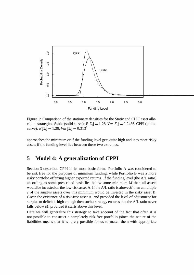
One example illustrating this result is plotted in Figure 1.

Under CPPI we have 1 0 02 2 0 05 v 0 015 22 0 152, L 1 M 0 7

and k 0 1. This gives rise to E Xt 1 28, Var Xt 0 3132. The mean is rela-tively high because the valuation rate of interest v appears very cautious. However,the use of such a cautious basis is not necessarily too far from regular practice.

Under the equivalent static strategy which has E Xt 1 28 we invest 45.3% of thefund in asset 2 and 54.7% of the fund in the risk-free asset 1. The stationary varianceof the fund size is then found to be Var Xt 0 2432.

The static variance is significantly less than that for CPPI. This is not too evidentfrom Figure 1, but arises out of the fact that the CPPI density has a much fatter righthand tail. CPPI also gives a much more skewed distribution.

Now there are various reasons for why we may prefer CPPI to the static strategy.Principally this will happen when the objective of the pension fund is more thanjust to minimize the variance of the contribution rate. For example, there may bea penalty attached to a funding level which is below some minimum. In the exam-ple above, if this is anything below about 0.9 then CPPI may be favoured. Moregenerally some utility functions may result in a higher expected utility for CPPI (inparticular, those which penalize low funding levels).

Conversely there exist utility functions which result in optimal strategies whichare the exact opposite of CPPI. For example, Boulier et al. (1995) maximize thefunction

V0

exp s C t 2ds

where C t N D t Xt is the contribution rate at time t.

They found that the optimal strategy was to invest in risky assets when the fundinglevel is low and to move into toe risk-free asset as the funding level increases. Therationale behind this is that if there is no minimum funding constraint then: (a) oneshould try to reach a high funding level as quickly as possible, no matter how riskythe strategy; and (b) when a high funding position is reached then this should beprotected. Investing in a low risk strategy when the funding level is high will dotwo things: (a) protect the low contribution rate; and (b) reduce the risk that if toomuch surplus is generated then the benefits will have to be improved.

In practice, one may wish to combine these two extremes by having a bell shapedasset allocation: that is, one which moves into the risk-free asset if the funding level

0.0 0.5 1.0 1.5 2.0 2.5 3.0

0.0

0.5

1.0

1.5

2.0

Funding Level

Pro

babi

lity

Den

sity

Static

CPPI

Figure 1: Comparison of the stationary densities for the Static and CPPI asset allo-cation strategies. Static (solid curve): E Xt 1 28, Var Xt 0 2432. CPPI (dottedcurve): E Xt 1 28, Var Xt 0 3132.

approaches the minimum or if the funding level gets quite high and into more riskyassets if the funding level lies between these two extremes.

5 Model 4: A generalization of CPPI

Section 3 described CPPI in its most basic form. Portfolio A was considered tobe risk free for the purposes of minimum funding, while Portfolio B was a morerisky portfolio offerring higher expected returns. If the funding level (the A/L ratio)according to some prescribed basis lies below some minimum M then all assetswould be invested on the low-risk asset A. If the A/L ratio is above M then a multiplec of the surplus assets over this minimum would be invested in the risky asset B.Given the existence of a risk-free asset A, and provided the level of adjustment forsurplus or deficit is high enough then such a strategy ensures that the A/L ratio neverfalls below M, provided it starts above this level.

Here we will generalize this strategy to take account of the fact that often it isnot possible to construct a completely risk-free portfolio (since the nature of theliabilities means that it is rarely possible for us to match them with appropriate

assets).

Suppose that we may invest in a range of n assets. The values of these assets allfollow correlated Geometric Brownian Motion. Thus asset j produces a return inthe time interval [t, t+dt) of

d j t jdtn

k 1

c jkdZk t

where Z1 t Zn t are independent standard Brownian Motions.

At all times portfolio A invests a proportion Aj in asset j for j 1 2 n, with

the portfolio being continually rebalanced to ensure that the proportions invested ineach asset remain constant.

Portfolio B follows the same strategy but has a different balance of assets Bj

nj 1.

Portfolio B invests in what may be regarded as more risky assets than does portfolioA.

For portfolio A the return in the time interval [t, t+dt) is

d A tn

j 1

Aj jdt

n

k 1

c jkdZk t

similarly for portfolio B the return in the time interval [t, t+dt) is

d B tn

j 1

Bj jdt

n

k 1

c jkdZk t

The matrix C c jk is somewhat arbitrary but has the constraint that CCT Vwhere V is the symmetric convariance matrix for the n assets.

These equations can be condensed into the following forms:

d A t Adt AAdZA t ABdZB t

d B t Bdt BAdZA t BBdZB t

where A

n

j 1

Aj j

B

n

j 1

Bj j

and if S AA AB

BA BB

then SSTTAV A

TAV B

TBV A

TBV B

Thus without loss of generality we may work with two assets 1 and 2 instead of thetwo portfolios A and B.

At any time a proportion of the fund p t is invested in asset 2. Thus the return inthe time interval [t, t+dt) is

d t 1 p t d 1 t p t d 2 t

where d 1 t 1dt 11dZ1 t 12dZ2 t

d 2 t 2dt 21dZ1 t 22dZ2 t

In a continuous time stationary pension fund model there is a continuous inflowof contribution income C t and a continuous outflow of benefit payments B. Thecontribution rate is made up of two parts: the normal contribution rate N; and anadjustment for the difference between the funding level X t and the target level ofL. Thus C t N k L X t .

The stochastic differential equation governing the dynamics of the fund size is there-fore

dX t X t d t N B k L X t dt

Note that if v is the valuation force of interest then N, B and L are related by thebalance equation 0 dL vLdt N B dt which implies that N B vL.Hence

dX t X t d t k v L kX t dt

Generalizing the formulation of Black and Jones (1988) we suppose that

p tp0 p1X t

X t

Then (abbreviating X t by X and dX t by dX etc.) we have

dX p0 1 p1 X 1dt 11dZ1 12dZ2

p0 p1X 2dt 21dZ1 22dZ2

kXdt k v Ldt

p0 21 11 1 p1 11 p1 21 X dZ1

p0 22 12 1 p1 12 p1 22 X dZ2

p0 2 1 k v L dt

1 p1 1 p1 2 k X dt

X X2 1 2dZ3 t Xdt

where Z3 t is a standard Brownian Motion and

p20 21 11

222 12

2

2p0 21 11 1 p1 11 p1 21

22 12 1 p1 12 p1 22

1 p1 11 p1 212 1 p1 12 p1 22

2

p0 2 1 k v L

k 1 p1 1 p1 2

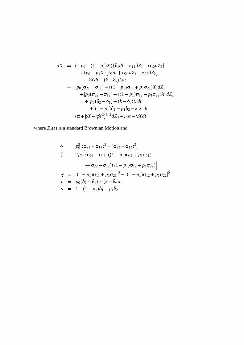
This stochastic differential equation for X t is therefore in the correct form forTheorem 1.1. Thus the stationary distribution of X t is

fX x k exp 2a tan 1 x bc

x x2 1

for x

where a1

4 22

b2

c4 2

2

This is true provided that it is not possible to synthesize a risk-free asset out of thetwo portfolios. If that is the case then we will have 4 2 0.

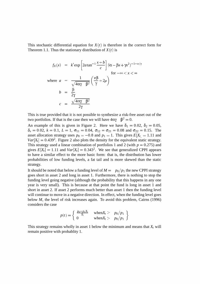
An example of this is given in Figure 2. Here we have 1 0 02, 2 0 05,v 0 02, k 0 1, L 1, 11 0 04, 12 21 0 08 and 22 0 15. The

asset allocation strategy uses p0 0 8 and p1 1. This gives E Xt 1 11 andVar Xt 0 4392. Figure 2 also plots the density for the equivalent static strategy.This strategy used a linear combination of portfolios 1 and 2 (with p 0 275) andgives E Xt 1 11 and Var Xt 0 3432. We see that generalized CPPI appearsto have a similar effect to the more basic form: that is, the distribution has lowerprobabilities of low funding levels, a fat tail and is more skewed than the staticstrategy.

It should be noted that below a funding level of M p0 p1 the new CPPI strategygoes short in asset 2 and long in asset 1. Furthermore, there is nothing to stop thefunding level going negative (although the probability that this happens in any oneyear is very small). This is because at that point the fund is long in asset 1 andshort in asset 2. If asset 2 performs much better than asset 1 then the funding levelwill continue to move in a negative direction. In effect, when the funding level goesbelow M, the level of risk increases again. To avoid this problem, Cairns (1996)considers the case

p tp0 p1Xt

XtwhenXt p0 p1

0 whenXt p0 p1

This strategy remains wholly in asset 1 below the minimum and means that Xt willremain positive with probablity 1.

0.0 0.5 1.0 1.5 2.0 2.5 3.0

0.0

0.5

1.0

1.5

Static

Gen.CPPI

Funding Level

Pro

babi

lity

Den

sity

Figure 2: Comparison of the stationary densities for the Static and GeneralizedCPPI asset allocation strategies. Static (solid curve): E Xt 1 11, Var Xt

0 3432. Generalized CPPI (dotted curve): E Xt 1 11, Var Xt 0 4392.

6 References

Black, F. and Jones, R. (1988) Simplifying portfolio insurance for corporate pen-sion plans. Journal of Portfolio Management 14(4), 33-37.

Black, F. and Perold, A. (1992) Theory of constant proportion portfolio insurance.Journal of Economic Dynamics and Control 16, 403-426.

Boulier, J-F., Trussant, E. and Florens, D. (1995) A dynamic model for pensionfunds management. Proceedings of the 5th AFIR International Colloquium 1,361-384.

Cairns, A.J.G. (1996) Continuous-time stochastic pension fund models. In prepa-ration.

Cairns, A.J.G. and Parker, G. (1996) Stochastic pension fund modelling. Submit-ted.

Dufresne, D. (1988) Moments of pension contributions and fund levels when ratesof return are random. Journal of the Institute of Actuaries 115, 535-544.

Dufresne, D. (1989) Stability of pension systems when rates of return are random.Insurance: Mathematics and Economics 8, 71-76.

Dufresne, D. (1990) The distribution of a perpetuity, with applications to risktheory and pension funding. Scandinavian Actuarial Journal 1990, 39-79.

Haberman, S. (1992) Pension funding with time delays: a stochastic approach.Insurance: Mathematics and Economics 11, 179-189.

Haberman, S. (1994) Autoregressive rates of return and the variability of pensionfund contributions and fund levels for a defined benefit pension scheme. Insurance:Mathematics and Economics 14, 219-240.

Oksendal, B. (1992) Stochastic Differential Equations. Springer Verlag, Berlin.

Parker, G. (1994) Limiting distribution of the present value of a portfolio of poli-cies. ASTIN Bulletin 24, 47-60.