Control System Designibruce/courses/old_ee... · Chapter 6 ©Goodwin, Graebe, Salgado, Prentice Hall 2000 Different PID Structures? A key issue when applying PID tuning rules (such

ELEC ENG 4CL4:

Control System Design

Notes for Lecture #12Friday, January 31, 2003

Dr. Ian C. BruceRoom: CRL-229Phone ext.: 26984Email: [email protected]

©Goodwin, Graebe, Salgado, Prentice Hall 2000Chapter 6

Tuning of PID Controllers

Because of their widespread use in practice, wepresent below several methods for tuning PIDcontrollers. Actually these methods are quite old anddate back to the 1950’s. Nonetheless, they remain inwidespread use today.In particular, we will study.

◆ Ziegler-Nichols Oscillation Method◆ Ziegler-Nichols Reaction Curve Method◆ Cohen-Coon Reaction Curve Method


(1) Ziegler-Nichols (Z-N) Oscillation Method

This procedure is only valid for open loop stableplants and it is carried out through the followingsteps

◆ Set the true plant under proportional control, with avery small gain.

◆ Increase the gain until the loop starts oscillating. Notethat linear oscillation is required and that it should bedetected at the controller output.


◆ Record the controller critical gain Kp = Kc and theoscillation period of the controller output, Pc.

◆ Adjust the controller parameters according to Table6.1 (next slide); there is some controversy regardingthe PID parameterization for which the Z-N methodwas developed, but the version described here is, to thebest knowledge of the authors, applicable to theparameterization of standard form PID.


Table 6.1: Ziegler-Nichols tuning using theoscillation method

Kp Tr Td

P 0.50Kc

PI 0.45KcPc

1.2PID 0.60Kc 0.5Pc

Pc

8


General System

If we consider a general plant of the form:

then one can obtain the PID settings via Ziegler-Nichols tuning for different values of τ and ν0. Thenext plot shows the resultant closed loop stepresponses as a function of the ratio

0;1)( 000

0 >+=−

γγτ

seKsG

s

.0ν

τ∆=x


Figure 6.3: PI Z-N tuned (oscillation method) controlloop for different values of the ratio .

00

ντ∆

=x

0 1 2 3 4 5 6 7 8 9 100

0.5

1

1.5

Time [t/τ]

Pla

nt r

espo

nse

Ziegler−Nichols (oscillation method) for different values of the ratio x= τ/νo

x=0.1

x=0.5

x=2.0


Numerical Example

Consider a plant with a model given by

Find the parameters of a PID controller using theZ-N oscillation method. Obtain a graph of theresponse to a unit step input reference and to a unitstep input disturbance.

Go(s) =1

(s + 1)3


Solution

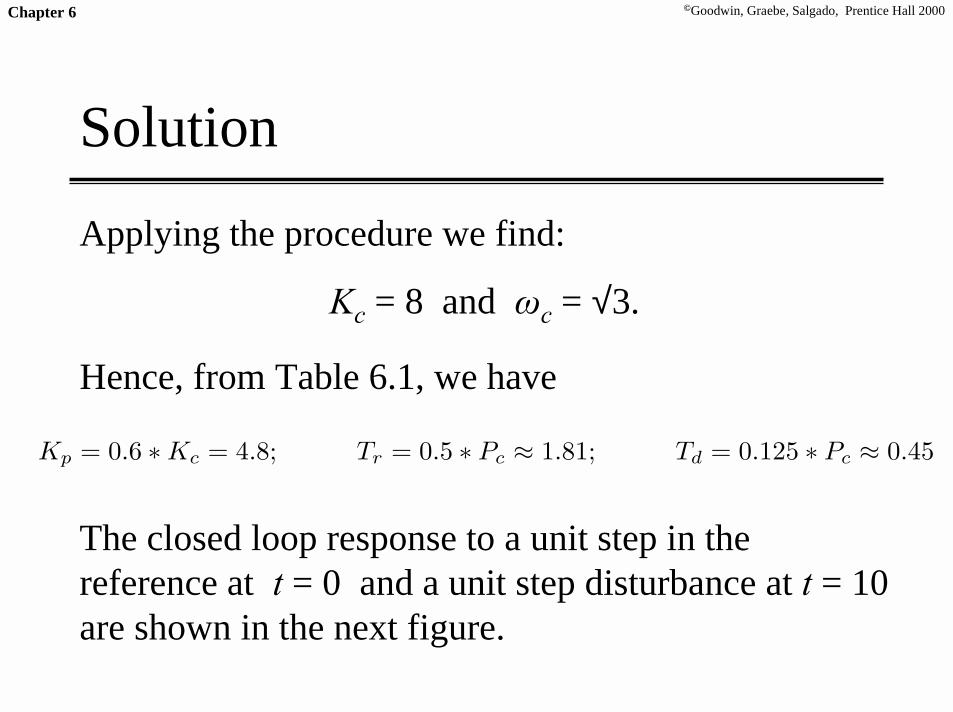
Applying the procedure we find:

Kc = 8 and ωc = √3.

Hence, from Table 6.1, we have

The closed loop response to a unit step in thereference at t = 0 and a unit step disturbance at t = 10are shown in the next figure.

Kp = 0.6 ∗ Kc = 4.8; Tr = 0.5 ∗ Pc ≈ 1.81; Td = 0.125 ∗ Pc ≈ 0.45


Figure 6.4: Response to step reference and stepinput disturbance

0 2 4 6 8 10 12 14 16 18 200

0.5

1

1.5

Time [s]

Pla

nt o

utpu

t

PID control tuned with Z−N (oscillation method)


Different PID Structures?

A key issue when applying PID tuning rules (such asZiegler-Nichols settings) is that of which PIDstructure these settings are applied to.To obtain an appreciation of these differences weevaluate the PID control loop for the same plant inExample 6.1, but with the Z-N settings applied to theseries structure, i.e. in the notation used in (6.2.5),we have

Ks = 4.8 Is = 1.81 Ds = 0.45 γs = 0.1


Figure 6.5: PID Z-N settings applied to seriesstructure (thick line) and conventionalstructure (thin line)

0 2 4 6 8 10 12 14 16 18 200

0.5

1

1.5

2

Time [s]

Pla

nt o

utpu

t

Z−N tuning (oscillation method) with different PID structures


Observation

In the above example, it has not made muchdifference, to which form of PID the tuning rules areapplied. However, the reader is warned that this canmake a difference in general.


(2) Reaction Curve Based Methods

A linearized quantitative version of a simple plantcan be obtained with an open loop experiment, usingthe following procedure:

1. With the plant in open loop, take the plant manually to anormal operating point. Say that the plant output settles aty(t) = y0 for a constant plant input u(t) = u0.

2. At an initial time, t0, apply a step change to the plantinput, from u0 to u∞ (this should be in the range of 10 to20% of full scale).

Cont/...


3. Record the plant output until it settles to the new operatingpoint. Assume you obtain the curve shown on the nextslide. This curve is known as the process reaction curve.

In Figure 6.6, m.s.t. stands for maximum slope tangent.

4. Compute the parameter model as follows

Ko =y∞ − yo

u∞ − uo; τo = t1 − to; νo = t2 − t1


Figure 6.6: Plant step response

The suggested parameters are shown in Table 6.2.

Time (sec.)

y∞

yo

to t

1 t

2

m.s.t.


Table 6.2: Ziegler-Nichols tuning using the reactioncurve

Kp Tr Td

Pνo

Koτo

PI0.9νo

Koτo3τo

PID1.2νo

Koτo2τo 0.5τo


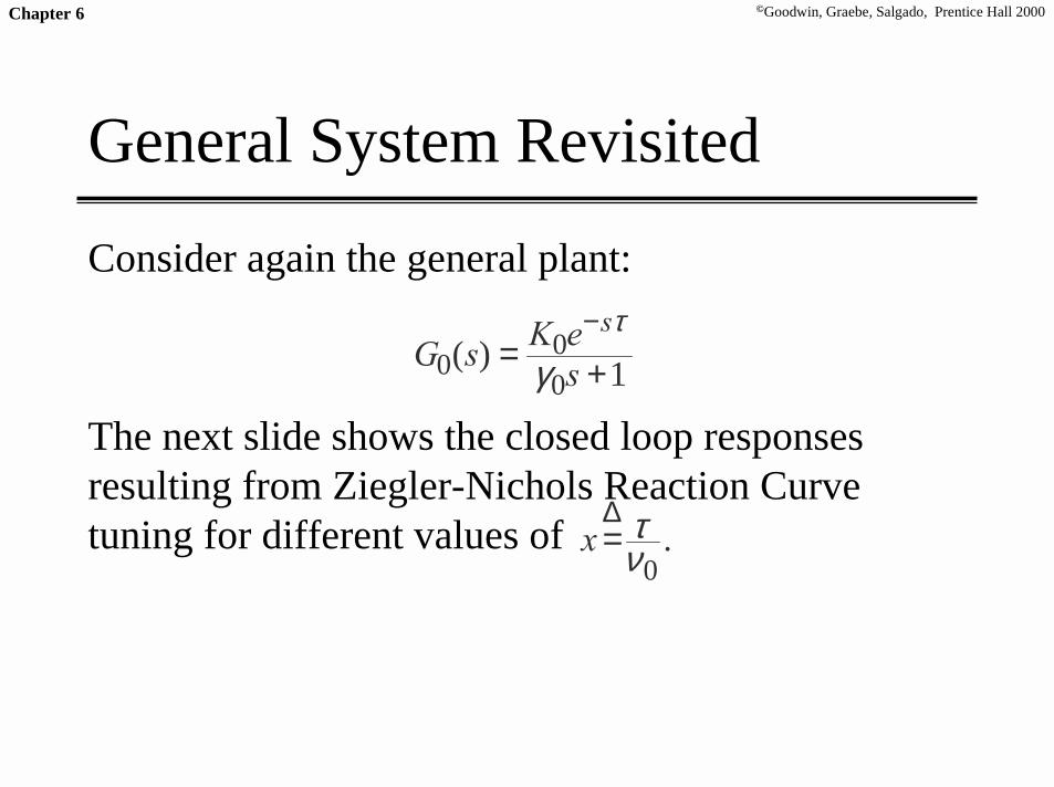
General System Revisited

Consider again the general plant:

The next slide shows the closed loop responsesresulting from Ziegler-Nichols Reaction Curvetuning for different values of

1)(00

0 +=−

seKsG

s

γτ

.0ν

τ∆=x


Figure 6.7: PI Z-N tuned (reaction curve method)control loop

0 5 10 150

0.5

1

1.5

2

Time [t/τ]

Pla

nt r

espo

nse

Ziegler−Nichols (reaction curve) for different values of the ratio x= τ/νo

x=0.1

x=0.5

x=2.0


Observation

We see from the previous slide that the Ziegler-Nichols reaction curve tuning method is verysensitive to the ratio of delay to time constant.

Documents

Control System Designibruce/courses/old_ee... · Chapter 6 ©Goodwin, Graebe, Salgado, Prentice Hall 2000 Different PID Structures? A key issue when applying PID tuning rules (such