Embed Size (px)
Citation preview
PROBABILITY TUTORIALSwww.probability.net
Convexity Adjustment betweenFutures and Forward Rate Using a
Martingale Approach
N. Vaillant
Directory
• Table of Contents.• Begin Article.
Copyright c© 1999 [email protected] Revision Date: December 2, 1999 Version 2.0

Table of Contents
1. Introduction2. Theoretical derivation
2.1. The underlying principle2.2. Valuing a FRA using futures2.3. The convexity adjustment
3. Practical Results3.1. Approximating the convexity adjustment3.2. Spreadsheet implementation for Eurodollars3.3. Conclusion
A. appendixB. appendixC. appendixD. appendix
Section 1: Introduction 3
1. IntroductionThe purpose of this report is to describe the question of the convexityadjustment needed to convert a forward rate to its corresponding fu-tures rate. Because of the marking to market of any profit and loss ona futures position, strictly speaking futures and forward contracts donot provide equal payoffs. It is therefore not surprising that futuresand forward rates should be different.
The theoretical results presented in this report are due to PaulDoust [1]. However, we shall resort to a slightly different approach,making use of martingales as opposed to PDE’s, and making smalladjustments to distributional assumptions. It is reassuring to seethat whichever way one looks at it, the same convexity adjustment isobtained.
This report can be divided in two parts. We shall first derive atheoretical formula for the convexity adjustment. A second part willshow how to approximate such formula, and provide comments on theresults obtained, after a simple spreadsheet implementation.
Section 2: Theoretical derivation 4
2. Theoretical derivation
2.1. The underlying principle
Let T and T + ∆T be the starting and end dates of a forward period.We denote Lt the forward rate between T and T + ∆T at time t,and Ft the futures rate at time t corresponding to the same period.Note that both rates Lt and Ft will converge at time T to the thenprevailing money market rate with maturity ∆T , so that LT = FT .
Let Vt denote the T + ∆T discount factor at time t. A forwardcontract struck at a rate K is a contingent claim with final payoff attime T equal to:
ΠT = αVT (LT −K) (1)
where α denotes the day count fraction between T and T + ∆T .The value today (t = 0) of such a forward contract is given by:
Π0 = αV0(L0 −K) (2)
and as we can see, this value is a function of the current discount
Section 2: Theoretical derivation 5
factor V0 and forward rate L0. However, since LT = FT , the finalpayoff ΠT could also have been written as:
ΠT = αVT (FT −K) (3)
This important point, together with the fact that futures contractscan actually be traded, will enable to show that the current value Π0
of our forward contract is also a function of V0 and the current futuresrate F0, i.e.
Π0 = f(V0, F0) (4)
for some appropriate function f . It can therefore be seen from (2)and (4) that the current forward rate L0 and its corresponding futuresrate F0 are linked together by:
αV0(L0 −K) = f(V0, F0) (5)
In general, the function f is not given by αV0(F0 − K), and L0 isnot equal to F0. Determining the explicit form of the function f willenable us through (5), to determine the exact link between F0 andL0, which is the so called convexity adjustment.
Section 2: Theoretical derivation 6
2.2. Valuing a FRA using futures
Determining f(V0, F0) amounts to valuing a forward contract viewedas a contingent claim with final payoff (3). In order to do that, weshall call v0 = f(V0, F0) the unknown premium to be determined. Weconsider an investor receiving an initial (t = 0) amount of cash equalto v0, and engaging in a continuous trading strategy θ = (θt) in thefutures contract,1 where all cash is reinvested in the discount bond Vt.If we call πt the value of the investor’s portfolio at time t, then theprocess π = (πt) is given by π0 = v0, and the stochastic differentialequation: 2
dπt = θtdFt +πtVtdVt (6)
1At time t, the investor has a long position θt in the rate Ft, which actuallycorresponds to a short position in terms of contracts.
2 Note that by writing (6), we have neglected the effect of minimum marginrequirements. In real life, an investor entering a futures contract could not reinvestthe totality of his profits in the discount bond, since some of his cash has to beleft on his margin account.
Section 2: Theoretical derivation 7
In other words, a variation dπt in the portfolio’s value arises due tovariations dFt and dVt, and the two long positions θt and πt/Vt in Ftand Vt respectively. The solution to (6), given the initial conditionπ0 = v0 , can be expressed as:3
πt = Vt
(v0
V0+∫ t
0
θtdFt
)(7)
where:Ft4= Ft/Ct (8)
θt4= θtCt/Vt (9)
and the process C = (Ct) has been defined as:
Ct4= exp
(∫ t
0
1FsVs
d〈F, V 〉s)
(10)
3See appendix A.
Section 2: Theoretical derivation 8
In particular, our investor will have a final wealth at time T equal to:
πT = πT (v0, θ) = VT
(v0
V0+∫ T
0
θtdFt
)(11)
This final wealth is obviously a function of the initial premium v0 andtrading strategy θ. Now, suppose for a moment that we could find v0
and θ such that:πT (v0, θ) = αVT (FT −K) (12)
Then, an investor receiving an initial cash payment of v0 and enteringthe strategy θ, will exactly generate a final wealth equal to the finalpayoff of our forward contract. In other words, an initial investmenttogether with adequate trading, enables the exact replication of aforward contract payoff. To avoid any possibility of arbitrage, thevalue of this forward contract has to be the initial investment v0.Hence, if we can find v0 and θ satisfying (12), then we know that v0
is exactly the premium that we are looking for.
Section 2: Theoretical derivation 9
Our problem of finding v0 can now be rephrased in terms of thefollowing questions:
1. Do there exist v0 and θ such that (12) holds?
2. If so, how do we calculate v0?
Of course, the answer to these questions will very much depend on theparticular assumptions made on the processes V = (Vt) and F = (Ft).In general, it is not true that v0 and θ always exist, and if they do, ac-tually computing v0 can be quite tedious. However, without (for now)being more specific on V and F , we can indicate the general procedureenabling to get answers to the above questions: firstly, comparing (12)with (11) shows that v0 and θ should satisfy the equation:
v0
V0+∫ T
0
θtdFt = α(FT −K) (13)
Now, let us assume that there exists a probability measure Q, un-
Section 2: Theoretical derivation 10
der which the process F = (Ft) (as defined in (8) ) is a martingale,4
and furthermore, that the martingale representation theorem can ac-tually be applied:5 this theorem states the existence of a constant x0
together with a process φ = (φt) such that:
x0 +∫ T
0
φtdFt = α(FT −K) (14)
Of course, we do not know explicitly what x0 and φ are. But we areonly interested in their existence: for once we know that x0 and φ doexist, then defining v0
4= x0V0 and θt
4= Vtφt/Ct, equation (14) can
be rewritten as (13), which shows the existence of a premium v0 anda strategy θ satisfying equation (12). This is the answer to the abovefirst question.
4See appendix C for the proof of such existence, (provided we make the rightassumptions). Do not be put off by the terminology here: everything you need toknow is recalled below.
5See appendix D for the proof of that.
Section 2: Theoretical derivation 11
Having answered question 1, we are now left with the task ofactually computing v0. As we shall see, there is very little to it:indeed, the nice thing about F = (Ft) being a martingale under Q, isthat we can always write:6
EQ
[∫ T
0
θtdFt
]= 0 (15)
and taking Q-expectation on both sides of (13), we therefore obtain:
v0 = αV0(EQ[FT ]−K) (16)
which shows that computing v0 amounts to the computation of theQ-expectation EQ[FT ]. In general, this expectation can be quite dif-ficult to obtain explicitly. However, if the assumptions made on theprocesses F and V are such that the process C = (Ct) as defined
6We are being slightly over optimistic here. In reality, some integrability con-dition has to be met by θ. See appendix D.
Section 2: Theoretical derivation 12
in (10) is actually deterministic,7 then we have the following:8
EQ[FT ] = EQ[FTCT ] = CTEQ[FT ] = CTF0 (17)
which can be substituted into (16) in order to obtain:
f(V0, F0)4= v0 = αV0(CTF0 −K) (18)
This completes our task of answering questions 1 and 2. It should beremembered however, that before deriving anything like (18), someassumptions had to be made. In other words, taking just any kindof diffusion for the processes F and V will inevitably lead to thecollapse of the previous developments. When confronted with the
7 This looks like we have an additional requirement on F and V . In fact, theassumption of C being deterministic is also needed to ensure that the martingalerepresentation theorem can be applied. See appendix D
8 F being a martingale under Q, (and F0 being constant), EQ[FT ] = EQ[F0] =F0.
Section 2: Theoretical derivation 13
task of designing our financial model, three fundamental points haveto be kept in mind:9
1. We need a probability measure Q, under which F is a martin-gale.
2. The martingale representation theorem must be applicable.
3. The process C = (Ct) should be deterministic.
2.3. The convexity adjustment
In the previous section, we were able to explicitly determine f(V0, F0)by equation (18). Looking back at (5), it appears that the forwardrate L0 and futures rate F0 satisfy the equation:
αV0(L0 −K) = αV0(CTF0 −K) (19)
9As already mentioned, point 3 is in fact a prerequisite to point 2.
Section 2: Theoretical derivation 14
from which we conclude that:
L0 = CTF0 (20)
In other words, the forward rate L0 is equal to the futures rate F0
times a convexity adjustment CT given by:10
CT = exp
(∫ T
0
1FtVt
d〈F, V 〉t
)(21)
In order to give a more explicit formulation of CT , it is now timeto be more specific about the processes F = (Ft) and V = (Vt). Asdetailed in appendix B, the chosen diffusion for F and V are:
dFt = µ(t)Ftdt+ σF (t)FtdWt (22)
Vt4= exp(−(T + ∆T − t)Rt) (23)
10 There is no particular reason to call CT a convexity adjustment, apart fromcurrent practice.
Section 2: Theoretical derivation 15
dRt = γ(R∞ −Rt)dt+ σR(t)R∞dW ′′t (24)
with F0, R0 > 0, where γ,R∞ are strictly positive constants, and allprocesses µ, σF , σR are deterministic. It is of course understood thatW and W ′′ in (22) and (24) are standard brownian motions. Fur-thermore, we assume that W and W ′′ have deterministic correlationρ(t).
In appendix B, we show that given (22), (23) and (24), the con-vexity adjustment CT can be expressed as:11
CT = exp
(−R∞
∫ T
0
(T + ∆T − t)σR(t)σF (t)ρ(t)dt
)(25)
11 Paul Doust [1] assumes log-normal diffusion for both F and V , with deter-ministic correlation ρF,V . In this case we obtain:
CT = exp
Z T
0σV (t)σF (t)ρF,V (t)dt
Section 3: Practical Results 16
3. Practical Results
3.1. Approximating the convexity adjustment
In the previous section, we obtained formula (25), giving the convex-ity adjustment needed to convert a futures rate to its correspondingforward rate. As we can see, some additional assumptions have tobe made on σR(t) ,σF (t) and ρ(t) in order to compute the integralin (25) explicitly. Following Paul Doust in [2], we shall put:
∀t ∈ R+ , σR(t) = σF (t) = σ (26)
where σ is meant to represent some sort of average volatility for rates.This approximation could obviously be improved: it is widely ac-knowledged that volatilities for long rates are usually lower than shortterm volatilities. Hence, σR(t) could be chosen to be an increasingfunction of time. As we shall see, given (26), the sensitivity of theconvexity adjustment (25) with respect to the parameter σ (and in-deed w.r. to R∞), will not appear to be significant compared to the
Section 3: Practical Results 17
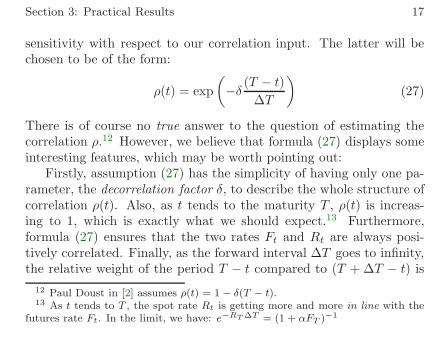
sensitivity with respect to our correlation input. The latter will bechosen to be of the form:
ρ(t) = exp(−δ (T − t)
∆T
)(27)
There is of course no true answer to the question of estimating thecorrelation ρ.12 However, we believe that formula (27) displays someinteresting features, which may be worth pointing out:
Firstly, assumption (27) has the simplicity of having only one pa-rameter, the decorrelation factor δ, to describe the whole structure ofcorrelation ρ(t). Also, as t tends to the maturity T , ρ(t) is increas-ing to 1, which is exactly what we should expect.13 Furthermore,formula (27) ensures that the two rates Ft and Rt are always posi-tively correlated. Finally, as the forward interval ∆T goes to infinity,the relative weight of the period T − t compared to (T + ∆T − t) is
12 Paul Doust in [2] assumes ρ(t) = 1− δ(T − t).13 As t tends to T , the spot rate Rt is getting more and more in line with the
futures rate Ft. In the limit, we have: e−RT∆T = (1 + αFT )−1
Section 3: Practical Results 18
t T+∆TT
: Continuously compounded spot rateR t
F t : Futures rates
T-t ∆T
Figure 1: ρ(t) = e−δ(T−t)/∆T is assumed to be the correlation betweenthe futures rate Ft and continuously compounded spot rate Rt.
Section 3: Practical Results 19
getting smaller and smaller. Hence, one would expect the correspond-ing correlation to increase to the value 1, as is indeed the case withformula (27).
Having made assumptions (26) and (27), the computation of theconvexity adjustment (25) is just a simple exercise. We obtain:
CT = exp[−σ
2R∞(∆T )2
δ2
((δ + 1)
(1− e−δT/∆T
)−(δT
∆T
)e−δT/∆T
)](28)
Note that in the limit case where Ft and Rt are perfectly correlated,i.e. where the decorrelation factor δ is zero, we have:
CT = exp
[−σ2R∞(∆T )2
(T
∆T+
12
(T
∆T
)2)]
(29)
Formulas (28)and (29) can easily be implemented on any spreadsheet.In the next section, we discuss the results following such implementa-tion.
Section 3: Practical Results 20
3.2. Spreadsheet implementation for Eurodollars
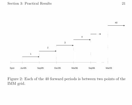
We have applied formula (28) to the Eurodollars market. There arecurrently 40 futures contracts being traded, which gives 40 forwardperiods, as figure 2 indicates.
Each forward period is chosen to be an interval between two pointsof the IMM grid, the first point corresponding to the maturity of thefutures contract. Note however that strictly speaking, a futures quoteimplies a futures rate corresponding to a period between the maturityof the contract, and this maturity +3 months. This period may not beexactly the one between two IMM points.14 This problem is referredto as the gap effect, which hopefully should not be significant.
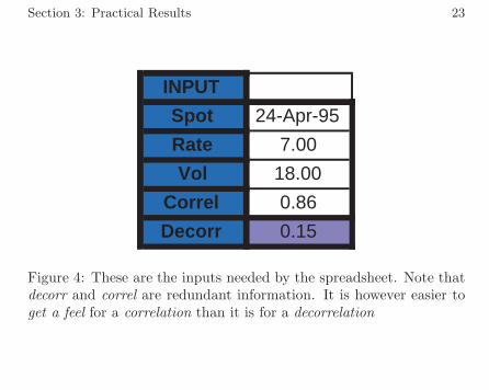
For each forward period, the convexity adjustment can be calcu-lated using formula (28). A possible set of inputs to this formula isshown in figure 4. As expected, Rate, Vol and Decorr refer to R∞, σand the decorrelation δ respectively. However, the latter is not a very
14 In other words, we want to know about forwards between IMM points, butwe only know about futures between IMM and IMM+3m.
Section 3: Practical Results 21
Jun95 Sep95 Dec95 Mar96 Sep96 Mar05Spot
1
2
3
4
40
Figure 2: Each of the 40 forward periods is between two points of theIMM grid.
Section 3: Practical Results 22
Futures rate vs maturityon 20 Apr 1995
0
1
2
3
4
5
6
7
8
9
Jun-
95
Dec
-95
Jun-
96
Dec
-96
Jun-
97
Dec
-97
Jun-
98
Dec
-98
Jun-
99
Dec
-99
Jun-
00
Dec
-00
Jun-
01
Dec
-01
Jun-
02
Dec
-02
Jun-
03
Dec
-03
Jun-
04
Dec
-04
Maturity of Futures contract
Fut
ures
rat
e
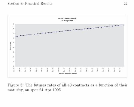
Figure 3: The futures rates of all 40 contracts as a function of theirmaturity, on spot 24 Apr 1995
Section 3: Practical Results 23
INPUT
Spot 24-Apr-95
Rate 7.00
Vol 18.00
Correl 0.86
Decorr 0.15
Figure 4: These are the inputs needed by the spreadsheet. Note thatdecorr and correl are redundant information. It is however easier toget a feel for a correlation than it is for a decorrelation
Section 3: Practical Results 24
t T T+∆T
T-t= ∆T T-t= ∆T
Futures Rate
Spot rate
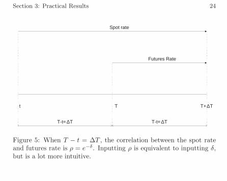
Figure 5: When T − t = ∆T , the correlation between the spot rateand futures rate is ρ = e−δ. Inputting ρ is equivalent to inputting δ,but is a lot more intuitive.
Section 3: Practical Results 25
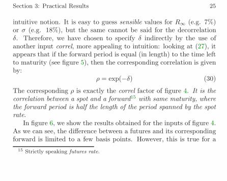
intuitive notion. It is easy to guess sensible values for R∞ (e.g. 7%)or σ (e.g. 18%), but the same cannot be said for the decorrelationδ. Therefore, we have chosen to specify δ indirectly by the use ofanother input correl, more appealing to intuition: looking at (27), itappears that if the forward period is equal (in length) to the time leftto maturity (see figure 5), then the corresponding correlation is givenby:
ρ = exp(−δ) (30)
The corresponding ρ is exactly the correl factor of figure 4. It is thecorrelation between a spot and a forward15 with same maturity, wherethe forward period is half the length of the period spanned by the spotrate.
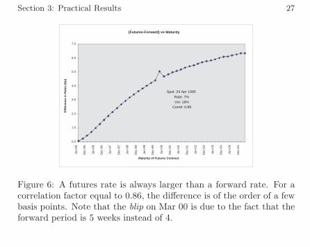
In figure 6, we show the results obtained for the inputs of figure 4.As we can see, the difference between a futures and its correspondingforward is limited to a few basis points. However, this is true for a
15 Strictly speaking futures rate.
Section 3: Practical Results 26
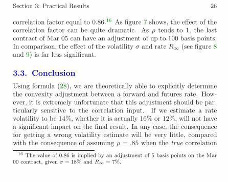
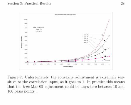
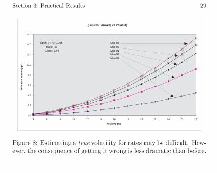
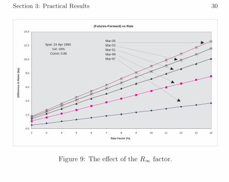
correlation factor equal to 0.86.16 As figure 7 shows, the effect of thecorrelation factor can be quite dramatic. As ρ tends to 1, the lastcontract of Mar 05 can have an adjustment of up to 100 basis points.In comparison, the effect of the volatility σ and rate R∞ (see figure 8and 9) is far less significant.
3.3. Conclusion
Using formula (28), we are theoretically able to explicitly determinethe convexity adjustment between a forward and futures rate. How-ever, it is extremely unfortunate that this adjustment should be par-ticularly sensitive to the correlation input. If we estimate a ratevolatility to be 14%, whether it is actually 16% or 12%, will not havea significant impact on the final result. In any case, the consequencefor getting a wrong volatility estimate will be very little, comparedwith the consequence of assuming ρ = .85 when the true correlation
16 The value of 0.86 is implied by an adjustment of 5 basis points on the Mar00 contract, given σ = 18% and R∞ = 7%.
Section 3: Practical Results 27
(Futures-Forward) vs Maturity
0.0
1.0
2.0
3.0
4.0
5.0
6.0
7.0
Jun-
95
Dec
-95
Jun-
96
Dec
-96
Jun-
97
Dec
-97
Jun-
98
Dec
-98
Jun-
99
Dec
-99
Jun-
00
Dec
-00
Jun-
01
Dec
-01
Jun-
02
Dec
-02
Jun-
03
Dec
-03
Jun-
04
Dec
-04
Maturity of Futures Contract
Diff
eren
ce in
Rat
es (
bp)
Spot: 24 Apr 1995Rate: 7%Vol: 18%
Correl: 0.86
Figure 6: A futures rate is always larger than a forward rate. For acorrelation factor equal to 0.86, the difference is of the order of a fewbasis points. Note that the blip on Mar 00 is due to the fact that theforward period is 5 weeks instead of 4.
Section 3: Practical Results 28
(Futures-Forward) vs Correlation
0.0
10.0
20.0
30.0
40.0
50.0
60.0
70.0
80.0
90.0
100.0
0.7 0.725 0.75 0.775 0.8 0.825 0.85 0.875 0.9 0.925 0.95 0.975 1
Correlation Factor
Diff
eren
ce in
Rat
es (
bp)
Spot: 24 Apr 1995Rate: 7%Vol: 18 %
Mar-05Mar-03Mar-01Mar-99Mar-97
Figure 7: Unfortunately, the convexity adjustment is extremely sen-sitive to the correlation input, as it goes to 1. In practice,this meansthat the true Mar 05 adjustment could be anywhere between 10 and100 basis points...
Section 3: Practical Results 29
(Futures-Forward) vs Volatility
0.0
2.0
4.0
6.0
8.0
10.0
12.0
14.0
16.0
4 6 8 10 12 14 16 18 20 22 24 26 28
Volatility (%)
Diff
eren
ce in
Rat
es (
bp)
Spot: 24 Apr 1995Rate: 7%
Correl: 0.86
Mar-05Mar-03Mar-01Mar-99Mar-97
Figure 8: Estimating a true volatility for rates may be difficult. How-ever, the consequence of getting it wrong is less dramatic than before.
Section 3: Practical Results 30
(Futures-Forward) vs Rate
0.0
2.0
4.0
6.0
8.0
10.0
12.0
14.0
2 3 4 5 6 7 8 9 10 11 12 13 14
Rate Factor (%)
Diff
eren
ce in
Rat
es (
bp)
Spot: 24 Apr 1995Vol: 18%
Correl: 0.86
Mar-05Mar-03Mar-01Mar-99Mar-97
Figure 9: The effect of the R∞ factor.
Section 3: Practical Results 31
is .95. It appears therefore that formula (28) is not sufficient in itself,to obtain both reliable and accurate estimate of the convexity adjust-ment. More information is needed on the correlation factor. One wayforward could be to regard the SWAP market as a benchmark provid-ing implied estimates. Another could be the use of historical data.17
As we can see, further research appears to be necessary.
References
[1] Doust, P. Relative pricing techniques in the swaps and optionsmarkets. To be published in the Journal of Financial Engineer-ing, Mar 95. 3, 15
[2] Doust,P. Convexity adjustment of futures prices into FRA rates.BZW, Debt Capital Markets. Internal document. 16, 17
17Although one tends to prefer implied data, making sure that historical esti-mates are not too far off is surely worth investigating.
Section 3: Practical Results 32
[3] Karatzas,I. and Shreve,S.E.(1991). Brownian motion andstochastic calculus. 2nd Ed. Springer-Verlag 35, 36, 36, 39, 42,45
List of Figures1 Correlation Assumption . . . . . . . . . . . . . . . . . 182 The IMM Grid . . . . . . . . . . . . . . . . . . . . . . 213 Yield Curve . . . . . . . . . . . . . . . . . . . . . . . . 224 Inputs to Model . . . . . . . . . . . . . . . . . . . . . 235 Estimating Decorrelation . . . . . . . . . . . . . . . . 246 Convexity Adjustment . . . . . . . . . . . . . . . . . . 277 Effect of Correlation . . . . . . . . . . . . . . . . . . . 288 Effect of Volatility . . . . . . . . . . . . . . . . . . . . 299 Effect of Rates Level . . . . . . . . . . . . . . . . . . . 30
Section A: appendix 33
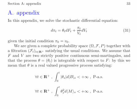
A. appendixIn this appendix, we solve the stochastic differential equation:
dπt = θtdFt +πtVtdVt (31)
given the initial condition π0 = v0.We are given a complete probability space (Ω,F , P ) together with
a filtration (Ft)t∈R+ satisfying the usual conditions. We assume thatF and V are two strictly positive continuous semi-martingales, andthat the process θ = (θt) is integrable with respect to F : by this wemean that θ is a real valued progressive process satisfying:
∀t ∈ R+ ,
∫ t
0
|θs|d|B|s < +∞ , P-a.s.
∀t ∈ R+ ,
∫ t
0
θ2sd〈M〉s < +∞ , P-a.s.
Section A: appendix 34
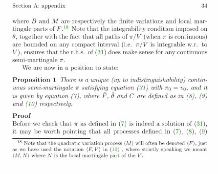
where B and M are respectively the finite variations and local mar-tingale parts of F .18 Note that the integrability condition imposed onθ, together with the fact that all paths of π/V (when π is continuous)are bounded on any compact interval (i.e. π/V is integrable w.r. toV ), ensures that the r.h.s. of (31) does make sense for any continuoussemi-martingale π.
We are now in a position to state:
Proposition 1 There is a unique (up to indistinguishability) contin-uous semi-martingale π satisfying equation (31) with π0 = v0, and itis given by equation (7), where F , θ and C are defined as in (8), (9)and (10) respectively.
ProofBefore we check that π as defined in (7) is indeed a solution of (31),it may be worth pointing that all processes defined in (7), (8), (9)
18 Note that the quadratic variation process 〈M〉 will often be denoted 〈F 〉, justas we have used the notation 〈F, V 〉 in (10) , where strictly speaking we meant〈M,N〉 where N is the local martingale part of the V .
Section A: appendix 35
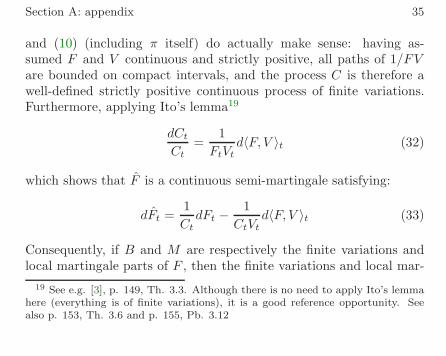
and (10) (including π itself) do actually make sense: having as-sumed F and V continuous and strictly positive, all paths of 1/FVare bounded on compact intervals, and the process C is therefore awell-defined strictly positive continuous process of finite variations.Furthermore, applying Ito’s lemma19
dCtCt
=1
FtVtd〈F, V 〉t (32)
which shows that F is a continuous semi-martingale satisfying:
dFt =1CtdFt −
1CtVt
d〈F, V 〉t (33)
Consequently, if B and M are respectively the finite variations andlocal martingale parts of F , then the finite variations and local mar-
19 See e.g. [3], p. 149, Th. 3.3. Although there is no need to apply Ito’s lemmahere (everything is of finite variations), it is a good reference opportunity. Seealso p. 153, Th. 3.6 and p. 155, Pb. 3.12
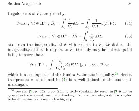
Section A: appendix 36
tingale parts of F , are given by:
P-a.s. , ∀t ∈ R+ , Bt =∫ t
0
1CsdBs −
∫ t
0
1CsVs
d〈F, V 〉s (34)
P-a.s. , ∀t ∈ R+ , Mt =∫ t
0
1CsdMs (35)
and from the integrability of θ with respect to F , we deduce theintegrability of θ with respect to F , the only may-be-delicate pointbeing to show that:
∀t ∈ R+ ,
∫ t
0
|θs|CsVs
d|〈F, V 〉|s < +∞ , P-a.s.
which is a consequence of the Kunita-Watanabe inequality.20 Hence,the process π as defined in (7) is a well-defined continuous semi-martingale.
20 See e.g. [3], p. 142, prop. 2.14. Strictly speaking the result in [3] is not asgeneral as the one used now, but extending it from square integrable martingales,to local martingales is not such a big step.
Section A: appendix 37
Checking that π is indeed solution of (31) is now straightforward:applying Ito’s lemma to (7), we obtain:
dπt = VtθtdFt +πtVtdVt + θtd〈F , V 〉t (36)
However, from (35), we have:
d〈F , V 〉t =1Ctd〈F, V 〉t (37)
and substituting (33) and (37) into (36), we obtain equation (31).We are now left with proving the uniqueness of π: suppose there
are two continuous semi-martingales with v0 as initial value and sat-isfying equation (31). Let X be their difference and define Y = X/V .Then X0 = 0 and X satisfies the equation:
dXt =Xt
VtdVt (38)
Section A: appendix 38
In particular, we have:
P-a.s. , ∀t ∈ R+ , 〈X,V 〉t =∫ t
0
Xs
Vsd〈V 〉s (39)
Furthermore, by Ito’s lemma:
d
(1Vt
)= − 1
V 2t
dVt +1V 3t
d〈V 〉t (40)
from which it is seen that:
dYt =1VtdXt −
Xt
V 2t
dVt +Xt
V 3t
d〈V 〉t −1V 2t
d〈X,V 〉t (41)
Substituting (38) and (39) into (41) shows that Y is indistinguishablefrom zero (Y0 = 0). This completes the proof of the uniqueness prop-erty. QED
Section B: appendix 39
B. appendixIn this appendix, we explicitly determine the process C as definedin (10) , and describe the assumptions made on F and V . We aregiven a complete probability space (Ω,F , P ) together with a two-dimensional standard Brownian motion (W,W ′) and the correspond-ing augmented Brownian filtration (Ft)t∈R+ . Given a borel mapρ : R+ → [−1, 1], we define the Brownian motion: 21
W ′′t4=∫ t
0
ρ(s)dWs +∫ t
0
√1− ρ2(s)dW ′s (42)
We assume that the processes F and V are given by F0, V0 > 0 andthe following:
dFt = µ(t)Ftdt+ σF (t)FtdWt (43)
Vt = exp(−(T + ∆T − t)Rt) (44)
21 W ′′ is a continuous (local) martingale with quadratic variation 〈W ′′〉t = t,hence it is a standard Brownian motion. See [3],p. 157,Th. 3.16
Section B: appendix 40
dRt = γ(R∞ −Rt)dt+ σR(t)R∞dW ′′t (45)
where γ,R∞ > 0 are constant, and µ, σF , σR are locally square inte-grable Borel maps on R+. We further assume that |σF | is boundedaway from zero, by a strictly positive constant. Note that F and Rare explicitly given by:22
Ft = F0 exp(∫ t
0
σF (s)dWs −12
∫ t
0
σ2F (s)ds+
∫ t
0
µ(s)ds)
(46)
Rt = R0e−γt +R∞(1− e−γt) +R∞e
−γt∫ t
0
eγsσR(s)dW ′′s (47)
Moreover, F and V are two strictly positive continuous semi-martin-gales, which shows that appendix A can legitimately be applied tothem.
22 The assumptions made on µ, σF and σR ensures that all integrals in (46)and (47) are meaningful. The reason for assuming |σF | bounded away from zero,and µ locally square integrable (as opposed to just locally integrable) will appearin appendix C.
Section B: appendix 41
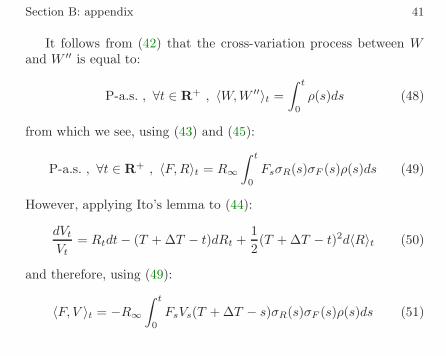
It follows from (42) that the cross-variation process between Wand W ′′ is equal to:
P-a.s. , ∀t ∈ R+ , 〈W,W ′′〉t =∫ t
0
ρ(s)ds (48)
from which we see, using (43) and (45):
P-a.s. , ∀t ∈ R+ , 〈F,R〉t = R∞
∫ t
0
FsσR(s)σF (s)ρ(s)ds (49)
However, applying Ito’s lemma to (44):
dVtVt
= Rtdt− (T + ∆T − t)dRt +12
(T + ∆T − t)2d〈R〉t (50)
and therefore, using (49):
〈F, V 〉t = −R∞∫ t
0
FsVs(T + ∆T − s)σR(s)σF (s)ρ(s)ds (51)
Section C: appendix 42
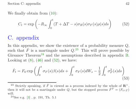
We finally obtain from (10):
Ct = exp(−R∞
∫ t
0
(T + ∆T − s)σR(s)σF (s)ρ(s)ds)
(52)
C. appendixIn this appendix, we show the existence of a probability measure Q,such that F is a martingale under Q.23 This will prove possible byGirsanov Theorem24 and the assumptions described in appendix B.Looking at (8), (46) and (52), we have:
Ft = F0 exp(∫ t
0
σF (s)β(s)ds +∫ t
0
σF (s)dWs −12
∫ t
0
σ2F (s)ds
)(53)
23 Strictly speaking, if F is viewed as a process indexed by the whole of R+,then it will not be a martingale under Q, but the stopped process FT = (Ft∧T )will.
24See e.g. [3] , p. 191, Th. 5.1
Section C: appendix 43
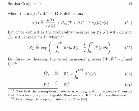
where the map β : R+ → R is defined as:
β(t)4=
µ(t)σF (t)
+R∞(T + ∆T − t)σR(t)ρ(t) (54)
Let Q be defined as the probability measure on (Ω,F) with densityZT with respect to P , where:25
ZT4= exp
(−∫ T
0
β(s)dWs −12
∫ T
0
β2(s)ds
)(55)
By Girsanov theorem, the two-dimensional process (W , W ′) definedby:26
Wt4= Wt +
∫ t∧T
0
β(s)ds (56)
W ′t4= W ′t (57)
25 Note that the assumptions made on µ, σF , σR and ρ in appendix B, ensurethat β is a locally square integrable Borel map on R+. So ZT is well-defined.
26Do not forget to stop your integral at T in (56).
Section C: appendix 44
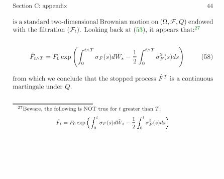
is a standard two-dimensional Brownian motion on (Ω,F , Q) endowedwith the filtration (Ft). Looking back at (53), it appears that:27
Ft∧T = F0 exp
(∫ t∧T
0
σF (s)dWs −12
∫ t∧T
0
σ2F (s)ds
)(58)
from which we conclude that the stopped process FT is a continuousmartingale under Q.
27Beware, the following is NOT true for t greater than T :
Ft = F0 exp
Z t
0σF (s)dWs −
1
2
Z t
0σ2F (s)ds
Section D: appendix 45
D. appendixIn this appendix, we show that the martingale representation theo-rem28 can actually be applied, to prove the existence of a constant x0
together with a process φ such that:
x0 +∫ T
0
φtdFt = α(FT −K) (59)
We shall also give a justification for formula (15).We first consider the complete probability space (Ω,F , Q), to-
gether with the augmented filtration (Gt)t∈R+ generated by the one-dimensional Brownian motion W .29 From equation (58), we have in
28 See e.g. [3], p.182, Th.4.15. However, we shall more specifically use one ofits corollaries: p.184, Pb. 4.17
29 Working on the right filtered probability space is of crucial importance here.Refer to appendix C for unexplained notations.
Section D: appendix 46
particular:
FT = F0 exp
(∫ T
0
σF (s)dWs −12
∫ T
0
σ2F (s)ds
)(60)
which shows that the random variable FT is Q-square integrable, andmeasurable with respect to GT . If we assume that the process C isdeterministic, then FT = FTCT (and therefore α(FT − K)) is itselfQ-square integrable and measurable with respect to GT .30
According to the martingale representation theorem, there exist aconstant x0 together with a (Gt)-progressive process y satisfying:
EQ
[∫ T
0
y2t dt
]< +∞ (61)
30 This is extremely important: if CT is random, we may still have the squareintegrability, but the measurability with respect to GT is lost for good. Note thatwe could relax slightly the assumption of C being deterministic, by just assumingCT non-random.
Section D: appendix 47
such that:
P-a.s. , x0 +∫ T
0
ytdWt = α(FT −K) (62)
Applying Ito’s lemma to (58), we have:
dFTt = σF (t)FTt dWT (63)
from which we obtain (59), provided φ is defined as φt = yt/σF (t).Finally, if we put v0 = x0V0 and θt = Vtφt/Ct
31, then φt = θtand therefore:
v0
V0+∫ T
0
θtdFt = α(FT −K)
and by (61), we see that t →∫ t∧T
0 ysdWs is a Q-square integrablemartingale, from which we conclude:
EQ
[∫ T
0
θtdFt
]= EQ
[∫ T
0
ytdWt
]= 0
31 Exercise: show that θ is integrable w.r. to F .


![RICCI CURVATURE OF FINITE MARKOV CHAINS VIA CONVEXITY … · Convexity along W-geodesics may thus be regarded as a discrete analogue of McCann’s displacement convexity [29], which](https://img.pdfslide.net/doc/110x75/5fdbdc573251aa62ea099ad8/ricci-curvature-of-finite-markov-chains-via-convexity-convexity-along-w-geodesics.jpg)


![Untitled Document [janroman.dhis.org]janroman.dhis.org/doc/AF.pdf · Title: Untitled Document Created Date: 10:52 7/2/2003](https://img.pdfslide.net/doc/110x75/5fa13a531f4af522244dd297/untitled-document-title-untitled-document-created-date-1052-722003.jpg)