Core Inflation and Trend Inflation

June 2015 (Revised November 2015)

James H. Stock

Department of Economics, Harvard University and the National Bureau of Economic Research

and

Mark W. Watson*

Department of Economics and the Woodrow Wilson School, Princeton University

and the National Bureau of Economic Research

*For helpful comments and discussion, we thank Marco del Negro, Giorgio Primiceri and seminar participants at the Universitat Pompeu Fabra EC2 conference, the National Bank of Belgium, the Society for Nonlinear Dynamics and Econometrics Oslo meetings, the Board of Governors of the Federal Reserve, and the Federal Reserve Bank of Richmond.

Abstract

An important input to monetary policymaking is estimating the current level of inflation. This

paper examines empirically whether the measurement of trend inflation can be improved by

using disaggregated data on sectoral inflation to construct indexes akin to core inflation but with

a time-varying distributed lags of weights, where the sectoral weight depends on the time-

varying volatility and persistence of the sectoral inflation series and on the comovement among

sectors. The model is estimated using U.S. data on 17 components of the personal consumption

expenditure inflation index. The modeling framework is a dynamic factor model with time-

varying coefficients and stochastic volatility as in del Negro and Otrok (2008); this is the

multivariate extension of the univariate unobserved components-stochastic volatility model of

trend inflation in Stock and Watson (2007). Our main empirical results are (i) the resulting

multivariate estimate of trend inflation is similar to the univariate estimate of trend inflation

computed using core PCE inflation (excluding food and energy) in the first half of the sample,

but introduces food in the second half of the sample; (ii) the model-based uncertainty about trend

headline inflation is substantially reduced by using the disaggregated series in a multivariate

model; (iii) the multivariate and univariate trends constructed using core measures of inflation

forecast average inflation over the 1-3 year horizon more accurately than a variety of other

benchmark inflation measures, although there is considerable sampling uncertainty in these

forecast comparisons.

JEL codes: C33, E31 Key words: inflation forecasts, non-Gaussian state space, time-varying parameters, dissagregated prices

 

  1

1. Introduction

A classic yet still-important problem of measuring the rate of price inflation is filtering

out the noise in inflation data to provide an estimate of the “trend” value of inflation. Following

Bryan and Cecchetti (1994), we think of trend inflation as the long-term estimate of the inflation

rate based on data on prices through the present. Having a good estimate of trend inflation is an

important input to monetary policy and to a myriad of private decisions. For example, as this is

written, a pressing question in the United States and the Eurozone is how far trend inflation is

below the 2% target. Because there are multiple sources of noise in inflation data and because

the nature of the noise can change over time, the task of estimating trend inflation is both

difficult and of ongoing relevance.

Producing an accurate estimate of trend inflation requires distinguishing persistent

variations in inflation from those that are unlikely to persist into the future. Broadly speaking,

there are two distinct approaches to this signal extraction problem.

The first approach is to use cross-sectional data on inflation (sectoral-level inflation data),

with a scheme that downweights sectors with large non-persistent variation. The most important

example of this approach is the standard measure of core inflation, which excludes food and

energy prices (Gordon (1975), Eckstein (1981); see Wynne (2008) for a discussion of the history

of core inflation). Other methods that exploit cross-sectional smoothing include trimmed means

or medians of sectoral inflation rates, see Bryan and Cecchetti (1994); these methods impose

zero/one weighting on each component, with weights that vary over time.1 For recent references

on core inflation see Crone, Khettry, Mester, and Novak (2013).

The second common approach to the signal extraction problem uses time-series

smoothing methods. Simple yet effective smoothers include the exponential smoother implied by

the IMA(1,1) model of Nelson and Schwert (1977) and the four-quarter average of quarterly

inflation (Atkeson and Ohanian (2001)). Stock and Watson (2007) and Cogley and Sargent

                                                            1 The Cleveland Fed publishes a median and trimmed mean CPI (https://www.clevelandfed.org/en/Our%20Research/Indicators%20and%20Data/Current%20Median%20CPI.aspx) and the Dallas Fed publishes a monthly trimmed mean PCE inflation index (http://www.dallasfed.org/research/pce/).

 

  2

(2015) provide methods that allow for time-variation in the smoother depending on changes in

the signal-to-noise ratio of the persistent and non-persistent components.

We follow this literature on core and trend inflation and consider estimates derived from

the price indexes and corresponding expenditure share weights used in the construction of the

headline inflation series of interest. A vast literature considers the problem of using other series,

such as measures of economic activity, interest rates, and terms of trade to forecast inflation. At

an abstract level, the distinction between using only price data, and price data combined with

other data, can be thought of as measurement vs. forecasting; the focus here is measurement. At

a practical level, at least for the U.S., some forecasting models using non-price data can improve

upon forecasts based solely on prices, but those improvements are small and, in many cases,

ephemeral. This underscores the practical relevance of estimates of trend inflation based on

constituent sectoral price data.

This paper combines the cross-sectional and time-series smoothing approaches to

examine four questions about the measurement of trend inflation and its relation to core inflation.

First, can more precise measures of trend inflation be obtained using disaggregated sectoral

inflation measures, relative to time series smoothing of aggregate ("headline") inflation? Second,

if there are improvements to be had by using sectoral inflation measures, do the implied sectoral

weights evolve over time or are they stable, and how do they compare to the corresponding

sectoral shares in consumption? Third, how do the implied time-varying weights and the

resulting multivariate estimate of trend inflation compare to conventional core inflation

measures? And fourth, do these trend inflation measures improve upon conventional core

inflation when it comes to forecasting inflation over the 1-3 year horizon?

We investigate these questions empirically using a univariate and multivariate

unobserved-components stochastic volatility outlier-adjusted (UCSVO) model that allows for

common persistent and transitory factors, time-varying factor loadings, and stochastic volatility

in the common and sectoral components. The time-varying factor loadings allow for changes in

the comovements across sectors, such as the reduction in energy price pass-through into other

prices. Introducing separate sectoral and common stochastic volatility in transitory and

permanent innovations allows for changes in the persistence of sectoral inflation and for sector-

specific changes in volatility. One source of the changing volatility in the component inflation

rates is changes in the methods and/or underlying data sources used to construct the historical

 

  3

series. A strength of the method used here is that the resulting estimates of historical trends

adjust for changes in measurement methods as well as for fundamental changes in the volatility

and persistence of the component series.

At a technical level, the model closest to that used here is del Negro and Otrok (2008),

which has time-varying factor loadings and stochastic volatility (their application is to

international business cycles, not inflation). Our model has some differences to fit our

application to U.S. sectoral inflation data, including distinct sectoral trends, a common trend, and

model-based detection of and adjustment for outliers.

The data we use are 17 sectors comprising the personal consumption expenditure (PCE)

price index for the United States, 1959Q1-2015Q2. Our main findings are: (i) the multivariate

trend estimates are more precise than the univariate estimates: posterior intervals for trend

inflation using the multivariate model are roughly one-third narrower than intervals based on

headline inflation alone; (ii) although the implied weights in the multivariate trend on most

sectoral components are close to their share weights, the implied weight on some series varies

substantially; (iii) broadly speaking, the multivariate trend estimate is a temporally smoothed

version of core (excluding food & energy) through the 1970s, but starting in the 1980s places

more weight on food (both off-premises and food services & accommodation) and less weight on

financial services, so that the composition of multivariate trend in the 2000s is roughly similar to

inflation for PCE excluding energy; and (iv) viewed as forecasts, the multivariate and univariate

trend estimates constructed using core inflation improve upon forecasts that use headline

inflation alone and several other benchmark forecasts, but the forecasting gains are imprecisely

estimated.

In addition to the literatures discussed above on core and trend inflation, this work is

related to three other large literatures. First, our modeling framework extends work estimating

common factors of multiple inflation series, including Bryan and Cecchetti (1993), Cristadoro,

Forni, Reichlin, and Veronese (2005), Amstad and Potter (2007), Kiley (2008), Altissimo,

Mojon, and Zaffaroni (2009), Boivin, Giannoni, and Mihov (2009), Reis and Watson (2010), and

Sbrana, Silvestrini, and Venditti (2015). Mumtaz and Surico (2012) introduce stochastic

volatility and time-varying factor dynamics into a model of 13 international inflation rates.

Second, the issues of including or excluding energy inflation is related to the literature on

changes in the pass-through of energy prices to headline or core inflation (something allowed for

 

  4

in our model); see Hooker (2002), De Gregorio, Landerretche, and Neilson (2007), van den

Noord and André (2007), Chen (2009), Blanchard and Galı (2010), Clark and Terry (2010), and

Baumeister and Peersman (2013). Also related is work that uses variables other than prices to

measure trend inflation, e.g. Mertens (2015), Garnier, Mertens, and Nelson (2015), and Mertens

and Nason (2015).

The next section presents the univariate and multivariate UCSVO models and discusses

their estimation. Section 3 provides the resulting univariate trend estimates for headline, core,

and PCE excluding energy. Section 4 presents multivariate results, first for the 17-sector model

then for a model with only three components: core, food, and energy. Section 5 compares the

forecasting performance of the various trend estimates over the 1-3 year horizon, and Section 6

concludes.

2. The Unobserved Components Model with Stochastic Volatility, Common Factors, and

Outlier Adjustment

The univariate UCSVO model. The univariate unobserved components/stochastic

volatility outlier-adjustment (UCSVO) model used in this paper expresses the rate of inflation as

the sum of a permanent and transitory component, where the innovations to both components

have variances that evolve over time according to independent stochastic volatility processes,

and where the innovation to the temporary component can have heavy tails (outliers):

πt = τt + εt (1)

τt = τt-1 + ,t × ,t (2)

t = ,t × st ,t. (3)

ln( 2,t ) = ,t (4)

ln( 2,t ) = ,t (5)

where (, , , ) are iidN(0, I4), and where st is an i.i.d. random variable that generates

outliers in t.

 

  5

This model expresses the rate of inflation πt as the sum of a permanent component τt

(trend) and a transitory component εt (1), in which τt follows a martingale (2) and the transitory

component is serially uncorrelated(3), and in which both innovations follow a logarithmic

random walk stochastic volatility processes (4) and (5). Conditional on the stochastic volatility

process, the transitory innovation εt is modeled in (3) as a mixture of normals via the i.i.d.

variable st, where st = 1 with probability (1 p), and st ~ U[2,10] with probability p. This

mixture model allows for outliers in inflation that is, large one-time shifts in the price level

which occur each period with probability p.

The UCSVO model (1) - (5) has only three parameters: γε and γτ govern the scale of the

innovation in the stochastic volatility process, and p governs the frequency of outliers. At a given

point in time, the autocovariance structure of πt is that of a IMA(1,1) process, however the outlier

distribution of the transitory innovation means that the estimate of t is not always well

approximated by the linear exponential smoother associated with a local IMA(1,1) filter.

This difference between (1) - (5) and the Stock-Watson (2007) UCSV model is that the

USCVO model includes an explicit model-based treatment of outliers. As will be seen below,

large infrequent spikes in inflation are observed in the data, especially in the sectoral

components.2 Stock and Watson (2007) made preliminary judgmental adjustments for outliers

prior to model estimation, however that approach is not feasible for real-time trend estimation

because it requires knowing whether a large change will mean-revert. Ignoring outliers is not

appealing because doing so runs the risk of mistaking a single large outlier for a more systematic

increase in the volatility of the transitory component. Because we are interested in real-time

trend estimation, (3) therefore extends the Stock-Watson (2007) model to make outlier

adjustments part of the model by modeling the transitory innovation as a mixture-of-normals.

The multivariate UCSVO model. This multivariate UCSVO (MUCSVO) model extends

the UCSVO model to include a common latent factor in both the trend and idiosyncratic

components of inflation, where the factor loadings are also time-varying. Let the subscripts c

denote the common latent factor and i denote the sector. The multivariate model is the del Negro

                                                            2 An example of such a sectoral outlier is the April 2009 increase in the Federal cigarette tax, which resulted in a 22% increase in cigarette prices that month. This tax increase drove a one-time jump in the rate of PCE inflation for other nondurable goods (the category that contains tobacco) in 2009Q2 of 10.4% at an annual rate, well above the 2.7% average rate of inflation for that category in 2008 and 2009 excluding that quarter.

 

  6

and Otrok (2008) dynamic factor model with time-varying factor loadings and stochastic

volatility, extended to have permanent and transitory components and to handle outliers in the

transitory disturbance.

The multivariate UCSV model is,

i,t = i,,t c,t + i,,t c,t + i,t + i,t, (6)

c,t = c,t-1 + ,c,t × ,c,t (7)

c,t = ,c,t × sc,t × ,c,t (8)

i,t = i,t-1 + ,i,t × ,i,t (9)

i,t = ,i,t × si,t × ,i,t (10)

i,,t = i,, t-1 + i, i,,t and i,,t = i,,t-1 + i, i,,t (11)

ln( 2, ,c t ) = ,c,c,t, ln( 2

, ,c t ) = ,c,c,t, ln( 2, ,i t ) = ,i,i,t, and

ln( 2, ,i t ) = ,i,i,t, (12)

where the disturbances (,c,t ,,c,t ,,i,t ,,i,t ,i,,t, i,,t,,c,t,,c,t,,i,t,,i,t) are i.i.d. standard

normal.

Equation (6) represents sector i inflation as the sum of a latent common factor for trend

inflation, τc,t, a latent common transient component, εc,t, and sector-specific trends and transient

components, i,t and i,t, and where the factor loadings evolve according to a random walk (11).

Equations (7) - (10) allow for stochastic volatility in the latent common and sector-specific

components, where the stochastic volatility evolves according to the logarithmic random walk

(12). Like the univariate model, the multivariate model allows for outliers in the common and

sectoral transitory components through the independent random variables sc,t and si,t in (8) and

(10), and where the outlier probabilities are pc and pi. The trend sectoral inflation is the sum of

the contribution of the common latent factor to that sector and the sectoral trend, that is, the

sectoral trend is i,,tc,t + i,t. The aggregate trend inflation is the sum of the sectoral trend,

weighted by the share weight wit of sector i in total inflation:

Aggregate trend = τt = , , , ,1

n

it i t c t i tiw

, (13)

 

  7

where n denotes the number of sectors.

The definition (13) of the aggregate trend τt nests a range of possibilities, from the

common trend providing all the trend movements in sectoral inflation (so that there are n-1

cointegrating vectors among the n sectors) to all sectoral inflation being independent with no

common trend. In this latter case, the common trend in aggregate inflation would just be the sum

of the idiosyncratic trends, weighted by the sectoral share weights.

Estimation. The model is estimated using Bayesian methods. The online appendix

contains a detailed description of the priors and the numerical methods used to approximate the

posteriors. We highlight a few details here.

In the univariate model, priors are needed for the stochastic volatility parameters and

, the outlier probability p, and the initial values 0, ln(,0), and ln(,0). We use independent

uniform priors for and that are calibrated so that the standard deviation of annual changes

in the values of ln(,t) and ln(,t) are distributed U[0,0.2]. The prior for p is Beta(,), where

and are calibrated to reflect information in a sample of length 10 years with an outlier

occurring once every 4 years. The priors for 0, ln(,0), and ln(,0) are independent diffuse

normal.

The priors for the multivariate model follow the priors used in the univariate model.

Thus, the priors for the various (, p) parameters and i,0, ln(i,,0), and ln(i,,0) are the ones

described in the last paragraph. The initial values of c,0 and i,0 are not separately identified, so

we set c,0 = 0. The factor structure of the multivariate model requires a normalization to

separately identify the scale of the factor loadings (, ) and factors (c, c), and this leads us to

set ln(,c,0) = ln(,c,0) = 0. We use an informative prior about the initial values of the factor

loadings: letting be the vector of factor loadings on c,t, the prior is ~ N(0, 21 ’ +

22 In)

where n is the number of sectors and is an n × 1 vector of 1’s. The parameter 1 governs the

prior uncertainty about the average value of factor loadings, and the parameter 2 governs the

variability of each factor loading from the average value. We set 1 = 10 (so the prior is

relatively uninformative about the average value of the factor loadings) and 2 = 0.4 (so there is

shrinkage toward the average values). The same prior is used for . The final set of parameters,

(i,, i,), govern the time variation in the factor loadings. Following Del Negro and Otrok

 

  8

(2008), we adopt an inverse Gamma prior for λ, with scale and shape parameters chosen so that

the prior corresponds to TPrior prior observations with 2Priors = 0.252/TPrior, where TPrior = T/10 and T

is the sample size.

Estimation of the posterior proceeds using Markov Chain Monte Carlo (MCMC)

methods. The stochastic volatility is handled following Kim, Shephard, and Chib (1998),

modified to use the Omori, Chib, Shephard, and Nakajima (2007) 10-component Gaussian

mixture approximation for the log-chi squared error. The MCMC iterations in Stock and Watson

(2007) have been corrected for an error pointed out by Del Negro and Primiceri (2014) that

applies generally to models with stochastic volatility. Details are presented in the online

appendix.

3. Data and Univariate Results

The data. The full data set consists of observations on 17 components of inflation used to

construct the PCE price index. The lowest-level components in NIPA Table 2.3.4 consist of 16

components (4 durable goods sectors, 4 nondurable good sectors, and 8 service sectors). Core

PCE excludes two of these 16 components (food for off-premises consumption and gasoline &

energy goods), and additionally excludes gas & electric utilities. Because gas & electric utilities

does not appear separately in Table 2.3.4, but rather is contained in housing & utilities, core PCE

cannot be constructed directly from these 16 components. So that our 17-sector treatment nests

core, we use data from NIPA tables 2.4.4 and 2.4.5 to further disaggregate housing & utilities

into gas & electric utilities and housing excluding gas & electric utilities, for a total of 17

sectoral components. Expenditure share weights for these components can be computed using

the nominal PCE values in NIPA tables 2.3.5 and 2.4.5. The raw data in the sample are monthly

observations from 1959M1-2015M6. Most of our analysis uses quarterly data constructed by

averaging the monthly inflation rates over the three months in the quarter. Throughout, inflation

is measured in percentage points at an annual rate. The 17 components and their expenditure

share weights for selected periods are given in Table 1.

In addition, we consider three aggregate indexes: the headline (all-components) PCE

price index (PCE-all), the Bureau of Economic Analysis’s PCE price index excluding energy

(PCExE), and the BEA core PCE price index excluding food and energy (PCExFE).

 

  9

The data are all final estimates of these series. Some of the component series have

undergone significant methodological changes over the years and have been subject to major

historical revisions. For example, in 2013 the price index for financial services was revised,

including changing the method for measuring implicitly priced services produced by commercial

banks (Hood (2013)). Prior to the revision, the category “financial services furnished without

payment” (e.g., checks processed without fees) used imputed prices based on market interest

rates, so those prices fluctuated substantially during periods of interest rate volatility. The 2013

revision changed the method for computing the reference interest rate for unpriced financial

services, reducing the volatility of this component. Because this revision was implemented

retroactively only to 1985, different methods are used to compute this component of the financial

services price index pre-1985 and post-1985.

As another example, in the 2009 revision, the category of food and tobacco (which until

then had been excluded from core) was distributed across three categories: food & beverages

purchased for off-premise consumption, other non-durable goods (which since 2009 includes

tobacco), and food services & accommodations; only the first of these is now excluded from core

PCE. Because the fully revised series reflect this change, it does not cause a break in the data

used in this paper, however it does mean that previous research on core PCE examined a

somewhat different concept than the current definition of core. Changing definitions and

measurement methods combined with partial historical adjustment are commonplace, and we

return to the implications of these methodological changes below.

Univariate results for PCE-all, PCExE, and PCExFE. Figure 1 plots headline (PCE-all)

and the two core inflation series (PCExE and PCExFE). Figure 2 plots the full-sample posterior

means for t , ,t, ,t, and st from the univariate model for each of these inflation measures.

The parameter values plotted in Figure 2 capture different features of the inflation series plotted

in Figure 1. Panel (a) of Figure 2 plots the posterior means for t. The broadly similar trend

estimates reflect the common low-frequency variability in the inflation series (see Figure 1),

however there are important differences between the univariate trend estimates, most notably

persistently higher trend inflation for PCE-all than for core inflation in the 2000s, and large but

less persistent deviations of the headline and core trends during the late 1970s and mid-1980s.

Over the entire sample period the mean absolute difference between the estimated trends in PCE-

all and PCExFE is 40 basis points, and is 20 basis points for the difference between PCExFE and

 

  10

PCExFE trends. In part, these differences reflect sampling errors associated with estimates, and

we present error bands below.

Panel (b) of Figure 2 shows estimates of ,t. These too are similar for the three inflation

series and reflect the larger trend variation in the first half of the sample (when trend inflation

increased during the 1970s and fell during the 1980s) than in the second half (when trend

inflation was relatively “anchored”).

Panel (c) of Figure 2 shows estimates of ,t. These show important variation both over

time and between inflation measure. Examination of PCE-all inflation in Figure 1 shows

relatively little high frequency volatility during the 1990s followed by a marked increase in

volatility in the early 2000s; this is reflected in the estimates for ,t in Figure 2. A more subtle

feature in Figure 1 is the difference between high frequency variability in the two core inflation

measures: their high frequency volatility are similar in the second half the sample, but PCExFE

exhibits much less high frequency than PCExE in the first half of the sample. This too is

reflected in the estimates of ,t for the two inflation series.

Finally, panel (d) of Figure 2 shows estimates of the outlier scale factors st. These factors

capture the outliers evident in all the inflation series plotted in Figure 1. (Note that st measures

outliers in standard deviation units, so that absolute size of outliers is larger for headline inflation

than the core measures of inflation.)

4. Multivariate Results

17-sector model. The multivariate model estimates many variables: the common

volatilities and trends (, c, t, ,c,t, c,t), their sector-specific counterparts (, i, t, ,i,t, i,t), the

sector-specific factor loadings (,i,t, ,i,t), the common and sector-specific outlier factors (sc,t,

si,t), and the aggregate inflation trend given in (13). The online appendix presents the model's

estimates for all of these variables, and we highlight a few of them here.

Figure 3 plots the MUCSVO model's full-sample estimates for the aggregate inflation

trend, and for comparison also plots the PCE-all UCSVO estimate. Broadly speaking, the

multivariate trend looks more like a time-averaged version of the two core measures (see Figure

2) than the univariate trend in PCE-all. The divergence between the univariate PCE-all trend and

the multivariate trend is largest in the 1970s, the mid 1980s, and the late 2000s. (Error bands for

 

  11

the estimates are discussed below.) Figure 3 also plots estimates of the volatility for the common

factors and common outliers. The time series of volatility for the common trend factor, ,c,t,

looks much like the trend volatility estimates from the UCSVO models, and ,c,t evolves much

like the corresponding estimates in the UCSVO models for core inflation.

Figure 4 shows estimates for the sector-specific variables for one sector, financial

services and insurance. (The online appendix contains the analogous figures for the other 16

sectors). As discussed in Section 3, the price index for the financial services and insurance sector

is measured differently before 1985 than after, and this measurement break is evident in the

sectoral inflation data plotted in Figure 4. The volatility of interest rates in the late 1970s and

early 1980s lead to large volatility in this sector's measured inflation resulting in a large increase

,i,t, the volatility of the sector-specific transitory term, it. Despite the break in measurement,

there is little evidence for a break in the factor loadings, although these are estimated

imprecisely. There are several sector-specific outliers, both before and after the break in

measurement.

The similarities between the estimated trend in the MUCSVO model and the univariate

UCSVO estimates using the core inflation measures raise the question of whether the

multivariate trend is in effect a temporally smoothed version of core inflation and, more

generally, what are the time-varying weights implicitly used in the multivariate trend. At any

given point in time, the one-sided estimates from the multivariate trend is a nonlinear function of

current and past values of the 17 sectoral inflation rates. Because of the time-varying parameters

in the MUCSVO model, these weights evolve over time, and they involve lags because of the

time series smoothing implied by the model. The function of current and past values is also

nonlinear because of the outlier variable. For these reasons, an exact representation in terms of a

time-varying linear weighted average is not feasible. Nevertheless, useful insights into the cross-

sectional smoothing can be obtained by looking at approximate time-varying weights.

Specifically, at a given date, a linear approximation to the one-sided trend estimates can be

computed using a Kalman filter based on (6) – (10), holding fixed the values of the time-varying

factor loadings and volatilities (c,t, i,t, ln( 2, ,c t ), ln( 2

, ,c t ). ln( 2, ,i t ), and ln( 2

, ,i t )) at

their full-sample posterior mean values at that date and ignoring outliers by setting sc,t = si,t = 1.

(The online appendix describes these calculations in more detail.)

 

  12

Figure 5 plots the approximate linear weights on the 17 components implicit in the one-

sided multivariate estimate of the trend, specifically, the sum of the weights on the current and

first three lagged values of the component inflation series. Comparing the approximate

MUCSVO weight to the expenditure share shows whether, at a given date, the sector is getting

more or less weight in the MUCSVO trend than it does in PCE-all.

As can be seen in Figure 5, roughly half of the 17 components receive weight similar to

their expenditure shares. The fact that so many of these weights track expenditure shares is by

itself interesting, since the expenditure shares are not used in the MUCSVO model (expenditure

shares are used in (13) to construct the overall trend based on the 17 filtered individual trends

and the filtered common trend, but not in the calculation of the estimates of the individual and

common trends). Components with weights that track expenditure shares include recreational

goods & vehicles, other durable goods, other nondurable goods, housing excluding energy

services, health care, transportation services, other services, and NPISHs.

Other series have large swings in their weights. The weight on food & beverages for off-

premises consumption (“food at home”) increases substantially and, since the mid-1990s,

essentially equals its expenditure share, and the weight on food services & accommodations rises

from its share in the mid-1970s to nearly double its share in the 1980s and 1990s. Relative to

their expenditure shares, the weights fell on financial services & insurance (since the late 1970s),

on clothing and footwear (since the early 1980s), on furnishings & durable household equipment

(since the mid-1980s), and on gas & electric utilities (since the mid-1990s). Except during the

1960s, gasoline & energy goods receives essentially zero weight.

Figure 6 shows these sectoral weights aggregated to core, food, and energy, where food is

food for off-premises consumption, energy is gasoline & other energy goods and gas & electric

utilities, and core consists of the remaining 14 sectors. As can be seen from these weights, the

multivariate trend estimate evolved to increase the weight on food, and to decrease the already-

low weight on energy, around 1990.

To better understand the reasons for these time-varying weights, we now take a closer

look at four of the sectoral inflation rates. Figure 7 plots time series for these inflation rates along

with posterior median and (point-wise) 67% posterior intervals for the standard deviation of their

idiosyncratic noise components, ,i,t. The first inflation series is for food services &

accommodations. Inflation in this sector tracks PCE-all inflation for the full sample, but has

 

  13

higher idiosyncratic volatility in the 1960s and 1970s. The reduction in the post-1970s

idiosyncratic volatility makes this series a better indicator of trend inflation and thus the series

receives more weight in the trend estimate beginning in the late 1970s.

The next inflation series shown in Figure 7 is for food & beverages for off-premises

consumption. This series is noisy early in the first half of the sample but less so later in the

sample. The decrease in volatility of its idiosyncratic transitory innovation makes it a better

indicator of trend inflation, so its weight in the estimate of trend inflation increases in the second

half of the sample even though its expenditure share is falling.

The third series is furnishing & durable household equipment, which smoothly tracks

PCE inflation early in the sample but diverges and exhibits increased volatility since around

1990. While this component receives considerable weight – more than twice its expenditure

share – in the MUCSVO trend in the pre-1980 period, its weight drops to its expenditure share

since 1990.

The final series is gasoline & other energy goods, which since the early 1970s has

exhibited volatility that is an order of magnitude large than the other sectoral inflation measures.

Variations in this series are a poor indicator of trend inflation and the series receives essentially

zero-weight in the estimated MUCSVO trend.

Three-sector model. The results for the 17-sector model raise the question of whether

similar results can be obtained using a simpler 3-sector model consisting of core (PCExFE),

energy (the two energy components excluded from core, combined with their share weights), and

food (off-premises). We therefore estimated this 3-component model using the multivariate

model of Section 2. Selected results for this model are presented below, and detailed results are

available in the online appendix

Accuracy of the trend estimates. One of the motivating questions of this work is whether

using sectoral information can improve the precision of the estimator of the trend in headline

inflation. Because trend inflation is never observed, the precision of the various estimators

cannot be computed directly from the data. In this section we present model-based accuracy

measures based on the width of posterior uncertainty intervals, which are complemented in the

next section with a pseudo-out-of-sample forecast experiment.

Panel (a) of Figure 8 plots point-wise 90% posterior intervals for the trend in PCE-all

computed from the UCSVO and 17-component MUCSVO models. The width of these intervals

 

  14

reflects two distinct sources of uncertainty: (i) signal extraction uncertainty conditional on values

of the model's parameters, and (ii) uncertainty about the model parameters. Because the

information set for the multivariate model is strictly larger than univariate model, signal

extraction uncertainty is smaller in the MUCSVO model. However, many more parameters are

estimated in the MUCSVO model, so parameter uncertainty may be larger, and therefore there is

no a priori ranking of the width of posterior intervals in the UCVSO and MUCSVO models.

Examination of panel (a) shows that the MUCSVO intervals are visibly narrower than the

UCSVO bands, suggesting a substantial reduction in uncertainty using the information in the

multivariate model, even at its cost of additional complexity. Panel (a) of Table 2 summarizes

these results by showing the average width of 67% and 90% posterior intervals for the UCSVO

and MUCSVO models over the first and second halves of the sample. The 67% and 90% full-

sample posterior intervals for the PCE-all trend (labeled PCE‐allt in the table) are roughly 35%

narrower than the corresponding intervals for the univariate model.

Figure 9 shows the corresponding intervals, but for posteriors computed recursively using

data from the beginning of the sample through time t. We compute these one-sided posteriors

beginning in t = 1990:Q1 and continuing through the end of the sample (2015Q2). Because these

one-sided intervals use less information that the full-sample posteriors they are necessarily

wider, but as the values in panel (b) indicate, the 17-component MUCSVO model again produces

intervals that are roughly 40% narrower than UCSVO model.

The MUCSVO model can also be used to estimate the trend in the core measures of

inflation, PCExE and PCExFE, by using equation (13), but with share weights (wit) appropriate

for these measures. Comparisons of the posterior intervals for these multivariate estimates and

their univariate counterparts are shown in panels (b) and (c) of Figures 8 and 9, and the average

widths of these intervals are shown in Table 2. The relative improvements of the accuracy of the

multivariate models are much smaller for estimates of the trend in these core measures of

inflation. For example, the one-sided multivariate intervals are 10-15 percent narrower than their

univariate counterparts for core inflation, compared to 40 percent narrower for headline inflation.

And the relative gains for the full-sample estimates are even less.

The final panel in Figures 8 and 9 compare the 3-component and 17-component

MUCSVO intervals for the trend in headline inflation. The average widths in Table 2 suggest

that some, but not all of the accuracy gains for estimating PCE-all are achieved by the 3-

 

  15

component model. Interesting, for estimating the trends in core inflation, the 3-component

MUCSVO model produces intervals that are wider than the univariate models indicating that the

increased parameter uncertainty outweighs the signal extraction information.

5. Forecasting performance

The definition of trend inflation as the forecast of inflation over the long run suggests

using forecasting performance to evaluate candidate estimates of trend inflation. Following much

of the literature on inflation forecasting using core inflation, we focus on forecasts at the 1-3 year

horizon.

Specifically, we use the one-sided posterior mean estimates of t, denoted by t|t and

described in the last section, from the various models to forecast the average value of inflation

over the next 4, 8, and 12 quarters, that is to forecast

PCE‐all 1 PCE‐all1: 1

h

t t h t iih for h = 4, 8, and 12

and where PCE‐allt is the date t value of PCE-all inflation. Forecasts are constructed using PCE‐all/t t ,

constructed from the univariate UCSVO and 3- and 17-component MUCSVO models and from

PCExE/t t and t/tPCExFE computed from univariate UCSVO models. The variable being forecast is

headline inflation, PCE‐all1:t t h , in all of the experiments even when being forecast by the core trend

estimates. We also consider six benchmark forecasts: random walk models using (separately)

lagged PCE-all, lagged PCExE, and lagged PCExFE, and the Atkeson-Ohanian (2001) four-

quarter random walk model computed using (separately) PCE-all, PCExE, and PCExFE.

Forecasts are constructed from t = 1990:Q1 through the end of the sample

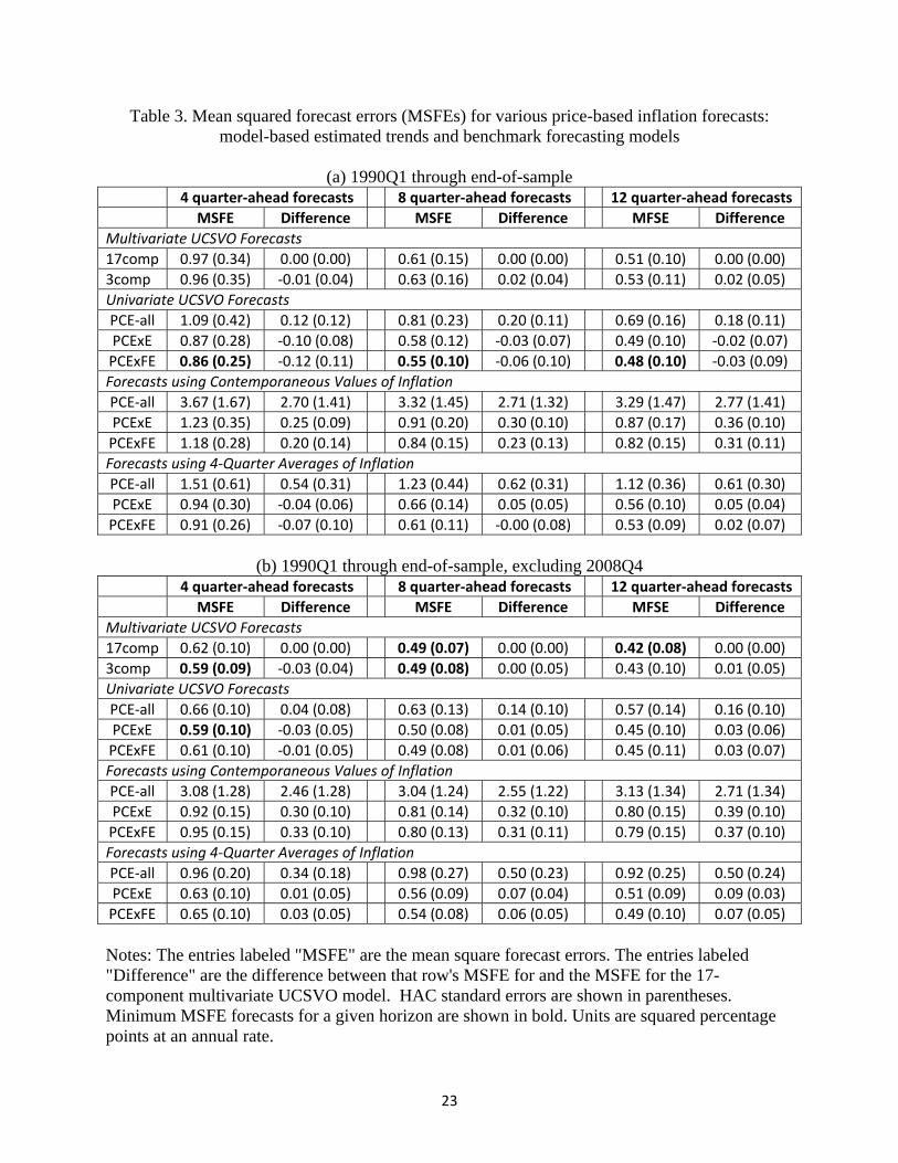
Table 3 summarizes the results. Panel (a) shows results for the entire 1990Q1 – end of

sample period. For each forecast the table reports the sample mean square forecast error (MSFE)

together with its estimated standard error, and the difference between the forecast's MSFE and

the MSFE of the 17-component MUCSVO model, together with its standard error. The values of

these MSFEs are greatly affected by the large outlier in PCE‐all2008 4Q evident in Figure 1. Panel (b)

shows results from the same forecasting exercise, but with this single observation omitted from

the sample values of PCE‐all1:t t h . We concentrate our discussion on the panel (b) results.

 

  16

Four results stand out from this forecasting experiment. First, forecasts that use moving

averages of past inflation are more accurate than forecasts that do not. All of the moving-average

forecasts (from the simple 4-quarter moving averages to the more sophisticated moving averages

in the UCSVO and MUCSVO models) produce markedly more accurate forecasts than the

corresponding forecasts using only contemporaneous values of inflation. Second, forecast

accuracy is improved by down-weighting some sectors, most notably energy. Forecasts that put

little or no weight on energy, whether by using the core inflation measures or the MUCSVO

models, are more accurate that forecasts based on headline inflation, regardless of the moving

average filter used. Third, the UCSVO forecasts have smaller MSFE than the 4-quarter moving

average forecasts, suggesting that there are gains from using forecasts that adapt to the changing

persistence in the inflation process. And finally, there are only small (perhaps zero) marginal

improvements in accuracy for the MUCSVO forecasts relative to the core-inflation UCSVO

forecasts.

6. Discussion and Conclusions

Previous work has shown that the random-walk-plus-white-noise unobserved components

model with stochastic volatility provides a simple but flexible univariate framework for

describing the persistence and volatility of inflation, for estimating its trend, and for forecasting

future inflation. This paper has investigated a multivariate extension of that model that allows

sectoral inflation potentially to improve upon the univariate estimates of trend inflation, much

like traditional core inflation does for headline inflation.

The analysis leads to two major conclusions. First, there are substantial gains from using

sectoral inflation over using headline inflation. The multivariate estimates of the trend in

aggregate (headline) inflation are more accurate than the univariate estimates regardless of

whether accuracy is measured by model-based uncertainty or pseudo-out-of-sample forecasting

accuracy. But second, the analysis suggests that much of this improved accuracy can be

achieved from univariate estimates constructed from traditional core measures of inflation.

Model-based uncertainty measures suggest that univariate estimates of the trend in core inflation

are nearly as accurate as multivariate estimates of these same trends. Moreover, the pseudo-of-

 

  17

sample experiments suggest little difference in the accuracy of these estimates of core trend

inflation for forecasting future headline inflation.

The results also lead to two other conclusions. The first is that the reduced volatility of

food prices, relative to before the mid-1980s, led the multivariate model to include food in the

trend estimate post-1990, with a weight close to its expenditure share. This finding suggests

paying more attention to PCExE than to PCExFE. Second, the UCSVO models (univariate or

multivariate) have the advantage of producing measures of precision of trend estimates (posterior

coverage regions). Currently, the width of these 67% regions is approximately 0.6 percentage

point using the 17-variable or univariate core trend estimates. We see merit to reporting these

estimates of the precision of trend inflation along with estimates of that trend.

Finally, we highlight three areas where the analysis might be extended. First, there are a

myriad of ways the multivariate model might be changed by, for example, including additional

factors, restricting the factor loadings, or allowing for different dynamics. We experimented with

several of these before settling on the specification used here, but our experiments were far from

exhaustive. Second, we investigated 3- and 17- component models, but much finer sectoral

dissagregation is possible. Our initial look at more finely dissagregated data suggested

substantial challenges associated with instability in measurement, but clever modeling might

address those challenges. Finally, and most important, this analysis has used quarterly averages

of monthly inflation rates. Real-time analysis would benefit from directly modeling the monthly

data. Our experiments applying the UCSVO and MUCSVO models directly to the monthly data

yielded forecasts that were less accurate than the forecasts from the quarterly data. (Results are

reported in the online appendix.) This suggests that a successful monthly model will require

alternative specifications for the transitory and trend innovations.

 

  18

References

Altissimo, Filippo, Benoit Mojon, and Paolo Zaffaroni (2009). “Can Aggregation Explain the

Persistence of Inflation?” Journal of Monetary Economics 56(2), 231-241.

Amstad, Marlene, and Simon M. Potter (2007). “Real Time Underlying Inflation Gauges for

Monetary Policy Makers.” Unpublished manuscript, Federal Reserve Bank of New York

Atkeson, A. and L.E. Ohanian (2001), “Are Phillips Curves Useful for Forecasting Inflation?”

Federal Reserve Bank of Minneapolis Quarterly Review 25(1):2-11.

Baumeister, Christiane and Gert Peersman. 2013. “Time-Varying Effects of Oil Supply Shocks

on the U.S. Economy.” American Economic Journal: Macroeconomics, vol. 5, pp. 1-28.

Blanchard, Olivier J., and Jordi Galí. 2010. “The Macroeconomic Effects of Oil Price Shocks:

Why Are the 2000s So Different from the 1970s?” In International Dimensions of

Monetary Policy, edited by Jordi Galí and Mark J.Gertler. University of Chicago Press.

Boivin, Jean, Marc P. Giannoni, and Ilian Mihov (2009). “Sticky Prices and Monetary Policy:

Evidence from Disaggregated Data.” American Economic Review, 99(1): 350–84.

Bryan, Michael F. and Cecchetti, Stephen G. (1993), "The Consumer Price Index as a Measure

of Inflation," Federal Reserve Bank of Cleveland, Economic Review, December: 15-24.

Bryan, Michael F. and Cecchetti, Stephen G. (1994). “Measuring Core Inflation,” in N. Gregory

Mankiw, ed., Monetary Policy. Chicago: University of Chicago Press, pp. 195-215.

Chen, Shiu-Sheng (2009). “Oil Price Pass-Through into Inflation.” Energy Economics 31(1):

126-133.

Crone, T. M., Khettry, N. N. K., Mester, L. J. and Novak, J. A. (2013), "Core Measures of

Inflation as Predictors of Total Inflation." Journal of Money, Credit and Banking,

45: 505–519.

Clark, Todd E. (1999) “A Comparison of the CPI and the PCE Price Index.” Federal Reserve

Bank of Kansas City, Economic Review, 84 (Third Quarter), 15–29.

Clark, Todd E. (2001) “Comparing Measures of Core Inflation.” Federal Reserve Bank of

Kansas City, Economic Review, 86 (Second Quarter), 5–31.

Clark, Todd E. and Stephen J. Terry (2010). “Time Variation in the Inflation Passthrough of

Energy Prices,” Journal of Money, Credit and Banking 42(7), 1419-1433.

 

  19

Cogley, Timothy. (2002) “A Simple Adaptive Measure of Core Inflation.” Journal of Money,

Credit, and Banking, 34, 94–113.

Cogley, Timothy and Thomas J. Sargent (2015). “Measuring Price-Level Uncertainty and

Instability in the U.S., 1850-2012,” The Review of Economics and Statistics, forthcoming.

Cristadoro, Riccardo, Mario Forni, Lucrezia Reichlin, and Giovanni Veronese (2005), "A Core

Inflation Indicator for the Euro Area," Journal of Money, Credit, and Banking, Vol. 37,

No. 3, pp. 539-560.

Crone, Theodore M., N. Neil K. Khettry, Loretta J. Mester, and Jason A. Novak (2013). “Core

Measures of Inflation as Predictors of Total Inflation,” Journal of Money, Credit and

Banking 45, no. 2-3, 505-519.

De Gregorio, José, Oscar Landerretche, and Christopher Neilson (2007). “Another Pass-through

Bites the Dust? Oil Prices and Inflation.” Economia 7(2), 155-208.

Eckstein, Otto (1981). Core Inflation. New York: Prentice Hall, 1981.

Garnier, Christine, Elmar Mertens, and Edward Nelson (2015). “Trend Inflation in Advanced

Economies.” International Journal of Central Banking, forthcoming.

Gordon, Robert (1975). “Alternative Responses of Policy to External Supply Shocks.” Brookings

Papers on Economic Activity, volume 1, pp. 183 – 206.

Hood, Kyle K. (2013) “Measuring the Services of Commercial Banks in the National Income

and Products Accounts: Changes in Concepts and Methods in the 2013 Comprehensive

Revision.” Survey of Current Business, February 2013, 8-19.

Hooker, Mark A. (2002). “Are Oil Shocks Inflationary? Asymmetric and Nonlinear

Specifications versus Changes in Regime,” Journal of Money, Credit, and Banking 34(2),

540-561.

Kiley, Michael T. (2008), "Estimating the common trend rate of inflation for consumer prices

and consumer prices excluding food and energy," FEDS working paper 2008-38.

Kim, Sanjoon, Neil Shephard and Siddhartha Chib (1998). “Stochastic Volatility: Likelihood

Inference and Comparison with ARCH Models,” Review of Economic Studies, 65, 361-

393.

Mertens, Elmar (2015). “Measuring the level and uncertainty of trend inflation.” Review of

Economics and Statistics, forthcoming.

 

  20

Mertens, Elmar and James M. Nason (2015). “Inflation and Professional Forecast Dynamics: An

Evaluation of Stickiness, Persistence, and Volatility.” Manuscript. Board of Governors of

the Federal Reserve System, Washington, D.C.

Mumtaz, Haroon and Paolo Surico (2012). “Evolving International Inflation Dynamics: World

and Country-Specific Factors.” Journal of the European Economics Association 10(4),

716-734.

del Negro, Marco and Christopher Otrok (2008). “Dynamic factor models with time-varying

parameters: Measuring changes in international business cycles.” Staff Report, Federal

Reserve Bank of New York, no. 326.

del Negro, Marco and Giorgio E. Primiceri (2014). “Time Varying Structural Vector

Autoregressions and Monetary Policy: A Corrigendum.” Review of Economic Studies,

forthcoming.

Nelson, C.R. and G.W. Schwert (1977), “Short-Term Interest Rates as Predictors of Inflation:

On Testing the Hypothesis that the Real Rate of Interest Is Constant,” American

Economic Review 67:478-486.

Omori, Yasuhiro, Siddhartha Chib, Neil Shephard, and Jouchi Nakajima, (2007). “Stochastic

Volatility with Leverage: Fast and Efficient Likelihood Inference,” Journal of

Econometrics 140(2), 425-449.

Reis, Ricardo, and Mark W. Watson. (2010) “Relative Goods’ Prices, Pure Inflation, and the

Philips Correlation.” American Economic Journal: Macroeconomics, 2, 128-57.

Rich, Robert, and Charles Steindel. (2005) “A Review of Core Inflation and an Evaluation of Its

Measures.” Federal Reserve Bank of New York Staff Report 236.

Sbrana, Giacomo, Andrea Silvestrini, and Fabrizio Venditti (2015). “Short Term Inflation

Forecasting: The M.E.T.A. Approach.” Manuscript, Bank of Italy.

Stock, James H. and Mark W. Watson (2007), ”Why Has U.S. Inflation Become Harder to

Forecast?”, Journal of Money, Credit and Banking, 39(1), 3-33.

van den Noord, Paul and Christophe André (2007). “Why Has Core Inflation Remained So

Muted in the Face of the Oil Shock?” OECD Economics Department Working Paper 551.

Wynne, Mark A. (2008). “Core Inflation: A Review of Some Conceptual Issues,” Federal

Reserve Bank of St. Louis Review, May/June 2008, 90(3 Part 2), 205-28.

 

  21

Table 1. The 17 Components of the PCE Price IndsUsed in this Study and their Expenditure Shares

Sector  1960‐2015 

1960‐1979 

1980‐1999 

2000‐2015 

Durable goods         

Motor vehicles and parts 0.053 0.060 0.054  0.042

Furnishings and durable household equipment 0.036 0.044 0.033  0.028

Recreational goods and vehicles 0.029 0.026 0.029  0.032

Other durable goods 0.016 0.015 0.016  0.016

Nondurable goods         

Food and beverages purchased for off‐premises consumption*

0.117 0.160 0.104  0.077

Clothing and footwear 0.054 0.071 0.051  0.034

Gasoline and other energy goods* 0.037 0.044 0.035  0.032

Other nondurable goods 0.078 0.080 0.074  0.081

Services         

Housing & utilities         Housing excluding gas & electric utilities 0.153 0.146 0.155  0.161

Gas & electric utilities*  0.025  0.026  0.028  0.021 

Health care 0.114 0.071 0.127  0.155

Transportation services 0.032 0.030 0.034  0.032

Recreation services 0.029 0.021 0.031  0.038

Food services and accommodations 0.064 0.064 0.066  0.061

Financial services and insurance 0.063 0.047 0.068  0.076

Other services 0.081 0.081 0.077  0.087

Final consumption expenditures of nonprofit institutions serving households (NPISHs)

0.020 0.016 0.019  0.026

Notes: Each column shows the average expenditure share over the sample period indicated. *Excluded from core PCE.  

 

  22

Table 2: Average width of 90% posterior intervals for trend inflation.

(a) Full-sample Posterior Inflation Trend 

Univariate    Multivariate 

3 Components    17 Components 

1960‐1989  1990‐2015    1960‐1989  1990‐2015    1960‐1989  1990‐2015 

  67% Intervals 

PCE‐All  1.17  0.75    0.88  0.55    0.75  0.48 

PCExE  1.02  0.46  0.85  0.48  0.74  0.42 

PCExFE  0.78  0.42  0.81  0.49  0.68  0.41 

  90% Intervals 

PCE‐All  2.03  1.32    1.53  0.96    1.27  0.83 

PCExE  1.77  0.79  1.48  0.83  1.25  0.72 

PCExFE  1.37  0.73  1.41  0.85  1.15  0.71 

(b) One-Sided Posterior, 1990-2015

Inflation Trend 

Univariate    Multivariate 

3 Components    17 Components 

  67% Error Bands 

PCE‐All  1.06    0.75    0.64 

PCExE  0.66  0.67  0.57 

PCExFE  0.62  0.68  0.57 

  90% Error Bands 

PCE‐All  1.88    1.31    1.10 

PCExE  1.15  1.18  0.99 

PCExFE  1.09  1.20  0.99 

Notes: The table shows the average width of (equal-tailed, point-wise) posterior intervals for the inflation trends listed in the first column. Panel (a) uses the full-sample posterior. Panel (b) uses a sequence of one-sided posteriors using samples ending in period t, for t = 1990Q1 through 2015Q2.

 

  23

Table 3. Mean squared forecast errors (MSFEs) for various price-based inflation forecasts: model-based estimated trends and benchmark forecasting models

(a) 1990Q1 through end-of-sample

  4 quarter‐ahead forecasts    8 quarter‐ahead forecasts    12 quarter‐ahead forecasts 

  MSFE  Difference    MSFE  Difference    MFSE  Difference 

Multivariate UCSVO Forecasts 

17comp   0.97 (0.34)  0.00 (0.00)    0.61 (0.15)  0.00 (0.00)    0.51 (0.10)  0.00 (0.00)  

3comp  0.96 (0.35)  ‐0.01 (0.04)    0.63 (0.16)  0.02 (0.04)    0.53 (0.11)  0.02 (0.05)  

Univariate UCSVO Forecasts 

PCE‐all  1.09 (0.42)  0.12 (0.12)    0.81 (0.23)  0.20 (0.11)    0.69 (0.16)  0.18 (0.11)  

PCExE  0.87 (0.28)  ‐0.10 (0.08)    0.58 (0.12)  ‐0.03 (0.07)    0.49 (0.10)  ‐0.02 (0.07)  

PCExFE  0.86 (0.25)  ‐0.12 (0.11)    0.55 (0.10)  ‐0.06 (0.10)    0.48 (0.10)  ‐0.03 (0.09)  

Forecasts using Contemporaneous Values of Inflation  

PCE‐all  3.67 (1.67)  2.70 (1.41)    3.32 (1.45)  2.71 (1.32)    3.29 (1.47)  2.77 (1.41)  

PCExE  1.23 (0.35)  0.25 (0.09)    0.91 (0.20)  0.30 (0.10)    0.87 (0.17)  0.36 (0.10)  

PCExFE  1.18 (0.28)  0.20 (0.14)    0.84 (0.15)  0.23 (0.13)    0.82 (0.15)  0.31 (0.11)  

Forecasts using 4‐Quarter Averages of Inflation 

PCE‐all  1.51 (0.61)  0.54 (0.31)    1.23 (0.44)  0.62 (0.31)    1.12 (0.36)  0.61 (0.30)  

PCExE  0.94 (0.30)  ‐0.04 (0.06)    0.66 (0.14)  0.05 (0.05)    0.56 (0.10)  0.05 (0.04)  

PCExFE  0.91 (0.26)  ‐0.07 (0.10)    0.61 (0.11)  ‐0.00 (0.08)    0.53 (0.09)  0.02 (0.07)  

(b) 1990Q1 through end-of-sample, excluding 2008Q4

  4 quarter‐ahead forecasts    8 quarter‐ahead forecasts    12 quarter‐ahead forecasts 

  MSFE  Difference    MSFE  Difference    MFSE  Difference 

Multivariate UCSVO Forecasts 

17comp   0.62 (0.10)  0.00 (0.00)    0.49 (0.07)  0.00 (0.00)    0.42 (0.08)  0.00 (0.00)  

3comp  0.59 (0.09)  ‐0.03 (0.04)    0.49 (0.08)  0.00 (0.05)    0.43 (0.10)  0.01 (0.05)  

Univariate UCSVO Forecasts 

PCE‐all  0.66 (0.10)  0.04 (0.08)    0.63 (0.13)  0.14 (0.10)    0.57 (0.14)  0.16 (0.10)  

PCExE  0.59 (0.10)  ‐0.03 (0.05)    0.50 (0.08)  0.01 (0.05)    0.45 (0.10)  0.03 (0.06)  

PCExFE  0.61 (0.10)  ‐0.01 (0.05)    0.49 (0.08)  0.01 (0.06)    0.45 (0.11)  0.03 (0.07)  

Forecasts using Contemporaneous Values of Inflation  

PCE‐all  3.08 (1.28)  2.46 (1.28)    3.04 (1.24)  2.55 (1.22)    3.13 (1.34)  2.71 (1.34)  

PCExE  0.92 (0.15)  0.30 (0.10)    0.81 (0.14)  0.32 (0.10)    0.80 (0.15)  0.39 (0.10)  

PCExFE  0.95 (0.15)  0.33 (0.10)    0.80 (0.13)  0.31 (0.11)    0.79 (0.15)  0.37 (0.10)  

Forecasts using 4‐Quarter Averages of Inflation 

PCE‐all  0.96 (0.20)  0.34 (0.18)    0.98 (0.27)  0.50 (0.23)    0.92 (0.25)  0.50 (0.24)  

PCExE  0.63 (0.10)  0.01 (0.05)    0.56 (0.09)  0.07 (0.04)    0.51 (0.09)  0.09 (0.03)  

PCExFE  0.65 (0.10)  0.03 (0.05)    0.54 (0.08)  0.06 (0.05)    0.49 (0.10)  0.07 (0.05)  

Notes: The entries labeled "MSFE" are the mean square forecast errors. The entries labeled "Difference" are the difference between that row's MSFE for and the MSFE for the 17-component multivariate UCSVO model. HAC standard errors are shown in parentheses. Minimum MSFE forecasts for a given horizon are shown in bold. Units are squared percentage points at an annual rate.

 

  24

Figure 1: Headline and core inflation

 

  25

Figure 2: Full-sample posterior means from the univariate UCSVO models

 

  26

Figure 3: Selected results from the 17-component MUCSVO model

Notes: Panel (a) shows the full-sample posterior mean of the aggregate inflation trend computed from the PCE-all UCSVO and MUCSVO models Panels (b)-(d) show full-sample posterior medians and (point-wise) 67% intervals for ,c,t, ,c,t, and sc,t.

 

  27

Figure 4: Selected results from the 17-component MUCSVO model (continued)

Notes: Panel (a) inflation is the financial services and insurance sector and the full-sample posterior mean of the sectoral trend. The other panels plot the full-sample posterior median and (point-wise) 67% intervals for the sector-specific parameters.

 

  28

Figure 5: Approximate weights for 17-component MUCSVO estimated trend and expenditure share

Notes: The solid line is the approximate weights on each of the 17 inflation components (contemporaneous + three lags) in the one-sided MUCSVO trend estimate (solid line), along with the expenditure share (dashed).

 

  29

Figure 6: Approximate weights on core, food, and energy sectors for the 17-component MUCSVO estimated trend and expenditure share

Notes: See notes to Figure 5.

 

  30

Figure 7: Sectoral inflation and ,i,t for four sectors.

Notes: The first column plots sectoral inflation and the second column plots the median and 67% full-sample posterior intervals for ,i,t for the sector.

 

  31

Figure 8: 90% full-sample posterior intervals from univariate and multivariate models

 

  32

Figure 9: 90% one-sided posterior intervals from univariate and multivariate models