Embed Size (px)
Citation preview

HAL Id hal-00513037httpshalarchives-ouvertesfrhal-00513037
Submitted on 1 Sep 2010
HAL is a multi-disciplinary open accessarchive for the deposit and dissemination of sci-entific research documents whether they are pub-lished or not The documents may come fromteaching and research institutions in France orabroad or from public or private research centers
Lrsquoarchive ouverte pluridisciplinaire HAL estdestineacutee au deacutepocirct et agrave la diffusion de documentsscientifiques de niveau recherche publieacutes ou noneacutemanant des eacutetablissements drsquoenseignement et derecherche franccedilais ou eacutetrangers des laboratoirespublics ou priveacutes
Cost-Volume-Profit analysis under uncertainty A modelwith fuzzy estimators based on confidence intervals
Konstantinos A Chrysafis Basil K Papadopoulos
To cite this versionKonstantinos A Chrysafis Basil K Papadopoulos Cost-Volume-Profit analysis under uncertainty Amodel with fuzzy estimators based on confidence intervals International Journal of Production Re-search Taylor amp Francis 2009 47 (21) pp5977-5999 10108000207540802112660 hal-00513037
For Peer Review O
nly
Cost-Volume-Profit analysis under uncertainty A model with fuzzy estimators based on confidence intervals
Journal International Journal of Production Research
Manuscript ID TPRS-2008-IJPR-0191
Manuscript Type Original Manuscript
Date Submitted by the Author
04-Mar-2008
Complete List of Authors Chrysafis Konstantinos Democritus University of Thrace Civil Engineering Papadopoulos Basil Democritus University of Thrace Civil Engineering
KeywordsCOST ANALYSIS COST ESTIMATING FUZZY LOGIC FUZZY METHODS STATISTICAL METHODS
Keywords (user)Cost-Volume-Profit Analysis Breakeven Analysis Decision making Risk Management Fuzzy Estimators Fuzzy Sets
httpmcmanuscriptcentralcomtprs Email ijprlboroacuk
International Journal of Production Research
For Peer Review O
nly
1
Cost-Volume-Profit analysis under uncertainty A model with fuzzy estimators based on confidence intervals
Konstantinos A Chrysafis Basil K Papadopoulos 1
Democritus University of Thrace School of Engineering Department of Civil Engineering Section of Mathematics Xanthi 67100 Greece
Abstract
In this paper we express the uncertainty existing in CVP analysis via a new method which constructs fuzzy estimators for the parameters of a given probability distribution function using statistical data Firstly we present a fuzzy function for the cost and we search for the optimal solution among alternatives as Finch and Gavirneni (2006) do but here we use fuzzy estimators for the variable costs As a consequence we formulate a fuzzy number which represents the difference between the costs of the alternatives Furthermore we consider conditions of ldquocompleterdquo uncertainty when a company needs to chose between two products and we express the profits and the risk via fuzzy estimators Finally in the same conditions of uncertainty we express the breakeven point when the income equals the total cost
Keywords Cost-Volume-Profit Analysis Breakeven Analysis Decision making Risk Management Fuzzy Estimators Fuzzy Sets
1 Introduction
Breakeven analysis or often referred to as cost-volume-profit analysis can illustrate a great number of business decisions In general the breakeven analysis can be used in three different manners It can be used in decisions which concern new products by contributing in the definition of the sales level of this new product that is indicated for the realization of profit It can also be used as a tool for the research of sequences of an increase in the products volume Finally it can be used in modernization and automatization programs with the aid of which the company will continuously replace variable costs with fixed ones Traditional breakeven analysis obeys to some limiting assumptions [Chan et al (1990) Gonzales (2001) Jaedecke et al 1964] Some of the most important are the following It assumes that the total cost can be analyzed in fixed and variable cost The fixed cost remains the same during the analysis The variable cost changes proportionally to the volume The price of the product remains the same during the analysis The profits and the costs can both be analyzed in relation with the volume But are always all of these assumptions effective Let us consider a company which wants to choose between products A and B Each of them can be produced in the currents plants and demands an increase in the fixed cost of the company of 600000USD The contribution margin is 4USD According to this data the breakeven point for both products is 150000 units So the company cannot decide which of these two products to choose In other words the traditional breakeven analysis gives the company the capability to compute the breakeven point of each product but it cannot discriminate between the two products This weakness is due to the fact that the
1 Email adresses kgoldenfmehotmailcom (K Chrysafis) papadobcivilduthgr (B Papadopoulos)
Page 1 of 35
httpmcmanuscriptcentralcomtprs Email ijprlboroacuk
International Journal of Production Research
123456789101112131415161718192021222324252627282930313233343536373839404142434445464748495051525354555657585960
For Peer Review O
nly
2
traditional breakeven analysis assumes cost (fixed and variable) price and volume as certain variables In fact they are random By considering these variables as random the uncertainty is introduced in breakeven analysis
Here we propose a completely new method implemented by Chrysafis and Papadopoulos (2008) in the field of financial engineering and initially presented by Papadopoulos and Sfiris (submitted for publication) It concerns a new method of constructing fuzzy estimators for the parameters of a given probability distribution function using statistical data In statistics as we know there is the point estimation of a parameter But this is not enough for us to derive safe conclusions Thatrsquos why statistics introduce confidence intervals The disadvantage of confidence intervals is that we have to choose the probability so that the parameter for estimation to be in this interval With this methodology and by making use of the tool of fuzzy numbers we define fuzzy estimators for any estimated parameter using the confidence intervals The fuzzy number that results is considered to be the statistical estimator that expresses a degree of an unbiased estimation The motivation is the following We wonder if the confidence intervals for the mean micro are the α-cuts of a fuzzy number A The question that arises is What does this fuzzy number depict In other words if x is a number what does the membership value A(x) express The answer is that the membership value A(x) expresses ldquoa degree of unbiased estimationrdquo
Since now many efforts have been realized in studying breakeven analysis under uncertainty In J and P Yunker (2003) (1982) (2003) they propose a generalized CVP model including both demand and average cost functions and incorporating very general allowance for stochastic elements They develop the relationship between expected profit and breakeven probability in the general model Then in they analyze and apply a CVP under uncertainty model specifically geared toward classroom instruction It is a simpler model than many of those developed in the research literature but it does incorporate one advanced component an lsquolsquoeconomicrsquorsquo demand function relating the expected sales level to price In R Ravichandran (1993) the author presents a decision support system for applying cost-volume-profit analysis in an uncertain environment He considers a decision support system for applying cost-volume-profit analysis in an uncertain environment Product mix programming problem is considered when the contributions of the products are stochastic in nature Jaedecke and Robicheck (1964) provided the seminal work regarding CVP analysesrsquo lack of inclusion of uncertainty That work along with others Dickinson (1974) Badr and Loudeback (1979) Shih ((1979) Norland (1980) Clarke (1986) Chung (1993) recognized as a major shortfall in the traditional analysis the likelihood that there would be uncertainty regarding much of the information used Most of the studies focusing on uncertainty with CVP or breakeven analysis have focused on demand uncertainty probably because the typical uses of the technique involve determining whether an opportunity for profit existed at a projected level of demand [Finch et al (2006)] In this paper we extend the traditional breakeven analysis to accommodate situations that the variable cost is uncertain as Finch and Gavirneni (2006) do but here we make use of fuzzy estimators Finally we consider conditions of complete uncertainty and we express the breakeven point in units of product as a fuzzy number by making use of fuzzy estimators for all the variables (fixed cost variable cost price volume) In all of the applications a numerical example is given for better understanding
2 Fuzzy Set Theory
21 Basic Concepts Here we need the following definitions and propositions [Klir Yan (1995)]
Definition 21 If A is a function from X into the interval [ ]10 then A is called a fuzzy set A is convex iff or every [ ]10isint and Xxx isin21 we have
)()(min))1(( 2121 xAxAxttxA geminus+ (211)
Page 2 of 35
httpmcmanuscriptcentralcomtprs Email ijprlboroacuk
International Journal of Production Research
123456789101112131415161718192021222324252627282930313233343536373839404142434445464748495051525354555657585960
For Peer Review O
nly
3
A is normalized if there exists Xx isin such that 1)( =xA
Definition 22 If A is a fuzzy set by a-cuts [ ]10isina we mean the sets axAXxAa geisin= )(
It is known that the a-cuts determine the fuzzy set A Let now A and B denote fuzzy numbers and let denote any of the four basic arithmetic operations Then we define a fuzzy set on real A B by defining itrsquos a-cut )( BAa as
BABA aaa )( = (212)
for any ]10(isina
Definition 23 We say that A is a fuzzy number if the following conditions hold
1 A is normal 2 A is a convex fuzzy set 3 A is upper semicontinuous 4 The support of A ( ] U 0)(10 gt=isin xAxAa
a is compact Then the a-cuts of A are closed intervals We also know that if BA aa = ]10[isinforalla for arbitrary fuzzy sets Aand B then BA=
For the realization of the operations we use Nguyenrsquos (1978) propositions Proposition 21 Let )()( YPBXPAandZYxXf isinisinrarr then
daBAafBAf aa )()(1
0int= (213)
Proposition 22 With the notation of the proposition 21 and If realrarrrealtimesrealf is continuous then
)( KSPBA realisinforall and we have
)()]([ BAfBAf aaa = ]10[isinforalla (214)
if )]()([sup )()( 1 yxZz Axfyx micromicro andisinforall Αisin minus is attained
We also mention that the a-cut of a fuzzy number A can be written as an interval of this form
(215)
22 Arithmetic operations on Intervals Fuzzy arithmetic is based on two properties of fuzzy numbers [Klir Yan (1995)]
][ ra
laa AAA =
Page 3 of 35
httpmcmanuscriptcentralcomtprs Email ijprlboroacuk
International Journal of Production Research
123456789101112131415161718192021222324252627282930313233343536373839404142434445464748495051525354555657585960
For Peer Review O
nly
4
Property 1 each fuzzy set and thus also each fuzzy number can fully and uniquely be represented by its a-cuts Property 2 a-cuts of each fuzzy number are closed intervals of real numbers for all ]10(isina
These properties enable us to define arithmetic operations on fuzzy numbers in terms of arithmetic operations on their a-cuts The latter operations are a subject of interval analysis a well-established area of classical mathematics
Let lowast denote any of the four arithmetic operations on closed intervals addition+ subtraction - multiplication division Then
][][][ egdbfagfedba lelelele=
is a general property of all arithmetic operations on closed intervals except that ][][ edba is not defined when ][0 edisin That is the result of an arithmetic operation on closed intervals is again a closed interval
The four arithmetic operations on closed intervals are defined as follows
(221)
(222)
]max[min][][ bebdaeadbebdaeadedba =sdot (223) provided that ][0 ednotin If a b c dgt0 then ][][][ beadedba =sdot
]max[min]11[][][][eb
db
ea
da
eb
db
ea
da
edbaedba =sdot=
provided that ][0 ednotin (224)
Note that a real number r may also be regarded as a special (degenerated) interval ][ rr When one of the above intervals is degenerated we obtain special operations when both of them are degenerated we obtain the standard arithmetic of real numbers
4 Non-Asymptotic Fuzzy Estimators Based on Confidence Intervals
Here we present the method implemented by Chrysafis and Papadopoulos (2008) in the field of financial engineering and initially presented by Papadopoulos and Sfiris
Proposition 41 Let 1 2 nΧ Χ Χ be a random sample and let 1 2 nx x x be sample values assumed by the sample Let also [ )01β isin If the sample size is large enough then
1
1
2 11 1 2
( )2 1
1 1 2
x x if x x xn n
M xx x if x x x
n n
β σ ββ βσ
β σ ββ βσ
minus
minus
minus Φ minus minus Φ minus le le minus minus = minus Φ minus le le + Φ minus minus minus
(41)
][][][ ebdaedba ++=+
][][][ dbeaedba minusminus=minus
Page 4 of 35
httpmcmanuscriptcentralcomtprs Email ijprlboroacuk
International Journal of Production Research
123456789101112131415161718192021222324252627282930313233343536373839404142434445464748495051525354555657585960
For Peer Review O
nly
5
is a fuzzy number the base of which is exactly the 1-β confidence interval for micro and the α-cuts of this fuzzy number are the closed intervals
(42) which are exactly the ( ) ( )1 1 βaminus minus confidence intervals for micro Where
( ) 1α α2 2 2
g β β = minus +
[ ] 01 052
g β rarr and
( ) ( )( )1α 1 αgz gminus=Φ minus
Proposition 42 Let X be a random variable and 1 2 nx x x be observations on X Let also [ )01β isin If the sample size is large enough then
2 22
1
2 22
1
2 2 1 11 1 2 21 1
2 1( )
2 2 1 11 1 2 21 1
2 1
n s sif x sx
nM x
n s sif s xx
n
ββ β β
ββ β β
minus
minus
minus minusminus Φ minus le le minus minus +Φ minus minus =
minus minus minus Φ minus le le minus minus minusΦ minus minus (43)
is a fuzzy number the base of which is exactly the 1-β confidence interval for 2s and the α-cuts of this fuzzy number are the closed intervals
( ) ( )
2 2α
α α
2 21 1
1 1g g
s sMz z
n n
= + minus minus minus
(44) which are exactly the ( ) ( )1 1 βaminus minus confidence intervals for 2s
Where
( ) 1α α2 2 2
g β β = minus +
[ ] 01 052
g β rarr and
( ) ( )( )1α 1 αgz gminus=Φ minus
( ) ( )α
α αg gM x z x zn n
σ σ = minus +
Page 5 of 35
httpmcmanuscriptcentralcomtprs Email ijprlboroacuk
International Journal of Production Research
123456789101112131415161718192021222324252627282930313233343536373839404142434445464748495051525354555657585960
For Peer Review O
nly
6
Proposition 43 Let 1 2 nΧ Χ Χ be a random sample and let 1 2 nx x x be sample values assumed by the sample Let also [ )01β isin If the sample size is small then
1
1
2 11 1 2
( )2 1
1 1 2
x xF if x F x xs n
M xx xF if x x x Fs n
β ββ β
β ββ β
minus
minus
minus minus minus minus le le minus minus = minus minus minus le le + minus minus
(45) is a fuzzy number the base of which is exactly the 1-β confidence interval for micro and the α-cuts of this fuzzy number are the closed intervals
( ) ( )ag a g a
s sM x t x tn n
= minus + (46)
which are exactly the (1-α)(1-β) confidence intervals for micro
Where
( ) 12 2 2
g a β βα = minus +
[ ] 01 052
g β rarr and
( ) ( )( )1 1gt F gα αminus= minus
Proposition 44 Let 1 2 nΧ Χ Χ be a random sample and let 1 2 nx x x be sample values assumed by the sample Let also [ )01β isin If the sample size is small then
2 2 2
1 1
2 2 2
1 1
2 2 ( 1) ( 1) ( 1)11 1
2 2( )
2 2 ( 1) ( 1) ( 1)1 21 12 2
n s n s n sF if xx F F
M xn s n s n sF if x
x F F
βββ β
βββ β
minus minus
minus minus
minus minus minus minusminus le le minus minus =
minus minus minus minusminus + le le minusminus minus
(47) is a fuzzy number the base of which is exactly the 1-β confidence interval for 2s and the α-cuts of this fuzzy number are the closed intervals
( ) ( )
2 2
2 21
( 1) ( 1)a
g a g a
n s n sMx x minus
minus minus=
(48)
Page 6 of 35
httpmcmanuscriptcentralcomtprs Email ijprlboroacuk
International Journal of Production Research
123456789101112131415161718192021222324252627282930313233343536373839404142434445464748495051525354555657585960
For Peer Review O
nly
7
which are exactly the (1-α)(1-β) confidence intervals for 2s
Where
( ) 12 2 2
g a β βα = minus +
[ ] 01 052
g β rarr and
( ) ( )( )2 1 1gx F gα αminus= minus
5 Fuzzy Estimators for low-cost alternatives in breakeven analysis We consider two alternatives (A) and (B) with the following cost structures [Finch Gavirneni (2006)]
(51) (52)
C cost F Fixed Cost V Variable Cost n Production volume An assumption implicit in these equations is that once variable cost has been realized it applies to all the units in the production volume [Finch Gavirneni (2006)] Let us now consider the difference between these alternatives which will help us derive which alternative is
the lower cost [Finch Gavirneni (2006)]
(53)
In Finch Gavirneni (2006) the authors mention that variable costs are often projections of future cost per
unit and are comprised of such costs as labour materials utilities etc which can be difficult to predict and subject to inflation or other environmental factors Variable costs include such product-specific issues as inspection costs rework costs and scrap costs [Lin and Chang (2002)] as well as maintenance costs [Sheu and Krajewski (1993)] Research devoted to the impact of learning curves often focuses on its effects on variable costs [Finch and Luebbe (1995) Smunt (1999)] Thus we consider the variable cost as a random variable thus we can estimate its expected price Here we do that by using the fuzzy estimators
It holds that if a random variable 2211 XaXaY minus= then )()()( 2211 XEaXEaYE minus= thus
nVEFFnDEnVEVEFFnD DBABABA )())(()]()([)( +minus=harrminus+minus= (54)
Let us now consider the fuzzy estimators for the variable cost of the alternatives A and B Here we will consider that the sample is large Thus for our computations we will use propositions 1 2 (we can do exactly the same process if we consider that the sample is small by using propositions 3 4)
nVFnCnVFnC
BBB
AAA
+=+=
)()(
nVFFnVVFFnCnCnD DBABABABA +minus=minus+minus=minus= )()()()(
Page 7 of 35
httpmcmanuscriptcentralcomtprs Email ijprlboroacuk
International Journal of Production Research
123456789101112131415161718192021222324252627282930313233343536373839404142434445464748495051525354555657585960
For Peer Review O
nly
8
1
1
2 11 1 2
( )2 1
1 1 2
VAAA A
VA VA VAVA
VAAA A
VA VA VA
x v if v x vn n
E xv x if v x v
n n
σβ ββ βσ
σβ ββ βσ
minus
minus
minus Φ minus minus Φ minus le le minus minus = minus Φ minus le le + Φ minus minus minus
(55)
1
1
2 11 1 2
( )2 1
1 1 2
VBBB B
VB VB VBVB
VBBB B
VB VB VB
x v if v x vn n
E xv x if v x v
n n
σβ ββ βσ
σβ ββ βσ
minus
minus
minus Φ minus minus Φ minus le le minus minus = minus Φ minus le le + Φ minus minus minus
(56) In order to realize the appropriate operations with the fuzzy estimators we need to find their a-cuts The a-cuts of the fuzzy estimators are the following
][)( )()(vA
vAagA
vA
vAagAA
a
nzv
nzvVE σσ
+minus=
(57)
][)( )()(vB
vBagB
vB
vBagBB
a
nzv
nzvVE σσ
+minus=
(58) So it results that
][)( )()()()(vB
vBagB
vA
vAagA
vB
vBagB
vA
vAagAD
a
nzv
nzv
nzv
nzvVE σσσσ
+minus+minusminusminus=
(59) We consider fuzzy D and we take from (1) the following result
vB
vBagB
vA
vAagABAl
a
nnznv
nnznvFFD σσ
)()( minusminusminus+minus=
(510)
vB
vBagB
vA
vAagABAr
a
nnznv
nnznvFFD σσ
)()( +minus++minus=
(511) We now need to find the fuzzy number D from its a-cuts So we have
Page 8 of 35
httpmcmanuscriptcentralcomtprs Email ijprlboroacuk
International Journal of Production Research
123456789101112131415161718192021222324252627282930313233343536373839404142434445464748495051525354555657585960
For Peer Review O
nly
9
β
βσσ
ασσ
ββ
σσσσ
σσσσ
minus
minus
+
++minus+minusΦ
=harr
+
++minus+minusΦ=+
minus
harr
+
++minus+minusΦ=harr
+
minusminus+minus=minusΦ
harr+
minusminus+minus=harrminusminusminus+minus=
minus
1
2
221
)())(1(1
)()()(
vB
vB
vA
vA
BABA
vB
vB
vA
vA
BABA
vB
vB
vA
vA
BABA
vB
vB
vA
vA
BABA
vB
vB
vA
vA
BABAag
vB
vBagB
vA
vAagABA
nn
nn
xnvnvFF
nn
nn
xnvnvFFa
nn
nn
xnvnvFFag
nn
nn
xnvnvFFag
nn
nn
xnvnvFFzn
nznvn
nznvFFx
(512) But ]10[isina thus we will create the next inequality and we will solve it in order to find x
BABABABAvB
vB
vA
vA
vB
vB
vA
vA
BABAvB
vB
vA
vA
BABA
nvnvFFxnvnvFFn
nn
nn
nn
nxnvnvFFn
nn
nxnvnvFF
minus+minusleleminus+minus++Φ
harrle+
++minus+minusleΦharrle
minus
minus
+
++minus+minusΦ
le
minus
minus
))(2
(
0)2
(11
2
0
1
1
σσβ
σσβ
β
βσσ
(513) Similarly we derive that
harr
+
minusminus+minusΦ=harr
+
++minus+minus=minusΦ
harr+
++minus+minus=harr+minus++minus=
minus
vB
vB
vA
vA
BABA
vB
vB
vA
vA
BABA
vB
vB
vA
vA
BABAag
vB
vBagB
vA
vAagABA
nn
nn
xnvnvFFag
nn
nn
xnvnvFFag
nn
nn
xnvnvFFzn
nznvn
nznvFFx
σσσσ
σσσσ
)())(1(1
)()()(
Page 9 of 35
httpmcmanuscriptcentralcomtprs Email ijprlboroacuk
International Journal of Production Research
123456789101112131415161718192021222324252627282930313233343536373839404142434445464748495051525354555657585960
For Peer Review O
nly
10
β
βσσ
ασσ
ββminus
minus
+
minusminus+minusΦ
=harr
+
minusminus+minusΦ=+
minus
1
2
221 vB
vB
vA
vA
BABA
vB
vB
vA
vA
BABAn
nn
nxnvnvFF
nn
nn
xnvnvFFa
(514) But ]10[isina thus
BABAvB
vB
vA
vABABA
vB
vB
vA
vA
BABAvB
vB
vA
vA
BABA
nvnvFFn
nn
nxnvnvFF
nn
nn
xnvnvFFnn
nn
xnvnvFF
minus+minus++Φminusleltminus+minus
harrle+
minusminus+minusleΦharrle
minus
minus
+
minusminus+minus
le
minus
minus
))(2
(
0)2
(11
2
0
1
1
σσβ
σσβ
β
βσσ
(515) So the fuzzy D is the following
minus+minus++Φminusleltminus+minusminus
minus
+
minusminus+minusΦ
minus+minusleleminus+minus++Φminus
minus
+
++minus+minusΦ
=
minus
minus
otherwise
nvnvFFn
nn
nxnvnvFF
nn
nn
xnvnvFF
nvnvFFxnvnvFFn
nn
nnn
nn
xnvnvFF
xD
BABAvB
vB
vA
vABABA
vB
vB
vA
vA
BABA
BABABABAvB
vB
vA
vAvB
vB
vA
vA
BABA
0
))(2
(1
2
))(2
(1
2
)(
1
1
σσββ
βσσ
σσββ
βσσ
(516)
In Finch Gavirneni (2006) the authors mention that it is so important in the process of estimating the cost as a random variable the selection of the appropriate distribution In some situations the distribution
Page 10 of 35
httpmcmanuscriptcentralcomtprs Email ijprlboroacuk
International Journal of Production Research
123456789101112131415161718192021222324252627282930313233343536373839404142434445464748495051525354555657585960
For Peer Review O
nly
11
can be known from experience in which case the problem is reduced merely to selecting the appropriate parameters [Asiedu et al (2000)] But in most situations the distribution is not known and must be determined The estimation of the variable cost associated with the production of a product is essentially a forecast of the issues that contribute In other words they consider the estimation of the expected variable cost as unbiased and the distribution of the error as normal Thus the distribution of possible variable costs creates a total cost curve that has an expanding range of possible total costs as the production volume increases They apply 3-sigma limits to that error and in that way they estimate an expected range of possible costs at any given volume Here we applied fuzzy estimators for the expected value of the random variable We used propositions 12 where we consider that the sample is large Furthermore we could use propositions 34 if the sample was small One of the greatest advantages of this method in relation with the most of the existing ones is that we do not need to consider a certain distribution for the random variable in this instance the cost Regardless of the fact that we have a large or a small sample we do not need to know the distribution of the sample
But this is not the most important novelty of this paper Next we will see that we realize a more detailed analysis in relation with the existing probabilistic methods which accommodates the decision making of a company as concerning the production section As Finch and Gavirneni (2006) do we also assume that the cost function remains linear and that although there is uncertainty concerning the cost per unit the cost per unit does not change from unit to unit
Numerical Example [revisited [Finch Gavirneni (2006)]p4336] Suppose two alternative cost functions A and B Alternative A has a fixed cost of 35500USD an expected variable cost of 810USD per unit with a standard deviation of 30USD Alternative A has a fixed cost of 52000USD and an expected variable cost of 330USD per unit with a standard deviation of 25USD with a standard deviation The number of observations from which we derive the expected variable cost and the standard deviation both for alternatives is 36== vBvA nn Let us depict the curves for the variable cost and also find the fuzzy D in order to be able to choose the low cost alternative for different volumes (n) Solution In figure (1) we depict the variable cost functions The x axis represents the production volume and y axis represents the cost If we consider the fuzzy estimators for the cost the lines of figure 1 represent their a-cuts and in particular the 0-cut and the 1-cut The upper three lines depict the alternative A and the lower three lines depict the alternative B The lower line of the first triple is AlC0 (0-cut left tail) and the higher one is ArC0 (0-cut right tail) The line between them is the ArAl CC 11 = The lower line from the other
triple is BlC0 and the higher one is BrC0 The line in the middle is the BrBl CC 11 = In table 1 we can see the fuzzy estimators for difference between the two alternatives for different values of n We note that until n = 32 the 0-cuts of )(xD take only negative values that is to say BA CC gt so the best alternative is B From n=33 to n= 36 the left tails negative and the right tail positive so we maybe have a better alternative we maybe not because the difference can be zero for a specific membership grade (a=002) From n=37 and then the 0-cuts of )(xD are positive that is to say BA CC lt so the best alternative is A We can confirm these results if we zoom in figure (1) So let us see in figure (4) Until the intersection of ArC0 with BlC0 we have
that BA CC gt From this point until the intersection of AlC0 with BrC0 we maybe have a better alternative we maybe not because the difference can be zero From this point and then BA CC lt In figures (2) and (3) (example for n = 35) we present the fuzzy estimators for the costs and difference respectively In figure 2 the x axis represents the cost and the y axis represents the membership grade on [01] of the membership function of the fuzzy estimator for cost In figure 3 the x axis represents the difference of costs of the two alternatives and the y axis represents the membership grade on [01] of the membership function of the fuzzy estimator for the difference D(x)
Page 11 of 35
httpmcmanuscriptcentralcomtprs Email ijprlboroacuk
International Journal of Production Research
123456789101112131415161718192021222324252627282930313233343536373839404142434445464748495051525354555657585960
For Peer Review O
nly
12
In our paper we do not use probability theory but fuzzy sets theory The table we developed (Table 1) presents the difference between costs of the two alternatives as a fuzzy number and in particular as a fuzzy estimator Our target is not to talk about the probabilities of alternatives as Finch and Gavirneni [9] do For each production volume (n) we provide a fuzzy estimator for the difference of costs of the alternatives This fuzzy number is defined on [01] Thus we can derive for every membership grade on [01] (and not probability) which is the sign of the difference D(x) and consequently which alternative is most preferable For example we can say that for production volume n=35 with membership grade 096 the difference D(x) isin [28407 31593] Thus it is easy to understand that since D(x)gt0 the best alternative is B Reversely we can search the membership grade for certain (n) and D(x) For example for production volume n=35 the difference D(x) = 1994 with membership grade 075 The same process we can follow for all production volumes for all membership grades [01] In that we way we consider that we have managed to provide a more detailed analysis Furthermore we believe that this method is a completely new approach which gives us the opportunity to develop o a completely new ldquophilosophyrdquo in cost analysis It is a fact that this method is more complicated mathematically That is why we developed simple software which can realize these operations comfortably and easy
Figure 1 Curves of B
aA
a CC
Figure 2 Fuzzy Estimators of )()( xCxC BA for n=35 Figure 3 Fuzzy Estimators of )(xD for n=35 Figure 4 Zoom in curves of B
aA
a CC
Table 1 Fuzzy estimators of )(xD for different production volumes
In Finch Gavirneni (2006) the authors developed a formula which shows the probabilities for which alternatives A and B are low cost for any value of n In this paper we provide a fuzzy estimator for D(x) using formula (516) (difference of costs of the alternatives) Thus if we want to talk simple we can say that with our method we derive a fuzzy number for the difference between the costs of the alternatives Reversely we can also search which is the membership grade for certain production volume (n) and certain D(x) Furthermore we can do the same thing for the costs by using the fuzzy estimators for them by (55) and (56) As we can see we managed to provide a more detailed analysis as concerning the choice of the best alternative 6 CVP analysis under uncertainty
The fact that the CVP analysis is based on some limiting assumptions we have mentioned above decrease its usefulness Here we try to remove some of these assumptions so that the breakeven point analysis can be used in cases where the information is limited According to quality and the quantity of the information given as concerning a specific financial condition we can discriminate three kinds of uncertainty ignorance economic indeterminacy risk The case of ignorance is when we lack of information Economic indeterminacy is the case that the decision of a company or a manager depends on the actions of other companies or managers Risk is the variance of the profit that the companies can realize [Holmen (1990) Shubic (1954)]
Let us consider a company which wants to choose between products A and B Each of them can be produced in the currents plants and demands an increase in the fixed cost of the company of 20000USD The contribution margin is 4USD According to this data the breakeven point for both products is 5000 units So the company cannot decide which of these two products to choose In other words the traditional
Page 12 of 35
httpmcmanuscriptcentralcomtprs Email ijprlboroacuk
International Journal of Production Research
123456789101112131415161718192021222324252627282930313233343536373839404142434445464748495051525354555657585960
For Peer Review O
nly
13
breakeven analysis gives the company the capability to compute the breakeven point of each product but it cannot discriminate between the two products This weakness is due to the fact that the traditional breakeven analysis assumes cost (fixed and variable) price and volume as certain variables Here we use the fuzzy estimators (here we use the a-cuts in order to realize the operations of fuzzy numbers) in order to express the uncertainty of these parameters So let us consider
][)( )()(f
fag
f
fag
a
nzf
nzfFE
σσ+minus=
(61)
][)( )()(p
pag
p
pag
a
nzp
nzpPE
σσ+minus=
(62)
][)( )()(v
vag
v
vag
a
nzv
nzvVE σσ
+minus=
(63)
][)( )()(q
qag
q
qag
a
nzq
nzqQE
σσ+minus=
(64) Thus the profits can be described by the following formula [Yunker and Yunker (2003)]
FVPQprofits minusminus= )((65)
Q production volume P price V variable costs F fixed cost By considering them as random variables we take the expected values
)()]()()[()( FEVEPEQEprofitsE minusminus=(66)
Then we make use of fuzzy estimators
harrminusminus= )()]()()[()( FEVEPEQEprofitsE aaaaa
f
fag
v
vag
p
pag
q
qagl
a
nzf
nzv
nzp
nzqprofitsE
σσσσ)()()()( ))(()( minusminusminusminusminusminus=
(67)
f
fag
v
vag
p
pag
q
qagr
a
nzf
nzv
nzp
nzqprofitsE
σσσσ)()()()( ))(()( +minus+minus++=
(68) The risk can be expressed with the standard deviation of the profits
222222222 )]()([))(()( FQVPVPQ VEPEQE σσσσσσσσ +minus++++=
Then we make use of fuzzy estimators and by realizing the appropriate operations we derive
Page 13 of 35
httpmcmanuscriptcentralcomtprs Email ijprlboroacuk
International Journal of Production Research
123456789101112131415161718192021222324252627282930313233343536373839404142434445464748495051525354555657585960
For Peer Review O
nly
14
121
121
)(
121
121
)(
121
121
121
)(
)(
2
)(
2
)()(
)(
2
)(
22
)(
)(
2
)(
2
)(
2
minus+
+
minus+
minusminusminus
+
minus+
+
minus+
minus+
minus+
+
minus+
minus+
=
fag
f
qag
q
v
vag
p
pag
vag
v
pag
p
q
qag
vag
v
pag
p
qag
q
la
nz
s
nz
s
nzv
nzp
nZ
s
nZ
s
nzq
nZ
s
nZ
s
nz
s
riskSD
σσ
σ
(69)
121
121
)(
121
121
)(
121
121
121
)(
)(
2
)(
2
)()(
)(
2
)(
22
)(
)(
2
)(
2
)(
2
minusminus
+
minusminus
+minus+
+
minusminus
+
minusminus
++
minusminus
+
minusminus
minusminus
=
fag
f
qag
q
v
vag
p
pag
vag
v
pag
p
q
qag
vag
v
pag
p
qag
q
ra
nz
s
nz
s
nzv
nzp
nz
s
nz
s
nzq
nz
s
nz
s
nz
s
riskSD
σσ
σ
(610)
Numerical Example We now assume that the all the factors of the breakeven point analysis are random variables (fixed cost variable cost per unit price per unit) We do not know the distribution function of these random variables but we make use of fuzzy estimators thus we do not need to So let us consider the next data Product A The average fixed cost is 20000USD which results from a sample of 36 observations with standard deviation to be 2000 the price per unit is 20USD and results from a sample of 36 observations with standard deviation to be 2 the variable cost per unit is 16USD and results from a sample of 36 observations with standard deviation to be 15 the production volume is 7000 and results from a sample of 36 observations with standard deviation to be 500 Product B The average fixed cost is 20000USD which results from a sample of 36 observations with standard deviation to be 1500 the price per unit is 20USD and results from a sample of 36 observations with standard deviation to be 25 the variable cost per unit is 16USD and results from a sample of 36 observations with standard deviation to be 1 the production volume is 7000 and results from a sample of 36 observations with standard deviation to be 500 Solution The 0-cut of profits for the product A is ]3720556453911[)(0 minus=AprofitsE and for ]7420341823696[)(0 minus=BprofitsE As concerning the 1-cut it is easy to see that 8000)()( 11 == BA profitsEprofitsE The 0-cut of risk for the product A is ]376387382016[0 =ASD
and for ]876180741755[0 =BSD As concerning the 1-cut it is easy to see that 430991 =ASD and 3828481 =BSD Next we depict the fuzzy estimators for profit and risk for each product
Figures 5 6 Fuzzy Estimators of profit (up) and risk (down) for product A
Page 14 of 35
httpmcmanuscriptcentralcomtprs Email ijprlboroacuk
International Journal of Production Research
123456789101112131415161718192021222324252627282930313233343536373839404142434445464748495051525354555657585960
For Peer Review O
nly
15
Figures 7 8 Fuzzy Estimators of profit (up) and risk (down) for product B
For the figures 5 7 the x axis represents the profit and the y axis the membership grade For figures 6 8 the x axis represents the risk (measured by standard deviation) and the y axis the membership grade Thus for each membership grade the company can decide for the choice of the combination of risk and profit comparing these two products
7 Fuzzy Estimators for the Breakeven Point in Production Volume According to this methodology we can consider that the profits are zero Thus we can derive the fuzzy breakeven point The break even point in production volume is given by the equation
VPFQminus
=
(71) We consider total fixed cost price per unit and variable cost per unit as random variables So we have the above equation under uncertainty by having the expected prices of these variables
)()()()(
VEPEFEQEminus
=
(72)
Now we consider the fuzzy estimators for the expected prices of these variables
][)( )()(f
fag
f
fag
a
nzf
nzfFE
σσ+minus=
(73)
][)( )()(p
pag
p
pag
a
nzp
nzpPE
σσ+minus=
(74)
][)( )()(v
vag
v
vag
a
nzv
nzvVE σσ
+minus=
(76) Thus we have
][
][
)(
)()()()(
)()(
v
vag
p
pag
v
vag
p
pag
f
fag
f
fag
a
nzv
nzp
nzv
nzp
nzf
nzf
QEσσσσ
σσ
+minus+minusminusminus
+minus
=
(77)
Page 15 of 35
httpmcmanuscriptcentralcomtprs Email ijprlboroacuk
International Journal of Production Research
123456789101112131415161718192021222324252627282930313233343536373839404142434445464748495051525354555657585960
For Peer Review O
nly
16
v
vag
p
pag
f
fag
la
nzv
nzp
nzf
QEσσ
σ
)()(
)(
)(+minus+
minus
= and
(78)
v
vag
p
pag
f
fag
ra
nzv
nzp
nzf
QEσσ
σ
)()(
)(
)(minusminusminus
+
=
(79) We now need to find the fuzzy number for this a-cut
I) Let
harrminus=+minus+harr+minus+
minus
=f
fag
v
vag
p
pag
v
vag
p
pag
f
fag
nzf
nxzvx
nxzxp
nzv
nzp
nzf
xσσσ
σσ
σ
)()()(
)()(
)(
β
βσσσ
α
σσσββ
σσσββ
σσσσσσ
σσσσσσ
minus
minus
++
+minusminusΦ
=
harr
++
+minusminusΦ=+
minus
harr
++
minus+Φminus=+
minus
harr
++
minus+Φ=minusharr
++
minus+=minusΦ
harr++
minus+=harr=minus+++
minus
1
2
2211
221
)(1))(1(
)(
1
)()(
f
f
v
v
p
p
f
f
v
v
p
p
f
f
v
v
p
p
f
f
v
v
p
p
f
f
v
v
p
p
f
f
v
v
p
pag
f
f
v
v
p
pag
nnx
nx
xpvxf
nnx
nx
xpvxfa
nnx
nx
xpvxfa
nnx
nx
xpvxfag
nnx
nx
xpvxfag
nnx
nx
xpvxfzfvxnn
xn
xzxp
(710) But ]10[isina thus
Page 16 of 35
httpmcmanuscriptcentralcomtprs Email ijprlboroacuk
International Journal of Production Research
123456789101112131415161718192021222324252627282930313233343536373839404142434445464748495051525354555657585960
For Peer Review O
nly
17
harrle
++
+minusminusΦleharrle
minus
minus
++
+minusminusΦ
le 1211
2
0
f
f
v
v
p
p
f
f
v
v
p
p
nnx
nx
xpvxfnnx
nx
xpvxf
σσσββ
βσσσ
0)2
(1 le++
+minusminusleΦminus
f
f
v
v
p
p
nnx
nx
xpvxfσσσ
β
(711) So we have the next two inequalities
1)
vpfxthusvpbutfvpx
nnx
nx
xpvxf
f
f
v
v
p
p minuslegtminusleminusharrle
++
+minusminus 0)(0σσσ
(712)
2)
harrΦ+Φ+Φgeminusminusharr++
+minusminusleΦ minusminusminusminus
f
f
v
v
p
p
f
f
v
v
p
p nx
nx
nfvxpx
nnx
nx
xpvxf σβσβσβσσσ
β )2
()2
()2
()2
( 1111
))(2
(
)2
(
)2
())(2
(1
1
11
v
v
p
p
f
f
f
f
v
v
p
p
nnvp
fn
xfxnnn
vpxσσβ
σβ
σβσσβ
+Φminusminus
+Φ
geharr+Φge
+Φminusminus
minus
minus
minusminus
(713)
We can divide with
+Φminusminus minus ))(
2(1
v
v
p
p
nnvp σσβ without changing the inequality because
0))(2
(1 gt
+Φminusminus minus
v
v
p
p
nnvp σσβ since 0gtminus vp and 0))(
2(1 lt+Φminus
v
v
p
p
nnσσβ for 010=β that we will
use next
Page 17 of 35
httpmcmanuscriptcentralcomtprs Email ijprlboroacuk
International Journal of Production Research
123456789101112131415161718192021222324252627282930313233343536373839404142434445464748495051525354555657585960
For Peer Review O
nly
18
II) Let
harr
++
+minusminusΦ=minusharr
++
+minusminus=minusΦ
harr++
+minusminus=harr=minus++minus
harr+=minusminusminusharrminusminusminus
+
=
minus
f
f
v
v
p
p
f
f
v
v
p
p
f
f
v
v
p
pag
f
f
v
v
p
pag
f
fag
v
vag
p
pag
v
vag
p
pag
f
fag
nnx
nx
xpvxfag
nnx
nx
xpvxfag
nnx
nx
xpvxfzfvxnn
xn
xzxp
nzf
nxzvx
nxzxp
nzv
nzp
nzf
x
σσσσσσ
σσσσσσ
σσσσσ
σ
)(1))(1(
)(
1
)()(
)()()(
)()(
)(
harr
++
minus+Φ=+
minus
harr
++
+minusminusΦminus=+
minus
f
f
v
v
p
p
f
f
v
v
p
p
nnx
nx
xpvxfa
nnx
nx
xpvxfaσσσ
ββσσσ
ββ22
1122
1
β
βσσσ
αminus
minus
++
minus+Φ
=1
2
f
f
v
v
p
p
nnx
nx
xpvxf
(714) But ]10[isina thus
0)2
(
1211
2
0
1 le++
minus+leΦ
harrle
++
minus+Φleharrle
minus
minus
++
minus+Φ
le
minus
f
f
v
v
p
p
f
f
v
v
p
p
f
f
v
v
p
p
nnx
nx
xpvxf
nnx
nx
xpvxfnnx
nx
xpvxf
σσσβ
σσσβ
β
βσσσ
(715)
So we have the next two inequalities
Page 18 of 35
httpmcmanuscriptcentralcomtprs Email ijprlboroacuk
International Journal of Production Research
123456789101112131415161718192021222324252627282930313233343536373839404142434445464748495051525354555657585960
For Peer Review O
nly
19
1)
vpfxthuspvbutfpvx
nnx
nx
xpvxf
f
f
v
v
p
p minusgtltminusleminusharrlt
++
minus+ 0)(0σσσ
(716) 2)
))(2
(
)2
(
)2
())(2
(
)2
()2
()2
()2
(
1
1
11
1111
v
v
p
p
f
f
f
f
v
v
p
p
f
f
v
v
p
p
f
f
v
v
p
p
nnvp
fn
xfnnn
vpx
nx
nx
nfvxpx
nnx
nx
xpvxf
σσβ
σβσβσσβ
σβσβσβσσσ
β
+Φminusminus
+Φminus
leharr+Φminusle
+Φ+minus
harrΦ+Φ+Φge++minusharr++
minus+leΦ
minus
minus
minusminus
minusminusminusminus
(717)
We can divide with
+Φminusminus minus ))(
2(1
v
v
p
p
nnvp σσβ without changing the inequality because
0))(2
(1 gt
+Φminusminus minus
v
v
p
p
nnvp σσβ since 0gtminus vp and for 0))(
2(1 lt+Φminus
v
v
p
p
nnσσβ
010=β that we will
use next So we derived that the fuzzy break even point in units of product is
+Φ+minus
+Φminus
leltminusminus
minus
++
minus+Φ
minuslele
+Φminusminus
+Φ
minus
minus
++
+minusminusΦ
=
minus
minus
minus
minus
otherwise
nnvp
fn
xvp
fnnx
nx
xpvxf
vpfx
nnvp
fnnn
xn
x
xpvxf
xQ
v
v
p
p
f
f
f
f
v
v
p
p
v
v
p
p
f
f
f
f
v
v
p
p
0
))(2
(
)2
(
1
2
))(2
(
)2
(
1
2
)(
1
1
1
1
σσβ
σβ
β
βσσσ
σσβ
σβ
β
βσσσ
(718)
Page 19 of 35
httpmcmanuscriptcentralcomtprs Email ijprlboroacuk
International Journal of Production Research
123456789101112131415161718192021222324252627282930313233343536373839404142434445464748495051525354555657585960
For Peer Review O
nly
20
Numerical Example Let us consider the next data the average fixed cost is 48000USD which results from a sample of 36 observations with standard deviation to be 500 The variable cost is 30000USD and results from a sample of 36 observations with standard deviation to be 420 The average price per unit is 15USD with standard deviation to be 02 The average variable cost per unit is 11USD with the standard deviation to be 02 Solution By replacing in (718) we take the fuzzy estimator for the mean value of the breakeven point Next we depict this fuzzy estimator The 0-cut of )( xQ is ]492111931183584[0 =Q As concerning the 1-cut it is easy to see 120000)(1 ==xQ We can also write it as a fuzzy number )492111931200001183584()( =xQ The x axis represents the values of that the breakeven point takes and the y axis represents the membership grades
Figure 9 Fuzzy Estimators of )( xQ
We estimated the fuzzy Q If we consider the a-cut as a risk level then the company based on this method can find the ldquopositionrdquo of the breakeven point for certain levels of risk on [01] That means that the company can make decisions according to the level of risk the decision maker takes knowing that the breakeven point exists in this fuzzy number with a certain membership grade each time 8 Summary
In this paper we presented an alternative model which expresses the uncertainty existing in CVP analysis We used the method of non-asymptotic fuzzy estimators thus we did not need to know the distribution function of the random variable The analysis realized via this method is more detailed than the existing probabilistic methods Furthermore we think that we have managed to contribute in decision making of a company That is to say we applied fuzzy estimators in a well known method (based on profit and risk) which can help a company decide which product to produce and also in the breakeven point analysis under uncertainty In other words we applied a new methodology in traditional breakeven analysis in order to contribute in this section of research in conditions of uncertainty
References Asiedu Y and Besant RW Gu P 2000 Simulation-based cost estimation under economic uncertainty using kernel estimator Int J Prod Res 38 2023ndash2035 Badr I and Loudeback J 1979 Optimizing and satisfying in stochastic costndashvolumendashprofit Analysis Dec Sci 10 205ndash217 Chan Lilian Y 1990 Incremental cost-volume-profit analysis Journal of Accounting Education 8(2) 253-261 Chrysafis K A and Papadopoulos B K 2008 On theoretical pricing of options with fuzzy estimators Journal of Computational and Applied Mathematics accepted manuscript Chung KH 1993 Costndashvolumendashprofit analysis under uncertainty when the firm has production flexibility J Bus Fin Account 20 583ndash592 Clarke P 1986 Bring uncertainty into the CVP analysis Accountancy 98 105ndash107
Page 20 of 35
httpmcmanuscriptcentralcomtprs Email ijprlboroacuk
International Journal of Production Research
123456789101112131415161718192021222324252627282930313233343536373839404142434445464748495051525354555657585960
For Peer Review O
nly
21
Dickinson JP 1974 Costndashvolumendashprofit analysis under uncertainty J Account Res 12 182ndash187 Finch BJ and Luebbe RL 1995 The impact of learning rate and constraints on system performance Int J Prod Res 33 631ndash642 Finch B and Gavirneni S 2006 Confidence intervals for optimal selection among alternatives with stochastic variable costs Inter J of Prod Research 44 (20) 4329ndash4342 Gonzaacutelez Luis 2001 Multiproduct CVP analysis based on contribution rules International Journal of Production Economics 73 ((3) 273-284 Jaedecke RK and Robicheck AA 1964 Costndashvolumendashprofit analysis under conditions of Uncertainty Account Rev 39 917ndash926 Holmen Jayand and Knutson Dennis and Shanholtzer Dennis 1990 A cash flow cost-volume-profit model Journal of Accounting Education 8 (2) 263-269 Klir G J and Yuan B 1995 Fuzzy Sets and Fuzzy Logic Theory and Applications Prentice Hall Englewood Cliffs New Jersey
Lin Z and Chang D 2002 Costndashtolerance analysis model based on a neural networks method Int J Prod Res 40 1429ndash1452 H T Nguyen 1978 A Note on the Extension Principle for Fuzzy Sets Journal of Mathematical Analysis and Applications 64 369-380 Norland Jr and RE 1980 Refinements in the IsmailndashLoucerback Stochastic CVP Model Dec Sci 11 562ndash572 Papadopoulos B K and Sfiris D Non-Asymptotic Fuzzy Estimators based on Confidence Intervals Submitted for publication Ramarathnam Ravichandran 1993 A decision support system for stochastic cost-volume-profit analysis Decision Support Systems 10 ( 4) 379-399 Sheu C and Krajewski LJ 1993 A decision model for corrective maintenance management Int J Prod Res 32 1365ndash1382 Shih W 1979 A general decision model for costndashvolumendashprofit analysis under uncertainty Account Rev 54 687ndash706 Shubic M 1954 Risk Information Ignorance and Indeterminacy Quarterly Journal of Economic 68 (4) 629-640 Smunt TL 1999 Log-linear and non-log-linear learning curve models for production research and cost estimation Int J Prod Res 37 3901ndash3911 Yunker A James andYunker J Penelope 2003 Stochastic CVP analysis as a gateway to decision-making under uncertainty Journal of Accounting Education 21 (4) 339-365 Yunker A James and Yunker J Penelope 1982 Cost-volume-profit analysis under uncertainty An integration of economic and accounting concepts Journal of Economics and Business Volume 34 Issue 1 21-37 Yunker A James and Yunker J Penelope 2003 Stochastic CVP analysis as a gateway to decision-making under uncertainty J Account Education 21 339ndash365
Page 21 of 35
httpmcmanuscriptcentralcomtprs Email ijprlboroacuk
International Journal of Production Research
123456789101112131415161718192021222324252627282930313233343536373839404142434445464748495051525354555657585960
For Peer Review O
nly
22
Figure 1
Figure 2
Page 22 of 35
httpmcmanuscriptcentralcomtprs Email ijprlboroacuk
International Journal of Production Research
123456789101112131415161718192021222324252627282930313233343536373839404142434445464748495051525354555657585960
For Peer Review O
nly
23
Figure 3
Figure 4
Page 23 of 35
httpmcmanuscriptcentralcomtprs Email ijprlboroacuk
International Journal of Production Research
123456789101112131415161718192021222324252627282930313233343536373839404142434445464748495051525354555657585960
For Peer Review O
nly
24
Figures 56
Page 24 of 35
httpmcmanuscriptcentralcomtprs Email ijprlboroacuk
International Journal of Production Research
123456789101112131415161718192021222324252627282930313233343536373839404142434445464748495051525354555657585960
For Peer Review O
nly
25
Figures 78
Page 25 of 35
httpmcmanuscriptcentralcomtprs Email ijprlboroacuk
International Journal of Production Research
123456789101112131415161718192021222324252627282930313233343536373839404142434445464748495051525354555657585960
For Peer Review O
nly
26
Figure 9
Page 26 of 35
httpmcmanuscriptcentralcomtprs Email ijprlboroacuk
International Journal of Production Research
123456789101112131415161718192021222324252627282930313233343536373839404142434445464748495051525354555657585960
For Peer Review O
nly
27
Table 1
Page 27 of 35
httpmcmanuscriptcentralcomtprs Email ijprlboroacuk
International Journal of Production Research
123456789101112131415161718192021222324252627282930313233343536373839404142434445464748495051525354555657585960
For Peer Review O
nly
Page 28 of 35
httpmcmanuscriptcentralcomtprs Email ijprlboroacuk
International Journal of Production Research
123456789101112131415161718192021222324252627282930313233343536373839404142434445464748495051525354555657585960
For Peer Review O
nly
Page 29 of 35
httpmcmanuscriptcentralcomtprs Email ijprlboroacuk
International Journal of Production Research
123456789101112131415161718192021222324252627282930313233343536373839404142434445464748495051525354555657585960
For Peer Review O
nly
Page 30 of 35
httpmcmanuscriptcentralcomtprs Email ijprlboroacuk
International Journal of Production Research
123456789101112131415161718192021222324252627282930313233343536373839404142434445464748495051525354555657585960
For Peer Review O
nly
Page 31 of 35
httpmcmanuscriptcentralcomtprs Email ijprlboroacuk
International Journal of Production Research
123456789101112131415161718192021222324252627282930313233343536373839404142434445464748495051525354555657585960
For Peer Review O
nly
Page 32 of 35
httpmcmanuscriptcentralcomtprs Email ijprlboroacuk
International Journal of Production Research
123456789101112131415161718192021222324252627282930313233343536373839404142434445464748495051525354555657585960
For Peer Review O
nly
Page 33 of 35
httpmcmanuscriptcentralcomtprs Email ijprlboroacuk
International Journal of Production Research
123456789101112131415161718192021222324252627282930313233343536373839404142434445464748495051525354555657585960
For Peer Review O
nly
Page 34 of 35
httpmcmanuscriptcentralcomtprs Email ijprlboroacuk
International Journal of Production Research
123456789101112131415161718192021222324252627282930313233343536373839404142434445464748495051525354555657585960
For Peer Review O
nly
n memebership grade difference D(n) = x25 0 -509023 -390977
1 -450026 0 -463384 -340616
1 -402027 0 -417745 -290255
1 -354028 0 -327106 -239894
1 -306029 0 -326467 -189533
1 -258030 0 -280828 -139172
1 -210031 0 -235189 -88811
1 -162032 0 -18955 -3845
1 -114033 0 -143911 11911
1 -66034 0 -98272 62272
1 -18035 0 -52633 112633
1 30036 0 -6993 162993
1 78037 0 38646 213354
1 126038 0 84285 263715
1 174039 0 129924 314076
1 222040 0 175363 364437
1 270041 0 221202 414798
1 318042 0 266841 465159
1 366043 0 31248 51552
1 414044 0 358119 565881
1 462045 0 403758 616242
1 510046 0 449397 666603
1 558047 0 495036 716964
1 606048 0 540675 767325
1 654049 0 586314 817686
1 702050 0 631953 868047
1 750051 0 677593 918407
1 798052 0 723232 968768
1 864053 0 768871 1019129
1 8940
Table 1 Some membership grades for different volumes
Page 35 of 35
httpmcmanuscriptcentralcomtprs Email ijprlboroacuk
International Journal of Production Research
123456789101112131415161718192021222324252627282930313233343536373839404142434445464748495051525354555657585960

For Peer Review O
nly
Cost-Volume-Profit analysis under uncertainty A model with fuzzy estimators based on confidence intervals
Journal International Journal of Production Research
Manuscript ID TPRS-2008-IJPR-0191
Manuscript Type Original Manuscript
Date Submitted by the Author
04-Mar-2008
Complete List of Authors Chrysafis Konstantinos Democritus University of Thrace Civil Engineering Papadopoulos Basil Democritus University of Thrace Civil Engineering
KeywordsCOST ANALYSIS COST ESTIMATING FUZZY LOGIC FUZZY METHODS STATISTICAL METHODS
Keywords (user)Cost-Volume-Profit Analysis Breakeven Analysis Decision making Risk Management Fuzzy Estimators Fuzzy Sets
httpmcmanuscriptcentralcomtprs Email ijprlboroacuk
International Journal of Production Research
For Peer Review O
nly
1
Cost-Volume-Profit analysis under uncertainty A model with fuzzy estimators based on confidence intervals
Konstantinos A Chrysafis Basil K Papadopoulos 1
Democritus University of Thrace School of Engineering Department of Civil Engineering Section of Mathematics Xanthi 67100 Greece
Abstract
In this paper we express the uncertainty existing in CVP analysis via a new method which constructs fuzzy estimators for the parameters of a given probability distribution function using statistical data Firstly we present a fuzzy function for the cost and we search for the optimal solution among alternatives as Finch and Gavirneni (2006) do but here we use fuzzy estimators for the variable costs As a consequence we formulate a fuzzy number which represents the difference between the costs of the alternatives Furthermore we consider conditions of ldquocompleterdquo uncertainty when a company needs to chose between two products and we express the profits and the risk via fuzzy estimators Finally in the same conditions of uncertainty we express the breakeven point when the income equals the total cost
Keywords Cost-Volume-Profit Analysis Breakeven Analysis Decision making Risk Management Fuzzy Estimators Fuzzy Sets
1 Introduction
Breakeven analysis or often referred to as cost-volume-profit analysis can illustrate a great number of business decisions In general the breakeven analysis can be used in three different manners It can be used in decisions which concern new products by contributing in the definition of the sales level of this new product that is indicated for the realization of profit It can also be used as a tool for the research of sequences of an increase in the products volume Finally it can be used in modernization and automatization programs with the aid of which the company will continuously replace variable costs with fixed ones Traditional breakeven analysis obeys to some limiting assumptions [Chan et al (1990) Gonzales (2001) Jaedecke et al 1964] Some of the most important are the following It assumes that the total cost can be analyzed in fixed and variable cost The fixed cost remains the same during the analysis The variable cost changes proportionally to the volume The price of the product remains the same during the analysis The profits and the costs can both be analyzed in relation with the volume But are always all of these assumptions effective Let us consider a company which wants to choose between products A and B Each of them can be produced in the currents plants and demands an increase in the fixed cost of the company of 600000USD The contribution margin is 4USD According to this data the breakeven point for both products is 150000 units So the company cannot decide which of these two products to choose In other words the traditional breakeven analysis gives the company the capability to compute the breakeven point of each product but it cannot discriminate between the two products This weakness is due to the fact that the
1 Email adresses kgoldenfmehotmailcom (K Chrysafis) papadobcivilduthgr (B Papadopoulos)
Page 1 of 35
httpmcmanuscriptcentralcomtprs Email ijprlboroacuk
International Journal of Production Research
123456789101112131415161718192021222324252627282930313233343536373839404142434445464748495051525354555657585960
For Peer Review O
nly
2
traditional breakeven analysis assumes cost (fixed and variable) price and volume as certain variables In fact they are random By considering these variables as random the uncertainty is introduced in breakeven analysis
Here we propose a completely new method implemented by Chrysafis and Papadopoulos (2008) in the field of financial engineering and initially presented by Papadopoulos and Sfiris (submitted for publication) It concerns a new method of constructing fuzzy estimators for the parameters of a given probability distribution function using statistical data In statistics as we know there is the point estimation of a parameter But this is not enough for us to derive safe conclusions Thatrsquos why statistics introduce confidence intervals The disadvantage of confidence intervals is that we have to choose the probability so that the parameter for estimation to be in this interval With this methodology and by making use of the tool of fuzzy numbers we define fuzzy estimators for any estimated parameter using the confidence intervals The fuzzy number that results is considered to be the statistical estimator that expresses a degree of an unbiased estimation The motivation is the following We wonder if the confidence intervals for the mean micro are the α-cuts of a fuzzy number A The question that arises is What does this fuzzy number depict In other words if x is a number what does the membership value A(x) express The answer is that the membership value A(x) expresses ldquoa degree of unbiased estimationrdquo
Since now many efforts have been realized in studying breakeven analysis under uncertainty In J and P Yunker (2003) (1982) (2003) they propose a generalized CVP model including both demand and average cost functions and incorporating very general allowance for stochastic elements They develop the relationship between expected profit and breakeven probability in the general model Then in they analyze and apply a CVP under uncertainty model specifically geared toward classroom instruction It is a simpler model than many of those developed in the research literature but it does incorporate one advanced component an lsquolsquoeconomicrsquorsquo demand function relating the expected sales level to price In R Ravichandran (1993) the author presents a decision support system for applying cost-volume-profit analysis in an uncertain environment He considers a decision support system for applying cost-volume-profit analysis in an uncertain environment Product mix programming problem is considered when the contributions of the products are stochastic in nature Jaedecke and Robicheck (1964) provided the seminal work regarding CVP analysesrsquo lack of inclusion of uncertainty That work along with others Dickinson (1974) Badr and Loudeback (1979) Shih ((1979) Norland (1980) Clarke (1986) Chung (1993) recognized as a major shortfall in the traditional analysis the likelihood that there would be uncertainty regarding much of the information used Most of the studies focusing on uncertainty with CVP or breakeven analysis have focused on demand uncertainty probably because the typical uses of the technique involve determining whether an opportunity for profit existed at a projected level of demand [Finch et al (2006)] In this paper we extend the traditional breakeven analysis to accommodate situations that the variable cost is uncertain as Finch and Gavirneni (2006) do but here we make use of fuzzy estimators Finally we consider conditions of complete uncertainty and we express the breakeven point in units of product as a fuzzy number by making use of fuzzy estimators for all the variables (fixed cost variable cost price volume) In all of the applications a numerical example is given for better understanding
2 Fuzzy Set Theory
21 Basic Concepts Here we need the following definitions and propositions [Klir Yan (1995)]
Definition 21 If A is a function from X into the interval [ ]10 then A is called a fuzzy set A is convex iff or every [ ]10isint and Xxx isin21 we have
)()(min))1(( 2121 xAxAxttxA geminus+ (211)
Page 2 of 35
httpmcmanuscriptcentralcomtprs Email ijprlboroacuk
International Journal of Production Research
123456789101112131415161718192021222324252627282930313233343536373839404142434445464748495051525354555657585960
For Peer Review O
nly
3
A is normalized if there exists Xx isin such that 1)( =xA
Definition 22 If A is a fuzzy set by a-cuts [ ]10isina we mean the sets axAXxAa geisin= )(
It is known that the a-cuts determine the fuzzy set A Let now A and B denote fuzzy numbers and let denote any of the four basic arithmetic operations Then we define a fuzzy set on real A B by defining itrsquos a-cut )( BAa as
BABA aaa )( = (212)
for any ]10(isina
Definition 23 We say that A is a fuzzy number if the following conditions hold
1 A is normal 2 A is a convex fuzzy set 3 A is upper semicontinuous 4 The support of A ( ] U 0)(10 gt=isin xAxAa
a is compact Then the a-cuts of A are closed intervals We also know that if BA aa = ]10[isinforalla for arbitrary fuzzy sets Aand B then BA=
For the realization of the operations we use Nguyenrsquos (1978) propositions Proposition 21 Let )()( YPBXPAandZYxXf isinisinrarr then
daBAafBAf aa )()(1
0int= (213)
Proposition 22 With the notation of the proposition 21 and If realrarrrealtimesrealf is continuous then
)( KSPBA realisinforall and we have
)()]([ BAfBAf aaa = ]10[isinforalla (214)
if )]()([sup )()( 1 yxZz Axfyx micromicro andisinforall Αisin minus is attained
We also mention that the a-cut of a fuzzy number A can be written as an interval of this form
(215)
22 Arithmetic operations on Intervals Fuzzy arithmetic is based on two properties of fuzzy numbers [Klir Yan (1995)]
][ ra
laa AAA =
Page 3 of 35
httpmcmanuscriptcentralcomtprs Email ijprlboroacuk
International Journal of Production Research
123456789101112131415161718192021222324252627282930313233343536373839404142434445464748495051525354555657585960
For Peer Review O
nly
4
Property 1 each fuzzy set and thus also each fuzzy number can fully and uniquely be represented by its a-cuts Property 2 a-cuts of each fuzzy number are closed intervals of real numbers for all ]10(isina
These properties enable us to define arithmetic operations on fuzzy numbers in terms of arithmetic operations on their a-cuts The latter operations are a subject of interval analysis a well-established area of classical mathematics
Let lowast denote any of the four arithmetic operations on closed intervals addition+ subtraction - multiplication division Then
][][][ egdbfagfedba lelelele=
is a general property of all arithmetic operations on closed intervals except that ][][ edba is not defined when ][0 edisin That is the result of an arithmetic operation on closed intervals is again a closed interval
The four arithmetic operations on closed intervals are defined as follows
(221)
(222)
]max[min][][ bebdaeadbebdaeadedba =sdot (223) provided that ][0 ednotin If a b c dgt0 then ][][][ beadedba =sdot
]max[min]11[][][][eb
db
ea
da
eb
db
ea
da
edbaedba =sdot=
provided that ][0 ednotin (224)
Note that a real number r may also be regarded as a special (degenerated) interval ][ rr When one of the above intervals is degenerated we obtain special operations when both of them are degenerated we obtain the standard arithmetic of real numbers
4 Non-Asymptotic Fuzzy Estimators Based on Confidence Intervals
Here we present the method implemented by Chrysafis and Papadopoulos (2008) in the field of financial engineering and initially presented by Papadopoulos and Sfiris
Proposition 41 Let 1 2 nΧ Χ Χ be a random sample and let 1 2 nx x x be sample values assumed by the sample Let also [ )01β isin If the sample size is large enough then
1
1
2 11 1 2
( )2 1
1 1 2
x x if x x xn n
M xx x if x x x
n n
β σ ββ βσ
β σ ββ βσ
minus
minus
minus Φ minus minus Φ minus le le minus minus = minus Φ minus le le + Φ minus minus minus
(41)
][][][ ebdaedba ++=+
][][][ dbeaedba minusminus=minus
Page 4 of 35
httpmcmanuscriptcentralcomtprs Email ijprlboroacuk
International Journal of Production Research
123456789101112131415161718192021222324252627282930313233343536373839404142434445464748495051525354555657585960
For Peer Review O
nly
5
is a fuzzy number the base of which is exactly the 1-β confidence interval for micro and the α-cuts of this fuzzy number are the closed intervals
(42) which are exactly the ( ) ( )1 1 βaminus minus confidence intervals for micro Where
( ) 1α α2 2 2
g β β = minus +
[ ] 01 052
g β rarr and
( ) ( )( )1α 1 αgz gminus=Φ minus
Proposition 42 Let X be a random variable and 1 2 nx x x be observations on X Let also [ )01β isin If the sample size is large enough then
2 22
1
2 22
1
2 2 1 11 1 2 21 1
2 1( )
2 2 1 11 1 2 21 1
2 1
n s sif x sx
nM x
n s sif s xx
n
ββ β β
ββ β β
minus
minus
minus minusminus Φ minus le le minus minus +Φ minus minus =
minus minus minus Φ minus le le minus minus minusΦ minus minus (43)
is a fuzzy number the base of which is exactly the 1-β confidence interval for 2s and the α-cuts of this fuzzy number are the closed intervals
( ) ( )
2 2α
α α
2 21 1
1 1g g
s sMz z
n n
= + minus minus minus
(44) which are exactly the ( ) ( )1 1 βaminus minus confidence intervals for 2s
Where
( ) 1α α2 2 2
g β β = minus +
[ ] 01 052
g β rarr and
( ) ( )( )1α 1 αgz gminus=Φ minus
( ) ( )α
α αg gM x z x zn n
σ σ = minus +
Page 5 of 35
httpmcmanuscriptcentralcomtprs Email ijprlboroacuk
International Journal of Production Research
123456789101112131415161718192021222324252627282930313233343536373839404142434445464748495051525354555657585960
For Peer Review O
nly
6
Proposition 43 Let 1 2 nΧ Χ Χ be a random sample and let 1 2 nx x x be sample values assumed by the sample Let also [ )01β isin If the sample size is small then
1
1
2 11 1 2
( )2 1
1 1 2
x xF if x F x xs n
M xx xF if x x x Fs n
β ββ β
β ββ β
minus
minus
minus minus minus minus le le minus minus = minus minus minus le le + minus minus
(45) is a fuzzy number the base of which is exactly the 1-β confidence interval for micro and the α-cuts of this fuzzy number are the closed intervals
( ) ( )ag a g a
s sM x t x tn n
= minus + (46)
which are exactly the (1-α)(1-β) confidence intervals for micro
Where
( ) 12 2 2
g a β βα = minus +
[ ] 01 052
g β rarr and
( ) ( )( )1 1gt F gα αminus= minus
Proposition 44 Let 1 2 nΧ Χ Χ be a random sample and let 1 2 nx x x be sample values assumed by the sample Let also [ )01β isin If the sample size is small then
2 2 2
1 1
2 2 2
1 1
2 2 ( 1) ( 1) ( 1)11 1
2 2( )
2 2 ( 1) ( 1) ( 1)1 21 12 2
n s n s n sF if xx F F
M xn s n s n sF if x
x F F
βββ β
βββ β
minus minus
minus minus
minus minus minus minusminus le le minus minus =
minus minus minus minusminus + le le minusminus minus
(47) is a fuzzy number the base of which is exactly the 1-β confidence interval for 2s and the α-cuts of this fuzzy number are the closed intervals
( ) ( )
2 2
2 21
( 1) ( 1)a
g a g a
n s n sMx x minus
minus minus=
(48)
Page 6 of 35
httpmcmanuscriptcentralcomtprs Email ijprlboroacuk
International Journal of Production Research
123456789101112131415161718192021222324252627282930313233343536373839404142434445464748495051525354555657585960
For Peer Review O
nly
7
which are exactly the (1-α)(1-β) confidence intervals for 2s
Where
( ) 12 2 2
g a β βα = minus +
[ ] 01 052
g β rarr and
( ) ( )( )2 1 1gx F gα αminus= minus
5 Fuzzy Estimators for low-cost alternatives in breakeven analysis We consider two alternatives (A) and (B) with the following cost structures [Finch Gavirneni (2006)]
(51) (52)
C cost F Fixed Cost V Variable Cost n Production volume An assumption implicit in these equations is that once variable cost has been realized it applies to all the units in the production volume [Finch Gavirneni (2006)] Let us now consider the difference between these alternatives which will help us derive which alternative is
the lower cost [Finch Gavirneni (2006)]
(53)
In Finch Gavirneni (2006) the authors mention that variable costs are often projections of future cost per
unit and are comprised of such costs as labour materials utilities etc which can be difficult to predict and subject to inflation or other environmental factors Variable costs include such product-specific issues as inspection costs rework costs and scrap costs [Lin and Chang (2002)] as well as maintenance costs [Sheu and Krajewski (1993)] Research devoted to the impact of learning curves often focuses on its effects on variable costs [Finch and Luebbe (1995) Smunt (1999)] Thus we consider the variable cost as a random variable thus we can estimate its expected price Here we do that by using the fuzzy estimators
It holds that if a random variable 2211 XaXaY minus= then )()()( 2211 XEaXEaYE minus= thus
nVEFFnDEnVEVEFFnD DBABABA )())(()]()([)( +minus=harrminus+minus= (54)
Let us now consider the fuzzy estimators for the variable cost of the alternatives A and B Here we will consider that the sample is large Thus for our computations we will use propositions 1 2 (we can do exactly the same process if we consider that the sample is small by using propositions 3 4)
nVFnCnVFnC
BBB
AAA
+=+=
)()(
nVFFnVVFFnCnCnD DBABABABA +minus=minus+minus=minus= )()()()(
Page 7 of 35
httpmcmanuscriptcentralcomtprs Email ijprlboroacuk
International Journal of Production Research
123456789101112131415161718192021222324252627282930313233343536373839404142434445464748495051525354555657585960
For Peer Review O
nly
8
1
1
2 11 1 2
( )2 1
1 1 2
VAAA A
VA VA VAVA
VAAA A
VA VA VA
x v if v x vn n
E xv x if v x v
n n
σβ ββ βσ
σβ ββ βσ
minus
minus
minus Φ minus minus Φ minus le le minus minus = minus Φ minus le le + Φ minus minus minus
(55)
1
1
2 11 1 2
( )2 1
1 1 2
VBBB B
VB VB VBVB
VBBB B
VB VB VB
x v if v x vn n
E xv x if v x v
n n
σβ ββ βσ
σβ ββ βσ
minus
minus
minus Φ minus minus Φ minus le le minus minus = minus Φ minus le le + Φ minus minus minus
(56) In order to realize the appropriate operations with the fuzzy estimators we need to find their a-cuts The a-cuts of the fuzzy estimators are the following
][)( )()(vA
vAagA
vA
vAagAA
a
nzv
nzvVE σσ
+minus=
(57)
][)( )()(vB
vBagB
vB
vBagBB
a
nzv
nzvVE σσ
+minus=
(58) So it results that
][)( )()()()(vB
vBagB
vA
vAagA
vB
vBagB
vA
vAagAD
a
nzv
nzv
nzv
nzvVE σσσσ
+minus+minusminusminus=
(59) We consider fuzzy D and we take from (1) the following result
vB
vBagB
vA
vAagABAl
a
nnznv
nnznvFFD σσ
)()( minusminusminus+minus=
(510)
vB
vBagB
vA
vAagABAr
a
nnznv
nnznvFFD σσ
)()( +minus++minus=
(511) We now need to find the fuzzy number D from its a-cuts So we have
Page 8 of 35
httpmcmanuscriptcentralcomtprs Email ijprlboroacuk
International Journal of Production Research
123456789101112131415161718192021222324252627282930313233343536373839404142434445464748495051525354555657585960
For Peer Review O
nly
9
β
βσσ
ασσ
ββ
σσσσ
σσσσ
minus
minus
+
++minus+minusΦ
=harr
+
++minus+minusΦ=+
minus
harr
+
++minus+minusΦ=harr
+
minusminus+minus=minusΦ
harr+
minusminus+minus=harrminusminusminus+minus=
minus
1
2
221
)())(1(1
)()()(
vB
vB
vA
vA
BABA
vB
vB
vA
vA
BABA
vB
vB
vA
vA
BABA
vB
vB
vA
vA
BABA
vB
vB
vA
vA
BABAag
vB
vBagB
vA
vAagABA
nn
nn
xnvnvFF
nn
nn
xnvnvFFa
nn
nn
xnvnvFFag
nn
nn
xnvnvFFag
nn
nn
xnvnvFFzn
nznvn
nznvFFx
(512) But ]10[isina thus we will create the next inequality and we will solve it in order to find x
BABABABAvB
vB
vA
vA
vB
vB
vA
vA
BABAvB
vB
vA
vA
BABA
nvnvFFxnvnvFFn
nn
nn
nn
nxnvnvFFn
nn
nxnvnvFF
minus+minusleleminus+minus++Φ
harrle+
++minus+minusleΦharrle
minus
minus
+
++minus+minusΦ
le
minus
minus
))(2
(
0)2
(11
2
0
1
1
σσβ
σσβ
β
βσσ
(513) Similarly we derive that
harr
+
minusminus+minusΦ=harr
+
++minus+minus=minusΦ
harr+
++minus+minus=harr+minus++minus=
minus
vB
vB
vA
vA
BABA
vB
vB
vA
vA
BABA
vB
vB
vA
vA
BABAag
vB
vBagB
vA
vAagABA
nn
nn
xnvnvFFag
nn
nn
xnvnvFFag
nn
nn
xnvnvFFzn
nznvn
nznvFFx
σσσσ
σσσσ
)())(1(1
)()()(
Page 9 of 35
httpmcmanuscriptcentralcomtprs Email ijprlboroacuk
International Journal of Production Research
123456789101112131415161718192021222324252627282930313233343536373839404142434445464748495051525354555657585960
For Peer Review O
nly
10
β
βσσ
ασσ
ββminus
minus
+
minusminus+minusΦ
=harr
+
minusminus+minusΦ=+
minus
1
2
221 vB
vB
vA
vA
BABA
vB
vB
vA
vA
BABAn
nn
nxnvnvFF
nn
nn
xnvnvFFa
(514) But ]10[isina thus
BABAvB
vB
vA
vABABA
vB
vB
vA
vA
BABAvB
vB
vA
vA
BABA
nvnvFFn
nn
nxnvnvFF
nn
nn
xnvnvFFnn
nn
xnvnvFF
minus+minus++Φminusleltminus+minus
harrle+
minusminus+minusleΦharrle
minus
minus
+
minusminus+minus
le
minus
minus
))(2
(
0)2
(11
2
0
1
1
σσβ
σσβ
β
βσσ
(515) So the fuzzy D is the following
minus+minus++Φminusleltminus+minusminus
minus
+
minusminus+minusΦ
minus+minusleleminus+minus++Φminus
minus
+
++minus+minusΦ
=
minus
minus
otherwise
nvnvFFn
nn
nxnvnvFF
nn
nn
xnvnvFF
nvnvFFxnvnvFFn
nn
nnn
nn
xnvnvFF
xD
BABAvB
vB
vA
vABABA
vB
vB
vA
vA
BABA
BABABABAvB
vB
vA
vAvB
vB
vA
vA
BABA
0
))(2
(1
2
))(2
(1
2
)(
1
1
σσββ
βσσ
σσββ
βσσ
(516)
In Finch Gavirneni (2006) the authors mention that it is so important in the process of estimating the cost as a random variable the selection of the appropriate distribution In some situations the distribution
Page 10 of 35
httpmcmanuscriptcentralcomtprs Email ijprlboroacuk
International Journal of Production Research
123456789101112131415161718192021222324252627282930313233343536373839404142434445464748495051525354555657585960
For Peer Review O
nly
11
can be known from experience in which case the problem is reduced merely to selecting the appropriate parameters [Asiedu et al (2000)] But in most situations the distribution is not known and must be determined The estimation of the variable cost associated with the production of a product is essentially a forecast of the issues that contribute In other words they consider the estimation of the expected variable cost as unbiased and the distribution of the error as normal Thus the distribution of possible variable costs creates a total cost curve that has an expanding range of possible total costs as the production volume increases They apply 3-sigma limits to that error and in that way they estimate an expected range of possible costs at any given volume Here we applied fuzzy estimators for the expected value of the random variable We used propositions 12 where we consider that the sample is large Furthermore we could use propositions 34 if the sample was small One of the greatest advantages of this method in relation with the most of the existing ones is that we do not need to consider a certain distribution for the random variable in this instance the cost Regardless of the fact that we have a large or a small sample we do not need to know the distribution of the sample
But this is not the most important novelty of this paper Next we will see that we realize a more detailed analysis in relation with the existing probabilistic methods which accommodates the decision making of a company as concerning the production section As Finch and Gavirneni (2006) do we also assume that the cost function remains linear and that although there is uncertainty concerning the cost per unit the cost per unit does not change from unit to unit
Numerical Example [revisited [Finch Gavirneni (2006)]p4336] Suppose two alternative cost functions A and B Alternative A has a fixed cost of 35500USD an expected variable cost of 810USD per unit with a standard deviation of 30USD Alternative A has a fixed cost of 52000USD and an expected variable cost of 330USD per unit with a standard deviation of 25USD with a standard deviation The number of observations from which we derive the expected variable cost and the standard deviation both for alternatives is 36== vBvA nn Let us depict the curves for the variable cost and also find the fuzzy D in order to be able to choose the low cost alternative for different volumes (n) Solution In figure (1) we depict the variable cost functions The x axis represents the production volume and y axis represents the cost If we consider the fuzzy estimators for the cost the lines of figure 1 represent their a-cuts and in particular the 0-cut and the 1-cut The upper three lines depict the alternative A and the lower three lines depict the alternative B The lower line of the first triple is AlC0 (0-cut left tail) and the higher one is ArC0 (0-cut right tail) The line between them is the ArAl CC 11 = The lower line from the other
triple is BlC0 and the higher one is BrC0 The line in the middle is the BrBl CC 11 = In table 1 we can see the fuzzy estimators for difference between the two alternatives for different values of n We note that until n = 32 the 0-cuts of )(xD take only negative values that is to say BA CC gt so the best alternative is B From n=33 to n= 36 the left tails negative and the right tail positive so we maybe have a better alternative we maybe not because the difference can be zero for a specific membership grade (a=002) From n=37 and then the 0-cuts of )(xD are positive that is to say BA CC lt so the best alternative is A We can confirm these results if we zoom in figure (1) So let us see in figure (4) Until the intersection of ArC0 with BlC0 we have
that BA CC gt From this point until the intersection of AlC0 with BrC0 we maybe have a better alternative we maybe not because the difference can be zero From this point and then BA CC lt In figures (2) and (3) (example for n = 35) we present the fuzzy estimators for the costs and difference respectively In figure 2 the x axis represents the cost and the y axis represents the membership grade on [01] of the membership function of the fuzzy estimator for cost In figure 3 the x axis represents the difference of costs of the two alternatives and the y axis represents the membership grade on [01] of the membership function of the fuzzy estimator for the difference D(x)
Page 11 of 35
httpmcmanuscriptcentralcomtprs Email ijprlboroacuk
International Journal of Production Research
123456789101112131415161718192021222324252627282930313233343536373839404142434445464748495051525354555657585960
For Peer Review O
nly
12
In our paper we do not use probability theory but fuzzy sets theory The table we developed (Table 1) presents the difference between costs of the two alternatives as a fuzzy number and in particular as a fuzzy estimator Our target is not to talk about the probabilities of alternatives as Finch and Gavirneni [9] do For each production volume (n) we provide a fuzzy estimator for the difference of costs of the alternatives This fuzzy number is defined on [01] Thus we can derive for every membership grade on [01] (and not probability) which is the sign of the difference D(x) and consequently which alternative is most preferable For example we can say that for production volume n=35 with membership grade 096 the difference D(x) isin [28407 31593] Thus it is easy to understand that since D(x)gt0 the best alternative is B Reversely we can search the membership grade for certain (n) and D(x) For example for production volume n=35 the difference D(x) = 1994 with membership grade 075 The same process we can follow for all production volumes for all membership grades [01] In that we way we consider that we have managed to provide a more detailed analysis Furthermore we believe that this method is a completely new approach which gives us the opportunity to develop o a completely new ldquophilosophyrdquo in cost analysis It is a fact that this method is more complicated mathematically That is why we developed simple software which can realize these operations comfortably and easy
Figure 1 Curves of B
aA
a CC
Figure 2 Fuzzy Estimators of )()( xCxC BA for n=35 Figure 3 Fuzzy Estimators of )(xD for n=35 Figure 4 Zoom in curves of B
aA
a CC
Table 1 Fuzzy estimators of )(xD for different production volumes
In Finch Gavirneni (2006) the authors developed a formula which shows the probabilities for which alternatives A and B are low cost for any value of n In this paper we provide a fuzzy estimator for D(x) using formula (516) (difference of costs of the alternatives) Thus if we want to talk simple we can say that with our method we derive a fuzzy number for the difference between the costs of the alternatives Reversely we can also search which is the membership grade for certain production volume (n) and certain D(x) Furthermore we can do the same thing for the costs by using the fuzzy estimators for them by (55) and (56) As we can see we managed to provide a more detailed analysis as concerning the choice of the best alternative 6 CVP analysis under uncertainty
The fact that the CVP analysis is based on some limiting assumptions we have mentioned above decrease its usefulness Here we try to remove some of these assumptions so that the breakeven point analysis can be used in cases where the information is limited According to quality and the quantity of the information given as concerning a specific financial condition we can discriminate three kinds of uncertainty ignorance economic indeterminacy risk The case of ignorance is when we lack of information Economic indeterminacy is the case that the decision of a company or a manager depends on the actions of other companies or managers Risk is the variance of the profit that the companies can realize [Holmen (1990) Shubic (1954)]
Let us consider a company which wants to choose between products A and B Each of them can be produced in the currents plants and demands an increase in the fixed cost of the company of 20000USD The contribution margin is 4USD According to this data the breakeven point for both products is 5000 units So the company cannot decide which of these two products to choose In other words the traditional
Page 12 of 35
httpmcmanuscriptcentralcomtprs Email ijprlboroacuk
International Journal of Production Research
123456789101112131415161718192021222324252627282930313233343536373839404142434445464748495051525354555657585960
For Peer Review O
nly
13
breakeven analysis gives the company the capability to compute the breakeven point of each product but it cannot discriminate between the two products This weakness is due to the fact that the traditional breakeven analysis assumes cost (fixed and variable) price and volume as certain variables Here we use the fuzzy estimators (here we use the a-cuts in order to realize the operations of fuzzy numbers) in order to express the uncertainty of these parameters So let us consider
][)( )()(f
fag
f
fag
a
nzf
nzfFE
σσ+minus=
(61)
][)( )()(p
pag
p
pag
a
nzp
nzpPE
σσ+minus=
(62)
][)( )()(v
vag
v
vag
a
nzv
nzvVE σσ
+minus=
(63)
][)( )()(q
qag
q
qag
a
nzq
nzqQE
σσ+minus=
(64) Thus the profits can be described by the following formula [Yunker and Yunker (2003)]
FVPQprofits minusminus= )((65)
Q production volume P price V variable costs F fixed cost By considering them as random variables we take the expected values
)()]()()[()( FEVEPEQEprofitsE minusminus=(66)
Then we make use of fuzzy estimators
harrminusminus= )()]()()[()( FEVEPEQEprofitsE aaaaa
f
fag
v
vag
p
pag
q
qagl
a
nzf
nzv
nzp
nzqprofitsE
σσσσ)()()()( ))(()( minusminusminusminusminusminus=
(67)
f
fag
v
vag
p
pag
q
qagr
a
nzf
nzv
nzp
nzqprofitsE
σσσσ)()()()( ))(()( +minus+minus++=
(68) The risk can be expressed with the standard deviation of the profits
222222222 )]()([))(()( FQVPVPQ VEPEQE σσσσσσσσ +minus++++=
Then we make use of fuzzy estimators and by realizing the appropriate operations we derive
Page 13 of 35
httpmcmanuscriptcentralcomtprs Email ijprlboroacuk
International Journal of Production Research
123456789101112131415161718192021222324252627282930313233343536373839404142434445464748495051525354555657585960
For Peer Review O
nly
14
121
121
)(
121
121
)(
121
121
121
)(
)(
2
)(
2
)()(
)(
2
)(
22
)(
)(
2
)(
2
)(
2
minus+
+
minus+
minusminusminus
+
minus+
+
minus+
minus+
minus+
+
minus+
minus+
=
fag
f
qag
q
v
vag
p
pag
vag
v
pag
p
q
qag
vag
v
pag
p
qag
q
la
nz
s
nz
s
nzv
nzp
nZ
s
nZ
s
nzq
nZ
s
nZ
s
nz
s
riskSD
σσ
σ
(69)
121
121
)(
121
121
)(
121
121
121
)(
)(
2
)(
2
)()(
)(
2
)(
22
)(
)(
2
)(
2
)(
2
minusminus
+
minusminus
+minus+
+
minusminus
+
minusminus
++
minusminus
+
minusminus
minusminus
=
fag
f
qag
q
v
vag
p
pag
vag
v
pag
p
q
qag
vag
v
pag
p
qag
q
ra
nz
s
nz
s
nzv
nzp
nz
s
nz
s
nzq
nz
s
nz
s
nz
s
riskSD
σσ
σ
(610)
Numerical Example We now assume that the all the factors of the breakeven point analysis are random variables (fixed cost variable cost per unit price per unit) We do not know the distribution function of these random variables but we make use of fuzzy estimators thus we do not need to So let us consider the next data Product A The average fixed cost is 20000USD which results from a sample of 36 observations with standard deviation to be 2000 the price per unit is 20USD and results from a sample of 36 observations with standard deviation to be 2 the variable cost per unit is 16USD and results from a sample of 36 observations with standard deviation to be 15 the production volume is 7000 and results from a sample of 36 observations with standard deviation to be 500 Product B The average fixed cost is 20000USD which results from a sample of 36 observations with standard deviation to be 1500 the price per unit is 20USD and results from a sample of 36 observations with standard deviation to be 25 the variable cost per unit is 16USD and results from a sample of 36 observations with standard deviation to be 1 the production volume is 7000 and results from a sample of 36 observations with standard deviation to be 500 Solution The 0-cut of profits for the product A is ]3720556453911[)(0 minus=AprofitsE and for ]7420341823696[)(0 minus=BprofitsE As concerning the 1-cut it is easy to see that 8000)()( 11 == BA profitsEprofitsE The 0-cut of risk for the product A is ]376387382016[0 =ASD
and for ]876180741755[0 =BSD As concerning the 1-cut it is easy to see that 430991 =ASD and 3828481 =BSD Next we depict the fuzzy estimators for profit and risk for each product
Figures 5 6 Fuzzy Estimators of profit (up) and risk (down) for product A
Page 14 of 35
httpmcmanuscriptcentralcomtprs Email ijprlboroacuk
International Journal of Production Research
123456789101112131415161718192021222324252627282930313233343536373839404142434445464748495051525354555657585960
For Peer Review O
nly
15
Figures 7 8 Fuzzy Estimators of profit (up) and risk (down) for product B
For the figures 5 7 the x axis represents the profit and the y axis the membership grade For figures 6 8 the x axis represents the risk (measured by standard deviation) and the y axis the membership grade Thus for each membership grade the company can decide for the choice of the combination of risk and profit comparing these two products
7 Fuzzy Estimators for the Breakeven Point in Production Volume According to this methodology we can consider that the profits are zero Thus we can derive the fuzzy breakeven point The break even point in production volume is given by the equation
VPFQminus
=
(71) We consider total fixed cost price per unit and variable cost per unit as random variables So we have the above equation under uncertainty by having the expected prices of these variables
)()()()(
VEPEFEQEminus
=
(72)
Now we consider the fuzzy estimators for the expected prices of these variables
][)( )()(f
fag
f
fag
a
nzf
nzfFE
σσ+minus=
(73)
][)( )()(p
pag
p
pag
a
nzp
nzpPE
σσ+minus=
(74)
][)( )()(v
vag
v
vag
a
nzv
nzvVE σσ
+minus=
(76) Thus we have
][
][
)(
)()()()(
)()(
v
vag
p
pag
v
vag
p
pag
f
fag
f
fag
a
nzv
nzp
nzv
nzp
nzf
nzf
QEσσσσ
σσ
+minus+minusminusminus
+minus
=
(77)
Page 15 of 35
httpmcmanuscriptcentralcomtprs Email ijprlboroacuk
International Journal of Production Research
123456789101112131415161718192021222324252627282930313233343536373839404142434445464748495051525354555657585960
For Peer Review O
nly
16
v
vag
p
pag
f
fag
la
nzv
nzp
nzf
QEσσ
σ
)()(
)(
)(+minus+
minus
= and
(78)
v
vag
p
pag
f
fag
ra
nzv
nzp
nzf
QEσσ
σ
)()(
)(
)(minusminusminus
+
=
(79) We now need to find the fuzzy number for this a-cut
I) Let
harrminus=+minus+harr+minus+
minus
=f
fag
v
vag
p
pag
v
vag
p
pag
f
fag
nzf
nxzvx
nxzxp
nzv
nzp
nzf
xσσσ
σσ
σ
)()()(
)()(
)(
β
βσσσ
α
σσσββ
σσσββ
σσσσσσ
σσσσσσ
minus
minus
++
+minusminusΦ
=
harr
++
+minusminusΦ=+
minus
harr
++
minus+Φminus=+
minus
harr
++
minus+Φ=minusharr
++
minus+=minusΦ
harr++
minus+=harr=minus+++
minus
1
2
2211
221
)(1))(1(
)(
1
)()(
f
f
v
v
p
p
f
f
v
v
p
p
f
f
v
v
p
p
f
f
v
v
p
p
f
f
v
v
p
p
f
f
v
v
p
pag
f
f
v
v
p
pag
nnx
nx
xpvxf
nnx
nx
xpvxfa
nnx
nx
xpvxfa
nnx
nx
xpvxfag
nnx
nx
xpvxfag
nnx
nx
xpvxfzfvxnn
xn
xzxp
(710) But ]10[isina thus
Page 16 of 35
httpmcmanuscriptcentralcomtprs Email ijprlboroacuk
International Journal of Production Research
123456789101112131415161718192021222324252627282930313233343536373839404142434445464748495051525354555657585960
For Peer Review O
nly
17
harrle
++
+minusminusΦleharrle
minus
minus
++
+minusminusΦ
le 1211
2
0
f
f
v
v
p
p
f
f
v
v
p
p
nnx
nx
xpvxfnnx
nx
xpvxf
σσσββ
βσσσ
0)2
(1 le++
+minusminusleΦminus
f
f
v
v
p
p
nnx
nx
xpvxfσσσ
β
(711) So we have the next two inequalities
1)
vpfxthusvpbutfvpx
nnx
nx
xpvxf
f
f
v
v
p
p minuslegtminusleminusharrle
++
+minusminus 0)(0σσσ
(712)
2)
harrΦ+Φ+Φgeminusminusharr++
+minusminusleΦ minusminusminusminus
f
f
v
v
p
p
f
f
v
v
p
p nx
nx
nfvxpx
nnx
nx
xpvxf σβσβσβσσσ
β )2
()2
()2
()2
( 1111
))(2
(
)2
(
)2
())(2
(1
1
11
v
v
p
p
f
f
f
f
v
v
p
p
nnvp
fn
xfxnnn
vpxσσβ
σβ
σβσσβ
+Φminusminus
+Φ
geharr+Φge
+Φminusminus
minus
minus
minusminus
(713)
We can divide with
+Φminusminus minus ))(
2(1
v
v
p
p
nnvp σσβ without changing the inequality because
0))(2
(1 gt
+Φminusminus minus
v
v
p
p
nnvp σσβ since 0gtminus vp and 0))(
2(1 lt+Φminus
v
v
p
p
nnσσβ for 010=β that we will
use next
Page 17 of 35
httpmcmanuscriptcentralcomtprs Email ijprlboroacuk
International Journal of Production Research
123456789101112131415161718192021222324252627282930313233343536373839404142434445464748495051525354555657585960
For Peer Review O
nly
18
II) Let
harr
++
+minusminusΦ=minusharr
++
+minusminus=minusΦ
harr++
+minusminus=harr=minus++minus
harr+=minusminusminusharrminusminusminus
+
=
minus
f
f
v
v
p
p
f
f
v
v
p
p
f
f
v
v
p
pag
f
f
v
v
p
pag
f
fag
v
vag
p
pag
v
vag
p
pag
f
fag
nnx
nx
xpvxfag
nnx
nx
xpvxfag
nnx
nx
xpvxfzfvxnn
xn
xzxp
nzf
nxzvx
nxzxp
nzv
nzp
nzf
x
σσσσσσ
σσσσσσ
σσσσσ
σ
)(1))(1(
)(
1
)()(
)()()(
)()(
)(
harr
++
minus+Φ=+
minus
harr
++
+minusminusΦminus=+
minus
f
f
v
v
p
p
f
f
v
v
p
p
nnx
nx
xpvxfa
nnx
nx
xpvxfaσσσ
ββσσσ
ββ22
1122
1
β
βσσσ
αminus
minus
++
minus+Φ
=1
2
f
f
v
v
p
p
nnx
nx
xpvxf
(714) But ]10[isina thus
0)2
(
1211
2
0
1 le++
minus+leΦ
harrle
++
minus+Φleharrle
minus
minus
++
minus+Φ
le
minus
f
f
v
v
p
p
f
f
v
v
p
p
f
f
v
v
p
p
nnx
nx
xpvxf
nnx
nx
xpvxfnnx
nx
xpvxf
σσσβ
σσσβ
β
βσσσ
(715)
So we have the next two inequalities
Page 18 of 35
httpmcmanuscriptcentralcomtprs Email ijprlboroacuk
International Journal of Production Research
123456789101112131415161718192021222324252627282930313233343536373839404142434445464748495051525354555657585960
For Peer Review O
nly
19
1)
vpfxthuspvbutfpvx
nnx
nx
xpvxf
f
f
v
v
p
p minusgtltminusleminusharrlt
++
minus+ 0)(0σσσ
(716) 2)
))(2
(
)2
(
)2
())(2
(
)2
()2
()2
()2
(
1
1
11
1111
v
v
p
p
f
f
f
f
v
v
p
p
f
f
v
v
p
p
f
f
v
v
p
p
nnvp
fn
xfnnn
vpx
nx
nx
nfvxpx
nnx
nx
xpvxf
σσβ
σβσβσσβ
σβσβσβσσσ
β
+Φminusminus
+Φminus
leharr+Φminusle
+Φ+minus
harrΦ+Φ+Φge++minusharr++
minus+leΦ
minus
minus
minusminus
minusminusminusminus
(717)
We can divide with
+Φminusminus minus ))(
2(1
v
v
p
p
nnvp σσβ without changing the inequality because
0))(2
(1 gt
+Φminusminus minus
v
v
p
p
nnvp σσβ since 0gtminus vp and for 0))(
2(1 lt+Φminus
v
v
p
p
nnσσβ
010=β that we will
use next So we derived that the fuzzy break even point in units of product is
+Φ+minus
+Φminus
leltminusminus
minus
++
minus+Φ
minuslele
+Φminusminus
+Φ
minus
minus
++
+minusminusΦ
=
minus
minus
minus
minus
otherwise
nnvp
fn
xvp
fnnx
nx
xpvxf
vpfx
nnvp
fnnn
xn
x
xpvxf
xQ
v
v
p
p
f
f
f
f
v
v
p
p
v
v
p
p
f
f
f
f
v
v
p
p
0
))(2
(
)2
(
1
2
))(2
(
)2
(
1
2
)(
1
1
1
1
σσβ
σβ
β
βσσσ
σσβ
σβ
β
βσσσ
(718)
Page 19 of 35
httpmcmanuscriptcentralcomtprs Email ijprlboroacuk
International Journal of Production Research
123456789101112131415161718192021222324252627282930313233343536373839404142434445464748495051525354555657585960
For Peer Review O
nly
20
Numerical Example Let us consider the next data the average fixed cost is 48000USD which results from a sample of 36 observations with standard deviation to be 500 The variable cost is 30000USD and results from a sample of 36 observations with standard deviation to be 420 The average price per unit is 15USD with standard deviation to be 02 The average variable cost per unit is 11USD with the standard deviation to be 02 Solution By replacing in (718) we take the fuzzy estimator for the mean value of the breakeven point Next we depict this fuzzy estimator The 0-cut of )( xQ is ]492111931183584[0 =Q As concerning the 1-cut it is easy to see 120000)(1 ==xQ We can also write it as a fuzzy number )492111931200001183584()( =xQ The x axis represents the values of that the breakeven point takes and the y axis represents the membership grades
Figure 9 Fuzzy Estimators of )( xQ
We estimated the fuzzy Q If we consider the a-cut as a risk level then the company based on this method can find the ldquopositionrdquo of the breakeven point for certain levels of risk on [01] That means that the company can make decisions according to the level of risk the decision maker takes knowing that the breakeven point exists in this fuzzy number with a certain membership grade each time 8 Summary
In this paper we presented an alternative model which expresses the uncertainty existing in CVP analysis We used the method of non-asymptotic fuzzy estimators thus we did not need to know the distribution function of the random variable The analysis realized via this method is more detailed than the existing probabilistic methods Furthermore we think that we have managed to contribute in decision making of a company That is to say we applied fuzzy estimators in a well known method (based on profit and risk) which can help a company decide which product to produce and also in the breakeven point analysis under uncertainty In other words we applied a new methodology in traditional breakeven analysis in order to contribute in this section of research in conditions of uncertainty
References Asiedu Y and Besant RW Gu P 2000 Simulation-based cost estimation under economic uncertainty using kernel estimator Int J Prod Res 38 2023ndash2035 Badr I and Loudeback J 1979 Optimizing and satisfying in stochastic costndashvolumendashprofit Analysis Dec Sci 10 205ndash217 Chan Lilian Y 1990 Incremental cost-volume-profit analysis Journal of Accounting Education 8(2) 253-261 Chrysafis K A and Papadopoulos B K 2008 On theoretical pricing of options with fuzzy estimators Journal of Computational and Applied Mathematics accepted manuscript Chung KH 1993 Costndashvolumendashprofit analysis under uncertainty when the firm has production flexibility J Bus Fin Account 20 583ndash592 Clarke P 1986 Bring uncertainty into the CVP analysis Accountancy 98 105ndash107
Page 20 of 35
httpmcmanuscriptcentralcomtprs Email ijprlboroacuk
International Journal of Production Research
123456789101112131415161718192021222324252627282930313233343536373839404142434445464748495051525354555657585960
For Peer Review O
nly
21
Dickinson JP 1974 Costndashvolumendashprofit analysis under uncertainty J Account Res 12 182ndash187 Finch BJ and Luebbe RL 1995 The impact of learning rate and constraints on system performance Int J Prod Res 33 631ndash642 Finch B and Gavirneni S 2006 Confidence intervals for optimal selection among alternatives with stochastic variable costs Inter J of Prod Research 44 (20) 4329ndash4342 Gonzaacutelez Luis 2001 Multiproduct CVP analysis based on contribution rules International Journal of Production Economics 73 ((3) 273-284 Jaedecke RK and Robicheck AA 1964 Costndashvolumendashprofit analysis under conditions of Uncertainty Account Rev 39 917ndash926 Holmen Jayand and Knutson Dennis and Shanholtzer Dennis 1990 A cash flow cost-volume-profit model Journal of Accounting Education 8 (2) 263-269 Klir G J and Yuan B 1995 Fuzzy Sets and Fuzzy Logic Theory and Applications Prentice Hall Englewood Cliffs New Jersey
Lin Z and Chang D 2002 Costndashtolerance analysis model based on a neural networks method Int J Prod Res 40 1429ndash1452 H T Nguyen 1978 A Note on the Extension Principle for Fuzzy Sets Journal of Mathematical Analysis and Applications 64 369-380 Norland Jr and RE 1980 Refinements in the IsmailndashLoucerback Stochastic CVP Model Dec Sci 11 562ndash572 Papadopoulos B K and Sfiris D Non-Asymptotic Fuzzy Estimators based on Confidence Intervals Submitted for publication Ramarathnam Ravichandran 1993 A decision support system for stochastic cost-volume-profit analysis Decision Support Systems 10 ( 4) 379-399 Sheu C and Krajewski LJ 1993 A decision model for corrective maintenance management Int J Prod Res 32 1365ndash1382 Shih W 1979 A general decision model for costndashvolumendashprofit analysis under uncertainty Account Rev 54 687ndash706 Shubic M 1954 Risk Information Ignorance and Indeterminacy Quarterly Journal of Economic 68 (4) 629-640 Smunt TL 1999 Log-linear and non-log-linear learning curve models for production research and cost estimation Int J Prod Res 37 3901ndash3911 Yunker A James andYunker J Penelope 2003 Stochastic CVP analysis as a gateway to decision-making under uncertainty Journal of Accounting Education 21 (4) 339-365 Yunker A James and Yunker J Penelope 1982 Cost-volume-profit analysis under uncertainty An integration of economic and accounting concepts Journal of Economics and Business Volume 34 Issue 1 21-37 Yunker A James and Yunker J Penelope 2003 Stochastic CVP analysis as a gateway to decision-making under uncertainty J Account Education 21 339ndash365
Page 21 of 35
httpmcmanuscriptcentralcomtprs Email ijprlboroacuk
International Journal of Production Research
123456789101112131415161718192021222324252627282930313233343536373839404142434445464748495051525354555657585960
For Peer Review O
nly
22
Figure 1
Figure 2
Page 22 of 35
httpmcmanuscriptcentralcomtprs Email ijprlboroacuk
International Journal of Production Research
123456789101112131415161718192021222324252627282930313233343536373839404142434445464748495051525354555657585960
For Peer Review O
nly
23
Figure 3
Figure 4
Page 23 of 35
httpmcmanuscriptcentralcomtprs Email ijprlboroacuk
International Journal of Production Research
123456789101112131415161718192021222324252627282930313233343536373839404142434445464748495051525354555657585960
For Peer Review O
nly
24
Figures 56
Page 24 of 35
httpmcmanuscriptcentralcomtprs Email ijprlboroacuk
International Journal of Production Research
123456789101112131415161718192021222324252627282930313233343536373839404142434445464748495051525354555657585960
For Peer Review O
nly
25
Figures 78
Page 25 of 35
httpmcmanuscriptcentralcomtprs Email ijprlboroacuk
International Journal of Production Research
123456789101112131415161718192021222324252627282930313233343536373839404142434445464748495051525354555657585960
For Peer Review O
nly
26
Figure 9
Page 26 of 35
httpmcmanuscriptcentralcomtprs Email ijprlboroacuk
International Journal of Production Research
123456789101112131415161718192021222324252627282930313233343536373839404142434445464748495051525354555657585960
For Peer Review O
nly
27
Table 1
Page 27 of 35
httpmcmanuscriptcentralcomtprs Email ijprlboroacuk
International Journal of Production Research
123456789101112131415161718192021222324252627282930313233343536373839404142434445464748495051525354555657585960
For Peer Review O
nly
Page 28 of 35
httpmcmanuscriptcentralcomtprs Email ijprlboroacuk
International Journal of Production Research
123456789101112131415161718192021222324252627282930313233343536373839404142434445464748495051525354555657585960
For Peer Review O
nly
Page 29 of 35
httpmcmanuscriptcentralcomtprs Email ijprlboroacuk
International Journal of Production Research
123456789101112131415161718192021222324252627282930313233343536373839404142434445464748495051525354555657585960
For Peer Review O
nly
Page 30 of 35
httpmcmanuscriptcentralcomtprs Email ijprlboroacuk
International Journal of Production Research
123456789101112131415161718192021222324252627282930313233343536373839404142434445464748495051525354555657585960
For Peer Review O
nly
Page 31 of 35
httpmcmanuscriptcentralcomtprs Email ijprlboroacuk
International Journal of Production Research
123456789101112131415161718192021222324252627282930313233343536373839404142434445464748495051525354555657585960
For Peer Review O
nly
Page 32 of 35
httpmcmanuscriptcentralcomtprs Email ijprlboroacuk
International Journal of Production Research
123456789101112131415161718192021222324252627282930313233343536373839404142434445464748495051525354555657585960
For Peer Review O
nly
Page 33 of 35
httpmcmanuscriptcentralcomtprs Email ijprlboroacuk
International Journal of Production Research
123456789101112131415161718192021222324252627282930313233343536373839404142434445464748495051525354555657585960
For Peer Review O
nly
Page 34 of 35
httpmcmanuscriptcentralcomtprs Email ijprlboroacuk
International Journal of Production Research
123456789101112131415161718192021222324252627282930313233343536373839404142434445464748495051525354555657585960
For Peer Review O
nly
n memebership grade difference D(n) = x25 0 -509023 -390977
1 -450026 0 -463384 -340616
1 -402027 0 -417745 -290255
1 -354028 0 -327106 -239894
1 -306029 0 -326467 -189533
1 -258030 0 -280828 -139172
1 -210031 0 -235189 -88811
1 -162032 0 -18955 -3845
1 -114033 0 -143911 11911
1 -66034 0 -98272 62272
1 -18035 0 -52633 112633
1 30036 0 -6993 162993
1 78037 0 38646 213354
1 126038 0 84285 263715
1 174039 0 129924 314076
1 222040 0 175363 364437
1 270041 0 221202 414798
1 318042 0 266841 465159
1 366043 0 31248 51552
1 414044 0 358119 565881
1 462045 0 403758 616242
1 510046 0 449397 666603
1 558047 0 495036 716964
1 606048 0 540675 767325
1 654049 0 586314 817686
1 702050 0 631953 868047
1 750051 0 677593 918407
1 798052 0 723232 968768
1 864053 0 768871 1019129
1 8940
Table 1 Some membership grades for different volumes
Page 35 of 35
httpmcmanuscriptcentralcomtprs Email ijprlboroacuk
International Journal of Production Research
123456789101112131415161718192021222324252627282930313233343536373839404142434445464748495051525354555657585960

For Peer Review O
nly
1
Cost-Volume-Profit analysis under uncertainty A model with fuzzy estimators based on confidence intervals
Konstantinos A Chrysafis Basil K Papadopoulos 1
Democritus University of Thrace School of Engineering Department of Civil Engineering Section of Mathematics Xanthi 67100 Greece
Abstract
In this paper we express the uncertainty existing in CVP analysis via a new method which constructs fuzzy estimators for the parameters of a given probability distribution function using statistical data Firstly we present a fuzzy function for the cost and we search for the optimal solution among alternatives as Finch and Gavirneni (2006) do but here we use fuzzy estimators for the variable costs As a consequence we formulate a fuzzy number which represents the difference between the costs of the alternatives Furthermore we consider conditions of ldquocompleterdquo uncertainty when a company needs to chose between two products and we express the profits and the risk via fuzzy estimators Finally in the same conditions of uncertainty we express the breakeven point when the income equals the total cost
Keywords Cost-Volume-Profit Analysis Breakeven Analysis Decision making Risk Management Fuzzy Estimators Fuzzy Sets
1 Introduction
Breakeven analysis or often referred to as cost-volume-profit analysis can illustrate a great number of business decisions In general the breakeven analysis can be used in three different manners It can be used in decisions which concern new products by contributing in the definition of the sales level of this new product that is indicated for the realization of profit It can also be used as a tool for the research of sequences of an increase in the products volume Finally it can be used in modernization and automatization programs with the aid of which the company will continuously replace variable costs with fixed ones Traditional breakeven analysis obeys to some limiting assumptions [Chan et al (1990) Gonzales (2001) Jaedecke et al 1964] Some of the most important are the following It assumes that the total cost can be analyzed in fixed and variable cost The fixed cost remains the same during the analysis The variable cost changes proportionally to the volume The price of the product remains the same during the analysis The profits and the costs can both be analyzed in relation with the volume But are always all of these assumptions effective Let us consider a company which wants to choose between products A and B Each of them can be produced in the currents plants and demands an increase in the fixed cost of the company of 600000USD The contribution margin is 4USD According to this data the breakeven point for both products is 150000 units So the company cannot decide which of these two products to choose In other words the traditional breakeven analysis gives the company the capability to compute the breakeven point of each product but it cannot discriminate between the two products This weakness is due to the fact that the
1 Email adresses kgoldenfmehotmailcom (K Chrysafis) papadobcivilduthgr (B Papadopoulos)
Page 1 of 35
httpmcmanuscriptcentralcomtprs Email ijprlboroacuk
International Journal of Production Research
123456789101112131415161718192021222324252627282930313233343536373839404142434445464748495051525354555657585960
For Peer Review O
nly
2
traditional breakeven analysis assumes cost (fixed and variable) price and volume as certain variables In fact they are random By considering these variables as random the uncertainty is introduced in breakeven analysis
Here we propose a completely new method implemented by Chrysafis and Papadopoulos (2008) in the field of financial engineering and initially presented by Papadopoulos and Sfiris (submitted for publication) It concerns a new method of constructing fuzzy estimators for the parameters of a given probability distribution function using statistical data In statistics as we know there is the point estimation of a parameter But this is not enough for us to derive safe conclusions Thatrsquos why statistics introduce confidence intervals The disadvantage of confidence intervals is that we have to choose the probability so that the parameter for estimation to be in this interval With this methodology and by making use of the tool of fuzzy numbers we define fuzzy estimators for any estimated parameter using the confidence intervals The fuzzy number that results is considered to be the statistical estimator that expresses a degree of an unbiased estimation The motivation is the following We wonder if the confidence intervals for the mean micro are the α-cuts of a fuzzy number A The question that arises is What does this fuzzy number depict In other words if x is a number what does the membership value A(x) express The answer is that the membership value A(x) expresses ldquoa degree of unbiased estimationrdquo
Since now many efforts have been realized in studying breakeven analysis under uncertainty In J and P Yunker (2003) (1982) (2003) they propose a generalized CVP model including both demand and average cost functions and incorporating very general allowance for stochastic elements They develop the relationship between expected profit and breakeven probability in the general model Then in they analyze and apply a CVP under uncertainty model specifically geared toward classroom instruction It is a simpler model than many of those developed in the research literature but it does incorporate one advanced component an lsquolsquoeconomicrsquorsquo demand function relating the expected sales level to price In R Ravichandran (1993) the author presents a decision support system for applying cost-volume-profit analysis in an uncertain environment He considers a decision support system for applying cost-volume-profit analysis in an uncertain environment Product mix programming problem is considered when the contributions of the products are stochastic in nature Jaedecke and Robicheck (1964) provided the seminal work regarding CVP analysesrsquo lack of inclusion of uncertainty That work along with others Dickinson (1974) Badr and Loudeback (1979) Shih ((1979) Norland (1980) Clarke (1986) Chung (1993) recognized as a major shortfall in the traditional analysis the likelihood that there would be uncertainty regarding much of the information used Most of the studies focusing on uncertainty with CVP or breakeven analysis have focused on demand uncertainty probably because the typical uses of the technique involve determining whether an opportunity for profit existed at a projected level of demand [Finch et al (2006)] In this paper we extend the traditional breakeven analysis to accommodate situations that the variable cost is uncertain as Finch and Gavirneni (2006) do but here we make use of fuzzy estimators Finally we consider conditions of complete uncertainty and we express the breakeven point in units of product as a fuzzy number by making use of fuzzy estimators for all the variables (fixed cost variable cost price volume) In all of the applications a numerical example is given for better understanding
2 Fuzzy Set Theory
21 Basic Concepts Here we need the following definitions and propositions [Klir Yan (1995)]
Definition 21 If A is a function from X into the interval [ ]10 then A is called a fuzzy set A is convex iff or every [ ]10isint and Xxx isin21 we have
)()(min))1(( 2121 xAxAxttxA geminus+ (211)
Page 2 of 35
httpmcmanuscriptcentralcomtprs Email ijprlboroacuk
International Journal of Production Research
123456789101112131415161718192021222324252627282930313233343536373839404142434445464748495051525354555657585960
For Peer Review O
nly
3
A is normalized if there exists Xx isin such that 1)( =xA
Definition 22 If A is a fuzzy set by a-cuts [ ]10isina we mean the sets axAXxAa geisin= )(
It is known that the a-cuts determine the fuzzy set A Let now A and B denote fuzzy numbers and let denote any of the four basic arithmetic operations Then we define a fuzzy set on real A B by defining itrsquos a-cut )( BAa as
BABA aaa )( = (212)
for any ]10(isina
Definition 23 We say that A is a fuzzy number if the following conditions hold
1 A is normal 2 A is a convex fuzzy set 3 A is upper semicontinuous 4 The support of A ( ] U 0)(10 gt=isin xAxAa
a is compact Then the a-cuts of A are closed intervals We also know that if BA aa = ]10[isinforalla for arbitrary fuzzy sets Aand B then BA=
For the realization of the operations we use Nguyenrsquos (1978) propositions Proposition 21 Let )()( YPBXPAandZYxXf isinisinrarr then
daBAafBAf aa )()(1
0int= (213)
Proposition 22 With the notation of the proposition 21 and If realrarrrealtimesrealf is continuous then
)( KSPBA realisinforall and we have
)()]([ BAfBAf aaa = ]10[isinforalla (214)
if )]()([sup )()( 1 yxZz Axfyx micromicro andisinforall Αisin minus is attained
We also mention that the a-cut of a fuzzy number A can be written as an interval of this form
(215)
22 Arithmetic operations on Intervals Fuzzy arithmetic is based on two properties of fuzzy numbers [Klir Yan (1995)]
][ ra
laa AAA =
Page 3 of 35
httpmcmanuscriptcentralcomtprs Email ijprlboroacuk
International Journal of Production Research
123456789101112131415161718192021222324252627282930313233343536373839404142434445464748495051525354555657585960
For Peer Review O
nly
4
Property 1 each fuzzy set and thus also each fuzzy number can fully and uniquely be represented by its a-cuts Property 2 a-cuts of each fuzzy number are closed intervals of real numbers for all ]10(isina
These properties enable us to define arithmetic operations on fuzzy numbers in terms of arithmetic operations on their a-cuts The latter operations are a subject of interval analysis a well-established area of classical mathematics
Let lowast denote any of the four arithmetic operations on closed intervals addition+ subtraction - multiplication division Then
][][][ egdbfagfedba lelelele=
is a general property of all arithmetic operations on closed intervals except that ][][ edba is not defined when ][0 edisin That is the result of an arithmetic operation on closed intervals is again a closed interval
The four arithmetic operations on closed intervals are defined as follows
(221)
(222)
]max[min][][ bebdaeadbebdaeadedba =sdot (223) provided that ][0 ednotin If a b c dgt0 then ][][][ beadedba =sdot
]max[min]11[][][][eb
db
ea
da
eb
db
ea
da
edbaedba =sdot=
provided that ][0 ednotin (224)
Note that a real number r may also be regarded as a special (degenerated) interval ][ rr When one of the above intervals is degenerated we obtain special operations when both of them are degenerated we obtain the standard arithmetic of real numbers
4 Non-Asymptotic Fuzzy Estimators Based on Confidence Intervals
Here we present the method implemented by Chrysafis and Papadopoulos (2008) in the field of financial engineering and initially presented by Papadopoulos and Sfiris
Proposition 41 Let 1 2 nΧ Χ Χ be a random sample and let 1 2 nx x x be sample values assumed by the sample Let also [ )01β isin If the sample size is large enough then
1
1
2 11 1 2
( )2 1
1 1 2
x x if x x xn n
M xx x if x x x
n n
β σ ββ βσ
β σ ββ βσ
minus
minus
minus Φ minus minus Φ minus le le minus minus = minus Φ minus le le + Φ minus minus minus
(41)
][][][ ebdaedba ++=+
][][][ dbeaedba minusminus=minus
Page 4 of 35
httpmcmanuscriptcentralcomtprs Email ijprlboroacuk
International Journal of Production Research
123456789101112131415161718192021222324252627282930313233343536373839404142434445464748495051525354555657585960
For Peer Review O
nly
5
is a fuzzy number the base of which is exactly the 1-β confidence interval for micro and the α-cuts of this fuzzy number are the closed intervals
(42) which are exactly the ( ) ( )1 1 βaminus minus confidence intervals for micro Where
( ) 1α α2 2 2
g β β = minus +
[ ] 01 052
g β rarr and
( ) ( )( )1α 1 αgz gminus=Φ minus
Proposition 42 Let X be a random variable and 1 2 nx x x be observations on X Let also [ )01β isin If the sample size is large enough then
2 22
1
2 22
1
2 2 1 11 1 2 21 1
2 1( )
2 2 1 11 1 2 21 1
2 1
n s sif x sx
nM x
n s sif s xx
n
ββ β β
ββ β β
minus
minus
minus minusminus Φ minus le le minus minus +Φ minus minus =
minus minus minus Φ minus le le minus minus minusΦ minus minus (43)
is a fuzzy number the base of which is exactly the 1-β confidence interval for 2s and the α-cuts of this fuzzy number are the closed intervals
( ) ( )
2 2α
α α
2 21 1
1 1g g
s sMz z
n n
= + minus minus minus
(44) which are exactly the ( ) ( )1 1 βaminus minus confidence intervals for 2s
Where
( ) 1α α2 2 2
g β β = minus +
[ ] 01 052
g β rarr and
( ) ( )( )1α 1 αgz gminus=Φ minus
( ) ( )α
α αg gM x z x zn n
σ σ = minus +
Page 5 of 35
httpmcmanuscriptcentralcomtprs Email ijprlboroacuk
International Journal of Production Research
123456789101112131415161718192021222324252627282930313233343536373839404142434445464748495051525354555657585960
For Peer Review O
nly
6
Proposition 43 Let 1 2 nΧ Χ Χ be a random sample and let 1 2 nx x x be sample values assumed by the sample Let also [ )01β isin If the sample size is small then
1
1
2 11 1 2
( )2 1
1 1 2
x xF if x F x xs n
M xx xF if x x x Fs n
β ββ β
β ββ β
minus
minus
minus minus minus minus le le minus minus = minus minus minus le le + minus minus
(45) is a fuzzy number the base of which is exactly the 1-β confidence interval for micro and the α-cuts of this fuzzy number are the closed intervals
( ) ( )ag a g a
s sM x t x tn n
= minus + (46)
which are exactly the (1-α)(1-β) confidence intervals for micro
Where
( ) 12 2 2
g a β βα = minus +
[ ] 01 052
g β rarr and
( ) ( )( )1 1gt F gα αminus= minus
Proposition 44 Let 1 2 nΧ Χ Χ be a random sample and let 1 2 nx x x be sample values assumed by the sample Let also [ )01β isin If the sample size is small then
2 2 2
1 1
2 2 2
1 1
2 2 ( 1) ( 1) ( 1)11 1
2 2( )
2 2 ( 1) ( 1) ( 1)1 21 12 2
n s n s n sF if xx F F
M xn s n s n sF if x
x F F
βββ β
βββ β
minus minus
minus minus
minus minus minus minusminus le le minus minus =
minus minus minus minusminus + le le minusminus minus
(47) is a fuzzy number the base of which is exactly the 1-β confidence interval for 2s and the α-cuts of this fuzzy number are the closed intervals
( ) ( )
2 2
2 21
( 1) ( 1)a
g a g a
n s n sMx x minus
minus minus=
(48)
Page 6 of 35
httpmcmanuscriptcentralcomtprs Email ijprlboroacuk
International Journal of Production Research
123456789101112131415161718192021222324252627282930313233343536373839404142434445464748495051525354555657585960
For Peer Review O
nly
7
which are exactly the (1-α)(1-β) confidence intervals for 2s
Where
( ) 12 2 2
g a β βα = minus +
[ ] 01 052
g β rarr and
( ) ( )( )2 1 1gx F gα αminus= minus
5 Fuzzy Estimators for low-cost alternatives in breakeven analysis We consider two alternatives (A) and (B) with the following cost structures [Finch Gavirneni (2006)]
(51) (52)
C cost F Fixed Cost V Variable Cost n Production volume An assumption implicit in these equations is that once variable cost has been realized it applies to all the units in the production volume [Finch Gavirneni (2006)] Let us now consider the difference between these alternatives which will help us derive which alternative is
the lower cost [Finch Gavirneni (2006)]
(53)
In Finch Gavirneni (2006) the authors mention that variable costs are often projections of future cost per
unit and are comprised of such costs as labour materials utilities etc which can be difficult to predict and subject to inflation or other environmental factors Variable costs include such product-specific issues as inspection costs rework costs and scrap costs [Lin and Chang (2002)] as well as maintenance costs [Sheu and Krajewski (1993)] Research devoted to the impact of learning curves often focuses on its effects on variable costs [Finch and Luebbe (1995) Smunt (1999)] Thus we consider the variable cost as a random variable thus we can estimate its expected price Here we do that by using the fuzzy estimators
It holds that if a random variable 2211 XaXaY minus= then )()()( 2211 XEaXEaYE minus= thus
nVEFFnDEnVEVEFFnD DBABABA )())(()]()([)( +minus=harrminus+minus= (54)
Let us now consider the fuzzy estimators for the variable cost of the alternatives A and B Here we will consider that the sample is large Thus for our computations we will use propositions 1 2 (we can do exactly the same process if we consider that the sample is small by using propositions 3 4)
nVFnCnVFnC
BBB
AAA
+=+=
)()(
nVFFnVVFFnCnCnD DBABABABA +minus=minus+minus=minus= )()()()(
Page 7 of 35
httpmcmanuscriptcentralcomtprs Email ijprlboroacuk
International Journal of Production Research
123456789101112131415161718192021222324252627282930313233343536373839404142434445464748495051525354555657585960
For Peer Review O
nly
8
1
1
2 11 1 2
( )2 1
1 1 2
VAAA A
VA VA VAVA
VAAA A
VA VA VA
x v if v x vn n
E xv x if v x v
n n
σβ ββ βσ
σβ ββ βσ
minus
minus
minus Φ minus minus Φ minus le le minus minus = minus Φ minus le le + Φ minus minus minus
(55)
1
1
2 11 1 2
( )2 1
1 1 2
VBBB B
VB VB VBVB
VBBB B
VB VB VB
x v if v x vn n
E xv x if v x v
n n
σβ ββ βσ
σβ ββ βσ
minus
minus
minus Φ minus minus Φ minus le le minus minus = minus Φ minus le le + Φ minus minus minus
(56) In order to realize the appropriate operations with the fuzzy estimators we need to find their a-cuts The a-cuts of the fuzzy estimators are the following
][)( )()(vA
vAagA
vA
vAagAA
a
nzv
nzvVE σσ
+minus=
(57)
][)( )()(vB
vBagB
vB
vBagBB
a
nzv
nzvVE σσ
+minus=
(58) So it results that
][)( )()()()(vB
vBagB
vA
vAagA
vB
vBagB
vA
vAagAD
a
nzv
nzv
nzv
nzvVE σσσσ
+minus+minusminusminus=
(59) We consider fuzzy D and we take from (1) the following result
vB
vBagB
vA
vAagABAl
a
nnznv
nnznvFFD σσ
)()( minusminusminus+minus=
(510)
vB
vBagB
vA
vAagABAr
a
nnznv
nnznvFFD σσ
)()( +minus++minus=
(511) We now need to find the fuzzy number D from its a-cuts So we have
Page 8 of 35
httpmcmanuscriptcentralcomtprs Email ijprlboroacuk
International Journal of Production Research
123456789101112131415161718192021222324252627282930313233343536373839404142434445464748495051525354555657585960
For Peer Review O
nly
9
β
βσσ
ασσ
ββ
σσσσ
σσσσ
minus
minus
+
++minus+minusΦ
=harr
+
++minus+minusΦ=+
minus
harr
+
++minus+minusΦ=harr
+
minusminus+minus=minusΦ
harr+
minusminus+minus=harrminusminusminus+minus=
minus
1
2
221
)())(1(1
)()()(
vB
vB
vA
vA
BABA
vB
vB
vA
vA
BABA
vB
vB
vA
vA
BABA
vB
vB
vA
vA
BABA
vB
vB
vA
vA
BABAag
vB
vBagB
vA
vAagABA
nn
nn
xnvnvFF
nn
nn
xnvnvFFa
nn
nn
xnvnvFFag
nn
nn
xnvnvFFag
nn
nn
xnvnvFFzn
nznvn
nznvFFx
(512) But ]10[isina thus we will create the next inequality and we will solve it in order to find x
BABABABAvB
vB
vA
vA
vB
vB
vA
vA
BABAvB
vB
vA
vA
BABA
nvnvFFxnvnvFFn
nn
nn
nn
nxnvnvFFn
nn
nxnvnvFF
minus+minusleleminus+minus++Φ
harrle+
++minus+minusleΦharrle
minus
minus
+
++minus+minusΦ
le
minus
minus
))(2
(
0)2
(11
2
0
1
1
σσβ
σσβ
β
βσσ
(513) Similarly we derive that
harr
+
minusminus+minusΦ=harr
+
++minus+minus=minusΦ
harr+
++minus+minus=harr+minus++minus=
minus
vB
vB
vA
vA
BABA
vB
vB
vA
vA
BABA
vB
vB
vA
vA
BABAag
vB
vBagB
vA
vAagABA
nn
nn
xnvnvFFag
nn
nn
xnvnvFFag
nn
nn
xnvnvFFzn
nznvn
nznvFFx
σσσσ
σσσσ
)())(1(1
)()()(
Page 9 of 35
httpmcmanuscriptcentralcomtprs Email ijprlboroacuk
International Journal of Production Research
123456789101112131415161718192021222324252627282930313233343536373839404142434445464748495051525354555657585960
For Peer Review O
nly
10
β
βσσ
ασσ
ββminus
minus
+
minusminus+minusΦ
=harr
+
minusminus+minusΦ=+
minus
1
2
221 vB
vB
vA
vA
BABA
vB
vB
vA
vA
BABAn
nn
nxnvnvFF
nn
nn
xnvnvFFa
(514) But ]10[isina thus
BABAvB
vB
vA
vABABA
vB
vB
vA
vA
BABAvB
vB
vA
vA
BABA
nvnvFFn
nn
nxnvnvFF
nn
nn
xnvnvFFnn
nn
xnvnvFF
minus+minus++Φminusleltminus+minus
harrle+
minusminus+minusleΦharrle
minus
minus
+
minusminus+minus
le
minus
minus
))(2
(
0)2
(11
2
0
1
1
σσβ
σσβ
β
βσσ
(515) So the fuzzy D is the following
minus+minus++Φminusleltminus+minusminus
minus
+
minusminus+minusΦ
minus+minusleleminus+minus++Φminus
minus
+
++minus+minusΦ
=
minus
minus
otherwise
nvnvFFn
nn
nxnvnvFF
nn
nn
xnvnvFF
nvnvFFxnvnvFFn
nn
nnn
nn
xnvnvFF
xD
BABAvB
vB
vA
vABABA
vB
vB
vA
vA
BABA
BABABABAvB
vB
vA
vAvB
vB
vA
vA
BABA
0
))(2
(1
2
))(2
(1
2
)(
1
1
σσββ
βσσ
σσββ
βσσ
(516)
In Finch Gavirneni (2006) the authors mention that it is so important in the process of estimating the cost as a random variable the selection of the appropriate distribution In some situations the distribution
Page 10 of 35
httpmcmanuscriptcentralcomtprs Email ijprlboroacuk
International Journal of Production Research
123456789101112131415161718192021222324252627282930313233343536373839404142434445464748495051525354555657585960
For Peer Review O
nly
11
can be known from experience in which case the problem is reduced merely to selecting the appropriate parameters [Asiedu et al (2000)] But in most situations the distribution is not known and must be determined The estimation of the variable cost associated with the production of a product is essentially a forecast of the issues that contribute In other words they consider the estimation of the expected variable cost as unbiased and the distribution of the error as normal Thus the distribution of possible variable costs creates a total cost curve that has an expanding range of possible total costs as the production volume increases They apply 3-sigma limits to that error and in that way they estimate an expected range of possible costs at any given volume Here we applied fuzzy estimators for the expected value of the random variable We used propositions 12 where we consider that the sample is large Furthermore we could use propositions 34 if the sample was small One of the greatest advantages of this method in relation with the most of the existing ones is that we do not need to consider a certain distribution for the random variable in this instance the cost Regardless of the fact that we have a large or a small sample we do not need to know the distribution of the sample
But this is not the most important novelty of this paper Next we will see that we realize a more detailed analysis in relation with the existing probabilistic methods which accommodates the decision making of a company as concerning the production section As Finch and Gavirneni (2006) do we also assume that the cost function remains linear and that although there is uncertainty concerning the cost per unit the cost per unit does not change from unit to unit
Numerical Example [revisited [Finch Gavirneni (2006)]p4336] Suppose two alternative cost functions A and B Alternative A has a fixed cost of 35500USD an expected variable cost of 810USD per unit with a standard deviation of 30USD Alternative A has a fixed cost of 52000USD and an expected variable cost of 330USD per unit with a standard deviation of 25USD with a standard deviation The number of observations from which we derive the expected variable cost and the standard deviation both for alternatives is 36== vBvA nn Let us depict the curves for the variable cost and also find the fuzzy D in order to be able to choose the low cost alternative for different volumes (n) Solution In figure (1) we depict the variable cost functions The x axis represents the production volume and y axis represents the cost If we consider the fuzzy estimators for the cost the lines of figure 1 represent their a-cuts and in particular the 0-cut and the 1-cut The upper three lines depict the alternative A and the lower three lines depict the alternative B The lower line of the first triple is AlC0 (0-cut left tail) and the higher one is ArC0 (0-cut right tail) The line between them is the ArAl CC 11 = The lower line from the other
triple is BlC0 and the higher one is BrC0 The line in the middle is the BrBl CC 11 = In table 1 we can see the fuzzy estimators for difference between the two alternatives for different values of n We note that until n = 32 the 0-cuts of )(xD take only negative values that is to say BA CC gt so the best alternative is B From n=33 to n= 36 the left tails negative and the right tail positive so we maybe have a better alternative we maybe not because the difference can be zero for a specific membership grade (a=002) From n=37 and then the 0-cuts of )(xD are positive that is to say BA CC lt so the best alternative is A We can confirm these results if we zoom in figure (1) So let us see in figure (4) Until the intersection of ArC0 with BlC0 we have
that BA CC gt From this point until the intersection of AlC0 with BrC0 we maybe have a better alternative we maybe not because the difference can be zero From this point and then BA CC lt In figures (2) and (3) (example for n = 35) we present the fuzzy estimators for the costs and difference respectively In figure 2 the x axis represents the cost and the y axis represents the membership grade on [01] of the membership function of the fuzzy estimator for cost In figure 3 the x axis represents the difference of costs of the two alternatives and the y axis represents the membership grade on [01] of the membership function of the fuzzy estimator for the difference D(x)
Page 11 of 35
httpmcmanuscriptcentralcomtprs Email ijprlboroacuk
International Journal of Production Research
123456789101112131415161718192021222324252627282930313233343536373839404142434445464748495051525354555657585960
For Peer Review O
nly
12
In our paper we do not use probability theory but fuzzy sets theory The table we developed (Table 1) presents the difference between costs of the two alternatives as a fuzzy number and in particular as a fuzzy estimator Our target is not to talk about the probabilities of alternatives as Finch and Gavirneni [9] do For each production volume (n) we provide a fuzzy estimator for the difference of costs of the alternatives This fuzzy number is defined on [01] Thus we can derive for every membership grade on [01] (and not probability) which is the sign of the difference D(x) and consequently which alternative is most preferable For example we can say that for production volume n=35 with membership grade 096 the difference D(x) isin [28407 31593] Thus it is easy to understand that since D(x)gt0 the best alternative is B Reversely we can search the membership grade for certain (n) and D(x) For example for production volume n=35 the difference D(x) = 1994 with membership grade 075 The same process we can follow for all production volumes for all membership grades [01] In that we way we consider that we have managed to provide a more detailed analysis Furthermore we believe that this method is a completely new approach which gives us the opportunity to develop o a completely new ldquophilosophyrdquo in cost analysis It is a fact that this method is more complicated mathematically That is why we developed simple software which can realize these operations comfortably and easy
Figure 1 Curves of B
aA
a CC
Figure 2 Fuzzy Estimators of )()( xCxC BA for n=35 Figure 3 Fuzzy Estimators of )(xD for n=35 Figure 4 Zoom in curves of B
aA
a CC
Table 1 Fuzzy estimators of )(xD for different production volumes
In Finch Gavirneni (2006) the authors developed a formula which shows the probabilities for which alternatives A and B are low cost for any value of n In this paper we provide a fuzzy estimator for D(x) using formula (516) (difference of costs of the alternatives) Thus if we want to talk simple we can say that with our method we derive a fuzzy number for the difference between the costs of the alternatives Reversely we can also search which is the membership grade for certain production volume (n) and certain D(x) Furthermore we can do the same thing for the costs by using the fuzzy estimators for them by (55) and (56) As we can see we managed to provide a more detailed analysis as concerning the choice of the best alternative 6 CVP analysis under uncertainty
The fact that the CVP analysis is based on some limiting assumptions we have mentioned above decrease its usefulness Here we try to remove some of these assumptions so that the breakeven point analysis can be used in cases where the information is limited According to quality and the quantity of the information given as concerning a specific financial condition we can discriminate three kinds of uncertainty ignorance economic indeterminacy risk The case of ignorance is when we lack of information Economic indeterminacy is the case that the decision of a company or a manager depends on the actions of other companies or managers Risk is the variance of the profit that the companies can realize [Holmen (1990) Shubic (1954)]
Let us consider a company which wants to choose between products A and B Each of them can be produced in the currents plants and demands an increase in the fixed cost of the company of 20000USD The contribution margin is 4USD According to this data the breakeven point for both products is 5000 units So the company cannot decide which of these two products to choose In other words the traditional
Page 12 of 35
httpmcmanuscriptcentralcomtprs Email ijprlboroacuk
International Journal of Production Research
123456789101112131415161718192021222324252627282930313233343536373839404142434445464748495051525354555657585960
For Peer Review O
nly
13
breakeven analysis gives the company the capability to compute the breakeven point of each product but it cannot discriminate between the two products This weakness is due to the fact that the traditional breakeven analysis assumes cost (fixed and variable) price and volume as certain variables Here we use the fuzzy estimators (here we use the a-cuts in order to realize the operations of fuzzy numbers) in order to express the uncertainty of these parameters So let us consider
][)( )()(f
fag
f
fag
a
nzf
nzfFE
σσ+minus=
(61)
][)( )()(p
pag
p
pag
a
nzp
nzpPE
σσ+minus=
(62)
][)( )()(v
vag
v
vag
a
nzv
nzvVE σσ
+minus=
(63)
][)( )()(q
qag
q
qag
a
nzq
nzqQE
σσ+minus=
(64) Thus the profits can be described by the following formula [Yunker and Yunker (2003)]
FVPQprofits minusminus= )((65)
Q production volume P price V variable costs F fixed cost By considering them as random variables we take the expected values
)()]()()[()( FEVEPEQEprofitsE minusminus=(66)
Then we make use of fuzzy estimators
harrminusminus= )()]()()[()( FEVEPEQEprofitsE aaaaa
f
fag
v
vag
p
pag
q
qagl
a
nzf
nzv
nzp
nzqprofitsE
σσσσ)()()()( ))(()( minusminusminusminusminusminus=
(67)
f
fag
v
vag
p
pag
q
qagr
a
nzf
nzv
nzp
nzqprofitsE
σσσσ)()()()( ))(()( +minus+minus++=
(68) The risk can be expressed with the standard deviation of the profits
222222222 )]()([))(()( FQVPVPQ VEPEQE σσσσσσσσ +minus++++=
Then we make use of fuzzy estimators and by realizing the appropriate operations we derive
Page 13 of 35
httpmcmanuscriptcentralcomtprs Email ijprlboroacuk
International Journal of Production Research
123456789101112131415161718192021222324252627282930313233343536373839404142434445464748495051525354555657585960
For Peer Review O
nly
14
121
121
)(
121
121
)(
121
121
121
)(
)(
2
)(
2
)()(
)(
2
)(
22
)(
)(
2
)(
2
)(
2
minus+
+
minus+
minusminusminus
+
minus+
+
minus+
minus+
minus+
+
minus+
minus+
=
fag
f
qag
q
v
vag
p
pag
vag
v
pag
p
q
qag
vag
v
pag
p
qag
q
la
nz
s
nz
s
nzv
nzp
nZ
s
nZ
s
nzq
nZ
s
nZ
s
nz
s
riskSD
σσ
σ
(69)
121
121
)(
121
121
)(
121
121
121
)(
)(
2
)(
2
)()(
)(
2
)(
22
)(
)(
2
)(
2
)(
2
minusminus
+
minusminus
+minus+
+
minusminus
+
minusminus
++
minusminus
+
minusminus
minusminus
=
fag
f
qag
q
v
vag
p
pag
vag
v
pag
p
q
qag
vag
v
pag
p
qag
q
ra
nz
s
nz
s
nzv
nzp
nz
s
nz
s
nzq
nz
s
nz
s
nz
s
riskSD
σσ
σ
(610)
Numerical Example We now assume that the all the factors of the breakeven point analysis are random variables (fixed cost variable cost per unit price per unit) We do not know the distribution function of these random variables but we make use of fuzzy estimators thus we do not need to So let us consider the next data Product A The average fixed cost is 20000USD which results from a sample of 36 observations with standard deviation to be 2000 the price per unit is 20USD and results from a sample of 36 observations with standard deviation to be 2 the variable cost per unit is 16USD and results from a sample of 36 observations with standard deviation to be 15 the production volume is 7000 and results from a sample of 36 observations with standard deviation to be 500 Product B The average fixed cost is 20000USD which results from a sample of 36 observations with standard deviation to be 1500 the price per unit is 20USD and results from a sample of 36 observations with standard deviation to be 25 the variable cost per unit is 16USD and results from a sample of 36 observations with standard deviation to be 1 the production volume is 7000 and results from a sample of 36 observations with standard deviation to be 500 Solution The 0-cut of profits for the product A is ]3720556453911[)(0 minus=AprofitsE and for ]7420341823696[)(0 minus=BprofitsE As concerning the 1-cut it is easy to see that 8000)()( 11 == BA profitsEprofitsE The 0-cut of risk for the product A is ]376387382016[0 =ASD
and for ]876180741755[0 =BSD As concerning the 1-cut it is easy to see that 430991 =ASD and 3828481 =BSD Next we depict the fuzzy estimators for profit and risk for each product
Figures 5 6 Fuzzy Estimators of profit (up) and risk (down) for product A
Page 14 of 35
httpmcmanuscriptcentralcomtprs Email ijprlboroacuk
International Journal of Production Research
123456789101112131415161718192021222324252627282930313233343536373839404142434445464748495051525354555657585960
For Peer Review O
nly
15
Figures 7 8 Fuzzy Estimators of profit (up) and risk (down) for product B
For the figures 5 7 the x axis represents the profit and the y axis the membership grade For figures 6 8 the x axis represents the risk (measured by standard deviation) and the y axis the membership grade Thus for each membership grade the company can decide for the choice of the combination of risk and profit comparing these two products
7 Fuzzy Estimators for the Breakeven Point in Production Volume According to this methodology we can consider that the profits are zero Thus we can derive the fuzzy breakeven point The break even point in production volume is given by the equation
VPFQminus
=
(71) We consider total fixed cost price per unit and variable cost per unit as random variables So we have the above equation under uncertainty by having the expected prices of these variables
)()()()(
VEPEFEQEminus
=
(72)
Now we consider the fuzzy estimators for the expected prices of these variables
][)( )()(f
fag
f
fag
a
nzf
nzfFE
σσ+minus=
(73)
][)( )()(p
pag
p
pag
a
nzp
nzpPE
σσ+minus=
(74)
][)( )()(v
vag
v
vag
a
nzv
nzvVE σσ
+minus=
(76) Thus we have
][
][
)(
)()()()(
)()(
v
vag
p
pag
v
vag
p
pag
f
fag
f
fag
a
nzv
nzp
nzv
nzp
nzf
nzf
QEσσσσ
σσ
+minus+minusminusminus
+minus
=
(77)
Page 15 of 35
httpmcmanuscriptcentralcomtprs Email ijprlboroacuk
International Journal of Production Research
123456789101112131415161718192021222324252627282930313233343536373839404142434445464748495051525354555657585960
For Peer Review O
nly
16
v
vag
p
pag
f
fag
la
nzv
nzp
nzf
QEσσ
σ
)()(
)(
)(+minus+
minus
= and
(78)
v
vag
p
pag
f
fag
ra
nzv
nzp
nzf
QEσσ
σ
)()(
)(
)(minusminusminus
+
=
(79) We now need to find the fuzzy number for this a-cut
I) Let
harrminus=+minus+harr+minus+
minus
=f
fag
v
vag
p
pag
v
vag
p
pag
f
fag
nzf
nxzvx
nxzxp
nzv
nzp
nzf
xσσσ
σσ
σ
)()()(
)()(
)(
β
βσσσ
α
σσσββ
σσσββ
σσσσσσ
σσσσσσ
minus
minus
++
+minusminusΦ
=
harr
++
+minusminusΦ=+
minus
harr
++
minus+Φminus=+
minus
harr
++
minus+Φ=minusharr
++
minus+=minusΦ
harr++
minus+=harr=minus+++
minus
1
2
2211
221
)(1))(1(
)(
1
)()(
f
f
v
v
p
p
f
f
v
v
p
p
f
f
v
v
p
p
f
f
v
v
p
p
f
f
v
v
p
p
f
f
v
v
p
pag
f
f
v
v
p
pag
nnx
nx
xpvxf
nnx
nx
xpvxfa
nnx
nx
xpvxfa
nnx
nx
xpvxfag
nnx
nx
xpvxfag
nnx
nx
xpvxfzfvxnn
xn
xzxp
(710) But ]10[isina thus
Page 16 of 35
httpmcmanuscriptcentralcomtprs Email ijprlboroacuk
International Journal of Production Research
123456789101112131415161718192021222324252627282930313233343536373839404142434445464748495051525354555657585960
For Peer Review O
nly
17
harrle
++
+minusminusΦleharrle
minus
minus
++
+minusminusΦ
le 1211
2
0
f
f
v
v
p
p
f
f
v
v
p
p
nnx
nx
xpvxfnnx
nx
xpvxf
σσσββ
βσσσ
0)2
(1 le++
+minusminusleΦminus
f
f
v
v
p
p
nnx
nx
xpvxfσσσ
β
(711) So we have the next two inequalities
1)
vpfxthusvpbutfvpx
nnx
nx
xpvxf
f
f
v
v
p
p minuslegtminusleminusharrle
++
+minusminus 0)(0σσσ
(712)
2)
harrΦ+Φ+Φgeminusminusharr++
+minusminusleΦ minusminusminusminus
f
f
v
v
p
p
f
f
v
v
p
p nx
nx
nfvxpx
nnx
nx
xpvxf σβσβσβσσσ
β )2
()2
()2
()2
( 1111
))(2
(
)2
(
)2
())(2
(1
1
11
v
v
p
p
f
f
f
f
v
v
p
p
nnvp
fn
xfxnnn
vpxσσβ
σβ
σβσσβ
+Φminusminus
+Φ
geharr+Φge
+Φminusminus
minus
minus
minusminus
(713)
We can divide with
+Φminusminus minus ))(
2(1
v
v
p
p
nnvp σσβ without changing the inequality because
0))(2
(1 gt
+Φminusminus minus
v
v
p
p
nnvp σσβ since 0gtminus vp and 0))(
2(1 lt+Φminus
v
v
p
p
nnσσβ for 010=β that we will
use next
Page 17 of 35
httpmcmanuscriptcentralcomtprs Email ijprlboroacuk
International Journal of Production Research
123456789101112131415161718192021222324252627282930313233343536373839404142434445464748495051525354555657585960
For Peer Review O
nly
18
II) Let
harr
++
+minusminusΦ=minusharr
++
+minusminus=minusΦ
harr++
+minusminus=harr=minus++minus
harr+=minusminusminusharrminusminusminus
+
=
minus
f
f
v
v
p
p
f
f
v
v
p
p
f
f
v
v
p
pag
f
f
v
v
p
pag
f
fag
v
vag
p
pag
v
vag
p
pag
f
fag
nnx
nx
xpvxfag
nnx
nx
xpvxfag
nnx
nx
xpvxfzfvxnn
xn
xzxp
nzf
nxzvx
nxzxp
nzv
nzp
nzf
x
σσσσσσ
σσσσσσ
σσσσσ
σ
)(1))(1(
)(
1
)()(
)()()(
)()(
)(
harr
++
minus+Φ=+
minus
harr
++
+minusminusΦminus=+
minus
f
f
v
v
p
p
f
f
v
v
p
p
nnx
nx
xpvxfa
nnx
nx
xpvxfaσσσ
ββσσσ
ββ22
1122
1
β
βσσσ
αminus
minus
++
minus+Φ
=1
2
f
f
v
v
p
p
nnx
nx
xpvxf
(714) But ]10[isina thus
0)2
(
1211
2
0
1 le++
minus+leΦ
harrle
++
minus+Φleharrle
minus
minus
++
minus+Φ
le
minus
f
f
v
v
p
p
f
f
v
v
p
p
f
f
v
v
p
p
nnx
nx
xpvxf
nnx
nx
xpvxfnnx
nx
xpvxf
σσσβ
σσσβ
β
βσσσ
(715)
So we have the next two inequalities
Page 18 of 35
httpmcmanuscriptcentralcomtprs Email ijprlboroacuk
International Journal of Production Research
123456789101112131415161718192021222324252627282930313233343536373839404142434445464748495051525354555657585960
For Peer Review O
nly
19
1)
vpfxthuspvbutfpvx
nnx
nx
xpvxf
f
f
v
v
p
p minusgtltminusleminusharrlt
++
minus+ 0)(0σσσ
(716) 2)
))(2
(
)2
(
)2
())(2
(
)2
()2
()2
()2
(
1
1
11
1111
v
v
p
p
f
f
f
f
v
v
p
p
f
f
v
v
p
p
f
f
v
v
p
p
nnvp
fn
xfnnn
vpx
nx
nx
nfvxpx
nnx
nx
xpvxf
σσβ
σβσβσσβ
σβσβσβσσσ
β
+Φminusminus
+Φminus
leharr+Φminusle
+Φ+minus
harrΦ+Φ+Φge++minusharr++
minus+leΦ
minus
minus
minusminus
minusminusminusminus
(717)
We can divide with
+Φminusminus minus ))(
2(1
v
v
p
p
nnvp σσβ without changing the inequality because
0))(2
(1 gt
+Φminusminus minus
v
v
p
p
nnvp σσβ since 0gtminus vp and for 0))(
2(1 lt+Φminus
v
v
p
p
nnσσβ
010=β that we will
use next So we derived that the fuzzy break even point in units of product is
+Φ+minus
+Φminus
leltminusminus
minus
++
minus+Φ
minuslele
+Φminusminus
+Φ
minus
minus
++
+minusminusΦ
=
minus
minus
minus
minus
otherwise
nnvp
fn
xvp
fnnx
nx
xpvxf
vpfx
nnvp
fnnn
xn
x
xpvxf
xQ
v
v
p
p
f
f
f
f
v
v
p
p
v
v
p
p
f
f
f
f
v
v
p
p
0
))(2
(
)2
(
1
2
))(2
(
)2
(
1
2
)(
1
1
1
1
σσβ
σβ
β
βσσσ
σσβ
σβ
β
βσσσ
(718)
Page 19 of 35
httpmcmanuscriptcentralcomtprs Email ijprlboroacuk
International Journal of Production Research
123456789101112131415161718192021222324252627282930313233343536373839404142434445464748495051525354555657585960
For Peer Review O
nly
20
Numerical Example Let us consider the next data the average fixed cost is 48000USD which results from a sample of 36 observations with standard deviation to be 500 The variable cost is 30000USD and results from a sample of 36 observations with standard deviation to be 420 The average price per unit is 15USD with standard deviation to be 02 The average variable cost per unit is 11USD with the standard deviation to be 02 Solution By replacing in (718) we take the fuzzy estimator for the mean value of the breakeven point Next we depict this fuzzy estimator The 0-cut of )( xQ is ]492111931183584[0 =Q As concerning the 1-cut it is easy to see 120000)(1 ==xQ We can also write it as a fuzzy number )492111931200001183584()( =xQ The x axis represents the values of that the breakeven point takes and the y axis represents the membership grades
Figure 9 Fuzzy Estimators of )( xQ
We estimated the fuzzy Q If we consider the a-cut as a risk level then the company based on this method can find the ldquopositionrdquo of the breakeven point for certain levels of risk on [01] That means that the company can make decisions according to the level of risk the decision maker takes knowing that the breakeven point exists in this fuzzy number with a certain membership grade each time 8 Summary
In this paper we presented an alternative model which expresses the uncertainty existing in CVP analysis We used the method of non-asymptotic fuzzy estimators thus we did not need to know the distribution function of the random variable The analysis realized via this method is more detailed than the existing probabilistic methods Furthermore we think that we have managed to contribute in decision making of a company That is to say we applied fuzzy estimators in a well known method (based on profit and risk) which can help a company decide which product to produce and also in the breakeven point analysis under uncertainty In other words we applied a new methodology in traditional breakeven analysis in order to contribute in this section of research in conditions of uncertainty
References Asiedu Y and Besant RW Gu P 2000 Simulation-based cost estimation under economic uncertainty using kernel estimator Int J Prod Res 38 2023ndash2035 Badr I and Loudeback J 1979 Optimizing and satisfying in stochastic costndashvolumendashprofit Analysis Dec Sci 10 205ndash217 Chan Lilian Y 1990 Incremental cost-volume-profit analysis Journal of Accounting Education 8(2) 253-261 Chrysafis K A and Papadopoulos B K 2008 On theoretical pricing of options with fuzzy estimators Journal of Computational and Applied Mathematics accepted manuscript Chung KH 1993 Costndashvolumendashprofit analysis under uncertainty when the firm has production flexibility J Bus Fin Account 20 583ndash592 Clarke P 1986 Bring uncertainty into the CVP analysis Accountancy 98 105ndash107
Page 20 of 35
httpmcmanuscriptcentralcomtprs Email ijprlboroacuk
International Journal of Production Research
123456789101112131415161718192021222324252627282930313233343536373839404142434445464748495051525354555657585960
For Peer Review O
nly
21
Dickinson JP 1974 Costndashvolumendashprofit analysis under uncertainty J Account Res 12 182ndash187 Finch BJ and Luebbe RL 1995 The impact of learning rate and constraints on system performance Int J Prod Res 33 631ndash642 Finch B and Gavirneni S 2006 Confidence intervals for optimal selection among alternatives with stochastic variable costs Inter J of Prod Research 44 (20) 4329ndash4342 Gonzaacutelez Luis 2001 Multiproduct CVP analysis based on contribution rules International Journal of Production Economics 73 ((3) 273-284 Jaedecke RK and Robicheck AA 1964 Costndashvolumendashprofit analysis under conditions of Uncertainty Account Rev 39 917ndash926 Holmen Jayand and Knutson Dennis and Shanholtzer Dennis 1990 A cash flow cost-volume-profit model Journal of Accounting Education 8 (2) 263-269 Klir G J and Yuan B 1995 Fuzzy Sets and Fuzzy Logic Theory and Applications Prentice Hall Englewood Cliffs New Jersey
Lin Z and Chang D 2002 Costndashtolerance analysis model based on a neural networks method Int J Prod Res 40 1429ndash1452 H T Nguyen 1978 A Note on the Extension Principle for Fuzzy Sets Journal of Mathematical Analysis and Applications 64 369-380 Norland Jr and RE 1980 Refinements in the IsmailndashLoucerback Stochastic CVP Model Dec Sci 11 562ndash572 Papadopoulos B K and Sfiris D Non-Asymptotic Fuzzy Estimators based on Confidence Intervals Submitted for publication Ramarathnam Ravichandran 1993 A decision support system for stochastic cost-volume-profit analysis Decision Support Systems 10 ( 4) 379-399 Sheu C and Krajewski LJ 1993 A decision model for corrective maintenance management Int J Prod Res 32 1365ndash1382 Shih W 1979 A general decision model for costndashvolumendashprofit analysis under uncertainty Account Rev 54 687ndash706 Shubic M 1954 Risk Information Ignorance and Indeterminacy Quarterly Journal of Economic 68 (4) 629-640 Smunt TL 1999 Log-linear and non-log-linear learning curve models for production research and cost estimation Int J Prod Res 37 3901ndash3911 Yunker A James andYunker J Penelope 2003 Stochastic CVP analysis as a gateway to decision-making under uncertainty Journal of Accounting Education 21 (4) 339-365 Yunker A James and Yunker J Penelope 1982 Cost-volume-profit analysis under uncertainty An integration of economic and accounting concepts Journal of Economics and Business Volume 34 Issue 1 21-37 Yunker A James and Yunker J Penelope 2003 Stochastic CVP analysis as a gateway to decision-making under uncertainty J Account Education 21 339ndash365
Page 21 of 35
httpmcmanuscriptcentralcomtprs Email ijprlboroacuk
International Journal of Production Research
123456789101112131415161718192021222324252627282930313233343536373839404142434445464748495051525354555657585960
For Peer Review O
nly
22
Figure 1
Figure 2
Page 22 of 35
httpmcmanuscriptcentralcomtprs Email ijprlboroacuk
International Journal of Production Research
123456789101112131415161718192021222324252627282930313233343536373839404142434445464748495051525354555657585960
For Peer Review O
nly
23
Figure 3
Figure 4
Page 23 of 35
httpmcmanuscriptcentralcomtprs Email ijprlboroacuk
International Journal of Production Research
123456789101112131415161718192021222324252627282930313233343536373839404142434445464748495051525354555657585960
For Peer Review O
nly
24
Figures 56
Page 24 of 35
httpmcmanuscriptcentralcomtprs Email ijprlboroacuk
International Journal of Production Research
123456789101112131415161718192021222324252627282930313233343536373839404142434445464748495051525354555657585960
For Peer Review O
nly
25
Figures 78
Page 25 of 35
httpmcmanuscriptcentralcomtprs Email ijprlboroacuk
International Journal of Production Research
123456789101112131415161718192021222324252627282930313233343536373839404142434445464748495051525354555657585960
For Peer Review O
nly
26
Figure 9
Page 26 of 35
httpmcmanuscriptcentralcomtprs Email ijprlboroacuk
International Journal of Production Research
123456789101112131415161718192021222324252627282930313233343536373839404142434445464748495051525354555657585960
For Peer Review O
nly
27
Table 1
Page 27 of 35
httpmcmanuscriptcentralcomtprs Email ijprlboroacuk
International Journal of Production Research
123456789101112131415161718192021222324252627282930313233343536373839404142434445464748495051525354555657585960
For Peer Review O
nly
Page 28 of 35
httpmcmanuscriptcentralcomtprs Email ijprlboroacuk
International Journal of Production Research
123456789101112131415161718192021222324252627282930313233343536373839404142434445464748495051525354555657585960
For Peer Review O
nly
Page 29 of 35
httpmcmanuscriptcentralcomtprs Email ijprlboroacuk
International Journal of Production Research
123456789101112131415161718192021222324252627282930313233343536373839404142434445464748495051525354555657585960
For Peer Review O
nly
Page 30 of 35
httpmcmanuscriptcentralcomtprs Email ijprlboroacuk
International Journal of Production Research
123456789101112131415161718192021222324252627282930313233343536373839404142434445464748495051525354555657585960
For Peer Review O
nly
Page 31 of 35
httpmcmanuscriptcentralcomtprs Email ijprlboroacuk
International Journal of Production Research
123456789101112131415161718192021222324252627282930313233343536373839404142434445464748495051525354555657585960
For Peer Review O
nly
Page 32 of 35
httpmcmanuscriptcentralcomtprs Email ijprlboroacuk
International Journal of Production Research
123456789101112131415161718192021222324252627282930313233343536373839404142434445464748495051525354555657585960
For Peer Review O
nly
Page 33 of 35
httpmcmanuscriptcentralcomtprs Email ijprlboroacuk
International Journal of Production Research
123456789101112131415161718192021222324252627282930313233343536373839404142434445464748495051525354555657585960
For Peer Review O
nly
Page 34 of 35
httpmcmanuscriptcentralcomtprs Email ijprlboroacuk
International Journal of Production Research
123456789101112131415161718192021222324252627282930313233343536373839404142434445464748495051525354555657585960
For Peer Review O
nly
n memebership grade difference D(n) = x25 0 -509023 -390977
1 -450026 0 -463384 -340616
1 -402027 0 -417745 -290255
1 -354028 0 -327106 -239894
1 -306029 0 -326467 -189533
1 -258030 0 -280828 -139172
1 -210031 0 -235189 -88811
1 -162032 0 -18955 -3845
1 -114033 0 -143911 11911
1 -66034 0 -98272 62272
1 -18035 0 -52633 112633
1 30036 0 -6993 162993
1 78037 0 38646 213354
1 126038 0 84285 263715
1 174039 0 129924 314076
1 222040 0 175363 364437
1 270041 0 221202 414798
1 318042 0 266841 465159
1 366043 0 31248 51552
1 414044 0 358119 565881
1 462045 0 403758 616242
1 510046 0 449397 666603
1 558047 0 495036 716964
1 606048 0 540675 767325
1 654049 0 586314 817686
1 702050 0 631953 868047
1 750051 0 677593 918407
1 798052 0 723232 968768
1 864053 0 768871 1019129
1 8940
Table 1 Some membership grades for different volumes
Page 35 of 35
httpmcmanuscriptcentralcomtprs Email ijprlboroacuk
International Journal of Production Research
123456789101112131415161718192021222324252627282930313233343536373839404142434445464748495051525354555657585960

For Peer Review O
nly
2
traditional breakeven analysis assumes cost (fixed and variable) price and volume as certain variables In fact they are random By considering these variables as random the uncertainty is introduced in breakeven analysis
Here we propose a completely new method implemented by Chrysafis and Papadopoulos (2008) in the field of financial engineering and initially presented by Papadopoulos and Sfiris (submitted for publication) It concerns a new method of constructing fuzzy estimators for the parameters of a given probability distribution function using statistical data In statistics as we know there is the point estimation of a parameter But this is not enough for us to derive safe conclusions Thatrsquos why statistics introduce confidence intervals The disadvantage of confidence intervals is that we have to choose the probability so that the parameter for estimation to be in this interval With this methodology and by making use of the tool of fuzzy numbers we define fuzzy estimators for any estimated parameter using the confidence intervals The fuzzy number that results is considered to be the statistical estimator that expresses a degree of an unbiased estimation The motivation is the following We wonder if the confidence intervals for the mean micro are the α-cuts of a fuzzy number A The question that arises is What does this fuzzy number depict In other words if x is a number what does the membership value A(x) express The answer is that the membership value A(x) expresses ldquoa degree of unbiased estimationrdquo
Since now many efforts have been realized in studying breakeven analysis under uncertainty In J and P Yunker (2003) (1982) (2003) they propose a generalized CVP model including both demand and average cost functions and incorporating very general allowance for stochastic elements They develop the relationship between expected profit and breakeven probability in the general model Then in they analyze and apply a CVP under uncertainty model specifically geared toward classroom instruction It is a simpler model than many of those developed in the research literature but it does incorporate one advanced component an lsquolsquoeconomicrsquorsquo demand function relating the expected sales level to price In R Ravichandran (1993) the author presents a decision support system for applying cost-volume-profit analysis in an uncertain environment He considers a decision support system for applying cost-volume-profit analysis in an uncertain environment Product mix programming problem is considered when the contributions of the products are stochastic in nature Jaedecke and Robicheck (1964) provided the seminal work regarding CVP analysesrsquo lack of inclusion of uncertainty That work along with others Dickinson (1974) Badr and Loudeback (1979) Shih ((1979) Norland (1980) Clarke (1986) Chung (1993) recognized as a major shortfall in the traditional analysis the likelihood that there would be uncertainty regarding much of the information used Most of the studies focusing on uncertainty with CVP or breakeven analysis have focused on demand uncertainty probably because the typical uses of the technique involve determining whether an opportunity for profit existed at a projected level of demand [Finch et al (2006)] In this paper we extend the traditional breakeven analysis to accommodate situations that the variable cost is uncertain as Finch and Gavirneni (2006) do but here we make use of fuzzy estimators Finally we consider conditions of complete uncertainty and we express the breakeven point in units of product as a fuzzy number by making use of fuzzy estimators for all the variables (fixed cost variable cost price volume) In all of the applications a numerical example is given for better understanding
2 Fuzzy Set Theory
21 Basic Concepts Here we need the following definitions and propositions [Klir Yan (1995)]
Definition 21 If A is a function from X into the interval [ ]10 then A is called a fuzzy set A is convex iff or every [ ]10isint and Xxx isin21 we have
)()(min))1(( 2121 xAxAxttxA geminus+ (211)
Page 2 of 35
httpmcmanuscriptcentralcomtprs Email ijprlboroacuk
International Journal of Production Research
123456789101112131415161718192021222324252627282930313233343536373839404142434445464748495051525354555657585960
For Peer Review O
nly
3
A is normalized if there exists Xx isin such that 1)( =xA
Definition 22 If A is a fuzzy set by a-cuts [ ]10isina we mean the sets axAXxAa geisin= )(
It is known that the a-cuts determine the fuzzy set A Let now A and B denote fuzzy numbers and let denote any of the four basic arithmetic operations Then we define a fuzzy set on real A B by defining itrsquos a-cut )( BAa as
BABA aaa )( = (212)
for any ]10(isina
Definition 23 We say that A is a fuzzy number if the following conditions hold
1 A is normal 2 A is a convex fuzzy set 3 A is upper semicontinuous 4 The support of A ( ] U 0)(10 gt=isin xAxAa
a is compact Then the a-cuts of A are closed intervals We also know that if BA aa = ]10[isinforalla for arbitrary fuzzy sets Aand B then BA=
For the realization of the operations we use Nguyenrsquos (1978) propositions Proposition 21 Let )()( YPBXPAandZYxXf isinisinrarr then
daBAafBAf aa )()(1
0int= (213)
Proposition 22 With the notation of the proposition 21 and If realrarrrealtimesrealf is continuous then
)( KSPBA realisinforall and we have
)()]([ BAfBAf aaa = ]10[isinforalla (214)
if )]()([sup )()( 1 yxZz Axfyx micromicro andisinforall Αisin minus is attained
We also mention that the a-cut of a fuzzy number A can be written as an interval of this form
(215)
22 Arithmetic operations on Intervals Fuzzy arithmetic is based on two properties of fuzzy numbers [Klir Yan (1995)]
][ ra
laa AAA =
Page 3 of 35
httpmcmanuscriptcentralcomtprs Email ijprlboroacuk
International Journal of Production Research
123456789101112131415161718192021222324252627282930313233343536373839404142434445464748495051525354555657585960
For Peer Review O
nly
4
Property 1 each fuzzy set and thus also each fuzzy number can fully and uniquely be represented by its a-cuts Property 2 a-cuts of each fuzzy number are closed intervals of real numbers for all ]10(isina
These properties enable us to define arithmetic operations on fuzzy numbers in terms of arithmetic operations on their a-cuts The latter operations are a subject of interval analysis a well-established area of classical mathematics
Let lowast denote any of the four arithmetic operations on closed intervals addition+ subtraction - multiplication division Then
][][][ egdbfagfedba lelelele=
is a general property of all arithmetic operations on closed intervals except that ][][ edba is not defined when ][0 edisin That is the result of an arithmetic operation on closed intervals is again a closed interval
The four arithmetic operations on closed intervals are defined as follows
(221)
(222)
]max[min][][ bebdaeadbebdaeadedba =sdot (223) provided that ][0 ednotin If a b c dgt0 then ][][][ beadedba =sdot
]max[min]11[][][][eb
db
ea
da
eb
db
ea
da
edbaedba =sdot=
provided that ][0 ednotin (224)
Note that a real number r may also be regarded as a special (degenerated) interval ][ rr When one of the above intervals is degenerated we obtain special operations when both of them are degenerated we obtain the standard arithmetic of real numbers
4 Non-Asymptotic Fuzzy Estimators Based on Confidence Intervals
Here we present the method implemented by Chrysafis and Papadopoulos (2008) in the field of financial engineering and initially presented by Papadopoulos and Sfiris
Proposition 41 Let 1 2 nΧ Χ Χ be a random sample and let 1 2 nx x x be sample values assumed by the sample Let also [ )01β isin If the sample size is large enough then
1
1
2 11 1 2
( )2 1
1 1 2
x x if x x xn n
M xx x if x x x
n n
β σ ββ βσ
β σ ββ βσ
minus
minus
minus Φ minus minus Φ minus le le minus minus = minus Φ minus le le + Φ minus minus minus
(41)
][][][ ebdaedba ++=+
][][][ dbeaedba minusminus=minus
Page 4 of 35
httpmcmanuscriptcentralcomtprs Email ijprlboroacuk
International Journal of Production Research
123456789101112131415161718192021222324252627282930313233343536373839404142434445464748495051525354555657585960
For Peer Review O
nly
5
is a fuzzy number the base of which is exactly the 1-β confidence interval for micro and the α-cuts of this fuzzy number are the closed intervals
(42) which are exactly the ( ) ( )1 1 βaminus minus confidence intervals for micro Where
( ) 1α α2 2 2
g β β = minus +
[ ] 01 052
g β rarr and
( ) ( )( )1α 1 αgz gminus=Φ minus
Proposition 42 Let X be a random variable and 1 2 nx x x be observations on X Let also [ )01β isin If the sample size is large enough then
2 22
1
2 22
1
2 2 1 11 1 2 21 1
2 1( )
2 2 1 11 1 2 21 1
2 1
n s sif x sx
nM x
n s sif s xx
n
ββ β β
ββ β β
minus
minus
minus minusminus Φ minus le le minus minus +Φ minus minus =
minus minus minus Φ minus le le minus minus minusΦ minus minus (43)
is a fuzzy number the base of which is exactly the 1-β confidence interval for 2s and the α-cuts of this fuzzy number are the closed intervals
( ) ( )
2 2α
α α
2 21 1
1 1g g
s sMz z
n n
= + minus minus minus
(44) which are exactly the ( ) ( )1 1 βaminus minus confidence intervals for 2s
Where
( ) 1α α2 2 2
g β β = minus +
[ ] 01 052
g β rarr and
( ) ( )( )1α 1 αgz gminus=Φ minus
( ) ( )α
α αg gM x z x zn n
σ σ = minus +
Page 5 of 35
httpmcmanuscriptcentralcomtprs Email ijprlboroacuk
International Journal of Production Research
123456789101112131415161718192021222324252627282930313233343536373839404142434445464748495051525354555657585960
For Peer Review O
nly
6
Proposition 43 Let 1 2 nΧ Χ Χ be a random sample and let 1 2 nx x x be sample values assumed by the sample Let also [ )01β isin If the sample size is small then
1
1
2 11 1 2
( )2 1
1 1 2
x xF if x F x xs n
M xx xF if x x x Fs n
β ββ β
β ββ β
minus
minus
minus minus minus minus le le minus minus = minus minus minus le le + minus minus
(45) is a fuzzy number the base of which is exactly the 1-β confidence interval for micro and the α-cuts of this fuzzy number are the closed intervals
( ) ( )ag a g a
s sM x t x tn n
= minus + (46)
which are exactly the (1-α)(1-β) confidence intervals for micro
Where
( ) 12 2 2
g a β βα = minus +
[ ] 01 052
g β rarr and
( ) ( )( )1 1gt F gα αminus= minus
Proposition 44 Let 1 2 nΧ Χ Χ be a random sample and let 1 2 nx x x be sample values assumed by the sample Let also [ )01β isin If the sample size is small then
2 2 2
1 1
2 2 2
1 1
2 2 ( 1) ( 1) ( 1)11 1
2 2( )
2 2 ( 1) ( 1) ( 1)1 21 12 2
n s n s n sF if xx F F
M xn s n s n sF if x
x F F
βββ β
βββ β
minus minus
minus minus
minus minus minus minusminus le le minus minus =
minus minus minus minusminus + le le minusminus minus
(47) is a fuzzy number the base of which is exactly the 1-β confidence interval for 2s and the α-cuts of this fuzzy number are the closed intervals
( ) ( )
2 2
2 21
( 1) ( 1)a
g a g a
n s n sMx x minus
minus minus=
(48)
Page 6 of 35
httpmcmanuscriptcentralcomtprs Email ijprlboroacuk
International Journal of Production Research
123456789101112131415161718192021222324252627282930313233343536373839404142434445464748495051525354555657585960
For Peer Review O
nly
7
which are exactly the (1-α)(1-β) confidence intervals for 2s
Where
( ) 12 2 2
g a β βα = minus +
[ ] 01 052
g β rarr and
( ) ( )( )2 1 1gx F gα αminus= minus
5 Fuzzy Estimators for low-cost alternatives in breakeven analysis We consider two alternatives (A) and (B) with the following cost structures [Finch Gavirneni (2006)]
(51) (52)
C cost F Fixed Cost V Variable Cost n Production volume An assumption implicit in these equations is that once variable cost has been realized it applies to all the units in the production volume [Finch Gavirneni (2006)] Let us now consider the difference between these alternatives which will help us derive which alternative is
the lower cost [Finch Gavirneni (2006)]
(53)
In Finch Gavirneni (2006) the authors mention that variable costs are often projections of future cost per
unit and are comprised of such costs as labour materials utilities etc which can be difficult to predict and subject to inflation or other environmental factors Variable costs include such product-specific issues as inspection costs rework costs and scrap costs [Lin and Chang (2002)] as well as maintenance costs [Sheu and Krajewski (1993)] Research devoted to the impact of learning curves often focuses on its effects on variable costs [Finch and Luebbe (1995) Smunt (1999)] Thus we consider the variable cost as a random variable thus we can estimate its expected price Here we do that by using the fuzzy estimators
It holds that if a random variable 2211 XaXaY minus= then )()()( 2211 XEaXEaYE minus= thus
nVEFFnDEnVEVEFFnD DBABABA )())(()]()([)( +minus=harrminus+minus= (54)
Let us now consider the fuzzy estimators for the variable cost of the alternatives A and B Here we will consider that the sample is large Thus for our computations we will use propositions 1 2 (we can do exactly the same process if we consider that the sample is small by using propositions 3 4)
nVFnCnVFnC
BBB
AAA
+=+=
)()(
nVFFnVVFFnCnCnD DBABABABA +minus=minus+minus=minus= )()()()(
Page 7 of 35
httpmcmanuscriptcentralcomtprs Email ijprlboroacuk
International Journal of Production Research
123456789101112131415161718192021222324252627282930313233343536373839404142434445464748495051525354555657585960
For Peer Review O
nly
8
1
1
2 11 1 2
( )2 1
1 1 2
VAAA A
VA VA VAVA
VAAA A
VA VA VA
x v if v x vn n
E xv x if v x v
n n
σβ ββ βσ
σβ ββ βσ
minus
minus
minus Φ minus minus Φ minus le le minus minus = minus Φ minus le le + Φ minus minus minus
(55)
1
1
2 11 1 2
( )2 1
1 1 2
VBBB B
VB VB VBVB
VBBB B
VB VB VB
x v if v x vn n
E xv x if v x v
n n
σβ ββ βσ
σβ ββ βσ
minus
minus
minus Φ minus minus Φ minus le le minus minus = minus Φ minus le le + Φ minus minus minus
(56) In order to realize the appropriate operations with the fuzzy estimators we need to find their a-cuts The a-cuts of the fuzzy estimators are the following
][)( )()(vA
vAagA
vA
vAagAA
a
nzv
nzvVE σσ
+minus=
(57)
][)( )()(vB
vBagB
vB
vBagBB
a
nzv
nzvVE σσ
+minus=
(58) So it results that
][)( )()()()(vB
vBagB
vA
vAagA
vB
vBagB
vA
vAagAD
a
nzv
nzv
nzv
nzvVE σσσσ
+minus+minusminusminus=
(59) We consider fuzzy D and we take from (1) the following result
vB
vBagB
vA
vAagABAl
a
nnznv
nnznvFFD σσ
)()( minusminusminus+minus=
(510)
vB
vBagB
vA
vAagABAr
a
nnznv
nnznvFFD σσ
)()( +minus++minus=
(511) We now need to find the fuzzy number D from its a-cuts So we have
Page 8 of 35
httpmcmanuscriptcentralcomtprs Email ijprlboroacuk
International Journal of Production Research
123456789101112131415161718192021222324252627282930313233343536373839404142434445464748495051525354555657585960
For Peer Review O
nly
9
β
βσσ
ασσ
ββ
σσσσ
σσσσ
minus
minus
+
++minus+minusΦ
=harr
+
++minus+minusΦ=+
minus
harr
+
++minus+minusΦ=harr
+
minusminus+minus=minusΦ
harr+
minusminus+minus=harrminusminusminus+minus=
minus
1
2
221
)())(1(1
)()()(
vB
vB
vA
vA
BABA
vB
vB
vA
vA
BABA
vB
vB
vA
vA
BABA
vB
vB
vA
vA
BABA
vB
vB
vA
vA
BABAag
vB
vBagB
vA
vAagABA
nn
nn
xnvnvFF
nn
nn
xnvnvFFa
nn
nn
xnvnvFFag
nn
nn
xnvnvFFag
nn
nn
xnvnvFFzn
nznvn
nznvFFx
(512) But ]10[isina thus we will create the next inequality and we will solve it in order to find x
BABABABAvB
vB
vA
vA
vB
vB
vA
vA
BABAvB
vB
vA
vA
BABA
nvnvFFxnvnvFFn
nn
nn
nn
nxnvnvFFn
nn
nxnvnvFF
minus+minusleleminus+minus++Φ
harrle+
++minus+minusleΦharrle
minus
minus
+
++minus+minusΦ
le
minus
minus
))(2
(
0)2
(11
2
0
1
1
σσβ
σσβ
β
βσσ
(513) Similarly we derive that
harr
+
minusminus+minusΦ=harr
+
++minus+minus=minusΦ
harr+
++minus+minus=harr+minus++minus=
minus
vB
vB
vA
vA
BABA
vB
vB
vA
vA
BABA
vB
vB
vA
vA
BABAag
vB
vBagB
vA
vAagABA
nn
nn
xnvnvFFag
nn
nn
xnvnvFFag
nn
nn
xnvnvFFzn
nznvn
nznvFFx
σσσσ
σσσσ
)())(1(1
)()()(
Page 9 of 35
httpmcmanuscriptcentralcomtprs Email ijprlboroacuk
International Journal of Production Research
123456789101112131415161718192021222324252627282930313233343536373839404142434445464748495051525354555657585960
For Peer Review O
nly
10
β
βσσ
ασσ
ββminus
minus
+
minusminus+minusΦ
=harr
+
minusminus+minusΦ=+
minus
1
2
221 vB
vB
vA
vA
BABA
vB
vB
vA
vA
BABAn
nn
nxnvnvFF
nn
nn
xnvnvFFa
(514) But ]10[isina thus
BABAvB
vB
vA
vABABA
vB
vB
vA
vA
BABAvB
vB
vA
vA
BABA
nvnvFFn
nn
nxnvnvFF
nn
nn
xnvnvFFnn
nn
xnvnvFF
minus+minus++Φminusleltminus+minus
harrle+
minusminus+minusleΦharrle
minus
minus
+
minusminus+minus
le
minus
minus
))(2
(
0)2
(11
2
0
1
1
σσβ
σσβ
β
βσσ
(515) So the fuzzy D is the following
minus+minus++Φminusleltminus+minusminus
minus
+
minusminus+minusΦ
minus+minusleleminus+minus++Φminus
minus
+
++minus+minusΦ
=
minus
minus
otherwise
nvnvFFn
nn
nxnvnvFF
nn
nn
xnvnvFF
nvnvFFxnvnvFFn
nn
nnn
nn
xnvnvFF
xD
BABAvB
vB
vA
vABABA
vB
vB
vA
vA
BABA
BABABABAvB
vB
vA
vAvB
vB
vA
vA
BABA
0
))(2
(1
2
))(2
(1
2
)(
1
1
σσββ
βσσ
σσββ
βσσ
(516)
In Finch Gavirneni (2006) the authors mention that it is so important in the process of estimating the cost as a random variable the selection of the appropriate distribution In some situations the distribution
Page 10 of 35
httpmcmanuscriptcentralcomtprs Email ijprlboroacuk
International Journal of Production Research
123456789101112131415161718192021222324252627282930313233343536373839404142434445464748495051525354555657585960
For Peer Review O
nly
11
can be known from experience in which case the problem is reduced merely to selecting the appropriate parameters [Asiedu et al (2000)] But in most situations the distribution is not known and must be determined The estimation of the variable cost associated with the production of a product is essentially a forecast of the issues that contribute In other words they consider the estimation of the expected variable cost as unbiased and the distribution of the error as normal Thus the distribution of possible variable costs creates a total cost curve that has an expanding range of possible total costs as the production volume increases They apply 3-sigma limits to that error and in that way they estimate an expected range of possible costs at any given volume Here we applied fuzzy estimators for the expected value of the random variable We used propositions 12 where we consider that the sample is large Furthermore we could use propositions 34 if the sample was small One of the greatest advantages of this method in relation with the most of the existing ones is that we do not need to consider a certain distribution for the random variable in this instance the cost Regardless of the fact that we have a large or a small sample we do not need to know the distribution of the sample
But this is not the most important novelty of this paper Next we will see that we realize a more detailed analysis in relation with the existing probabilistic methods which accommodates the decision making of a company as concerning the production section As Finch and Gavirneni (2006) do we also assume that the cost function remains linear and that although there is uncertainty concerning the cost per unit the cost per unit does not change from unit to unit
Numerical Example [revisited [Finch Gavirneni (2006)]p4336] Suppose two alternative cost functions A and B Alternative A has a fixed cost of 35500USD an expected variable cost of 810USD per unit with a standard deviation of 30USD Alternative A has a fixed cost of 52000USD and an expected variable cost of 330USD per unit with a standard deviation of 25USD with a standard deviation The number of observations from which we derive the expected variable cost and the standard deviation both for alternatives is 36== vBvA nn Let us depict the curves for the variable cost and also find the fuzzy D in order to be able to choose the low cost alternative for different volumes (n) Solution In figure (1) we depict the variable cost functions The x axis represents the production volume and y axis represents the cost If we consider the fuzzy estimators for the cost the lines of figure 1 represent their a-cuts and in particular the 0-cut and the 1-cut The upper three lines depict the alternative A and the lower three lines depict the alternative B The lower line of the first triple is AlC0 (0-cut left tail) and the higher one is ArC0 (0-cut right tail) The line between them is the ArAl CC 11 = The lower line from the other
triple is BlC0 and the higher one is BrC0 The line in the middle is the BrBl CC 11 = In table 1 we can see the fuzzy estimators for difference between the two alternatives for different values of n We note that until n = 32 the 0-cuts of )(xD take only negative values that is to say BA CC gt so the best alternative is B From n=33 to n= 36 the left tails negative and the right tail positive so we maybe have a better alternative we maybe not because the difference can be zero for a specific membership grade (a=002) From n=37 and then the 0-cuts of )(xD are positive that is to say BA CC lt so the best alternative is A We can confirm these results if we zoom in figure (1) So let us see in figure (4) Until the intersection of ArC0 with BlC0 we have
that BA CC gt From this point until the intersection of AlC0 with BrC0 we maybe have a better alternative we maybe not because the difference can be zero From this point and then BA CC lt In figures (2) and (3) (example for n = 35) we present the fuzzy estimators for the costs and difference respectively In figure 2 the x axis represents the cost and the y axis represents the membership grade on [01] of the membership function of the fuzzy estimator for cost In figure 3 the x axis represents the difference of costs of the two alternatives and the y axis represents the membership grade on [01] of the membership function of the fuzzy estimator for the difference D(x)
Page 11 of 35
httpmcmanuscriptcentralcomtprs Email ijprlboroacuk
International Journal of Production Research
123456789101112131415161718192021222324252627282930313233343536373839404142434445464748495051525354555657585960
For Peer Review O
nly
12
In our paper we do not use probability theory but fuzzy sets theory The table we developed (Table 1) presents the difference between costs of the two alternatives as a fuzzy number and in particular as a fuzzy estimator Our target is not to talk about the probabilities of alternatives as Finch and Gavirneni [9] do For each production volume (n) we provide a fuzzy estimator for the difference of costs of the alternatives This fuzzy number is defined on [01] Thus we can derive for every membership grade on [01] (and not probability) which is the sign of the difference D(x) and consequently which alternative is most preferable For example we can say that for production volume n=35 with membership grade 096 the difference D(x) isin [28407 31593] Thus it is easy to understand that since D(x)gt0 the best alternative is B Reversely we can search the membership grade for certain (n) and D(x) For example for production volume n=35 the difference D(x) = 1994 with membership grade 075 The same process we can follow for all production volumes for all membership grades [01] In that we way we consider that we have managed to provide a more detailed analysis Furthermore we believe that this method is a completely new approach which gives us the opportunity to develop o a completely new ldquophilosophyrdquo in cost analysis It is a fact that this method is more complicated mathematically That is why we developed simple software which can realize these operations comfortably and easy
Figure 1 Curves of B
aA
a CC
Figure 2 Fuzzy Estimators of )()( xCxC BA for n=35 Figure 3 Fuzzy Estimators of )(xD for n=35 Figure 4 Zoom in curves of B
aA
a CC
Table 1 Fuzzy estimators of )(xD for different production volumes
In Finch Gavirneni (2006) the authors developed a formula which shows the probabilities for which alternatives A and B are low cost for any value of n In this paper we provide a fuzzy estimator for D(x) using formula (516) (difference of costs of the alternatives) Thus if we want to talk simple we can say that with our method we derive a fuzzy number for the difference between the costs of the alternatives Reversely we can also search which is the membership grade for certain production volume (n) and certain D(x) Furthermore we can do the same thing for the costs by using the fuzzy estimators for them by (55) and (56) As we can see we managed to provide a more detailed analysis as concerning the choice of the best alternative 6 CVP analysis under uncertainty
The fact that the CVP analysis is based on some limiting assumptions we have mentioned above decrease its usefulness Here we try to remove some of these assumptions so that the breakeven point analysis can be used in cases where the information is limited According to quality and the quantity of the information given as concerning a specific financial condition we can discriminate three kinds of uncertainty ignorance economic indeterminacy risk The case of ignorance is when we lack of information Economic indeterminacy is the case that the decision of a company or a manager depends on the actions of other companies or managers Risk is the variance of the profit that the companies can realize [Holmen (1990) Shubic (1954)]
Let us consider a company which wants to choose between products A and B Each of them can be produced in the currents plants and demands an increase in the fixed cost of the company of 20000USD The contribution margin is 4USD According to this data the breakeven point for both products is 5000 units So the company cannot decide which of these two products to choose In other words the traditional
Page 12 of 35
httpmcmanuscriptcentralcomtprs Email ijprlboroacuk
International Journal of Production Research
123456789101112131415161718192021222324252627282930313233343536373839404142434445464748495051525354555657585960
For Peer Review O
nly
13
breakeven analysis gives the company the capability to compute the breakeven point of each product but it cannot discriminate between the two products This weakness is due to the fact that the traditional breakeven analysis assumes cost (fixed and variable) price and volume as certain variables Here we use the fuzzy estimators (here we use the a-cuts in order to realize the operations of fuzzy numbers) in order to express the uncertainty of these parameters So let us consider
][)( )()(f
fag
f
fag
a
nzf
nzfFE
σσ+minus=
(61)
][)( )()(p
pag
p
pag
a
nzp
nzpPE
σσ+minus=
(62)
][)( )()(v
vag
v
vag
a
nzv
nzvVE σσ
+minus=
(63)
][)( )()(q
qag
q
qag
a
nzq
nzqQE
σσ+minus=
(64) Thus the profits can be described by the following formula [Yunker and Yunker (2003)]
FVPQprofits minusminus= )((65)
Q production volume P price V variable costs F fixed cost By considering them as random variables we take the expected values
)()]()()[()( FEVEPEQEprofitsE minusminus=(66)
Then we make use of fuzzy estimators
harrminusminus= )()]()()[()( FEVEPEQEprofitsE aaaaa
f
fag
v
vag
p
pag
q
qagl
a
nzf
nzv
nzp
nzqprofitsE
σσσσ)()()()( ))(()( minusminusminusminusminusminus=
(67)
f
fag
v
vag
p
pag
q
qagr
a
nzf
nzv
nzp
nzqprofitsE
σσσσ)()()()( ))(()( +minus+minus++=
(68) The risk can be expressed with the standard deviation of the profits
222222222 )]()([))(()( FQVPVPQ VEPEQE σσσσσσσσ +minus++++=
Then we make use of fuzzy estimators and by realizing the appropriate operations we derive
Page 13 of 35
httpmcmanuscriptcentralcomtprs Email ijprlboroacuk
International Journal of Production Research
123456789101112131415161718192021222324252627282930313233343536373839404142434445464748495051525354555657585960
For Peer Review O
nly
14
121
121
)(
121
121
)(
121
121
121
)(
)(
2
)(
2
)()(
)(
2
)(
22
)(
)(
2
)(
2
)(
2
minus+
+
minus+
minusminusminus
+
minus+
+
minus+
minus+
minus+
+
minus+
minus+
=
fag
f
qag
q
v
vag
p
pag
vag
v
pag
p
q
qag
vag
v
pag
p
qag
q
la
nz
s
nz
s
nzv
nzp
nZ
s
nZ
s
nzq
nZ
s
nZ
s
nz
s
riskSD
σσ
σ
(69)
121
121
)(
121
121
)(
121
121
121
)(
)(
2
)(
2
)()(
)(
2
)(
22
)(
)(
2
)(
2
)(
2
minusminus
+
minusminus
+minus+
+
minusminus
+
minusminus
++
minusminus
+
minusminus
minusminus
=
fag
f
qag
q
v
vag
p
pag
vag
v
pag
p
q
qag
vag
v
pag
p
qag
q
ra
nz
s
nz
s
nzv
nzp
nz
s
nz
s
nzq
nz
s
nz
s
nz
s
riskSD
σσ
σ
(610)
Numerical Example We now assume that the all the factors of the breakeven point analysis are random variables (fixed cost variable cost per unit price per unit) We do not know the distribution function of these random variables but we make use of fuzzy estimators thus we do not need to So let us consider the next data Product A The average fixed cost is 20000USD which results from a sample of 36 observations with standard deviation to be 2000 the price per unit is 20USD and results from a sample of 36 observations with standard deviation to be 2 the variable cost per unit is 16USD and results from a sample of 36 observations with standard deviation to be 15 the production volume is 7000 and results from a sample of 36 observations with standard deviation to be 500 Product B The average fixed cost is 20000USD which results from a sample of 36 observations with standard deviation to be 1500 the price per unit is 20USD and results from a sample of 36 observations with standard deviation to be 25 the variable cost per unit is 16USD and results from a sample of 36 observations with standard deviation to be 1 the production volume is 7000 and results from a sample of 36 observations with standard deviation to be 500 Solution The 0-cut of profits for the product A is ]3720556453911[)(0 minus=AprofitsE and for ]7420341823696[)(0 minus=BprofitsE As concerning the 1-cut it is easy to see that 8000)()( 11 == BA profitsEprofitsE The 0-cut of risk for the product A is ]376387382016[0 =ASD
and for ]876180741755[0 =BSD As concerning the 1-cut it is easy to see that 430991 =ASD and 3828481 =BSD Next we depict the fuzzy estimators for profit and risk for each product
Figures 5 6 Fuzzy Estimators of profit (up) and risk (down) for product A
Page 14 of 35
httpmcmanuscriptcentralcomtprs Email ijprlboroacuk
International Journal of Production Research
123456789101112131415161718192021222324252627282930313233343536373839404142434445464748495051525354555657585960
For Peer Review O
nly
15
Figures 7 8 Fuzzy Estimators of profit (up) and risk (down) for product B
For the figures 5 7 the x axis represents the profit and the y axis the membership grade For figures 6 8 the x axis represents the risk (measured by standard deviation) and the y axis the membership grade Thus for each membership grade the company can decide for the choice of the combination of risk and profit comparing these two products
7 Fuzzy Estimators for the Breakeven Point in Production Volume According to this methodology we can consider that the profits are zero Thus we can derive the fuzzy breakeven point The break even point in production volume is given by the equation
VPFQminus
=
(71) We consider total fixed cost price per unit and variable cost per unit as random variables So we have the above equation under uncertainty by having the expected prices of these variables
)()()()(
VEPEFEQEminus
=
(72)
Now we consider the fuzzy estimators for the expected prices of these variables
][)( )()(f
fag
f
fag
a
nzf
nzfFE
σσ+minus=
(73)
][)( )()(p
pag
p
pag
a
nzp
nzpPE
σσ+minus=
(74)
][)( )()(v
vag
v
vag
a
nzv
nzvVE σσ
+minus=
(76) Thus we have
][
][
)(
)()()()(
)()(
v
vag
p
pag
v
vag
p
pag
f
fag
f
fag
a
nzv
nzp
nzv
nzp
nzf
nzf
QEσσσσ
σσ
+minus+minusminusminus
+minus
=
(77)
Page 15 of 35
httpmcmanuscriptcentralcomtprs Email ijprlboroacuk
International Journal of Production Research
123456789101112131415161718192021222324252627282930313233343536373839404142434445464748495051525354555657585960
For Peer Review O
nly
16
v
vag
p
pag
f
fag
la
nzv
nzp
nzf
QEσσ
σ
)()(
)(
)(+minus+
minus
= and
(78)
v
vag
p
pag
f
fag
ra
nzv
nzp
nzf
QEσσ
σ
)()(
)(
)(minusminusminus
+
=
(79) We now need to find the fuzzy number for this a-cut
I) Let
harrminus=+minus+harr+minus+
minus
=f
fag
v
vag
p
pag
v
vag
p
pag
f
fag
nzf
nxzvx
nxzxp
nzv
nzp
nzf
xσσσ
σσ
σ
)()()(
)()(
)(
β
βσσσ
α
σσσββ
σσσββ
σσσσσσ
σσσσσσ
minus
minus
++
+minusminusΦ
=
harr
++
+minusminusΦ=+
minus
harr
++
minus+Φminus=+
minus
harr
++
minus+Φ=minusharr
++
minus+=minusΦ
harr++
minus+=harr=minus+++
minus
1
2
2211
221
)(1))(1(
)(
1
)()(
f
f
v
v
p
p
f
f
v
v
p
p
f
f
v
v
p
p
f
f
v
v
p
p
f
f
v
v
p
p
f
f
v
v
p
pag
f
f
v
v
p
pag
nnx
nx
xpvxf
nnx
nx
xpvxfa
nnx
nx
xpvxfa
nnx
nx
xpvxfag
nnx
nx
xpvxfag
nnx
nx
xpvxfzfvxnn
xn
xzxp
(710) But ]10[isina thus
Page 16 of 35
httpmcmanuscriptcentralcomtprs Email ijprlboroacuk
International Journal of Production Research
123456789101112131415161718192021222324252627282930313233343536373839404142434445464748495051525354555657585960
For Peer Review O
nly
17
harrle
++
+minusminusΦleharrle
minus
minus
++
+minusminusΦ
le 1211
2
0
f
f
v
v
p
p
f
f
v
v
p
p
nnx
nx
xpvxfnnx
nx
xpvxf
σσσββ
βσσσ
0)2
(1 le++
+minusminusleΦminus
f
f
v
v
p
p
nnx
nx
xpvxfσσσ
β
(711) So we have the next two inequalities
1)
vpfxthusvpbutfvpx
nnx
nx
xpvxf
f
f
v
v
p
p minuslegtminusleminusharrle
++
+minusminus 0)(0σσσ
(712)
2)
harrΦ+Φ+Φgeminusminusharr++
+minusminusleΦ minusminusminusminus
f
f
v
v
p
p
f
f
v
v
p
p nx
nx
nfvxpx
nnx
nx
xpvxf σβσβσβσσσ
β )2
()2
()2
()2
( 1111
))(2
(
)2
(
)2
())(2
(1
1
11
v
v
p
p
f
f
f
f
v
v
p
p
nnvp
fn
xfxnnn
vpxσσβ
σβ
σβσσβ
+Φminusminus
+Φ
geharr+Φge
+Φminusminus
minus
minus
minusminus
(713)
We can divide with
+Φminusminus minus ))(
2(1
v
v
p
p
nnvp σσβ without changing the inequality because
0))(2
(1 gt
+Φminusminus minus
v
v
p
p
nnvp σσβ since 0gtminus vp and 0))(
2(1 lt+Φminus
v
v
p
p
nnσσβ for 010=β that we will
use next
Page 17 of 35
httpmcmanuscriptcentralcomtprs Email ijprlboroacuk
International Journal of Production Research
123456789101112131415161718192021222324252627282930313233343536373839404142434445464748495051525354555657585960
For Peer Review O
nly
18
II) Let
harr
++
+minusminusΦ=minusharr
++
+minusminus=minusΦ
harr++
+minusminus=harr=minus++minus
harr+=minusminusminusharrminusminusminus
+
=
minus
f
f
v
v
p
p
f
f
v
v
p
p
f
f
v
v
p
pag
f
f
v
v
p
pag
f
fag
v
vag
p
pag
v
vag
p
pag
f
fag
nnx
nx
xpvxfag
nnx
nx
xpvxfag
nnx
nx
xpvxfzfvxnn
xn
xzxp
nzf
nxzvx
nxzxp
nzv
nzp
nzf
x
σσσσσσ
σσσσσσ
σσσσσ
σ
)(1))(1(
)(
1
)()(
)()()(
)()(
)(
harr
++
minus+Φ=+
minus
harr
++
+minusminusΦminus=+
minus
f
f
v
v
p
p
f
f
v
v
p
p
nnx
nx
xpvxfa
nnx
nx
xpvxfaσσσ
ββσσσ
ββ22
1122
1
β
βσσσ
αminus
minus
++
minus+Φ
=1
2
f
f
v
v
p
p
nnx
nx
xpvxf
(714) But ]10[isina thus
0)2
(
1211
2
0
1 le++
minus+leΦ
harrle
++
minus+Φleharrle
minus
minus
++
minus+Φ
le
minus
f
f
v
v
p
p
f
f
v
v
p
p
f
f
v
v
p
p
nnx
nx
xpvxf
nnx
nx
xpvxfnnx
nx
xpvxf
σσσβ
σσσβ
β
βσσσ
(715)
So we have the next two inequalities
Page 18 of 35
httpmcmanuscriptcentralcomtprs Email ijprlboroacuk
International Journal of Production Research
123456789101112131415161718192021222324252627282930313233343536373839404142434445464748495051525354555657585960
For Peer Review O
nly
19
1)
vpfxthuspvbutfpvx
nnx
nx
xpvxf
f
f
v
v
p
p minusgtltminusleminusharrlt
++
minus+ 0)(0σσσ
(716) 2)
))(2
(
)2
(
)2
())(2
(
)2
()2
()2
()2
(
1
1
11
1111
v
v
p
p
f
f
f
f
v
v
p
p
f
f
v
v
p
p
f
f
v
v
p
p
nnvp
fn
xfnnn
vpx
nx
nx
nfvxpx
nnx
nx
xpvxf
σσβ
σβσβσσβ
σβσβσβσσσ
β
+Φminusminus
+Φminus
leharr+Φminusle
+Φ+minus
harrΦ+Φ+Φge++minusharr++
minus+leΦ
minus
minus
minusminus
minusminusminusminus
(717)
We can divide with
+Φminusminus minus ))(
2(1
v
v
p
p
nnvp σσβ without changing the inequality because
0))(2
(1 gt
+Φminusminus minus
v
v
p
p
nnvp σσβ since 0gtminus vp and for 0))(
2(1 lt+Φminus
v
v
p
p
nnσσβ
010=β that we will
use next So we derived that the fuzzy break even point in units of product is
+Φ+minus
+Φminus
leltminusminus
minus
++
minus+Φ
minuslele
+Φminusminus
+Φ
minus
minus
++
+minusminusΦ
=
minus
minus
minus
minus
otherwise
nnvp
fn
xvp
fnnx
nx
xpvxf
vpfx
nnvp
fnnn
xn
x
xpvxf
xQ
v
v
p
p
f
f
f
f
v
v
p
p
v
v
p
p
f
f
f
f
v
v
p
p
0
))(2
(
)2
(
1
2
))(2
(
)2
(
1
2
)(
1
1
1
1
σσβ
σβ
β
βσσσ
σσβ
σβ
β
βσσσ
(718)
Page 19 of 35
httpmcmanuscriptcentralcomtprs Email ijprlboroacuk
International Journal of Production Research
123456789101112131415161718192021222324252627282930313233343536373839404142434445464748495051525354555657585960
For Peer Review O
nly
20
Numerical Example Let us consider the next data the average fixed cost is 48000USD which results from a sample of 36 observations with standard deviation to be 500 The variable cost is 30000USD and results from a sample of 36 observations with standard deviation to be 420 The average price per unit is 15USD with standard deviation to be 02 The average variable cost per unit is 11USD with the standard deviation to be 02 Solution By replacing in (718) we take the fuzzy estimator for the mean value of the breakeven point Next we depict this fuzzy estimator The 0-cut of )( xQ is ]492111931183584[0 =Q As concerning the 1-cut it is easy to see 120000)(1 ==xQ We can also write it as a fuzzy number )492111931200001183584()( =xQ The x axis represents the values of that the breakeven point takes and the y axis represents the membership grades
Figure 9 Fuzzy Estimators of )( xQ
We estimated the fuzzy Q If we consider the a-cut as a risk level then the company based on this method can find the ldquopositionrdquo of the breakeven point for certain levels of risk on [01] That means that the company can make decisions according to the level of risk the decision maker takes knowing that the breakeven point exists in this fuzzy number with a certain membership grade each time 8 Summary
In this paper we presented an alternative model which expresses the uncertainty existing in CVP analysis We used the method of non-asymptotic fuzzy estimators thus we did not need to know the distribution function of the random variable The analysis realized via this method is more detailed than the existing probabilistic methods Furthermore we think that we have managed to contribute in decision making of a company That is to say we applied fuzzy estimators in a well known method (based on profit and risk) which can help a company decide which product to produce and also in the breakeven point analysis under uncertainty In other words we applied a new methodology in traditional breakeven analysis in order to contribute in this section of research in conditions of uncertainty
References Asiedu Y and Besant RW Gu P 2000 Simulation-based cost estimation under economic uncertainty using kernel estimator Int J Prod Res 38 2023ndash2035 Badr I and Loudeback J 1979 Optimizing and satisfying in stochastic costndashvolumendashprofit Analysis Dec Sci 10 205ndash217 Chan Lilian Y 1990 Incremental cost-volume-profit analysis Journal of Accounting Education 8(2) 253-261 Chrysafis K A and Papadopoulos B K 2008 On theoretical pricing of options with fuzzy estimators Journal of Computational and Applied Mathematics accepted manuscript Chung KH 1993 Costndashvolumendashprofit analysis under uncertainty when the firm has production flexibility J Bus Fin Account 20 583ndash592 Clarke P 1986 Bring uncertainty into the CVP analysis Accountancy 98 105ndash107
Page 20 of 35
httpmcmanuscriptcentralcomtprs Email ijprlboroacuk
International Journal of Production Research
123456789101112131415161718192021222324252627282930313233343536373839404142434445464748495051525354555657585960
For Peer Review O
nly
21
Dickinson JP 1974 Costndashvolumendashprofit analysis under uncertainty J Account Res 12 182ndash187 Finch BJ and Luebbe RL 1995 The impact of learning rate and constraints on system performance Int J Prod Res 33 631ndash642 Finch B and Gavirneni S 2006 Confidence intervals for optimal selection among alternatives with stochastic variable costs Inter J of Prod Research 44 (20) 4329ndash4342 Gonzaacutelez Luis 2001 Multiproduct CVP analysis based on contribution rules International Journal of Production Economics 73 ((3) 273-284 Jaedecke RK and Robicheck AA 1964 Costndashvolumendashprofit analysis under conditions of Uncertainty Account Rev 39 917ndash926 Holmen Jayand and Knutson Dennis and Shanholtzer Dennis 1990 A cash flow cost-volume-profit model Journal of Accounting Education 8 (2) 263-269 Klir G J and Yuan B 1995 Fuzzy Sets and Fuzzy Logic Theory and Applications Prentice Hall Englewood Cliffs New Jersey
Lin Z and Chang D 2002 Costndashtolerance analysis model based on a neural networks method Int J Prod Res 40 1429ndash1452 H T Nguyen 1978 A Note on the Extension Principle for Fuzzy Sets Journal of Mathematical Analysis and Applications 64 369-380 Norland Jr and RE 1980 Refinements in the IsmailndashLoucerback Stochastic CVP Model Dec Sci 11 562ndash572 Papadopoulos B K and Sfiris D Non-Asymptotic Fuzzy Estimators based on Confidence Intervals Submitted for publication Ramarathnam Ravichandran 1993 A decision support system for stochastic cost-volume-profit analysis Decision Support Systems 10 ( 4) 379-399 Sheu C and Krajewski LJ 1993 A decision model for corrective maintenance management Int J Prod Res 32 1365ndash1382 Shih W 1979 A general decision model for costndashvolumendashprofit analysis under uncertainty Account Rev 54 687ndash706 Shubic M 1954 Risk Information Ignorance and Indeterminacy Quarterly Journal of Economic 68 (4) 629-640 Smunt TL 1999 Log-linear and non-log-linear learning curve models for production research and cost estimation Int J Prod Res 37 3901ndash3911 Yunker A James andYunker J Penelope 2003 Stochastic CVP analysis as a gateway to decision-making under uncertainty Journal of Accounting Education 21 (4) 339-365 Yunker A James and Yunker J Penelope 1982 Cost-volume-profit analysis under uncertainty An integration of economic and accounting concepts Journal of Economics and Business Volume 34 Issue 1 21-37 Yunker A James and Yunker J Penelope 2003 Stochastic CVP analysis as a gateway to decision-making under uncertainty J Account Education 21 339ndash365
Page 21 of 35
httpmcmanuscriptcentralcomtprs Email ijprlboroacuk
International Journal of Production Research
123456789101112131415161718192021222324252627282930313233343536373839404142434445464748495051525354555657585960
For Peer Review O
nly
22
Figure 1
Figure 2
Page 22 of 35
httpmcmanuscriptcentralcomtprs Email ijprlboroacuk
International Journal of Production Research
123456789101112131415161718192021222324252627282930313233343536373839404142434445464748495051525354555657585960
For Peer Review O
nly
23
Figure 3
Figure 4
Page 23 of 35
httpmcmanuscriptcentralcomtprs Email ijprlboroacuk
International Journal of Production Research
123456789101112131415161718192021222324252627282930313233343536373839404142434445464748495051525354555657585960
For Peer Review O
nly
24
Figures 56
Page 24 of 35
httpmcmanuscriptcentralcomtprs Email ijprlboroacuk
International Journal of Production Research
123456789101112131415161718192021222324252627282930313233343536373839404142434445464748495051525354555657585960
For Peer Review O
nly
25
Figures 78
Page 25 of 35
httpmcmanuscriptcentralcomtprs Email ijprlboroacuk
International Journal of Production Research
123456789101112131415161718192021222324252627282930313233343536373839404142434445464748495051525354555657585960
For Peer Review O
nly
26
Figure 9
Page 26 of 35
httpmcmanuscriptcentralcomtprs Email ijprlboroacuk
International Journal of Production Research
123456789101112131415161718192021222324252627282930313233343536373839404142434445464748495051525354555657585960
For Peer Review O
nly
27
Table 1
Page 27 of 35
httpmcmanuscriptcentralcomtprs Email ijprlboroacuk
International Journal of Production Research
123456789101112131415161718192021222324252627282930313233343536373839404142434445464748495051525354555657585960
For Peer Review O
nly
Page 28 of 35
httpmcmanuscriptcentralcomtprs Email ijprlboroacuk
International Journal of Production Research
123456789101112131415161718192021222324252627282930313233343536373839404142434445464748495051525354555657585960
For Peer Review O
nly
Page 29 of 35
httpmcmanuscriptcentralcomtprs Email ijprlboroacuk
International Journal of Production Research
123456789101112131415161718192021222324252627282930313233343536373839404142434445464748495051525354555657585960
For Peer Review O
nly
Page 30 of 35
httpmcmanuscriptcentralcomtprs Email ijprlboroacuk
International Journal of Production Research
123456789101112131415161718192021222324252627282930313233343536373839404142434445464748495051525354555657585960
For Peer Review O
nly
Page 31 of 35
httpmcmanuscriptcentralcomtprs Email ijprlboroacuk
International Journal of Production Research
123456789101112131415161718192021222324252627282930313233343536373839404142434445464748495051525354555657585960
For Peer Review O
nly
Page 32 of 35
httpmcmanuscriptcentralcomtprs Email ijprlboroacuk
International Journal of Production Research
123456789101112131415161718192021222324252627282930313233343536373839404142434445464748495051525354555657585960
For Peer Review O
nly
Page 33 of 35
httpmcmanuscriptcentralcomtprs Email ijprlboroacuk
International Journal of Production Research
123456789101112131415161718192021222324252627282930313233343536373839404142434445464748495051525354555657585960
For Peer Review O
nly
Page 34 of 35
httpmcmanuscriptcentralcomtprs Email ijprlboroacuk
International Journal of Production Research
123456789101112131415161718192021222324252627282930313233343536373839404142434445464748495051525354555657585960
For Peer Review O
nly
n memebership grade difference D(n) = x25 0 -509023 -390977
1 -450026 0 -463384 -340616
1 -402027 0 -417745 -290255
1 -354028 0 -327106 -239894
1 -306029 0 -326467 -189533
1 -258030 0 -280828 -139172
1 -210031 0 -235189 -88811
1 -162032 0 -18955 -3845
1 -114033 0 -143911 11911
1 -66034 0 -98272 62272
1 -18035 0 -52633 112633
1 30036 0 -6993 162993
1 78037 0 38646 213354
1 126038 0 84285 263715
1 174039 0 129924 314076
1 222040 0 175363 364437
1 270041 0 221202 414798
1 318042 0 266841 465159
1 366043 0 31248 51552
1 414044 0 358119 565881
1 462045 0 403758 616242
1 510046 0 449397 666603
1 558047 0 495036 716964
1 606048 0 540675 767325
1 654049 0 586314 817686
1 702050 0 631953 868047
1 750051 0 677593 918407
1 798052 0 723232 968768
1 864053 0 768871 1019129
1 8940
Table 1 Some membership grades for different volumes
Page 35 of 35
httpmcmanuscriptcentralcomtprs Email ijprlboroacuk
International Journal of Production Research
123456789101112131415161718192021222324252627282930313233343536373839404142434445464748495051525354555657585960

For Peer Review O
nly
11
can be known from experience in which case the problem is reduced merely to selecting the appropriate parameters [Asiedu et al (2000)] But in most situations the distribution is not known and must be determined The estimation of the variable cost associated with the production of a product is essentially a forecast of the issues that contribute In other words they consider the estimation of the expected variable cost as unbiased and the distribution of the error as normal Thus the distribution of possible variable costs creates a total cost curve that has an expanding range of possible total costs as the production volume increases They apply 3-sigma limits to that error and in that way they estimate an expected range of possible costs at any given volume Here we applied fuzzy estimators for the expected value of the random variable We used propositions 12 where we consider that the sample is large Furthermore we could use propositions 34 if the sample was small One of the greatest advantages of this method in relation with the most of the existing ones is that we do not need to consider a certain distribution for the random variable in this instance the cost Regardless of the fact that we have a large or a small sample we do not need to know the distribution of the sample
But this is not the most important novelty of this paper Next we will see that we realize a more detailed analysis in relation with the existing probabilistic methods which accommodates the decision making of a company as concerning the production section As Finch and Gavirneni (2006) do we also assume that the cost function remains linear and that although there is uncertainty concerning the cost per unit the cost per unit does not change from unit to unit
Numerical Example [revisited [Finch Gavirneni (2006)]p4336] Suppose two alternative cost functions A and B Alternative A has a fixed cost of 35500USD an expected variable cost of 810USD per unit with a standard deviation of 30USD Alternative A has a fixed cost of 52000USD and an expected variable cost of 330USD per unit with a standard deviation of 25USD with a standard deviation The number of observations from which we derive the expected variable cost and the standard deviation both for alternatives is 36== vBvA nn Let us depict the curves for the variable cost and also find the fuzzy D in order to be able to choose the low cost alternative for different volumes (n) Solution In figure (1) we depict the variable cost functions The x axis represents the production volume and y axis represents the cost If we consider the fuzzy estimators for the cost the lines of figure 1 represent their a-cuts and in particular the 0-cut and the 1-cut The upper three lines depict the alternative A and the lower three lines depict the alternative B The lower line of the first triple is AlC0 (0-cut left tail) and the higher one is ArC0 (0-cut right tail) The line between them is the ArAl CC 11 = The lower line from the other
triple is BlC0 and the higher one is BrC0 The line in the middle is the BrBl CC 11 = In table 1 we can see the fuzzy estimators for difference between the two alternatives for different values of n We note that until n = 32 the 0-cuts of )(xD take only negative values that is to say BA CC gt so the best alternative is B From n=33 to n= 36 the left tails negative and the right tail positive so we maybe have a better alternative we maybe not because the difference can be zero for a specific membership grade (a=002) From n=37 and then the 0-cuts of )(xD are positive that is to say BA CC lt so the best alternative is A We can confirm these results if we zoom in figure (1) So let us see in figure (4) Until the intersection of ArC0 with BlC0 we have
that BA CC gt From this point until the intersection of AlC0 with BrC0 we maybe have a better alternative we maybe not because the difference can be zero From this point and then BA CC lt In figures (2) and (3) (example for n = 35) we present the fuzzy estimators for the costs and difference respectively In figure 2 the x axis represents the cost and the y axis represents the membership grade on [01] of the membership function of the fuzzy estimator for cost In figure 3 the x axis represents the difference of costs of the two alternatives and the y axis represents the membership grade on [01] of the membership function of the fuzzy estimator for the difference D(x)
Page 11 of 35
httpmcmanuscriptcentralcomtprs Email ijprlboroacuk
International Journal of Production Research
123456789101112131415161718192021222324252627282930313233343536373839404142434445464748495051525354555657585960
For Peer Review O
nly
12
In our paper we do not use probability theory but fuzzy sets theory The table we developed (Table 1) presents the difference between costs of the two alternatives as a fuzzy number and in particular as a fuzzy estimator Our target is not to talk about the probabilities of alternatives as Finch and Gavirneni [9] do For each production volume (n) we provide a fuzzy estimator for the difference of costs of the alternatives This fuzzy number is defined on [01] Thus we can derive for every membership grade on [01] (and not probability) which is the sign of the difference D(x) and consequently which alternative is most preferable For example we can say that for production volume n=35 with membership grade 096 the difference D(x) isin [28407 31593] Thus it is easy to understand that since D(x)gt0 the best alternative is B Reversely we can search the membership grade for certain (n) and D(x) For example for production volume n=35 the difference D(x) = 1994 with membership grade 075 The same process we can follow for all production volumes for all membership grades [01] In that we way we consider that we have managed to provide a more detailed analysis Furthermore we believe that this method is a completely new approach which gives us the opportunity to develop o a completely new ldquophilosophyrdquo in cost analysis It is a fact that this method is more complicated mathematically That is why we developed simple software which can realize these operations comfortably and easy
Figure 1 Curves of B
aA
a CC
Figure 2 Fuzzy Estimators of )()( xCxC BA for n=35 Figure 3 Fuzzy Estimators of )(xD for n=35 Figure 4 Zoom in curves of B
aA
a CC
Table 1 Fuzzy estimators of )(xD for different production volumes
In Finch Gavirneni (2006) the authors developed a formula which shows the probabilities for which alternatives A and B are low cost for any value of n In this paper we provide a fuzzy estimator for D(x) using formula (516) (difference of costs of the alternatives) Thus if we want to talk simple we can say that with our method we derive a fuzzy number for the difference between the costs of the alternatives Reversely we can also search which is the membership grade for certain production volume (n) and certain D(x) Furthermore we can do the same thing for the costs by using the fuzzy estimators for them by (55) and (56) As we can see we managed to provide a more detailed analysis as concerning the choice of the best alternative 6 CVP analysis under uncertainty
The fact that the CVP analysis is based on some limiting assumptions we have mentioned above decrease its usefulness Here we try to remove some of these assumptions so that the breakeven point analysis can be used in cases where the information is limited According to quality and the quantity of the information given as concerning a specific financial condition we can discriminate three kinds of uncertainty ignorance economic indeterminacy risk The case of ignorance is when we lack of information Economic indeterminacy is the case that the decision of a company or a manager depends on the actions of other companies or managers Risk is the variance of the profit that the companies can realize [Holmen (1990) Shubic (1954)]
Let us consider a company which wants to choose between products A and B Each of them can be produced in the currents plants and demands an increase in the fixed cost of the company of 20000USD The contribution margin is 4USD According to this data the breakeven point for both products is 5000 units So the company cannot decide which of these two products to choose In other words the traditional
Page 12 of 35
httpmcmanuscriptcentralcomtprs Email ijprlboroacuk
International Journal of Production Research
123456789101112131415161718192021222324252627282930313233343536373839404142434445464748495051525354555657585960
For Peer Review O
nly
13
breakeven analysis gives the company the capability to compute the breakeven point of each product but it cannot discriminate between the two products This weakness is due to the fact that the traditional breakeven analysis assumes cost (fixed and variable) price and volume as certain variables Here we use the fuzzy estimators (here we use the a-cuts in order to realize the operations of fuzzy numbers) in order to express the uncertainty of these parameters So let us consider
][)( )()(f
fag
f
fag
a
nzf
nzfFE
σσ+minus=
(61)
][)( )()(p
pag
p
pag
a
nzp
nzpPE
σσ+minus=
(62)
][)( )()(v
vag
v
vag
a
nzv
nzvVE σσ
+minus=
(63)
][)( )()(q
qag
q
qag
a
nzq
nzqQE
σσ+minus=
(64) Thus the profits can be described by the following formula [Yunker and Yunker (2003)]
FVPQprofits minusminus= )((65)
Q production volume P price V variable costs F fixed cost By considering them as random variables we take the expected values
)()]()()[()( FEVEPEQEprofitsE minusminus=(66)
Then we make use of fuzzy estimators
harrminusminus= )()]()()[()( FEVEPEQEprofitsE aaaaa
f
fag
v
vag
p
pag
q
qagl
a
nzf
nzv
nzp
nzqprofitsE
σσσσ)()()()( ))(()( minusminusminusminusminusminus=
(67)
f
fag
v
vag
p
pag
q
qagr
a
nzf
nzv
nzp
nzqprofitsE
σσσσ)()()()( ))(()( +minus+minus++=
(68) The risk can be expressed with the standard deviation of the profits
222222222 )]()([))(()( FQVPVPQ VEPEQE σσσσσσσσ +minus++++=
Then we make use of fuzzy estimators and by realizing the appropriate operations we derive
Page 13 of 35
httpmcmanuscriptcentralcomtprs Email ijprlboroacuk
International Journal of Production Research
123456789101112131415161718192021222324252627282930313233343536373839404142434445464748495051525354555657585960
For Peer Review O
nly
14
121
121
)(
121
121
)(
121
121
121
)(
)(
2
)(
2
)()(
)(
2
)(
22
)(
)(
2
)(
2
)(
2
minus+
+
minus+
minusminusminus
+
minus+
+
minus+
minus+
minus+
+
minus+
minus+
=
fag
f
qag
q
v
vag
p
pag
vag
v
pag
p
q
qag
vag
v
pag
p
qag
q
la
nz
s
nz
s
nzv
nzp
nZ
s
nZ
s
nzq
nZ
s
nZ
s
nz
s
riskSD
σσ
σ
(69)
121
121
)(
121
121
)(
121
121
121
)(
)(
2
)(
2
)()(
)(
2
)(
22
)(
)(
2
)(
2
)(
2
minusminus
+
minusminus
+minus+
+
minusminus
+
minusminus
++
minusminus
+
minusminus
minusminus
=
fag
f
qag
q
v
vag
p
pag
vag
v
pag
p
q
qag
vag
v
pag
p
qag
q
ra
nz
s
nz
s
nzv
nzp
nz
s
nz
s
nzq
nz
s
nz
s
nz
s
riskSD
σσ
σ
(610)
Numerical Example We now assume that the all the factors of the breakeven point analysis are random variables (fixed cost variable cost per unit price per unit) We do not know the distribution function of these random variables but we make use of fuzzy estimators thus we do not need to So let us consider the next data Product A The average fixed cost is 20000USD which results from a sample of 36 observations with standard deviation to be 2000 the price per unit is 20USD and results from a sample of 36 observations with standard deviation to be 2 the variable cost per unit is 16USD and results from a sample of 36 observations with standard deviation to be 15 the production volume is 7000 and results from a sample of 36 observations with standard deviation to be 500 Product B The average fixed cost is 20000USD which results from a sample of 36 observations with standard deviation to be 1500 the price per unit is 20USD and results from a sample of 36 observations with standard deviation to be 25 the variable cost per unit is 16USD and results from a sample of 36 observations with standard deviation to be 1 the production volume is 7000 and results from a sample of 36 observations with standard deviation to be 500 Solution The 0-cut of profits for the product A is ]3720556453911[)(0 minus=AprofitsE and for ]7420341823696[)(0 minus=BprofitsE As concerning the 1-cut it is easy to see that 8000)()( 11 == BA profitsEprofitsE The 0-cut of risk for the product A is ]376387382016[0 =ASD
and for ]876180741755[0 =BSD As concerning the 1-cut it is easy to see that 430991 =ASD and 3828481 =BSD Next we depict the fuzzy estimators for profit and risk for each product
Figures 5 6 Fuzzy Estimators of profit (up) and risk (down) for product A
Page 14 of 35
httpmcmanuscriptcentralcomtprs Email ijprlboroacuk
International Journal of Production Research
123456789101112131415161718192021222324252627282930313233343536373839404142434445464748495051525354555657585960
For Peer Review O
nly
15
Figures 7 8 Fuzzy Estimators of profit (up) and risk (down) for product B
For the figures 5 7 the x axis represents the profit and the y axis the membership grade For figures 6 8 the x axis represents the risk (measured by standard deviation) and the y axis the membership grade Thus for each membership grade the company can decide for the choice of the combination of risk and profit comparing these two products
7 Fuzzy Estimators for the Breakeven Point in Production Volume According to this methodology we can consider that the profits are zero Thus we can derive the fuzzy breakeven point The break even point in production volume is given by the equation
VPFQminus
=
(71) We consider total fixed cost price per unit and variable cost per unit as random variables So we have the above equation under uncertainty by having the expected prices of these variables
)()()()(
VEPEFEQEminus
=
(72)
Now we consider the fuzzy estimators for the expected prices of these variables
][)( )()(f
fag
f
fag
a
nzf
nzfFE
σσ+minus=
(73)
][)( )()(p
pag
p
pag
a
nzp
nzpPE
σσ+minus=
(74)
][)( )()(v
vag
v
vag
a
nzv
nzvVE σσ
+minus=
(76) Thus we have
][
][
)(
)()()()(
)()(
v
vag
p
pag
v
vag
p
pag
f
fag
f
fag
a
nzv
nzp
nzv
nzp
nzf
nzf
QEσσσσ
σσ
+minus+minusminusminus
+minus
=
(77)
Page 15 of 35
httpmcmanuscriptcentralcomtprs Email ijprlboroacuk
International Journal of Production Research
123456789101112131415161718192021222324252627282930313233343536373839404142434445464748495051525354555657585960
For Peer Review O
nly
16
v
vag
p
pag
f
fag
la
nzv
nzp
nzf
QEσσ
σ
)()(
)(
)(+minus+
minus
= and
(78)
v
vag
p
pag
f
fag
ra
nzv
nzp
nzf
QEσσ
σ
)()(
)(
)(minusminusminus
+
=
(79) We now need to find the fuzzy number for this a-cut
I) Let
harrminus=+minus+harr+minus+
minus
=f
fag
v
vag
p
pag
v
vag
p
pag
f
fag
nzf
nxzvx
nxzxp
nzv
nzp
nzf
xσσσ
σσ
σ
)()()(
)()(
)(
β
βσσσ
α
σσσββ
σσσββ
σσσσσσ
σσσσσσ
minus
minus
++
+minusminusΦ
=
harr
++
+minusminusΦ=+
minus
harr
++
minus+Φminus=+
minus
harr
++
minus+Φ=minusharr
++
minus+=minusΦ
harr++
minus+=harr=minus+++
minus
1
2
2211
221
)(1))(1(
)(
1
)()(
f
f
v
v
p
p
f
f
v
v
p
p
f
f
v
v
p
p
f
f
v
v
p
p
f
f
v
v
p
p
f
f
v
v
p
pag
f
f
v
v
p
pag
nnx
nx
xpvxf
nnx
nx
xpvxfa
nnx
nx
xpvxfa
nnx
nx
xpvxfag
nnx
nx
xpvxfag
nnx
nx
xpvxfzfvxnn
xn
xzxp
(710) But ]10[isina thus
Page 16 of 35
httpmcmanuscriptcentralcomtprs Email ijprlboroacuk
International Journal of Production Research
123456789101112131415161718192021222324252627282930313233343536373839404142434445464748495051525354555657585960
For Peer Review O
nly
17
harrle
++
+minusminusΦleharrle
minus
minus
++
+minusminusΦ
le 1211
2
0
f
f
v
v
p
p
f
f
v
v
p
p
nnx
nx
xpvxfnnx
nx
xpvxf
σσσββ
βσσσ
0)2
(1 le++
+minusminusleΦminus
f
f
v
v
p
p
nnx
nx
xpvxfσσσ
β
(711) So we have the next two inequalities
1)
vpfxthusvpbutfvpx
nnx
nx
xpvxf
f
f
v
v
p
p minuslegtminusleminusharrle
++
+minusminus 0)(0σσσ
(712)
2)
harrΦ+Φ+Φgeminusminusharr++
+minusminusleΦ minusminusminusminus
f
f
v
v
p
p
f
f
v
v
p
p nx
nx
nfvxpx
nnx
nx
xpvxf σβσβσβσσσ
β )2
()2
()2
()2
( 1111
))(2
(
)2
(
)2
())(2
(1
1
11
v
v
p
p
f
f
f
f
v
v
p
p
nnvp
fn
xfxnnn
vpxσσβ
σβ
σβσσβ
+Φminusminus
+Φ
geharr+Φge
+Φminusminus
minus
minus
minusminus
(713)
We can divide with
+Φminusminus minus ))(
2(1
v
v
p
p
nnvp σσβ without changing the inequality because
0))(2
(1 gt
+Φminusminus minus
v
v
p
p
nnvp σσβ since 0gtminus vp and 0))(
2(1 lt+Φminus
v
v
p
p
nnσσβ for 010=β that we will
use next
Page 17 of 35
httpmcmanuscriptcentralcomtprs Email ijprlboroacuk
International Journal of Production Research
123456789101112131415161718192021222324252627282930313233343536373839404142434445464748495051525354555657585960
For Peer Review O
nly
18
II) Let
harr
++
+minusminusΦ=minusharr
++
+minusminus=minusΦ
harr++
+minusminus=harr=minus++minus
harr+=minusminusminusharrminusminusminus
+
=
minus
f
f
v
v
p
p
f
f
v
v
p
p
f
f
v
v
p
pag
f
f
v
v
p
pag
f
fag
v
vag
p
pag
v
vag
p
pag
f
fag
nnx
nx
xpvxfag
nnx
nx
xpvxfag
nnx
nx
xpvxfzfvxnn
xn
xzxp
nzf
nxzvx
nxzxp
nzv
nzp
nzf
x
σσσσσσ
σσσσσσ
σσσσσ
σ
)(1))(1(
)(
1
)()(
)()()(
)()(
)(
harr
++
minus+Φ=+
minus
harr
++
+minusminusΦminus=+
minus
f
f
v
v
p
p
f
f
v
v
p
p
nnx
nx
xpvxfa
nnx
nx
xpvxfaσσσ
ββσσσ
ββ22
1122
1
β
βσσσ
αminus
minus
++
minus+Φ
=1
2
f
f
v
v
p
p
nnx
nx
xpvxf
(714) But ]10[isina thus
0)2
(
1211
2
0
1 le++
minus+leΦ
harrle
++
minus+Φleharrle
minus
minus
++
minus+Φ
le
minus
f
f
v
v
p
p
f
f
v
v
p
p
f
f
v
v
p
p
nnx
nx
xpvxf
nnx
nx
xpvxfnnx
nx
xpvxf
σσσβ
σσσβ
β
βσσσ
(715)
So we have the next two inequalities
Page 18 of 35
httpmcmanuscriptcentralcomtprs Email ijprlboroacuk
International Journal of Production Research
123456789101112131415161718192021222324252627282930313233343536373839404142434445464748495051525354555657585960
For Peer Review O
nly
19
1)
vpfxthuspvbutfpvx
nnx
nx
xpvxf
f
f
v
v
p
p minusgtltminusleminusharrlt
++
minus+ 0)(0σσσ
(716) 2)
))(2
(
)2
(
)2
())(2
(
)2
()2
()2
()2
(
1
1
11
1111
v
v
p
p
f
f
f
f
v
v
p
p
f
f
v
v
p
p
f
f
v
v
p
p
nnvp
fn
xfnnn
vpx
nx
nx
nfvxpx
nnx
nx
xpvxf
σσβ
σβσβσσβ
σβσβσβσσσ
β
+Φminusminus
+Φminus
leharr+Φminusle
+Φ+minus
harrΦ+Φ+Φge++minusharr++
minus+leΦ
minus
minus
minusminus
minusminusminusminus
(717)
We can divide with
+Φminusminus minus ))(
2(1
v
v
p
p
nnvp σσβ without changing the inequality because
0))(2
(1 gt
+Φminusminus minus
v
v
p
p
nnvp σσβ since 0gtminus vp and for 0))(
2(1 lt+Φminus
v
v
p
p
nnσσβ
010=β that we will
use next So we derived that the fuzzy break even point in units of product is
+Φ+minus
+Φminus
leltminusminus
minus
++
minus+Φ
minuslele
+Φminusminus
+Φ
minus
minus
++
+minusminusΦ
=
minus
minus
minus
minus
otherwise
nnvp
fn
xvp
fnnx
nx
xpvxf
vpfx
nnvp
fnnn
xn
x
xpvxf
xQ
v
v
p
p
f
f
f
f
v
v
p
p
v
v
p
p
f
f
f
f
v
v
p
p
0
))(2
(
)2
(
1
2
))(2
(
)2
(
1
2
)(
1
1
1
1
σσβ
σβ
β
βσσσ
σσβ
σβ
β
βσσσ
(718)
Page 19 of 35
httpmcmanuscriptcentralcomtprs Email ijprlboroacuk
International Journal of Production Research
123456789101112131415161718192021222324252627282930313233343536373839404142434445464748495051525354555657585960
For Peer Review O
nly
20
Numerical Example Let us consider the next data the average fixed cost is 48000USD which results from a sample of 36 observations with standard deviation to be 500 The variable cost is 30000USD and results from a sample of 36 observations with standard deviation to be 420 The average price per unit is 15USD with standard deviation to be 02 The average variable cost per unit is 11USD with the standard deviation to be 02 Solution By replacing in (718) we take the fuzzy estimator for the mean value of the breakeven point Next we depict this fuzzy estimator The 0-cut of )( xQ is ]492111931183584[0 =Q As concerning the 1-cut it is easy to see 120000)(1 ==xQ We can also write it as a fuzzy number )492111931200001183584()( =xQ The x axis represents the values of that the breakeven point takes and the y axis represents the membership grades
Figure 9 Fuzzy Estimators of )( xQ
We estimated the fuzzy Q If we consider the a-cut as a risk level then the company based on this method can find the ldquopositionrdquo of the breakeven point for certain levels of risk on [01] That means that the company can make decisions according to the level of risk the decision maker takes knowing that the breakeven point exists in this fuzzy number with a certain membership grade each time 8 Summary
In this paper we presented an alternative model which expresses the uncertainty existing in CVP analysis We used the method of non-asymptotic fuzzy estimators thus we did not need to know the distribution function of the random variable The analysis realized via this method is more detailed than the existing probabilistic methods Furthermore we think that we have managed to contribute in decision making of a company That is to say we applied fuzzy estimators in a well known method (based on profit and risk) which can help a company decide which product to produce and also in the breakeven point analysis under uncertainty In other words we applied a new methodology in traditional breakeven analysis in order to contribute in this section of research in conditions of uncertainty
References Asiedu Y and Besant RW Gu P 2000 Simulation-based cost estimation under economic uncertainty using kernel estimator Int J Prod Res 38 2023ndash2035 Badr I and Loudeback J 1979 Optimizing and satisfying in stochastic costndashvolumendashprofit Analysis Dec Sci 10 205ndash217 Chan Lilian Y 1990 Incremental cost-volume-profit analysis Journal of Accounting Education 8(2) 253-261 Chrysafis K A and Papadopoulos B K 2008 On theoretical pricing of options with fuzzy estimators Journal of Computational and Applied Mathematics accepted manuscript Chung KH 1993 Costndashvolumendashprofit analysis under uncertainty when the firm has production flexibility J Bus Fin Account 20 583ndash592 Clarke P 1986 Bring uncertainty into the CVP analysis Accountancy 98 105ndash107
Page 20 of 35
httpmcmanuscriptcentralcomtprs Email ijprlboroacuk
International Journal of Production Research
123456789101112131415161718192021222324252627282930313233343536373839404142434445464748495051525354555657585960
For Peer Review O
nly
21
Dickinson JP 1974 Costndashvolumendashprofit analysis under uncertainty J Account Res 12 182ndash187 Finch BJ and Luebbe RL 1995 The impact of learning rate and constraints on system performance Int J Prod Res 33 631ndash642 Finch B and Gavirneni S 2006 Confidence intervals for optimal selection among alternatives with stochastic variable costs Inter J of Prod Research 44 (20) 4329ndash4342 Gonzaacutelez Luis 2001 Multiproduct CVP analysis based on contribution rules International Journal of Production Economics 73 ((3) 273-284 Jaedecke RK and Robicheck AA 1964 Costndashvolumendashprofit analysis under conditions of Uncertainty Account Rev 39 917ndash926 Holmen Jayand and Knutson Dennis and Shanholtzer Dennis 1990 A cash flow cost-volume-profit model Journal of Accounting Education 8 (2) 263-269 Klir G J and Yuan B 1995 Fuzzy Sets and Fuzzy Logic Theory and Applications Prentice Hall Englewood Cliffs New Jersey
Lin Z and Chang D 2002 Costndashtolerance analysis model based on a neural networks method Int J Prod Res 40 1429ndash1452 H T Nguyen 1978 A Note on the Extension Principle for Fuzzy Sets Journal of Mathematical Analysis and Applications 64 369-380 Norland Jr and RE 1980 Refinements in the IsmailndashLoucerback Stochastic CVP Model Dec Sci 11 562ndash572 Papadopoulos B K and Sfiris D Non-Asymptotic Fuzzy Estimators based on Confidence Intervals Submitted for publication Ramarathnam Ravichandran 1993 A decision support system for stochastic cost-volume-profit analysis Decision Support Systems 10 ( 4) 379-399 Sheu C and Krajewski LJ 1993 A decision model for corrective maintenance management Int J Prod Res 32 1365ndash1382 Shih W 1979 A general decision model for costndashvolumendashprofit analysis under uncertainty Account Rev 54 687ndash706 Shubic M 1954 Risk Information Ignorance and Indeterminacy Quarterly Journal of Economic 68 (4) 629-640 Smunt TL 1999 Log-linear and non-log-linear learning curve models for production research and cost estimation Int J Prod Res 37 3901ndash3911 Yunker A James andYunker J Penelope 2003 Stochastic CVP analysis as a gateway to decision-making under uncertainty Journal of Accounting Education 21 (4) 339-365 Yunker A James and Yunker J Penelope 1982 Cost-volume-profit analysis under uncertainty An integration of economic and accounting concepts Journal of Economics and Business Volume 34 Issue 1 21-37 Yunker A James and Yunker J Penelope 2003 Stochastic CVP analysis as a gateway to decision-making under uncertainty J Account Education 21 339ndash365
Page 21 of 35
httpmcmanuscriptcentralcomtprs Email ijprlboroacuk
International Journal of Production Research
123456789101112131415161718192021222324252627282930313233343536373839404142434445464748495051525354555657585960
For Peer Review O
nly
22
Figure 1
Figure 2
Page 22 of 35
httpmcmanuscriptcentralcomtprs Email ijprlboroacuk
International Journal of Production Research
123456789101112131415161718192021222324252627282930313233343536373839404142434445464748495051525354555657585960
For Peer Review O
nly
23
Figure 3
Figure 4
Page 23 of 35
httpmcmanuscriptcentralcomtprs Email ijprlboroacuk
International Journal of Production Research
123456789101112131415161718192021222324252627282930313233343536373839404142434445464748495051525354555657585960
For Peer Review O
nly
24
Figures 56
Page 24 of 35
httpmcmanuscriptcentralcomtprs Email ijprlboroacuk
International Journal of Production Research
123456789101112131415161718192021222324252627282930313233343536373839404142434445464748495051525354555657585960
For Peer Review O
nly
25
Figures 78
Page 25 of 35
httpmcmanuscriptcentralcomtprs Email ijprlboroacuk
International Journal of Production Research
123456789101112131415161718192021222324252627282930313233343536373839404142434445464748495051525354555657585960
For Peer Review O
nly
26
Figure 9
Page 26 of 35
httpmcmanuscriptcentralcomtprs Email ijprlboroacuk
International Journal of Production Research
123456789101112131415161718192021222324252627282930313233343536373839404142434445464748495051525354555657585960
For Peer Review O
nly
27
Table 1
Page 27 of 35
httpmcmanuscriptcentralcomtprs Email ijprlboroacuk
International Journal of Production Research
123456789101112131415161718192021222324252627282930313233343536373839404142434445464748495051525354555657585960
For Peer Review O
nly
Page 28 of 35
httpmcmanuscriptcentralcomtprs Email ijprlboroacuk
International Journal of Production Research
123456789101112131415161718192021222324252627282930313233343536373839404142434445464748495051525354555657585960
For Peer Review O
nly
Page 29 of 35
httpmcmanuscriptcentralcomtprs Email ijprlboroacuk
International Journal of Production Research
123456789101112131415161718192021222324252627282930313233343536373839404142434445464748495051525354555657585960
For Peer Review O
nly
Page 30 of 35
httpmcmanuscriptcentralcomtprs Email ijprlboroacuk
International Journal of Production Research
123456789101112131415161718192021222324252627282930313233343536373839404142434445464748495051525354555657585960
For Peer Review O
nly
Page 31 of 35
httpmcmanuscriptcentralcomtprs Email ijprlboroacuk
International Journal of Production Research
123456789101112131415161718192021222324252627282930313233343536373839404142434445464748495051525354555657585960
For Peer Review O
nly
Page 32 of 35
httpmcmanuscriptcentralcomtprs Email ijprlboroacuk
International Journal of Production Research
123456789101112131415161718192021222324252627282930313233343536373839404142434445464748495051525354555657585960
For Peer Review O
nly
Page 33 of 35
httpmcmanuscriptcentralcomtprs Email ijprlboroacuk
International Journal of Production Research
123456789101112131415161718192021222324252627282930313233343536373839404142434445464748495051525354555657585960
For Peer Review O
nly
Page 34 of 35
httpmcmanuscriptcentralcomtprs Email ijprlboroacuk
International Journal of Production Research
123456789101112131415161718192021222324252627282930313233343536373839404142434445464748495051525354555657585960
For Peer Review O
nly
n memebership grade difference D(n) = x25 0 -509023 -390977
1 -450026 0 -463384 -340616
1 -402027 0 -417745 -290255
1 -354028 0 -327106 -239894
1 -306029 0 -326467 -189533
1 -258030 0 -280828 -139172
1 -210031 0 -235189 -88811
1 -162032 0 -18955 -3845
1 -114033 0 -143911 11911
1 -66034 0 -98272 62272
1 -18035 0 -52633 112633
1 30036 0 -6993 162993
1 78037 0 38646 213354
1 126038 0 84285 263715
1 174039 0 129924 314076
1 222040 0 175363 364437
1 270041 0 221202 414798
1 318042 0 266841 465159
1 366043 0 31248 51552
1 414044 0 358119 565881
1 462045 0 403758 616242
1 510046 0 449397 666603
1 558047 0 495036 716964
1 606048 0 540675 767325
1 654049 0 586314 817686
1 702050 0 631953 868047
1 750051 0 677593 918407
1 798052 0 723232 968768
1 864053 0 768871 1019129
1 8940
Table 1 Some membership grades for different volumes
Page 35 of 35
httpmcmanuscriptcentralcomtprs Email ijprlboroacuk
International Journal of Production Research
123456789101112131415161718192021222324252627282930313233343536373839404142434445464748495051525354555657585960

For Peer Review O
nly
Page 30 of 35
httpmcmanuscriptcentralcomtprs Email ijprlboroacuk
International Journal of Production Research
123456789101112131415161718192021222324252627282930313233343536373839404142434445464748495051525354555657585960
For Peer Review O
nly
Page 31 of 35
httpmcmanuscriptcentralcomtprs Email ijprlboroacuk
International Journal of Production Research
123456789101112131415161718192021222324252627282930313233343536373839404142434445464748495051525354555657585960
For Peer Review O
nly
Page 32 of 35
httpmcmanuscriptcentralcomtprs Email ijprlboroacuk
International Journal of Production Research
123456789101112131415161718192021222324252627282930313233343536373839404142434445464748495051525354555657585960
For Peer Review O
nly
Page 33 of 35
httpmcmanuscriptcentralcomtprs Email ijprlboroacuk
International Journal of Production Research
123456789101112131415161718192021222324252627282930313233343536373839404142434445464748495051525354555657585960
For Peer Review O
nly
Page 34 of 35
httpmcmanuscriptcentralcomtprs Email ijprlboroacuk
International Journal of Production Research
123456789101112131415161718192021222324252627282930313233343536373839404142434445464748495051525354555657585960
For Peer Review O
nly
n memebership grade difference D(n) = x25 0 -509023 -390977
1 -450026 0 -463384 -340616
1 -402027 0 -417745 -290255
1 -354028 0 -327106 -239894
1 -306029 0 -326467 -189533
1 -258030 0 -280828 -139172
1 -210031 0 -235189 -88811
1 -162032 0 -18955 -3845
1 -114033 0 -143911 11911
1 -66034 0 -98272 62272
1 -18035 0 -52633 112633
1 30036 0 -6993 162993
1 78037 0 38646 213354
1 126038 0 84285 263715
1 174039 0 129924 314076
1 222040 0 175363 364437
1 270041 0 221202 414798
1 318042 0 266841 465159
1 366043 0 31248 51552
1 414044 0 358119 565881
1 462045 0 403758 616242
1 510046 0 449397 666603
1 558047 0 495036 716964
1 606048 0 540675 767325
1 654049 0 586314 817686
1 702050 0 631953 868047
1 750051 0 677593 918407
1 798052 0 723232 968768
1 864053 0 768871 1019129
1 8940
Table 1 Some membership grades for different volumes
Page 35 of 35
httpmcmanuscriptcentralcomtprs Email ijprlboroacuk
International Journal of Production Research
123456789101112131415161718192021222324252627282930313233343536373839404142434445464748495051525354555657585960
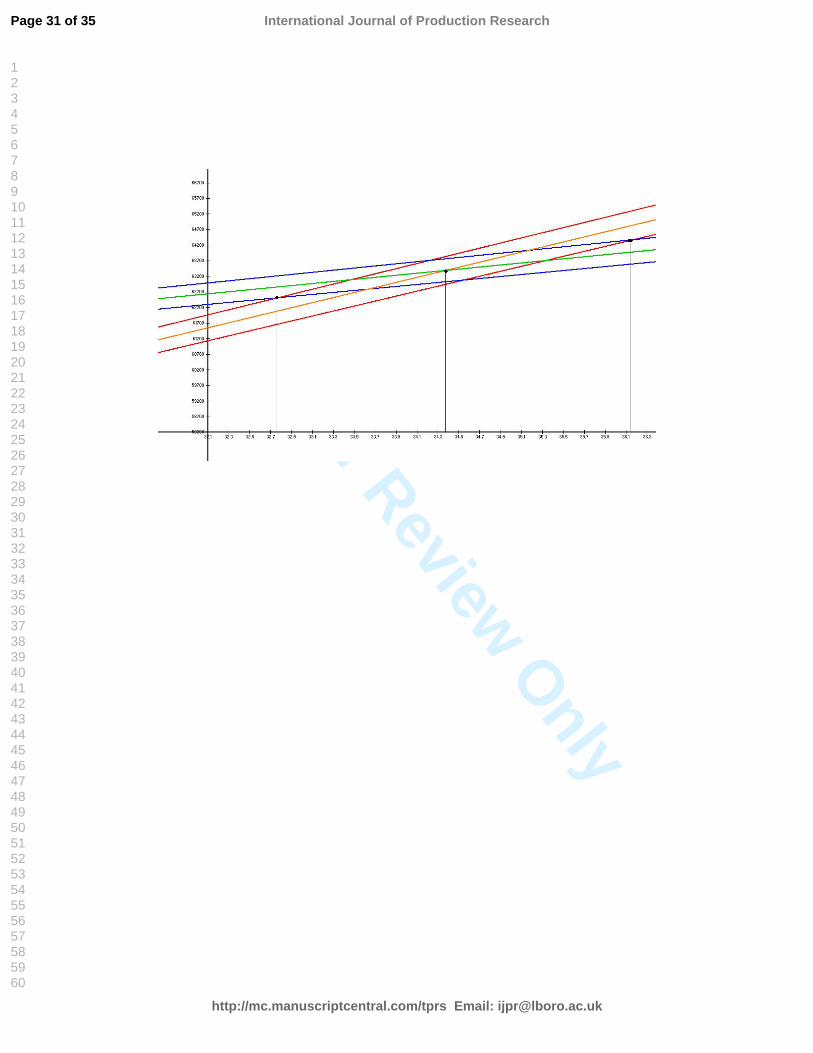
For Peer Review O
nly
n memebership grade difference D(n) = x25 0 -509023 -390977
1 -450026 0 -463384 -340616
1 -402027 0 -417745 -290255
1 -354028 0 -327106 -239894
1 -306029 0 -326467 -189533
1 -258030 0 -280828 -139172
1 -210031 0 -235189 -88811
1 -162032 0 -18955 -3845
1 -114033 0 -143911 11911
1 -66034 0 -98272 62272
1 -18035 0 -52633 112633
1 30036 0 -6993 162993
1 78037 0 38646 213354
1 126038 0 84285 263715
1 174039 0 129924 314076
1 222040 0 175363 364437
1 270041 0 221202 414798
1 318042 0 266841 465159
1 366043 0 31248 51552
1 414044 0 358119 565881
1 462045 0 403758 616242
1 510046 0 449397 666603
1 558047 0 495036 716964
1 606048 0 540675 767325
1 654049 0 586314 817686
1 702050 0 631953 868047
1 750051 0 677593 918407
1 798052 0 723232 968768
1 864053 0 768871 1019129
1 8940
Table 1 Some membership grades for different volumes
Page 35 of 35
httpmcmanuscriptcentralcomtprs Email ijprlboroacuk
International Journal of Production Research
123456789101112131415161718192021222324252627282930313233343536373839404142434445464748495051525354555657585960