COUPLING NUCLEAR INDUCED PHONON … · coupling nuclear induced phonon propagation with conversion electron mÖssbauer spectroscopy thesis michael j. parker, capt, usaf afit-enp-ms-15-j-054

COUPLING NUCLEAR INDUCED PHONON PROPAGATION WITH

CONVERSION ELECTRON MÖSSBAUER SPECTROSCOPY

THESIS

Michael J. Parker, Capt, USAF

AFIT-ENP-MS-15-J-054

DEPARTMENT OF THE AIR FORCE AIR UNIVERSITY

AIR FORCE INSTITUTE OF TECHNOLOGY

Wright-Patterson Air Force Base, Ohio

DISTRIBUTION STATEMENT A.

APPROVED FOR PUBLIC RELEASE; DISTRIBUTION UNLIMITED.

The views expressed in this thesis are those of the author and do not reflect the official

policy or position of the United States Air Force, Department of Defense, or the United

States Government. This material is declared a work of the United States Government

and is not subject to copyright protection in the United States.




THESIS

Presented to the Faculty

Department of Engineering Physics

Graduate School of Engineering and Management

Air Force Institute of Technology

Air University

Air Education and Training Command

In Partial Fulfillment of the Requirements for the

Degree of Master of Science in Nuclear Engineering

Michael J. Parker, BS

Capt, USAF

April 2015

DISTRIBUTION STATEMENT A

APPROVED FOR PUBLIC RELEASE; DISTRIBUTION UNLIMITED




Michael J. Parker, BS

Captain, USAF

Committee Membership:

Dr, Larry W. Burggraf

Chair

Maj Benjamin R. Kowash

Member

Dr. William Bailey

Member


iv

Abstract

Mössbauer spectroscopy is a very sensitive measurement technique (~10-8

eV)

which prompted motivation for the experiment described in this thesis. Namely, can a

sensitive detection system be developed to detect nuclear recoils on the order of 10 to 100

of eVs? The hypothesis that this thesis tests is: Nuclear induced phonon bursts caused by

Rutherford scattered alphas, decayed from 241

Am, in a type-310 stainless steel material

can couple with 7.3keV conversion electron Mössbauer events at the other end of the

material which will have a statistically significant effect on a Mössbauer spectrum. The

phonon bursts produced by the alpha collisions are expected to be very low energy at the

other end of length of material. Since Mössbauer spectroscopy is sensitive and can detect

the very low energy phonons, the spectrum is expected to change in at least one of the

five areas after coupling occurs: broadening in the spectrum peaks, increased/decreased

background counting rate, Mössbauer peak asymmetry, increased/decreased counting rate

under the peak, and/or a peak centroid shift. This research aims to determine the

significance of changes between spectra with phonon bursts and with no phonon bursts

through hypothesis testing, where the null hypothesis is where phonons do not affect

Mössbauer spectra in one of the five areas mentioned previously. After the spectra and

results were analyze using an f-test and t-test comparisons, this experiment failed to reject

the null result. Leading to the conclusion that additional research must be conducted.

v

Acknowledgments

First and foremost, I’d like to thank Dr. George John, a very intelligent and good

natured man. I’d also like to thank my family, Major Kowash, and Dr. Burggraf for not

giving up on me in my time of need and their support through this long, long process.

Michael J. Parker

vi

Table of Contents

Page

Abstract .............................................................................................................................. iv

Acknowledgments................................................................................................................v

Table of Contents ............................................................................................................... vi

List of Figures .................................................................................................................. viii

List of Tables ..................................................................................................................... xi

I. Introduction .....................................................................................................................1

1.1 Motivation ................................................................................................................1

1.2 Background ..............................................................................................................2 1.3 Problem Statement ...................................................................................................3

1.4 Objectives and Approach .........................................................................................4

II. Theory ............................................................................................................................5

2.1 Mössbauer Spectroscopy ..........................................................................................5

2.1.1 Overview .......................................................................................................... 5 2.1.2 Nuclear Resonance Fluorescence ................................................................... 9

2.1.3 Natural Line Width ........................................................................................ 11 2.1.4 Recoil Energy Loss ........................................................................................ 11

2.1.5 Doppler Broadening ...................................................................................... 12 2.1.6 The Mössbauer Effect .................................................................................... 14

2.1.7 Recoil-Free Emission of Gamma Rays .......................................................... 18 2.2 Phonon Sources ......................................................................................................19 2.3 Phonon Propagation ...............................................................................................21

2.3.1 Phonons and Interactions .............................................................................. 21 2.3.2 Material Properties ....................................................................................... 22

2.4 Coupling – Mössbauer Events and Phonons - Expectations ..................................23

III. Methodology and Experimental Setup ........................................................................26

3.1 Detector Design ......................................................................................................26 3.1.1 Mössbauer Technique ................................................................................... 26

3.1.2 Mössbauer Emitter ........................................................................................ 27 3.1.3 Conversion Electron Detector ....................................................................... 29 3.1.4 Mössbauer Spectrometer ............................................................................... 34 3.1.5 Material/Absorber ......................................................................................... 38 3.1.6 Phonon Source ............................................................................................... 44

vii

3.2 Experimental Runs and Descriptions ......................................................................45

3.3 Statistical Tests ......................................................................................................53 3.3.1 Curve Fitting ................................................................................................. 53 3.3.2 Statistical Hypothesis Tests ........................................................................... 54

IV. Analysis and Results ...................................................................................................57

4.1 Data Fitting ............................................................................................................57 4.2 Statistical Analysis .................................................................................................64

4.2.1 Experimental Run Analysis ............................................................................ 65 4.2.2 In-experiment Development and Variances .................................................. 74

4.2.3 Peak Asymmetry Analysis ............................................................................... 76 4.2.4 Heat Tape ...................................................................................................... 80

V. Conclusions and Recommendations ............................................................................82

5.1 Summary ................................................................................................................82 5.2 Significance of Research ........................................................................................84 5.3 Future Work ...........................................................................................................84

APPENDIX A – MATLAB Code......................................................................................86

A.1 Data Loading and Peak Fitting Parameters ............................................................86

A.2 Peak Asymmetry ....................................................................................................90 A.3 MATLAB ‘peakfit.m’ Code ...................................................................................91

Appendix B - Data ...........................................................................................................128

B.1 Voigt Fitting Results ............................................................................................128

B.2 Bootstrap Sampling Method Data ........................................................................130 B.3 Peak Asymmetry Fitting Results ..........................................................................135

Bibliography ....................................................................................................................138

viii

List of Figures

Page

Figure 1: Energy level structure of the 57Fe nucleus. Modified from [14] ..................... 7

Figure 2: Diagram of Free and Bound Nuclei. ................................................................ 8

Figure 3: Top: The nuclear decay scheme for 57

Co → 57

Fe. Modified from [4, 21]

Bottom: Probabilities of gamma and conversion electron emission following

resonant absorption. [21, 23] ....................................................................................... 9

Figure 4: Idealized representation of nuclear resonance fluorescence and natural line

width. Modified from [6] ........................................................................................... 10

Figure 5: Resonance Overlap. Note: Overlap extremely exaggerated. .......................... 13

Figure 6: Top: Example of conversion electron Mössbauer spectrometer setup with a

corresponding spectrum. Bottom: Depiction of CEMS resonance locations in the

absorber near the surface and in the bulk. ................................................................. 16

Figure 7: Formation of a Mössbauer Spectrum using CEMS, the source is moved to

Doppler shift the center. Modified from [4]. ............................................................. 17

Figure 8: Schematic of the vibrational energy levels in a solid. [17] ............................ 19

Figure 9: Differential angular cross section for Rutherford scattering in stainless steel

type 310 with an alpha particle with 5.5 MeV energy. .............................................. 20

Figure 10: Acoustic (a) transverse, (b) longitudinal motion: the atoms move together.

[26] ............................................................................................................................. 23

Figure 11: Phonon Annihilation and Creation. [26] ...................................................... 24

Figure 12: Conversion Electron Mössbauer Spectroscopy (CEMS) Experimental Setup.

Starting from the left: 57

Co source emitter attached to the oscillating motor, a lead

collimator for the 14.4 keV gammas, CE proportional gas detector attached to left

side of 1” diameter stainless steel type-310 bar, phonon source encased in a

mounting device attached to the right side of the same bar. ...................................... 27

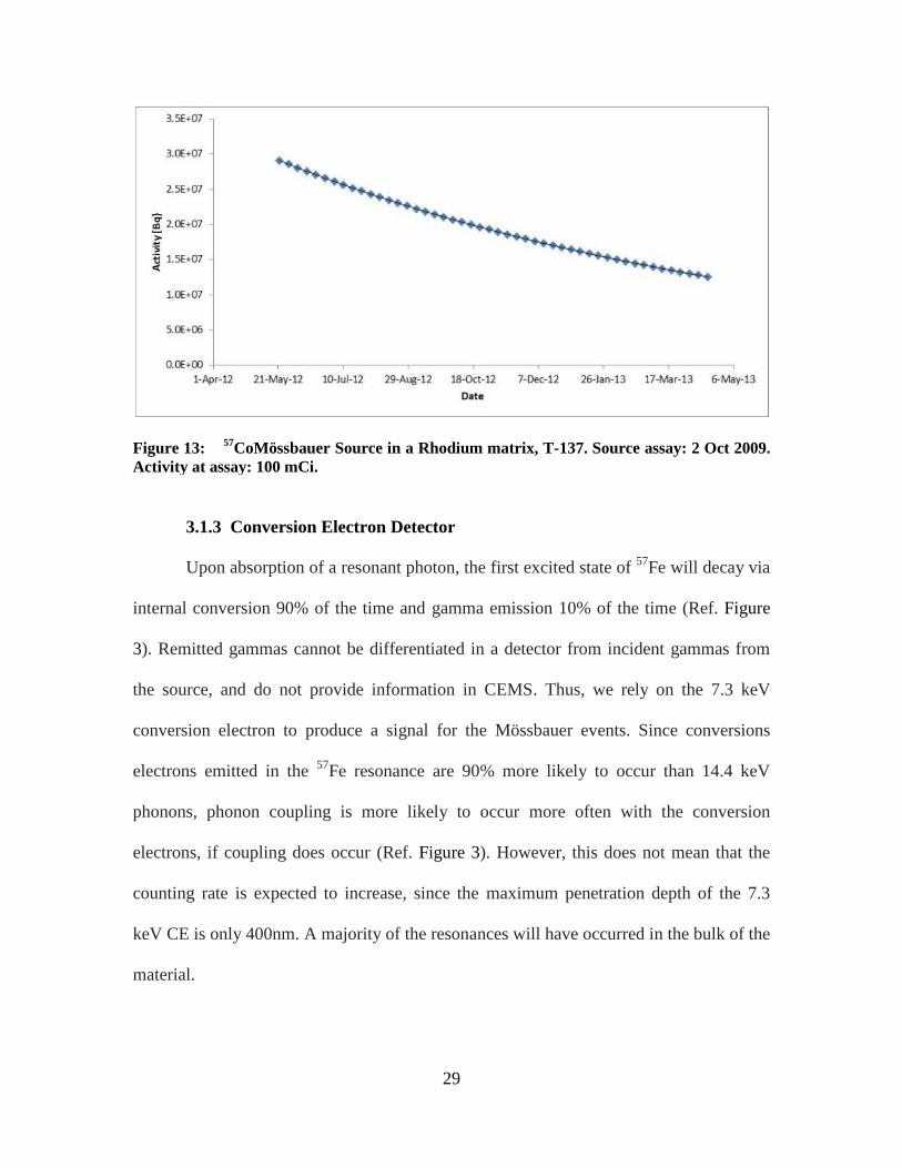
Figure 13: 57

CoMössbauer Source in a Rhodium matrix, T-137. Source assay: 2 Oct

2009. Activity at assay: 100 mCi. .............................................................................. 29

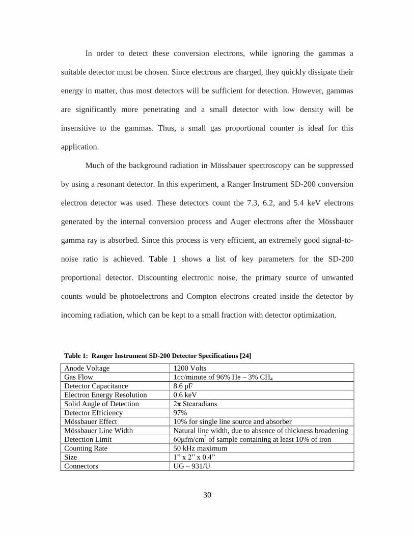
Figure 14: Simple diagram of the SD200: a gas-flow proportional detector for CEMS.

................................................................................................................................... 32

ix

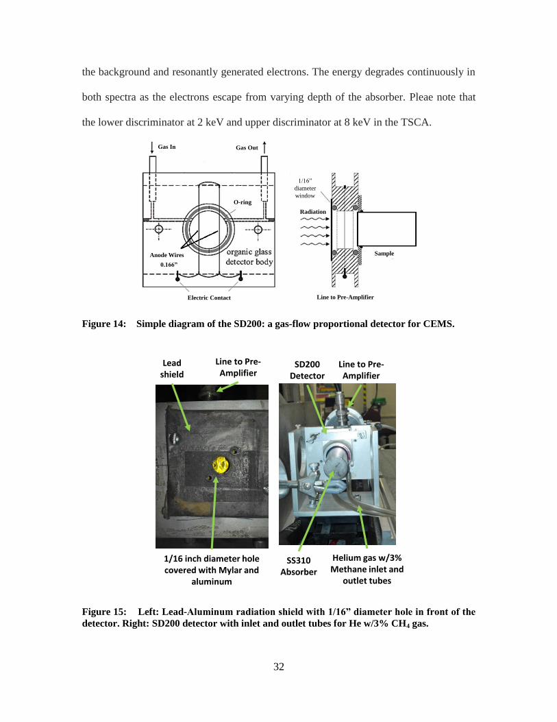
Figure 15: Left: Lead-Aluminum radiation shield with 1/16” diameter hole in front of

the detector. Right: SD200 detector with inlet and outlet tubes for He w/3% CH4 gas.

................................................................................................................................... 32

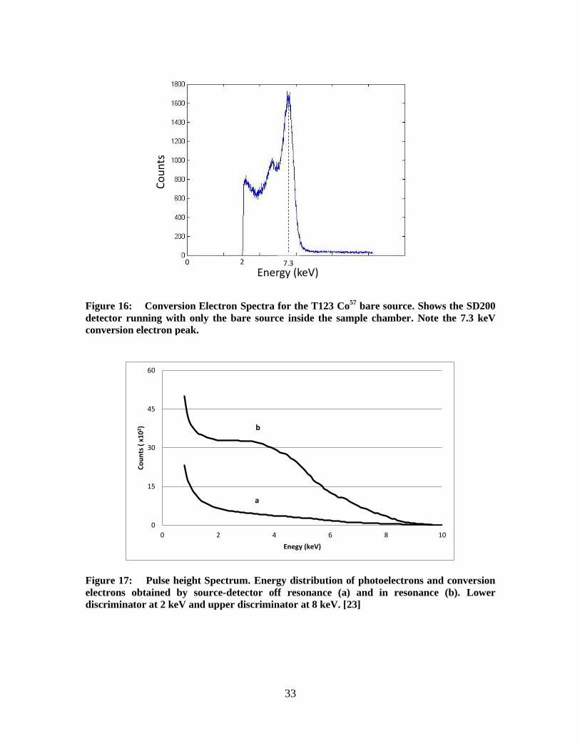
Figure 16: Conversion Electron Spectra for the T123 Co57

bare source. Shows the

SD200 detector running with only the bare source inside the sample chamber. Note

the 7.3 keV conversion electron peak. ....................................................................... 33

Figure 17: Pulse height Spectrum. Energy distribution of photoelectrons and conversion

electrons obtained by source-detector off resonance (a) and in resonance (b). Lower

discriminator at 2 keV and upper discriminator at 8 keV. [23] ................................. 33

Figure 18: Block Diagram of Mössbauer Spectrometer Electrical System ................... 35

Figure 19: (a) Triangular drive voltage. (b) A V-shaped interference fringe spectrum,

superimposed on a sextet spectrum. [1] ..................................................................... 37

Figure 20: Top: Image of the oscillating motor, laser calibration, 57

Co source location

and lead collimator. Bottom: Source orientation from detector window, SD200

detector and SS310 absorber rod. .............................................................................. 38

Figure 21: Iron-57 Mössbauer transmission spectra of (from top to bottom) α-Fe, α-

Fe2O3, γ- Fe2O3, Fe3O4 [9]. Oxidation does not change the counting rate, but does

shift and create new peaks. The iron isotope only changes the oxidation state, but not

it’s resonance cross section. ....................................................................................... 40

Figure 22: Absorber spectrum comparison. (a) Natural iron foil with a 6-day acquisition

time. (b) Enriched iron-57 feeler guage with a 2-hr acquisition time. (c) Stainless

Steel Type 310 foil with a 40-hr acquisition time. The vertical is relative counts verse

channel number/velocity. ........................................................................................... 42

Figure 23: Specifications for the absorber and the iron phonon source holder ............. 44

Figure 24: 241

Am alpha source configuration with holder and SS310 absorber rod.

Surface 1 was used for the Mössbauer event sites and surface 2 was used for the

incident alphas. (a) Button directed towards absorber surface, alphas incident. (b)

Button directed away absorber surface, alphas shielded, only gammas. ................... 47

Figure 25: Voigt, Gaussian, Lorentzian Model Fit Comparison. Top row: Run19 with

fitting errors: V-1.238%, G-1.246%, L-.234%. Bottom row: Run44I with fitting

errors: V-0.355%, G-0.371% and L-0.367%. Note the pink like is an initial estimate

of the peak location and not the actual location. ....................................................... 59

Figure 26: Iterative Fitting Errors. Typical percent parameters errors as a function of

fitting error for a simulated noisy Gaussian signal. [20] ........................................... 61

x

Figure 27: Voigt Model Fit to Run34 data. Blue dots are the measured data points, the

red line is the Voigt model fit to the data. Fit parameters are displayed in the top

subplot. The pink dotted line was the initial peak center estimate before the fit

iteration. The lower subplot below displays the residuals from the model fit. In all

cases, the mean of the residuals trended towards zero. ............................................. 63

Figure 28: Peak and background counting rate graphical comparison for 11mm/s motor

velocity. Source runs: (a) No Phonon (b) Phonon and (c) Peak vs Background trends

................................................................................................................................... 70

Figure 29: Peak and background counting rate graphical comparison for 22mm/s motor

velocity. ..................................................................................................................... 71

Figure 30: FWHM graphical comparison for 11mm/s and 22mm/s motor velocities.

Source Runs: (a) No Phonon (b) Phonon .................................................................. 72

Figure 31: Peak Development for In-Experiment Runs. Peaks are the Voigt fit to the

data. Top: Run40A-F. Bottom: Run44A-I. ................................................................ 75

xi

List of Tables

Page

Table 1: Ranger Instrument SD-200 Detector Specifications [24] .................................. 30

Table 2: Stainless Steel Type 310 Properties ................................................................... 43

Table 3: Reproducibility HV = 1250V, Doppler Motor Laser Calibration Green........... 45

Table 4: Summary of Experimental Runs Performed ...................................................... 48

Table 5: f values at the 95% Confidence Level where v1 and v2 are the degrees of

freedom (# of runs minus 1). Table used as reference point, while actual confidence

intervals calculated using Microsoft Excel. ............................................................... 56

Table 6: Bootstrap Data for Run34 using the Voigt model. Appendix B.2 contains

bootstrap data for other runs ...................................................................................... 62

Table 7: Statistical comparisons for phonon source and no phonon source in Figure 28,

Figure 29, and Figure 30. The f-test was the primary method used to calculate a p-

value and a confidence interval for the FWHM, the peak and background counting

rates. ........................................................................................................................... 69

Table 8: 11mm/s motor velocity run f-test p-value and confidence interval comparisons

for the FWHM, the peak and background counting rates. The two columns on the left

represents the runs that were associated with a phonon source or no phonon source.

................................................................................................................................... 73

Table 9: In-experiment peak development statistics for the 22mm/s motor velocity runs.

Parameters: mean, standard deviation (STD) and variance of each all the runs in a

set. Example: Run set 40, runs in the set A-F. ........................................................... 74

Table 10: A list of the runs that were analyzed and compared in the peak asymmetry

analysis ...................................................................................................................... 78

Table 11: Calculated f-test p-values and confidence intervals for Peak Asymmetry. Top:

Comparison of phonon source and no source for the left and right side of the peaks.

Bottom: Comparison of the left and right side of the peaks for a phonon source and

no source. For each comparison, the 11mm/s and 22mm/s motor velocity runs should

not be compared with each other. .............................................................................. 79

1



I. Introduction

1.1 Motivation

The Mössbauer effect has many different applications in a variety of areas; such

as, the demonstration of the gravitational red-shift, nuclear physics with the study gamma

decay, and solid-state physics with the study of lattice dynamics and hyperfine

interactions. Currently, the main area of focus is in the study of chemical and physical

environments of a nucleus. Due to the extreme precision and sensitivity of the effect, it

has been used as a way determining the change in energy as a photon falls in a

gravitational field. In 1964, the shift in frequency of electromagnetic radiation as it

passed through a difference in gravitational potential was measured to be 0.859 ± 0.085

times the value predicted by Einstein’s Theory of Relativity’s Principle of Equivalence

[3]. This measurement made by Cranshaw (1964), following Pound and Rebka’s 1960

ΔE/E measurements of 4.902 x 10-15

for a 45m round trip, gave increase fidelity to their

measurement. These were the most precise tests of the General Theory of Relativity, and

it would not have been possible without the great sensitivity provided by the Mössbauer

effect [12]. It is this sensitivity that gives motivation to the experiment performed and

described herein. Depending on the speed of the Mössbauer velocity drive and radiation

source, the sensitivity can be tuned to energy regimes of interest down to Γ/Eγ per

channel.

2

Solids can absorb energy in many ways other than by removing atoms from their

lattice sites. At low energies and temperatures, the primary way is through lattice

vibrations, called phonons [12]. Propagation of these phonons through a lattice is

responsible for the familiar properties such as mechanical and acoustical waves. One of

the proposals of this experiment is to detect extremely small nuclear recoils made by

radiation scattering from individual nuclei. During a scattering event the nucleus is

displaced sending phonons into the material lattice. These phonons can then

constructively and destructively interact with nuclei in the region where the resonance

measurements are being made. The result would then be a Mössbauer spectrum that is

perturbed from one where no scattering source is present.

1.2 Background

There are two broad types of Mössbauer spectroscopy that have been applied over

the past six decades: transmission Mössbauer spectroscopy (TMS) and emission

Mössbauer spectroscopy. TMS requires a thin foil of material to allow transmission of γ-

photons to a detector behind the absorber. Photons that are resonant with the absorber and

captured then fluoresce in 4π space producing dip(s) in the Mössbauer spectrum.

Conversion electron Mössbauer spectroscopy (CEMS) is a type of emission Mössbauer

spectroscopy that allows for the surface of materials to be studied. In CEMS, the

conversion electrons emitted by the resonantly excited nuclei on the surface of the

absorber are detected producing peak(s) in the Mössbauer spectrum. In both cases, the

dip(s) and peak(s) in each respective spectrum are analyzed to determine the chemical

and nuclear environment at of the material in question. CEMS is the technique that was

3

selected for this research over TMS because the thickness of the absorber can be

considered irrelevant.

CEMS only penetrates about 50 Å to 4000Å into the material and does not

consider the chemical environment beyond this local area [9, 21]. However, energy can

be transmitted through the material into the surface regime through phonons. Phonons are

quasi-particles that transfer energy through solids in a vibrational wave motion. In

essence, the nuclei vibrate and transfer energy down the line to the next nuclei. This

propagation of this vibrational energy can extend meters in distance depending on the

material structure and the initial cause of the phonon generation. These phonons can be

generated through radiation induced nuclear recoils. In this experiment, alpha particles

are used to induce these recoils and therefore generate a phonon wave that will travel

down an absorber to localized Mössbauer events at the other end of the absorber on the

surface. It is in this localized area on the surface where the sensitivity of Mössbauer

spectroscopy (down to ~10-15

eV/eV) can possibly exploit subtle perturbations in the

spectra from the phonon interactions.

1.3 Problem Statement

Nuclear induced phonons can couple with conversion electron Mössbauer events

to have a statistically significant effect changes on a Mössbauer spectrum. The spectrum

is expected to change in at least one of the four areas: broadening in the peaks,

increased/decreased background counting rate, Mössbauer peak asymmetry, and

increase/decreased counting rate under the peak. This research aims to determine

significance of changes between spectra with phonons and no phonons through

4

hypothesis testing, where the null hypothesis is where phonons do not affect Mössbauer

spectra.

1.4 Objectives and Approach

The primary objective of this thesis is to compare Mössbauer spectra that are

created in the presence of a scattering source to spectra created without a scattering

source to determine if there is a statistical difference between the two sets of spectra. This

is accomplished through the use of CEMS, an absorber of sufficient length to allow for

phonon propagation, and a radiation source that will induce the phonons through nuclear

recoils.

5

II. Theory

The theory section will cover Mössbauer spectroscopy, description of phonons,

and phonon coupling with Mössbauer events. This section is meant to create a basis for

the overall experiment, but if more detail is desired, please use the references in the back.

2.1 Mössbauer Spectroscopy

2.1.1 Overview

Just as atoms have quantized energy states, so do nuclei. Transitions between

nuclear energy levels, like atoms, can be accomplished through the emission or

absorption of photons in a resonant process. When a radioactive isotope decays by the

emission of an alpha or beta particle, the resulting nucleus is often left in an excited state,

which subsequently decays to its ground state by the emission of one or more γ-rays.

These energy levels (ground and excited) are influenced by the environment that

surrounds the nucleus; chemical, electronic and magnetic, which can shift or split these

energy levels. This ‘hyperfine splitting’ will be discussed further in section 2.1.8. These

changes in the energy levels can provide information about the atom's local environment

within a system and ought to be observed using resonance-fluorescence [12]. There are

two major obstacles in obtaining information on the atoms’ local environment: the

hyperfine interactions between the nucleus and its environment are extremely small, and

the recoil of the nucleus as the γ-ray is emitted or absorbed prevents resonance. [12] In

an example of a γ-ray emitted by an isolated isotope, the nucleus recoils, and results in a

decrease of the γ-ray’s energy, which was the difference between the excited and ground

6

states of the nucleus. Due to this recoil energy loss, the emitted γ-ray will not be absorbed

by another nucleus disallowing resonant absorption.

In 1958, Rudolf Mössbauer discovered that, in some cases, if the nucleus is tightly

bound in a crystal lattice, the whole crystal recoils rather than the individual nucleus [19].

Due to the much greater mass involved in recoil, the energy loss of the emitted γ-ray is

reduced so that the energy becomes very close to that of the difference in energy between

the nuclear energy levels; thus, making resonant absorption possible. For the discovery of

this effect, now known as the Mössbauer Effect, Mössbauer received the Nobel Prize in

1961. This discovery is the basis of Mössbauer spectroscopy, which has been used to

investigate material properties by looking at the hyperfine structure of nuclear energy

levels. The technique was also used to verify the prediction of General Relativity that the

energy of a photon is affected by a gravitational field [12].

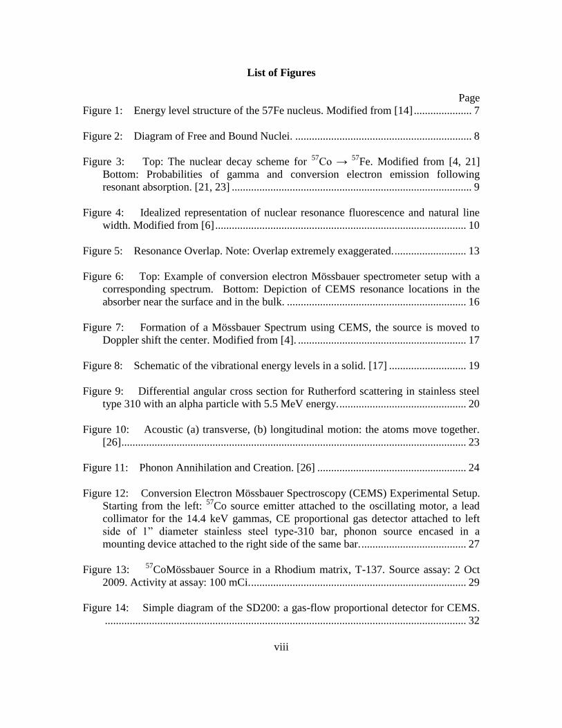
The most widely studied Mössbauer isotope is 57

Fe. The decay scheme of this

nucleus is shown in Figure 1. Radioactive decay of 57

Co by electron capture leaves the

resulting 57

Fe nucleus in an excited state. As shown in Figure 1, 9% of the excited nuclei

decay to the ground state by emitting a 137 keV γ -ray, while the remaining 91% decay in

two stages: the transition from first excited state to the second excited state emitting 123

keV γ -rays, then the transition from the second excited state to the ground state emitting

14.4 keV γ –rays. This second emission occurs with a mean lifetime of 141 ns (half life

of 97.7 ns). It is this 14.4 keV γ-ray that is frequently used in Mössbauer spectroscopy.

7

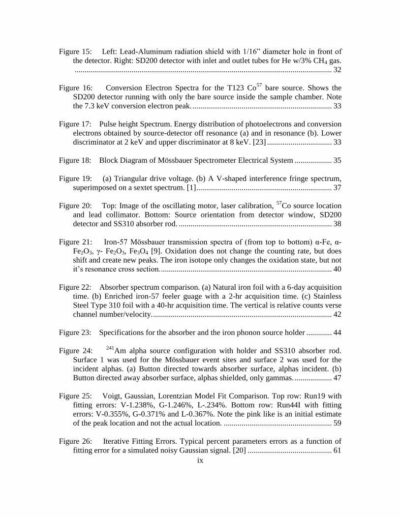
Not all resonant absorption events will be recoil free (i.e. the individual nucleus

recoils instead of the lattice). If the recoil energy is not sufficient to generate a phonon,

recoil of the individual nucleus is not possible, and the recoil momentum is taken up by

the crystal as a whole, as shown in Figure 2. The top shows the recoil of free nuclei in

emission or absorption of a γ-ray. The bottom shows recoil-free emission or absorption of

a γ-ray when the nuclei are in a solid matrix such as a crystal lattice. As a result, the

Mössbauer Effect is typically observed only for γ-rays of sufficiently low energy (5 to 50

keV), since high energy gamma rays will create larger recoils which results in a very low

recoil free fraction.

Figure 1: Energy level structure of the 57Fe nucleus. Modified from [14]

8

Figure 2: Diagram of Free and Bound Nuclei.

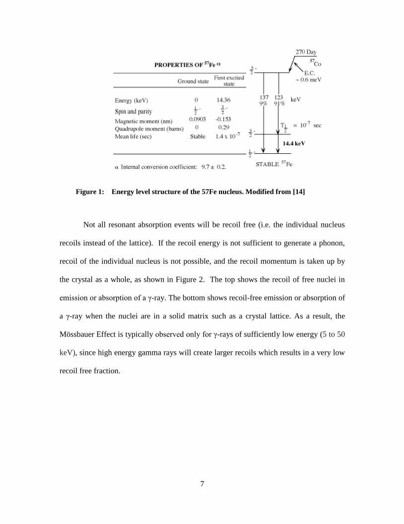
The Mössbauer effect, as generally applied to the study of minerals, relies on the

fact that 57

Fe, which is a decay product of 57

Co, is unstable. 57

Fe decays by emitting a

gamma ray (γ-ray), along with other types of radiation. Figure 3 shows the nuclear decay

scheme for 57

Co → 57

Fe and various backscattering processes for 57

Fe that can follow

resonant absorption of an incident gamma photon [6]. If a nucleus gives off radiation or

any other form of energy (in this case, in the form of a γ-ray), the nucleus must recoil (or

move) with an equal and opposite momentum to preserve its energy (Eγ), just like a gun

(by analogy, the nucleus) recoils with a recoil energy ER when firing a bullet (the γ-ray).

A more in-depth discussion of the recoil energy loss can be found in Section 2.1.4.

Eγ

m m

ER ER

E0

M M

9

Figure 3: Top: The nuclear decay scheme for 57

Co → 57

Fe. Modified from [4, 21] Bottom:

Probabilities of gamma and conversion electron emission following resonant absorption.

[21, 23]

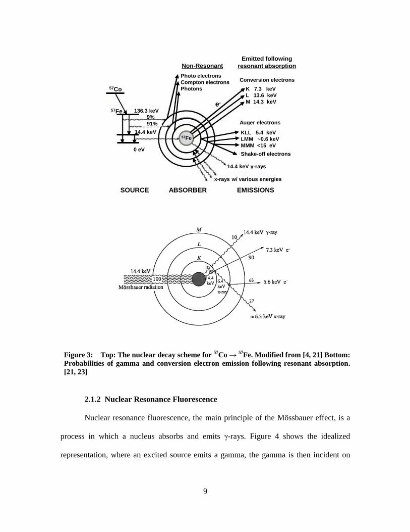
2.1.2 Nuclear Resonance Fluorescence

Nuclear resonance fluorescence, the main principle of the Mössbauer effect, is a

process in which a nucleus absorbs and emits γ-rays. Figure 4 shows the idealized

representation, where an excited source emits a gamma, the gamma is then incident on

SOURCE ABSORBER EMISSIONS

Photo electrons

Compton electrons

Photons

Conversion electrons

57Fe

57Co

57Fe

Auger electrons

KLL 5.4 keV

LMM ~0.6 keV

MMM <15 eV

Shake-off electrons

K 7.3 keV

L 13.6 keV

M 14.3 keV

x-rays w/ various energies

14.4 keV γ-rays

14.4 keV

136.3 keV9%

91%

0 eV

e-

Non-Resonant

Emitted following

resonant absorption

10

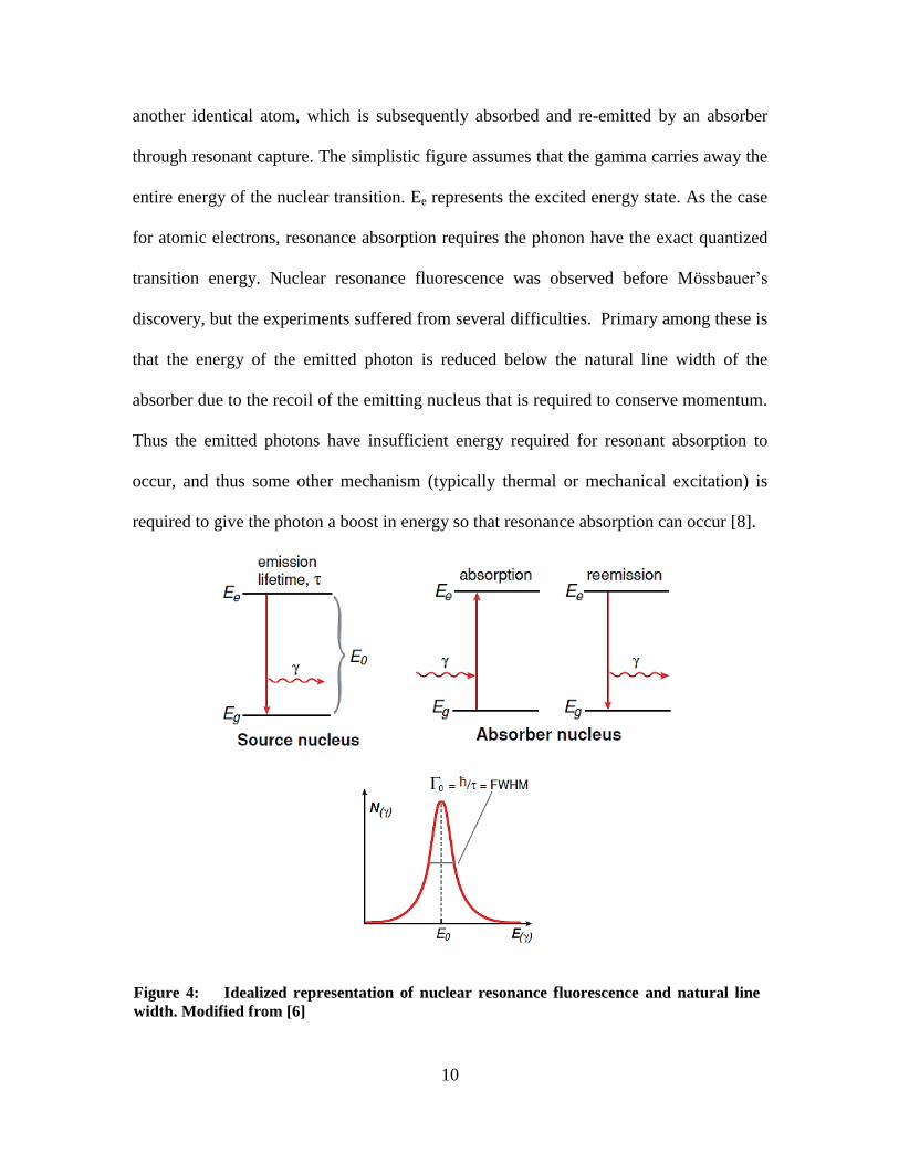
another identical atom, which is subsequently absorbed and re-emitted by an absorber

through resonant capture. The simplistic figure assumes that the gamma carries away the

entire energy of the nuclear transition. Ee represents the excited energy state. As the case

for atomic electrons, resonance absorption requires the phonon have the exact quantized

transition energy. Nuclear resonance fluorescence was observed before Mössbauer’s

discovery, but the experiments suffered from several difficulties. Primary among these is

that the energy of the emitted photon is reduced below the natural line width of the

absorber due to the recoil of the emitting nucleus that is required to conserve momentum.

Thus the emitted photons have insufficient energy required for resonant absorption to

occur, and thus some other mechanism (typically thermal or mechanical excitation) is

required to give the photon a boost in energy so that resonance absorption can occur [8].

Figure 4: Idealized representation of nuclear resonance fluorescence and natural line

width. Modified from [6]

11

2.1.3 Natural Line Width

Due to the Heisenberg uncertainty principle, the line width of the γ-ray transition

is determined by the lifetime of the first excited state which causes the energy of the

gamma to not be precisely defined. This is shown in the bottom image of Figure 4. The

profile obeys a Lorentzian (or Breit-Wigner) distribution centered on E0:

𝑓(𝐸) ∝ Γ2

Γ2+4(𝐸−𝐸0)2 (2.1)

where Γ = ℏ/𝜏, 𝜏 is the mean lifetime of the first excited state, and E0 is the energy

difference between the two levels. Emission and absorption profiles are the same.

For the 14.4 keV 57

Fe γ-ray, the mean lifetime of the first excited state is 97.7 ns

[6], corresponding to a line width Γ = 4.65x10-9

eV. Because the energy of the excited

state is not sharp, the absorption will occur even when the energies of the γ-rays differ

slightly from the resonant value. This very narrow line width makes possible Mössbauer

spectroscopy which allows the hyperfine structure of nuclear energy levels to be

investigated.

2.1.4 Recoil Energy Loss

Consider a nucleus of mass m, at rest, in an excited state of energy E0 which

decays to the ground state by emission of a γ-ray of energy Eγ, Figure 2. From

conservation of momentum and energy we find that the energy of the photon and the

energy of recoil ER are given by

Eγ = E0 - ER (2.2)

12

ER=1

2mv2=

p2

2m=

p2c2

2mc2 =Eγ

2

2mc2 (2.3)

For the 14.4 keV γ-ray emitted from 57

Fe, the recoil energy is 0.002 eV, which

greatly exceeds the width of the natural line width of 57

Fe (i.e. resonant absorption is not

possible without an additional mechanism). If the nucleus is in a crystal lattice and the

whole lattice recoils, m is replaced by the mass of the crystal, M, (M >> m), so that ER →

0 and Eγ ≈ E0. Resonant absorption is now possible. .

2.1.5 Doppler Broadening

So far in the discussion, an important factor that limits resonant absorption has

been neglected: Doppler broadening. In practice, the natural line width would not be

observed; instead the added contribution from Doppler broadening would be the primary

contributor to increased line width [12]. This broadening occurs because the nuclei of the

source and absorber are not at rest, but in fact have thermal motion at any temperature, T.

The higher the temperature, the broader the line widths become represented by ED. This

profile is presented in Figure 5.

13

Figure 5: Resonance Overlap. Note: Overlap extremely exaggerated.

In the lab frame, the emitted and absorbed photons appear Doppler shifted with

energies shown in Equation 2.4.

Eγ′ = 𝐸γ(1 ±

𝑣𝑥

𝑐) (2.4)

where, 𝑣𝑥 is the velocity component along the photon direction. The motion of the nuclei

is typically represented by the Maxwell velocity distribution with the Doppler shifted

energies. This produces a Gaussian distribution of width ED, shown in equation 2.5 and

Figure 5:

𝐸D = √ln 2 𝐸γ√2𝑘𝑇

𝑀𝑐2 (2.5)

where, kT is the thermal motion using k, Boltzmann’s constant and the temperature, T. At

room temperature kT ≈ 0.025 eV; this is on the order of magnitude of 57

Fe’s recoil

energy, ER, and produces a slight resonant overlap shown in Figure 5. It is therefore

possible (albeit with low probability) to observe some resonant absorption at room

temperature due to the Doppler broadening of the peaks. If you follow common sense, it

would be safe to assume that as the temperature of the source and absorber are lowered;

Source Absorber

14

the Doppler broadening effect would vanish, reducing the overlap to zero and making

resonant absorption impossible.

2.1.6 The Mössbauer Effect

For more in depth information, Fraunfelder [7] summarizes important early

developments and provides reprints of early works. For a more thorough description of

the theory behind Mössbauer spectroscopy, Wegener [29] is another good source. In

Mössbauer spectroscopy, an absorber material contains nuclei that are resonant with

energy emitted from a photon source. These sources and absorber nuclei are closely

coupled and are typically a parent and daughter nuclei in Mössbauer spectroscopy. The

source emits a photon at a given energy, assuming no energy loss, the absorber nuclei is

resonant with the photon and absorbs the energy of the photon. The nuclei excite and

reemit the photon’s energy in either another photon of the same energy or conversion

electrons. This process of emission, absorption and remission is called nuclear resonance

fluorescence. Unfortunately, the photon emitted by the source does lose energy through

recoil and the absorber nuclei recoils when it absorbs the photon. To overcome this

energy loss, energy is imparted to the emitted photon to allow for resonant absorption in

the absorber nuclei. This method of adding energy to the parent nuclei photon, so that the

photon carries the full transition energy is the basis of the Mössbauer effect. This method

has been used since 1958 to study hyperfine structures caused by chemical environments

of materials. Typically, the absorber materials used in the study are thin, but due to the

nature of the CEMS method, thicker materials can be used. This does not change the

spectrum generated, if the absorber is kept at room temperature (𝑇 ≈ 300𝐾).

15

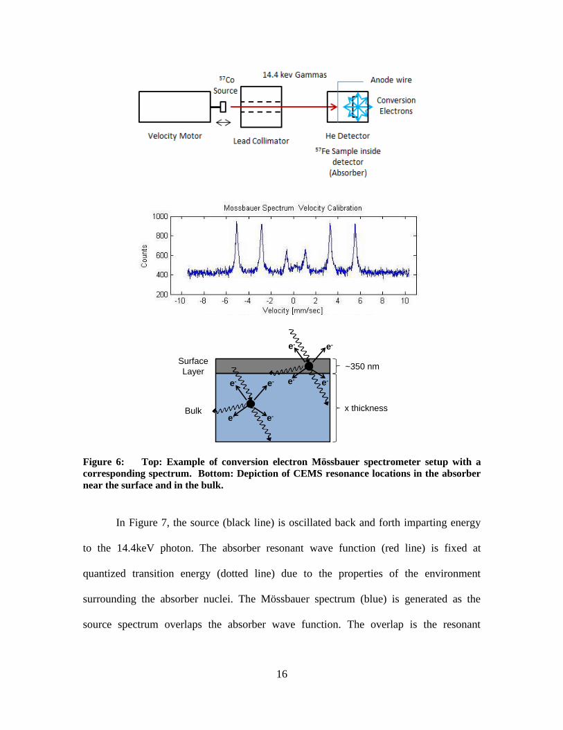
In conversation electron emission spectroscopy (CEMS), the recoil-free nuclear

resonance is the fundamental principle of Mössbauer spectroscopy where 7.3 keV

conversion electrons together with 5.4 and 6.2 keV Augur electrons are detected for 57

Fe

nuclei [21]. The CEMS technique can only occur at the surface of the absorber, as shown

in the bottom image of Figure 6. If the resonance occurs in the bulk of the absorber the

conversion electrons and Auger electrons will not be able to make it to the detector

shown in the top of Figure 6; however, if the resonance occurs on the surface layer

(400nm), which is determined by the penetration depth of the 7.3 keV conversion

elections [21]. Just as described earlier for photons, the conversion electrons that are

resonantly emitted from the 57

Fe nuclei, have the same line width as the 14.4 keV

gammas, Γ = 4.65x10-9

eV. In the spectrum shown in Figure 6, the velocity of the motor

correlates to the energy imparted on the 14.4 keV gamma, where 1 mm/s = 4.81 × 10-8

eV. So far to date, the most sensitive measurement made with Mössbauer spectroscopy

was ~10-15

eV when the gravitation shift on a photon was measured [3]. Because of the

resolution that will be used in this experiment (~10-8

eV), the setup discussed on Chapter

3 should be sensitive to shifts in energy on the same order of magnitude. The resolution

or sensitivity of the Mössbauer spectrum is dependent on the motor velocity. Increasing

motor velocity will, decrease the resolution of the spectrum, while decreasing motor

velocity will increase the resolution. The generation of the spectrum as it is dependent on

motor velocity can be seen in Figure 7.

16

Figure 6: Top: Example of conversion electron Mössbauer spectrometer setup with a

corresponding spectrum. Bottom: Depiction of CEMS resonance locations in the absorber

near the surface and in the bulk.

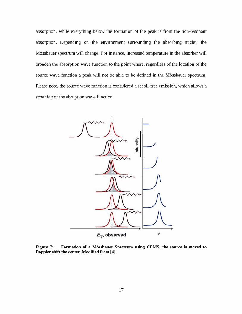
In Figure 7, the source (black line) is oscillated back and forth imparting energy

to the 14.4keV photon. The absorber resonant wave function (red line) is fixed at

quantized transition energy (dotted line) due to the properties of the environment

surrounding the absorber nuclei. The Mössbauer spectrum (blue) is generated as the

source spectrum overlaps the absorber wave function. The overlap is the resonant

Surface

Layer

Bulk

~350 nm

x thickness

e-e-

e- e-e-e-

e-e-

17

absorption, while everything below the formation of the peak is from the non-resonant

absorption. Depending on the environment surrounding the absorbing nuclei, the

Mössbauer spectrum will change. For instance, increased temperature in the absorber will

broaden the absorption wave function to the point where, regardless of the location of the

source wave function a peak will not be able to be defined in the Mössbauer spectrum.

Please note, the source wave function is considered a recoil-free emission, which allows a

scanning of the abruption wave function.

Figure 7: Formation of a Mössbauer Spectrum using CEMS, the source is moved to

Doppler shift the center. Modified from [4].

18

2.1.7 Recoil-Free Emission of Gamma Rays

To help understand recoil-free emission of gamma rays, a representational

schematic of the vibrational energy levels in a solid is shown in Figure 8. This figure

assumes an Einstein solid with a frequency, ω. Please note ℏ is Planck's constant divided

by 2π. On the left, the recoil energy ER of an emitted γ-ray is less than what is needed to

reach the next higher energy level, so that excitation of a vibrational mode has low

probability. The probability that no excitation will occur is given the symbol f, which

represents the fraction of recoil-free events, shown in equation 2.6.

𝑓 = 1 − 𝐸𝑅

ℏω (2.6)

A γ-ray would be emitted without losing energy to the solid, in what is called a

zero-phonon transition [6]. In other words, sometimes the nucleus absorbs the energy of

the γ-ray and it doesn't recoil (instead, the entire structure, rather than just the nucleus,

absorbs the energy). The variable f indicates the probability of this happening and should

be sufficiently large, 𝐸𝑅 ≫ ℏω. This process of recoil-less emission forms the basis for

Mössbauer spectroscopy. On the right, ER is significantly greater in energy than the

lowest excitation energy of the solid, which is En+1- En. Absorption of the recoil energy,

ER, by the solid thus becomes probable, and the photon emerges with energy reduced by

ER and with Doppler broadening [6].

19

Figure 8: Schematic of the vibrational energy levels in a solid. [17]

The crystal lattice does not always produce a gamma with zero recoil, if the

emitting and absorbing nuclei are in different crystal structures, the different chemical

environment is sufficient to perturb the nuclear energy levels differently so that resonant

absorption is precluded. Only a small Doppler shift in frequency, however, obtained by

moving the source, is sufficient to allow absorption by canceling out the effects of the

natural Doppler shift with the induce Doppler shift by moving the motor. The scanning

velocity of the Mössbauer photons source is the basis of Mössbauer spectroscopy, which

allows nuclear absorption spectra to be recorded. In other words, a Mössbauer spectrum

is a recoil-free resonance curve.

2.2 Phonon Sources

In this experiment, alpha particles, 4He

2+, from an Americium-241 (

241Am) source

were used to bombard the absorber and imparting energy to the absorber through

Rutherford scattering. As 241

Am decays, 5.49 MeV (85%) and 5.44 MeV (13%) alphas

are emitted. Ideally, there is no attenuation through the 241

Am source casing and microns

of air before the absorber material. A 5.49 MeV alpha has a range of about 4.05cm in dry

air at 1 atm [11]. For the theoretical section, the ideal situation is assumed. Since alpha

particles are positively charged, Rutherford scattering is the mechanism in which the

20

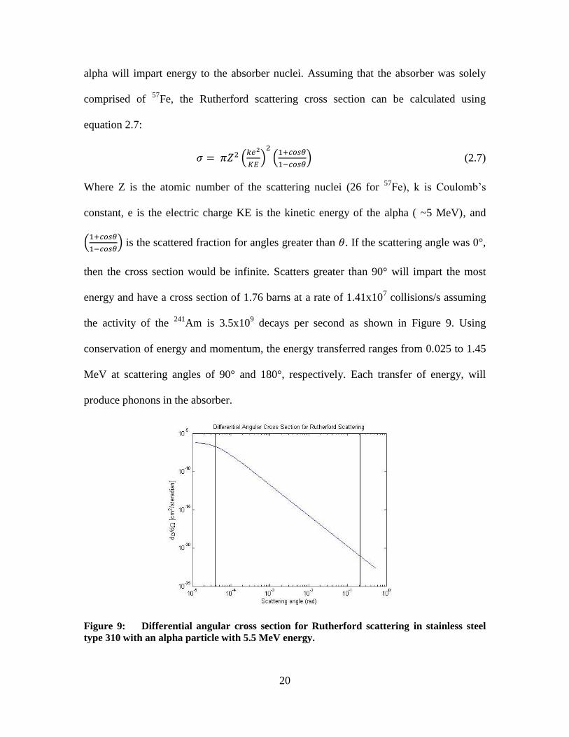
alpha will impart energy to the absorber nuclei. Assuming that the absorber was solely

comprised of 57

Fe, the Rutherford scattering cross section can be calculated using

equation 2.7:

𝜎 = 𝜋𝑍2 (𝑘𝑒2

𝐾𝐸)

2

(1+𝑐𝑜𝑠𝜃

1−𝑐𝑜𝑠𝜃) (2.7)

Where Z is the atomic number of the scattering nuclei (26 for 57

Fe), k is Coulomb’s

constant, e is the electric charge KE is the kinetic energy of the alpha ( ~5 MeV), and

(1+𝑐𝑜𝑠𝜃

1−𝑐𝑜𝑠𝜃) is the scattered fraction for angles greater than 𝜃. If the scattering angle was 0°,

then the cross section would be infinite. Scatters greater than 90° will impart the most

energy and have a cross section of 1.76 barns at a rate of 1.41x107 collisions/s assuming

the activity of the 241

Am is 3.5x109 decays per second as shown in Figure 9. Using

conservation of energy and momentum, the energy transferred ranges from 0.025 to 1.45

MeV at scattering angles of 90° and 180°, respectively. Each transfer of energy, will

produce phonons in the absorber.

Figure 9: Differential angular cross section for Rutherford scattering in stainless steel

type 310 with an alpha particle with 5.5 MeV energy.

21

2.3 Phonon Propagation

It is known that thermal spikes associated with the energy deposition events can

produce acoustic waves in the source and surrounding materials. Since more than 95% of the

energies released from radioactive decays are dissipated through atomic lattice vibrations,

acoustic waves generated by the fission products and fragments can potentially be used as

acoustic signatures for the radiation detection. The energies required to displace an atom in

solids are normally on the order of tens of electron volts, which are significantly lower than

kinetic energies of most energetic particles (e.g., about 5 MeV for an alpha particle).

Therefore, cascades of atomic displacements up to tens of micrometers are observed for

fission products and alpha decays in most solids. The highly localized deposition of energy,

which causes fast melting along the particle track, followed by recrystallization or

amorphization after the impact, can be described by the thermal spike model proposed by

Seitz and Koehler [9, 22]. They suggested that the main result of the passage of the heavy

atom through the solid is the development of highly concentrated lattice vibrations along the

trajectory, phonons.

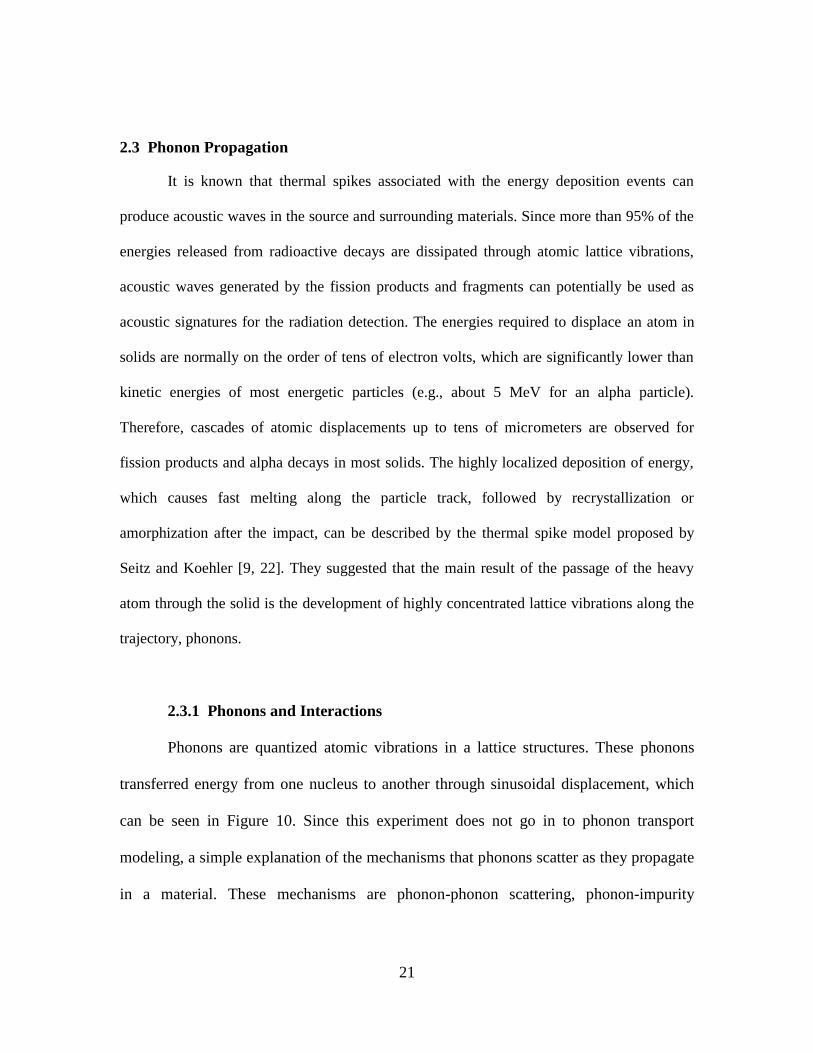
2.3.1 Phonons and Interactions

Phonons are quantized atomic vibrations in a lattice structures. These phonons

transferred energy from one nucleus to another through sinusoidal displacement, which

can be seen in Figure 10. Since this experiment does not go in to phonon transport

modeling, a simple explanation of the mechanisms that phonons scatter as they propagate

in a material. These mechanisms are phonon-phonon scattering, phonon-impurity

22

scattering, phonon-electron scattering, and phonon-boundary scattering. Each scattering

mechanism affects the normal phonon wave vector dissipating the phonon energy as

propagation occurs. As phonons scatter, their energy dissipates. Ideally, the scattering of

the phonons would be reduced with a pure crystal lattice allowing for a propagation

vector to be preserved with minimal scattering. Unfortunately, a pure crystal was not

practical for this current experiment and a material with 57

Fe was required.

2.3.2 Material Properties

The energy deposition from the Rutherford scattered alpha particles in localized

areas produce acoustic waves, which can also be described as phonons. As the distance

from the energy deposition location is increased, the energy of the phonons decay. The

properties of a material paly a large part in phonon propagation as discussed above. One

property of a material is the stiffness, which is a property of a metal, which gives it the

ability to resist being permanently, deformed. As the stiffness of a material increases,

large Young’s modulus (Y) and low density (ρ), the speed of sound will increase, as

shown in equation 2.8.

𝑎1 = √𝑌𝜌⁄ (2.8)

This allows for a faster acoustic wave in the material which can transfer the

phonon energy to the Mössbauer event sites. The absorber used in this experiment is

stainless steel Type-310, austenitic steel with 2% 57

Fe and a predicted average counting

rate of 0.604 Mössbauer events/s. Austenitic steels have austenite as their primary phase

(face centered cubic crystal). These alloys are annealed to produce a recrystallized

microstructure with a uniform grain size. The grain boundaries cannot be eliminated from

http://en.wikipedia.org/wiki/Steel

http://en.wikipedia.org/wiki/Austenite

http://en.wikipedia.org/wiki/Face_centered_cubic

23

the material and will be a cause of the decay of the phonon propagation in the

experiment.

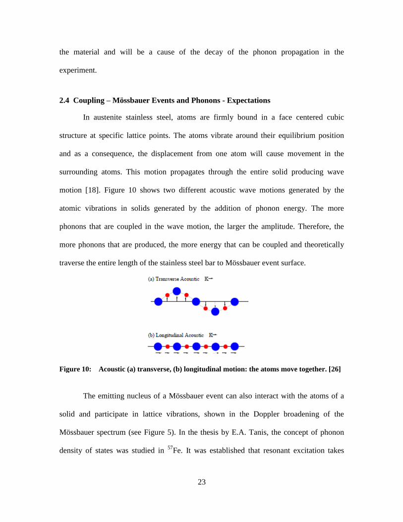
2.4 Coupling – Mössbauer Events and Phonons - Expectations

In austenite stainless steel, atoms are firmly bound in a face centered cubic

structure at specific lattice points. The atoms vibrate around their equilibrium position

and as a consequence, the displacement from one atom will cause movement in the

surrounding atoms. This motion propagates through the entire solid producing wave

motion [18]. Figure 10 shows two different acoustic wave motions generated by the

atomic vibrations in solids generated by the addition of phonon energy. The more

phonons that are coupled in the wave motion, the larger the amplitude. Therefore, the

more phonons that are produced, the more energy that can be coupled and theoretically

traverse the entire length of the stainless steel bar to Mössbauer event surface.

Figure 10: Acoustic (a) transverse, (b) longitudinal motion: the atoms move together. [26]

The emitting nucleus of a Mössbauer event can also interact with the atoms of a

solid and participate in lattice vibrations, shown in the Doppler broadening of the

Mössbauer spectrum (see Figure 5). In the thesis by E.A. Tanis, the concept of phonon

density of states was studied in 57

Fe. It was established that resonant excitation takes

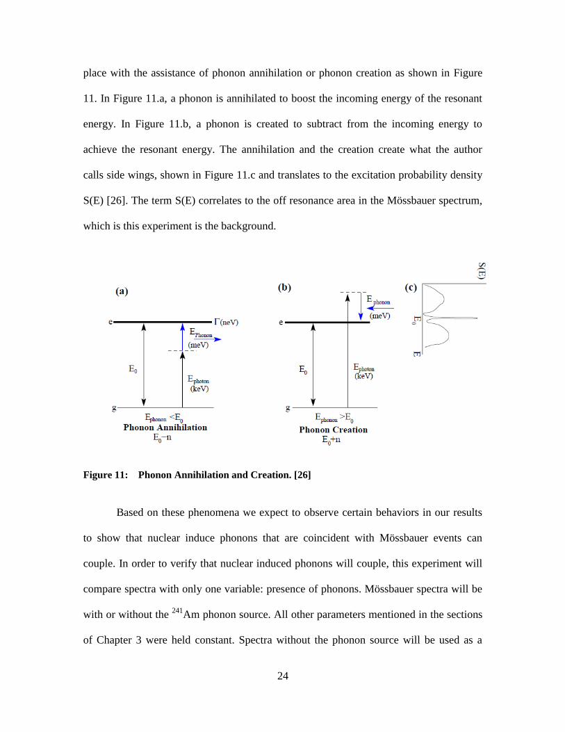
24

place with the assistance of phonon annihilation or phonon creation as shown in Figure

11. In Figure 11.a, a phonon is annihilated to boost the incoming energy of the resonant

energy. In Figure 11.b, a phonon is created to subtract from the incoming energy to

achieve the resonant energy. The annihilation and the creation create what the author

calls side wings, shown in Figure 11.c and translates to the excitation probability density

S(E) [26]. The term S(E) correlates to the off resonance area in the Mössbauer spectrum,

which is this experiment is the background.

Figure 11: Phonon Annihilation and Creation. [26]

Based on these phenomena we expect to observe certain behaviors in our results

to show that nuclear induce phonons that are coincident with Mössbauer events can

couple. In order to verify that nuclear induced phonons will couple, this experiment will

compare spectra with only one variable: presence of phonons. Mössbauer spectra will be

with or without the 241

Am phonon source. All other parameters mentioned in the sections

of Chapter 3 were held constant. Spectra without the phonon source will be used as a

25

control and compared with spectra with the phonon source. There are several expected

behaviors in the Mössbauer spectra with phonons. One is a broadening in the full width

half max (FWHM) and a broadening in the wings due to high momentum phonon

collisions with the Mössbauer event sites. A second possibility is that the counting rate of

the background should increase while the area under the resonant peak should decrease

due to phonon disruption of resonance sites. This is reflected physically by a change in

the recoil free fraction of the material. A reduction in in recoil free fractions, as discussed

in section 2.1.7, should reduce the peak of the spectrum, i.e. change the counting rate of

the peak and increase the counting rate of the non-resonant background. Various

statistical tests will be used to determine if there are any differences between the two

spectra in Section 3.4.

26

III. Methodology and Experimental Setup

This section is intended to give insight into the development of the experimental

set up, i.e. the reasoning behind choosing Mössbauer materials, the absorber, the detector

design, and the phonon source. It will also go into detail behind each run accomplished.

3.1 Detector Design

3.1.1 Mössbauer Technique

In order to harness the sensitivity of Mössbauer spectroscopy, while allowing for

phonons to couple with the Mössbauer events, a new detection system was designed. The

detection system used the Conversion Electron Mössbauer Spectroscopy (CEMS)

technique over traditional transmission Mössbauer spectroscopy (TMS) technique. In

CEMS, the conversion electrons are emitted at the surface of the material and detected.

Unlike TMS, CEMS does not have a dependence on the thickness of the Mössbauer

absorber. This means more material can be used to mount the alpha source at the other

end of the bar which can be seen in Figure 12. In our setup, it will be shown the large

amounts of material (thicknesses >1mm) are not required due to the relatively large

Rutherford scattering cross section for alpha particles in iron.

27

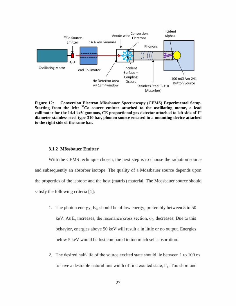
Figure 12: Conversion Electron Mössbauer Spectroscopy (CEMS) Experimental Setup.

Starting from the left: 57

Co source emitter attached to the oscillating motor, a lead

collimator for the 14.4 keV gammas, CE proportional gas detector attached to left side of 1”

diameter stainless steel type-310 bar, phonon source encased in a mounting device attached

to the right side of the same bar.

3.1.2 Mössbauer Emitter

With the CEMS technique chosen, the next step is to choose the radiation source

and subsequently an absorber isotope. The quality of a Mössbauer source depends upon

the properties of the isotope and the host (matrix) material. The Mössbauer source should

satisfy the following criteria [1]:

1. The photon energy, Eγ, should be of low energy, preferably between 5 to 50

keV. As Eγ increases, the resonance cross section, σ0, decreases. Due to this

behavior, energies above 50 keV will result a in little or no output. Energies

below 5 keV would be lost compared to too much self-absorption.

2. The desired half-life of the source excited state should lie between 1 to 100 ns

to have a desirable natural line width of first excited state, Γn. Too short and

Oscillating Motor

57Co SourceEmitter

Lead Collimator

Stainless Steel T-310(Absorber)

He Detector area w/ 1cm2 window

Anode wire

14.4 kev Gammas

Conversion Electrons

100 mCi Am-241 Button Source

Incident Alphas

Phonons

Incident Surface –Coupling Occurs

28

Γn would not allow for any hyperfine structures to be resolved. Conversely,

too long and Γn would be too narrow allowing small mechanical vibrations to

destroy the resonance condition.

3. The internal conversion coefficient, α, should be small to ensure a large γ-ray

emission from the source compared to the electron emission.

4. The source should balance high activity with a long half-life.

5. The Mössbauer isotope should not have high spin, which would produce

complicated spectra, i.e. hyperfine splitting.

6. The Mössbauer isotope should have a relatively high natural abundance that

enrichment would not be required and allow for an increased counting rate of

Mössbauer events.

Among the isotopes in which the Mössbauer effect has been observed, the 57

Co

parent in a Rhodium (Rh) matrix and 57

Fe daughter satisfies all the above requirements.

The 57

Co source produces a high recoilless fraction, has a convenient line width, and an

intense 14.4 keV γ-ray. Additionally, with a 271 day half-life and relatively low energy

gamma rays (highest energy is 136 keV), 57

Co is a convenient source to use in the

laboratory. The activity of the 57

Co source used in this experiment is shown in Figure 13.

29

Figure 13: 57

CoMössbauer Source in a Rhodium matrix, T-137. Source assay: 2 Oct 2009.

Activity at assay: 100 mCi.

3.1.3 Conversion Electron Detector

Upon absorption of a resonant photon, the first excited state of 57

Fe will decay via

internal conversion 90% of the time and gamma emission 10% of the time (Ref. Figure

3). Remitted gammas cannot be differentiated in a detector from incident gammas from

the source, and do not provide information in CEMS. Thus, we rely on the 7.3 keV

conversion electron to produce a signal for the Mössbauer events. Since conversions

electrons emitted in the 57

Fe resonance are 90% more likely to occur than 14.4 keV

phonons, phonon coupling is more likely to occur more often with the conversion

electrons, if coupling does occur (Ref. Figure 3). However, this does not mean that the

counting rate is expected to increase, since the maximum penetration depth of the 7.3

keV CE is only 400nm. A majority of the resonances will have occurred in the bulk of the

material.

30

In order to detect these conversion electrons, while ignoring the gammas a

suitable detector must be chosen. Since electrons are charged, they quickly dissipate their

energy in matter, thus most detectors will be sufficient for detection. However, gammas

are significantly more penetrating and a small detector with low density will be

insensitive to the gammas. Thus, a small gas proportional counter is ideal for this

application.

Much of the background radiation in Mössbauer spectroscopy can be suppressed

by using a resonant detector. In this experiment, a Ranger Instrument SD-200 conversion

electron detector was used. These detectors count the 7.3, 6.2, and 5.4 keV electrons

generated by the internal conversion process and Auger electrons after the Mössbauer

gamma ray is absorbed. Since this process is very efficient, an extremely good signal-to-

noise ratio is achieved. Table 1 shows a list of key parameters for the SD-200

proportional detector. Discounting electronic noise, the primary source of unwanted

counts would be photoelectrons and Compton electrons created inside the detector by

incoming radiation, which can be kept to a small fraction with detector optimization.

Table 1: Ranger Instrument SD-200 Detector Specifications [24]

Anode Voltage 1200 Volts

Gas Flow 1cc/minute of 96% He – 3% CH4

Detector Capacitance 8.6 pF

Electron Energy Resolution 0.6 keV

Solid Angle of Detection 2π Stearadians

Detector Efficiency 97%

Mössbauer Effect 10% for single line source and absorber

Mössbauer Line Width Natural line width, due to absence of thickness broadening

Detection Limit 60μfm/cm2 of sample containing at least 10% of iron

Counting Rate 50 kHz maximum

Size 1” x 2” x 0.4”

Connectors UG – 931/U

31

For Compton and photoelectric effects, Helium filled proportional counters have a

low background, are insensitive to x-ray radiation and are very efficient in detecting low

energy electrons. The SD-200 an aluminum rectangular box with two wires spaced 0.166

inches apart, as notionally shown in Figure 14. During the operation of the dual wire

detector, the anodes are kept at 1200V to remain in the proportional region for the SD-

200 configuration. As shown in the right side of Figure 15, there is an inlet and outlet tub

to allow the air to be purged of air and a constant flow of Helium gas quenched with 3%

Methane at approximately 1 cm3/s. The counter has two ½ inch windows. The front

window is covered with aluminum foil and yellow Mylar tape to allow incident gammas

from the Mössbauer source. A lead-aluminum shield was place in front of the window

with a 1/16 inch diameter hole to restrict the incident radiation to the desired area of the

window, shown in the left side of Figure 15. The other window, opposite the front and on

the other side of the anode wires has a removable cover to allow for the absorber

material. A seal is created when putting the absorber into place.

In order to characterize the SD200 proportional detector, an electron spectrum of

the 57

Fe taken, using a bare 57

Co source inside the detector without a sample, as shown in

Figure 16. Since the detector us virtually invisible to the 14.4 keV gamma, spectrum

gives the SD200 response to the 7.3 keV conversion electrons emitted from the bare

source. The spectrum to the left of the peak is the Compton continuum along with Auger

electrons. Along with the bare source electron spectrum, Figure 17 shows the pulse

height spectrum of photoelectrons and conversion electrons with the source scanning at

high velocities (a) and the source at rest (b). The source at rest corresponds to the sum of

32

the background and resonantly generated electrons. The energy degrades continuously in

both spectra as the electrons escape from varying depth of the absorber. Pleae note that

the lower discriminator at 2 keV and upper discriminator at 8 keV in the TSCA.

Figure 14: Simple diagram of the SD200: a gas-flow proportional detector for CEMS.

Figure 15: Left: Lead-Aluminum radiation shield with 1/16” diameter hole in front of the

detector. Right: SD200 detector with inlet and outlet tubes for He w/3% CH4 gas.

0.166”

1/16”

diameter

window

Line to Pre-AmplifierElectric Contact

Radiation

Sample

Gas OutGas In

O-ring

Anode Wires

Line to Pre-Amplifier

SD200 Detector

Helium gas w/3% Methane inlet and

outlet tubes

SS310 Absorber

Line to Pre-Amplifier

1/16 inch diameter hole covered with Mylar and

aluminum

Lead shield

33

Figure 16: Conversion Electron Spectra for the T123 Co57

bare source. Shows the SD200

detector running with only the bare source inside the sample chamber. Note the 7.3 keV

conversion electron peak.

Figure 17: Pulse height Spectrum. Energy distribution of photoelectrons and conversion

electrons obtained by source-detector off resonance (a) and in resonance (b). Lower

discriminator at 2 keV and upper discriminator at 8 keV. [23]

Co

un

ts

0 7.32

Energy (keV)

0

15

30

45

60

0 2 4 6 8 10

Co

un

ts (

x1

02 )

Enegy (keV)

b

a

34

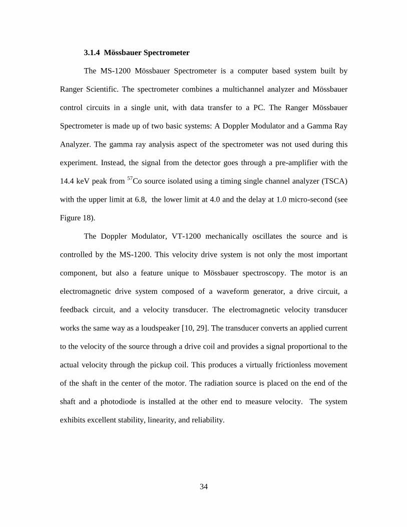
3.1.4 Mössbauer Spectrometer

The MS-1200 Mössbauer Spectrometer is a computer based system built by

Ranger Scientific. The spectrometer combines a multichannel analyzer and Mössbauer

control circuits in a single unit, with data transfer to a PC. The Ranger Mössbauer

Spectrometer is made up of two basic systems: A Doppler Modulator and a Gamma Ray

Analyzer. The gamma ray analysis aspect of the spectrometer was not used during this

experiment. Instead, the signal from the detector goes through a pre-amplifier with the

14.4 keV peak from 57

Co source isolated using a timing single channel analyzer (TSCA)

with the upper limit at 6.8, the lower limit at 4.0 and the delay at 1.0 micro-second (see

Figure 18).

The Doppler Modulator, VT-1200 mechanically oscillates the source and is

controlled by the MS-1200. This velocity drive system is not only the most important

component, but also a feature unique to Mössbauer spectroscopy. The motor is an

electromagnetic drive system composed of a waveform generator, a drive circuit, a

feedback circuit, and a velocity transducer. The electromagnetic velocity transducer

works the same way as a loudspeaker [10, 29]. The transducer converts an applied current

to the velocity of the source through a drive coil and provides a signal proportional to the

actual velocity through the pickup coil. This produces a virtually frictionless movement

of the shaft in the center of the motor. The radiation source is placed on the end of the

shaft and a photodiode is installed at the other end to measure velocity. The system

exhibits excellent stability, linearity, and reliability.

35

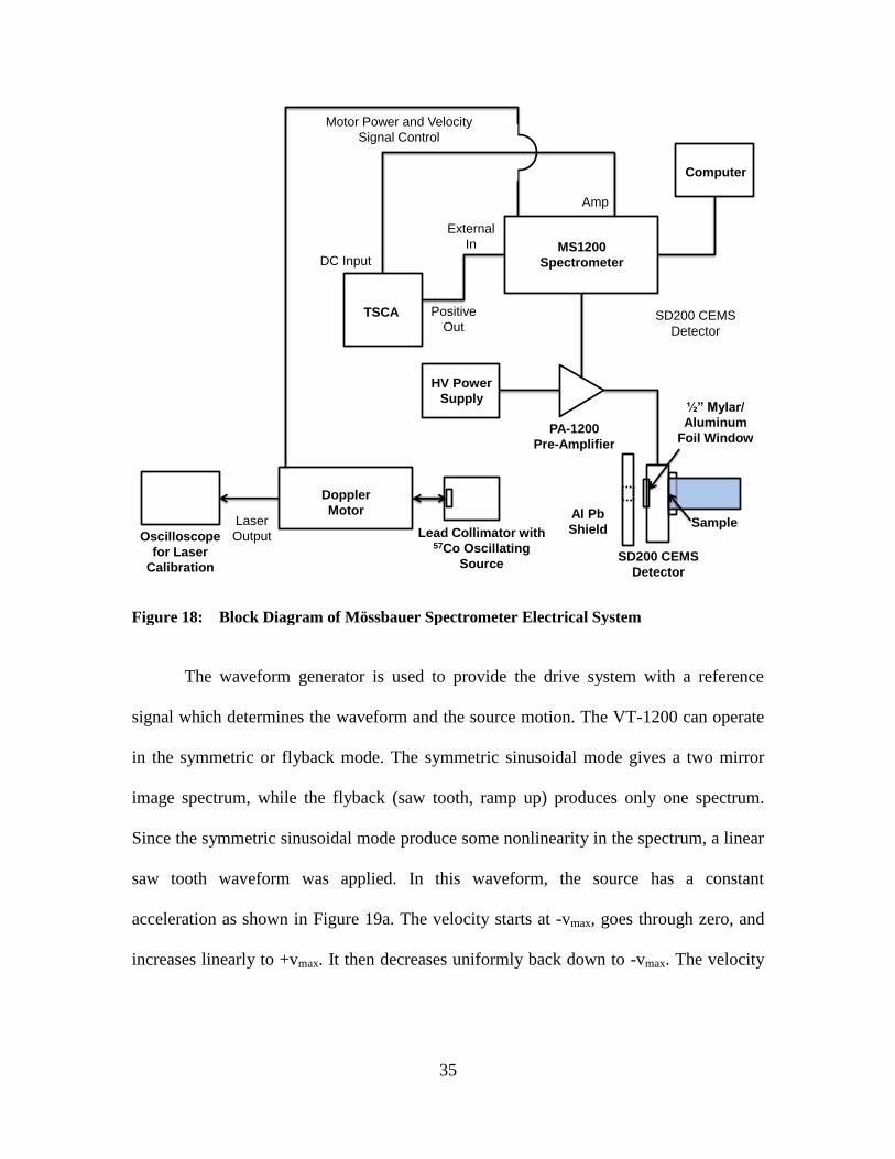
Figure 18: Block Diagram of Mössbauer Spectrometer Electrical System

The waveform generator is used to provide the drive system with a reference

signal which determines the waveform and the source motion. The VT-1200 can operate

in the symmetric or flyback mode. The symmetric sinusoidal mode gives a two mirror

image spectrum, while the flyback (saw tooth, ramp up) produces only one spectrum.

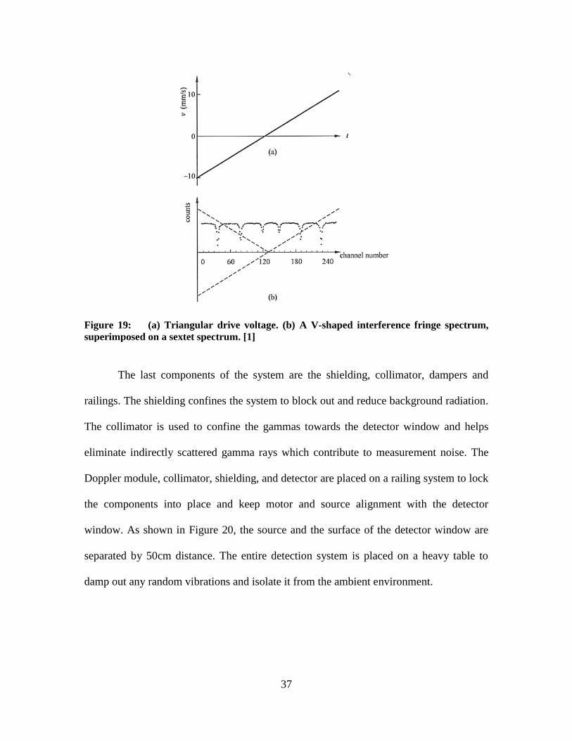
Since the symmetric sinusoidal mode produce some nonlinearity in the spectrum, a linear

saw tooth waveform was applied. In this waveform, the source has a constant

acceleration as shown in Figure 19a. The velocity starts at -vmax, goes through zero, and

increases linearly to +vmax. It then decreases uniformly back down to -vmax. The velocity

SD200 CEMS

Detector

Sample

½” Mylar/

Aluminum

Foil Window

Doppler

Motor

SD200 CEMS

Detector

Lead Collimator with57Co Oscillating

Source

Laser

OutputOscilloscope

for Laser

Calibration

PA-1200

Pre-Amplifier

HV Power

Supply

MS1200

Spectrometer

Computer

TSCA

Motor Power and Velocity

Signal Control

Positive

Out

External

In

Amp

DC Input

Al Pb

Shield

36

of the motor is in the units of mm/s and is equivalent to ΔE = 4.80766x10-8

eV. The

velocity parameter on the spectrometer was set to both ±11 mm/s and ±22 mm/s.

The system uses a laser calibration to determine the speed of the motor velocity

and velocity turn around. Since the Doppler Module is the most important part of a

Mössbauer spectrometer by adding and subtracting energy from the radiation source, it is

imperative that the motor is calibrated. This calibration assigns a velocity / energy to the

channel numbers. This is done by using laser interference fringes and Michelson patterns

to measure the absolute values of the source velocity. An oscilloscope was used to

determine the laser focus on the photodiode. These fringes are transformed by the

photodiode into pulse, which are counted by the multiscaler in the spectrometer which

produces a V-shape spectrum as seen in Figure 19b. One issue with this method is that

the fringe counts at low speeds are not as accurate, especially at zero velocity. The

maximum noise introduced into velocity spectrum is 2x10-3

mm/s. The system also has a

non-linearity less than 0.05% for the 11 mm/s velocity range [24].

37

Figure 19: (a) Triangular drive voltage. (b) A V-shaped interference fringe spectrum,

superimposed on a sextet spectrum. [1]

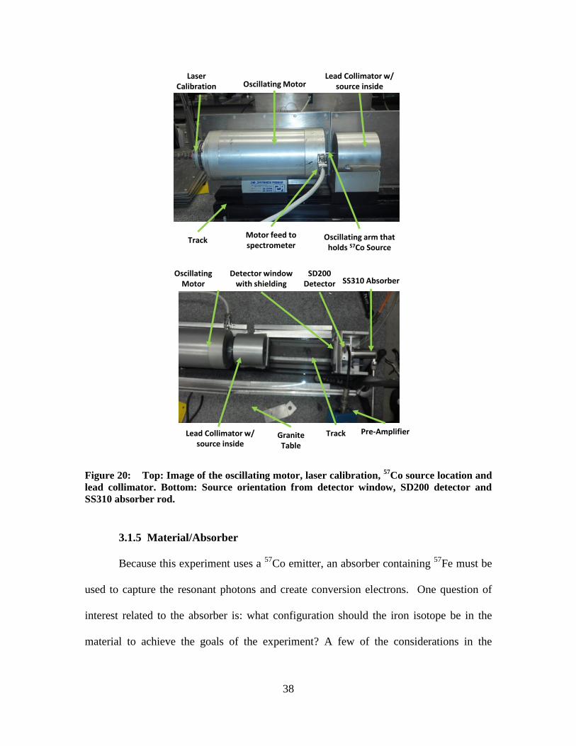
The last components of the system are the shielding, collimator, dampers and

railings. The shielding confines the system to block out and reduce background radiation.

The collimator is used to confine the gammas towards the detector window and helps

eliminate indirectly scattered gamma rays which contribute to measurement noise. The

Doppler module, collimator, shielding, and detector are placed on a railing system to lock

the components into place and keep motor and source alignment with the detector

window. As shown in Figure 20, the source and the surface of the detector window are

separated by 50cm distance. The entire detection system is placed on a heavy table to

damp out any random vibrations and isolate it from the ambient environment.

38

Figure 20: Top: Image of the oscillating motor, laser calibration, 57

Co source location and

lead collimator. Bottom: Source orientation from detector window, SD200 detector and

SS310 absorber rod.

3.1.5 Material/Absorber

Because this experiment uses a 57

Co emitter, an absorber containing 57

Fe must be

used to capture the resonant photons and create conversion electrons. One question of

interest related to the absorber is: what configuration should the iron isotope be in the

material to achieve the goals of the experiment? A few of the considerations in the

Oscillating MotorLaser

CalibrationLead Collimator w/

source inside

Oscillating arm that holds 57Co Source

Motor feed to spectrometer

Track

Oscillating Motor

SD200 Detector

Lead Collimator w/ source inside

Detector window with shielding

Pre-AmplifierTrack

SS310 Absorber

Granite Table

39

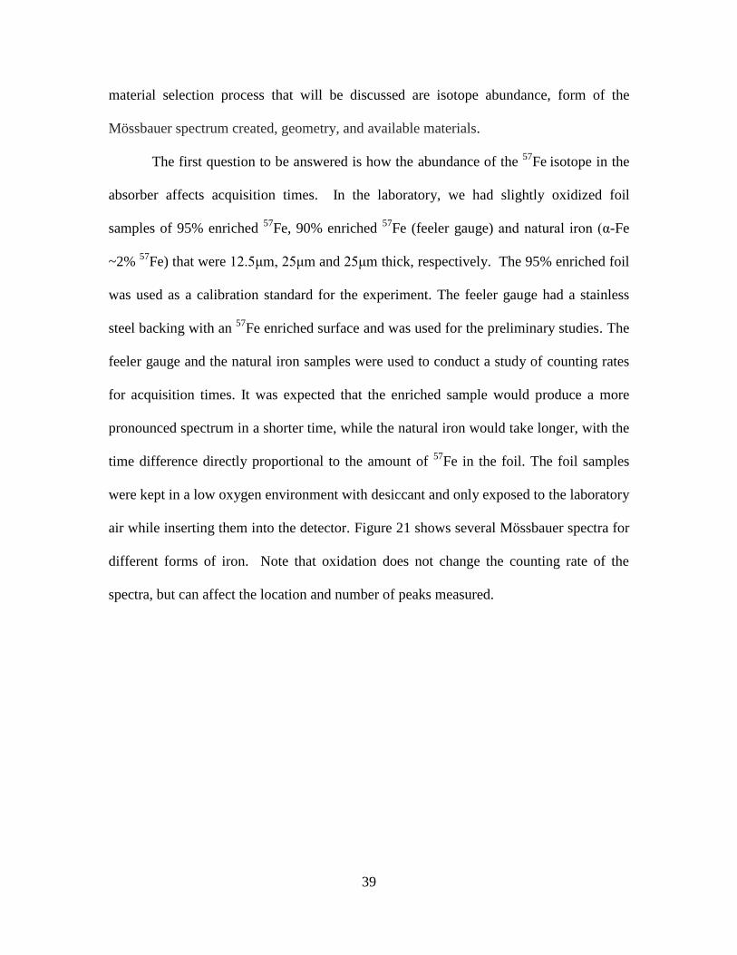
material selection process that will be discussed are isotope abundance, form of the

Mössbauer spectrum created, geometry, and available materials.

The first question to be answered is how the abundance of the 57

Fe isotope in the

absorber affects acquisition times. In the laboratory, we had slightly oxidized foil

samples of 95% enriched 57

Fe, 90% enriched 57

Fe (feeler gauge) and natural iron (α-Fe

~2% 57

Fe) that were 12.5μm, 25μm and 25μm thick, respectively. The 95% enriched foil

was used as a calibration standard for the experiment. The feeler gauge had a stainless

steel backing with an 57

Fe enriched surface and was used for the preliminary studies. The

feeler gauge and the natural iron samples were used to conduct a study of counting rates

for acquisition times. It was expected that the enriched sample would produce a more

pronounced spectrum in a shorter time, while the natural iron would take longer, with the

time difference directly proportional to the amount of 57

Fe in the foil. The foil samples

were kept in a low oxygen environment with desiccant and only exposed to the laboratory

air while inserting them into the detector. Figure 21 shows several Mössbauer spectra for

different forms of iron. Note that oxidation does not change the counting rate of the

spectra, but can affect the location and number of peaks measured.

40

Figure 21: Iron-57 Mössbauer transmission spectra of (from top to bottom) α-Fe, α-Fe2O3,

γ- Fe2O3, Fe3O4 [9]. Oxidation does not change the counting rate, but does shift and create

new peaks. The iron isotope only changes the oxidation state, but not it’s resonance cross

section.

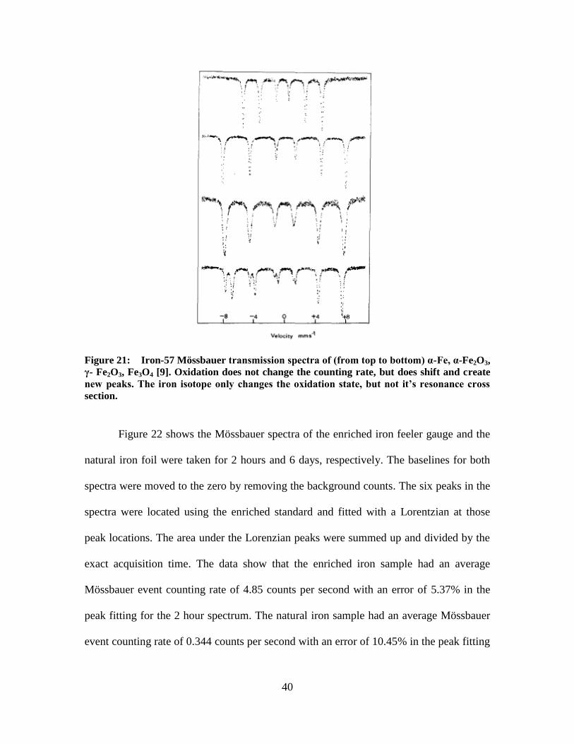
Figure 22 shows the Mössbauer spectra of the enriched iron feeler gauge and the

natural iron foil were taken for 2 hours and 6 days, respectively. The baselines for both

spectra were moved to the zero by removing the background counts. The six peaks in the

spectra were located using the enriched standard and fitted with a Lorentzian at those

peak locations. The area under the Lorenzian peaks were summed up and divided by the

exact acquisition time. The data show that the enriched iron sample had an average

Mössbauer event counting rate of 4.85 counts per second with an error of 5.37% in the

peak fitting for the 2 hour spectrum. The natural iron sample had an average Mössbauer

event counting rate of 0.344 counts per second with an error of 10.45% in the peak fitting

41

for the 6 day spectrum. Please note that the 10.45% error associated with the natural

iron sample is inconsequential to determining future acquisition times. It was evident that

using an absorber with enriched 57

Fe is preferred. Other than using the foil samples

already available in the lab, 57

Fe enrichment of an absorber was not possible due to time

and budget constraints.

Knowing that we were required to use materials with natural iron, we needed to

consider materials that would produce spectra that would be simpler to analyze. If an α-

Fe material was used, there would be six peaks to analyzed from the hyperfine structures

due to the material properties, see (a) and (b) of Figure 22. Note that in (a) the two middle

peaks were virtually useless because the peaks barely rose above the noise. This would

create a challenge to analyze. Secondly, the spectrum was acquired for 6-days and the

outside four peaks, even though they were above the noise, the signal-to-noise ratio was

only 3:2. This was after 144 hours of acquisition time. Not only are the six peaks close

enough together where they overlap slightly, there was not a large signal to noise ratio.

Considering this, a simpler spectrum needed to be analyzed.

42

Figure 22: Absorber spectrum comparison. (a) Natural iron foil with a 6-day acquisition

time. (b) Enriched iron-57 feeler guage with a 2-hr acquisition time. (c) Stainless Steel Type

310 foil with a 40-hr acquisition time. The vertical is relative counts verse channel

number/velocity.

Fortunately, literature directed the experiment to a material that would produce a

simpler spectrum, stainless steel type 310 which was available to test in the lab [Stewart,

1986]. A 25μm SS Type 310 foil sample was placed in the detector and the spectra was

acquired for 40 hours. The stainless steel sample produced only one peak that was right

of center, as seen in (c) of Figure 22. This material produced the same signal to noise

ratio for under a third of the time. Also, the sample had an average Mössbauer event

counting rate of 0.18 count/s with an error of 14.45% in the peak fitting. Even though the

counting rate was lower, it was only for one peak. Changes in the spectrum would be

easier to detect and interpret. The stainless steel type 310 properties can be seen in Table

43

2. To calibrate the stainless steel peak location, the six peaks of the enriched 57

Fe

standard was used to convert the channel numbers to velocity and energy. Section 4.1

will discuss the code that was used for the calibration.

Table 2: Stainless Steel Type 310 Properties

Composition

Fe 48.18%

(1.02% Fe57

)

C 0.25%

Cr 26%

Ni 22%

Mn 2%

Si 1.5%

P 0.05%

S 0.03%

Density 8.03 g/cm3

Elastic Modulus 200 GPa

Hardness – Rockwell B (HR B) max 95

Hardness – Brinell (HR) max 217

Number of Mössbauer Peaks 1

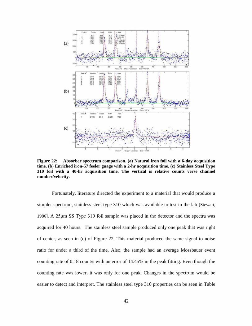
The next consideration was the geometry of the absorber. The absorber not only

had to fit in the CEMS detector opening, but had to allow a phonon inducing radiation

source to be attached at the opposite end. A 1 inch diameter cylindrical rod with two

SP12 size 118 O-rings was inserted into the CEMS detector, and the seals kept the

Helium gas from leaking. This can be seen in the right side of Figure 15. A radiation

source holder was then attached to the other side of the steel rod. The holder could

accommodate a small unsealed button source of 241

Am, and would hold it directly against

the end of the steel rod. A schematic of the rod and source holder are shown in Figure

21. The required length of the rod was unknown. To help facilitate phonon propagation

through less material, a 3 inch long rod was used and switched to a 2 inch rod later in the

experiment to help decrease distance traveled by the phonons.

44

Figure 23: Specifications for the absorber and the iron phonon source holder

3.1.6 Phonon Source

The alpha decays from 241

Am were used to produce an acoustic signal, i.e.

phonons, in the stainless steel (SS) absorber, via Rutherford scattering. The Am241

source

used for the experiment was assayed 12 Nov 1972 with a 100 mCi initial activity. Since

Am241

has a half-life of 432.6 years, the source isotropically emits 3.6x109alphas/s. The

button Am241

source was placed against the back surface of the SS rod reducing air

attenuation to virtually zero and generating a 2π Steradian solid angle. Therefore, 1.8x109

alphas/s with decay energies of 5.49 MeV (85%) and 5.44 MeV (13%) will leave the

source and be incident on the bar, after slight attenuation.

2” dia.

1” diaLoose fit for SS rod

1” 0.004” dia. Type 310 SS rod - 3 lengths: 2”, 3” and 6”

Part 1 – Type 310 Stainless Steel Rod

Part 2 – Iron Holder

> ” dia.

2” height

1”

> ”

This holds a button source

with the dimensions of

dia X . The source needs

to go into this hole loosely (i.e. it can be dropped in or the holder turned over and it falls out)

3-4 drill holes of screws to hold it onto a bar

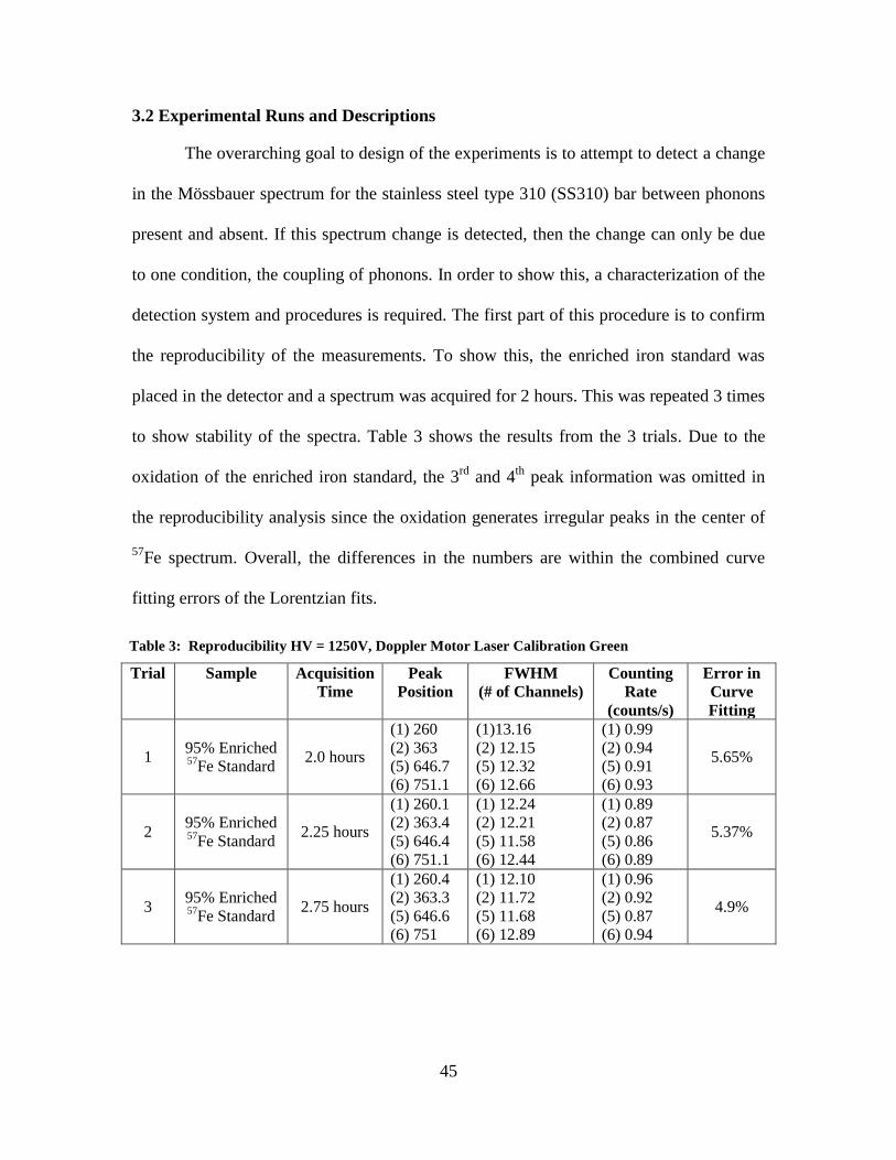
45

3.2 Experimental Runs and Descriptions

The overarching goal to design of the experiments is to attempt to detect a change

in the Mössbauer spectrum for the stainless steel type 310 (SS310) bar between phonons

present and absent. If this spectrum change is detected, then the change can only be due

to one condition, the coupling of phonons. In order to show this, a characterization of the

detection system and procedures is required. The first part of this procedure is to confirm

the reproducibility of the measurements. To show this, the enriched iron standard was

placed in the detector and a spectrum was acquired for 2 hours. This was repeated 3 times

to show stability of the spectra. Table 3 shows the results from the 3 trials. Due to the

oxidation of the enriched iron standard, the 3rd

and 4th

peak information was omitted in

the reproducibility analysis since the oxidation generates irregular peaks in the center of

57Fe spectrum. Overall, the differences in the numbers are within the combined curve

fitting errors of the Lorentzian fits.

Table 3: Reproducibility HV = 1250V, Doppler Motor Laser Calibration Green

Trial Sample Acquisition

Time

Peak

Position

FWHM

(# of Channels)

Counting

Rate

(counts/s)

Error in

Curve

Fitting

1 95% Enriched 57

Fe Standard 2.0 hours

(1) 260

(2) 363

(5) 646.7

(6) 751.1

(1)13.16

(2) 12.15

(5) 12.32

(6) 12.66

(1) 0.99

(2) 0.94

(5) 0.91

(6) 0.93

5.65%

2 95% Enriched 57


(1) 260.1

(2) 363.4

(5) 646.4

(6) 751.1

(1) 12.24

(2) 12.21

(5) 11.58

(6) 12.44

(1) 0.89

(2) 0.87

(5) 0.86

(6) 0.89

5.37%

3 95% Enriched 57


(1) 260.4

(2) 363.3

(5) 646.6

(6) 751

(1) 12.10

(2) 11.72

(5) 11.68

(6) 12.89

(1) 0.96

(2) 0.92

(5) 0.87

(6) 0.94

4.9%

46

During early phases of material selection for the absorber, a neodymium

(Nd2Fe14B) bar was considered before the SS310 bar due to the magnetic properties of

the material. The idea behind the consideration was the magnetic field would give

directionality to the phonons generated by the phonon source. At this time neutrons were

still being considered as a phonon inducing source and the boron in the material would

allow for the B(n,α)Li + 2.31 MeV reaction to produce the phonons. The bar would not

have been enriched and would contain 1.8% 57

Fe atoms (more than the SS310), but there

would have been 6 peaks for the counts to be distributed from the magnet instead of one

from the SS310 bar. When the magnet arrived in the lab, the bar has a 20μm thick nickel

coating to protect the magnet from corrosion. Instead of cutting off coating at the surface

to expose the iron in the material due to the 6 peaks, an enriched film could be attached to

the surface to help speed up acquisition times. Because of this consideration, two

additional experiments were conducted.

Since the enriched 57

Fe feeler gauge was available and only the magnetic field

was to be characterized, the feeler gauge was inserted into the detector without the

magnet first to characterize the detector. The Mössbauer spectrum was acquired for an

hour. Then, the magnetic Neodymium bar was placed with the feeler gauge sample into

the detector to characterize the effects of a magnetic field on the Mössbauer spectrum.

The sample with the bar was acquired for 1.78 hrs. After the experiment, different foils in

the lab were attached to the bar magnet. The foils bent and crumpled in the magnetic

field. It was determined that artificially enriching the surface of the bar magnet would

create discontinuity in the media and was not the best method to observe the presence of

phonons. Because of this and other reasons previously mentioned, the experiment used

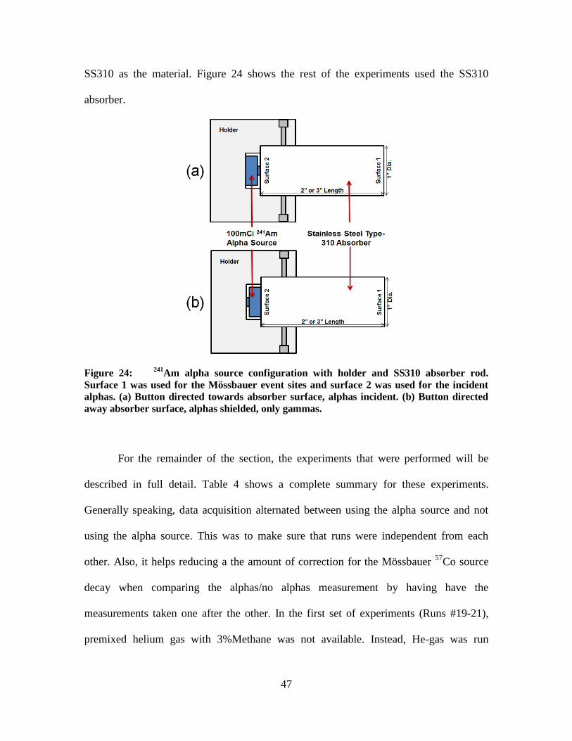
47

SS310 as the material. Figure 24 shows the rest of the experiments used the SS310

absorber.

Figure 24: 241

Am alpha source configuration with holder and SS310 absorber rod.

Surface 1 was used for the Mössbauer event sites and surface 2 was used for the incident

alphas. (a) Button directed towards absorber surface, alphas incident. (b) Button directed

away absorber surface, alphas shielded, only gammas.

For the remainder of the section, the experiments that were performed will be

described in full detail. Table 4 shows a complete summary for these experiments.

Generally speaking, data acquisition alternated between using the alpha source and not

using the alpha source. This was to make sure that runs were independent from each

other. Also, it helps reducing a the amount of correction for the Mössbauer 57

Co source

decay when comparing the alphas/no alphas measurement by having have the

measurements taken one after the other. In the first set of experiments (Runs #19-21),

premixed helium gas with 3%Methane was not available. Instead, He-gas was run

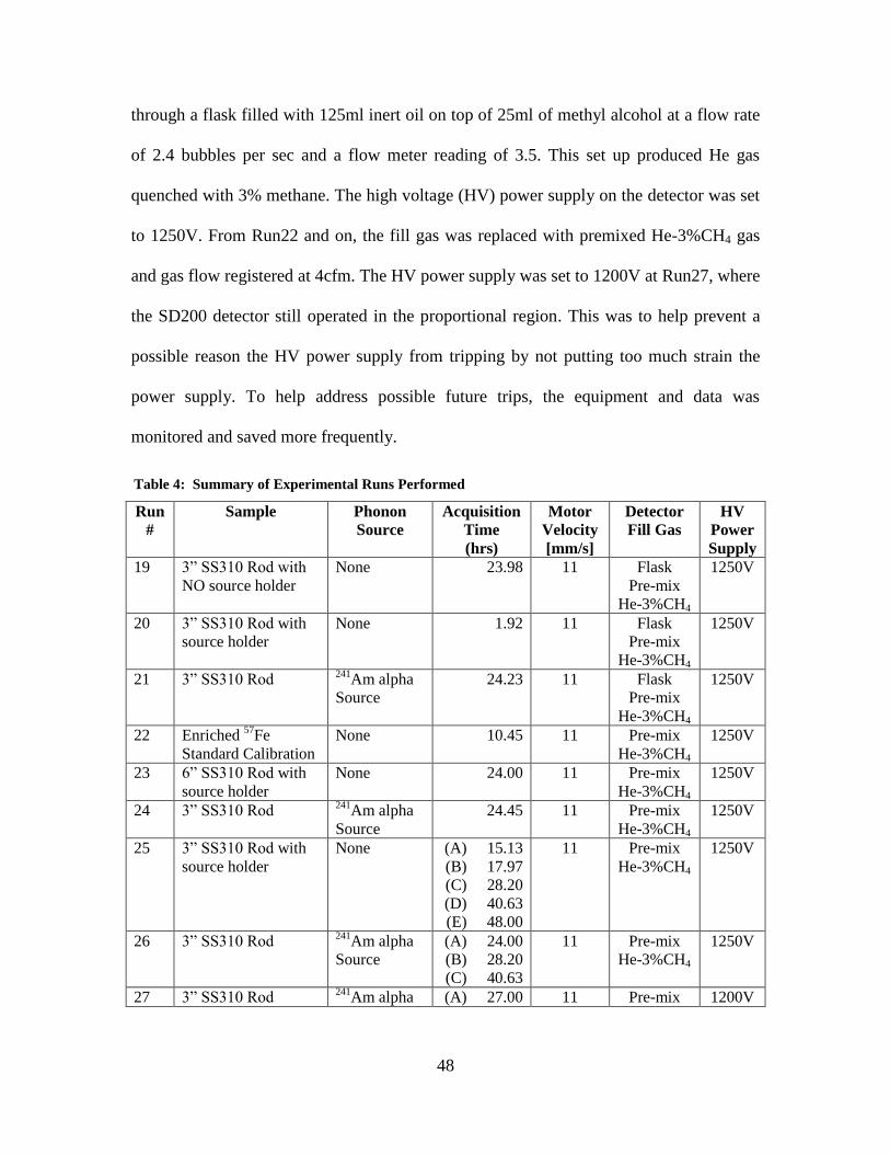
48

through a flask filled with 125ml inert oil on top of 25ml of methyl alcohol at a flow rate

of 2.4 bubbles per sec and a flow meter reading of 3.5. This set up produced He gas

quenched with 3% methane. The high voltage (HV) power supply on the detector was set

to 1250V. From Run22 and on, the fill gas was replaced with premixed He-3%CH4 gas

and gas flow registered at 4cfm. The HV power supply was set to 1200V at Run27, where

the SD200 detector still operated in the proportional region. This was to help prevent a

possible reason the HV power supply from tripping by not putting too much strain the

power supply. To help address possible future trips, the equipment and data was

monitored and saved more frequently.

Table 4: Summary of Experimental Runs Performed

Run

#

Sample Phonon

Source

Acquisition

Time

(hrs)

Motor

Velocity

[mm/s]

Detector

Fill Gas

HV

Power

Supply

19 3” SS310 Rod with

NO source holder

None 23.98 11 Flask

Pre-mix

He-3%CH4

1250V


source holder

None 1.92 11 Flask

Pre-mix

He-3%CH4

1250V

21 3” SS310 Rod 241

Am alpha

Source

24.23 11 Flask

Pre-mix

He-3%CH4

1250V

22 Enriched 57

Fe

Standard Calibration

None 10.45 11 Pre-mix

He-3%CH4

1250V


source holder


He-3%CH4

1250V

24 3” SS310 Rod 241

Am alpha

Source

24.45 11 Pre-mix

He-3%CH4

1250V


source holder

None (A) 15.13

(B) 17.97

(C) 28.20

(D) 40.63

(E) 48.00

11 Pre-mix

He-3%CH4

1250V

26 3” SS310 Rod 241

Am alpha

Source

(A) 24.00

(B) 28.20

(C) 40.63

11 Pre-mix

He-3%CH4

1250V

27 3” SS310 Rod 241

Am alpha (A) 27.00 11 Pre-mix 1200V

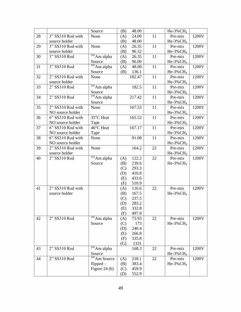
49

Source (B) 48.00 He-3%CH4


source holder

None (A) 24.00

(B) 48.00

11 Pre-mix

He-3%CH4

1200V


source holder

None (A) 26.35

(B) 96.32

11 Pre-mix

He-3%CH4

1200V

30 3” SS310 Rod 241

Am alpha

Source

(A) 26.35

(B) 96.00

11 Pre-mix

He-3%CH4

1200V

31 3” SS310 Rod 241

Am alpha

Source

(A) 48.08

(B) 136.1

11 Pre-mix

He-3%CH4

1200V


source holder


He-3%CH4

1200V

33 2” SS310 Rod 241

Am alpha

Source

182.5 11 Pre-mix

He-3%CH4

1200V

34 2” SS310 Rod 241

Am alpha

Source

217.42 11 Pre-mix

He-3%CH4

1200V


NO source holder


He-3%CH4

1200V


NO source holder

35°C Heat

Tape

165.52 11 Pre-mix

He-3%CH4

1200V


NO source holder

46°C Heat

Tape

167.17 11 Pre-mix

He-3%CH4

1200V


NO source holder


He-3%CH4

1200V


source holder


He-3%CH4

1200V

40 2” SS310 Rod 241

Am alpha

Source

(A) 122.2

(B) 239.6

(C) 293.3

(D) 410.8

(E) 433.6

(F) 510.9

22 Pre-mix

He-3%CH4

1200V


source holder

(A) 116.6

(B) 167.5

(C) 237.5

(D) 283.2

(E) 332.8

(F) 497.8

22 Pre-mix

He-3%CH4

1200V

42 2” SS310 Rod 241

Am alpha

Source

(A) 73.93

(C) 173

(D) 240.4

(E) 266.8

(F) 335.8

(G) 1331

22 Pre-mix

He-3%CH4

1200V

43 2” SS310 Rod 241

Am alpha

Source

168.3 22 Pre-mix

He-3%CH4

1200V

44 2” SS310 Rod 241

Am Source

flipped –

Figure 24 (b)

(A) 218.1

(B) 383.4

(C) 459.9

(D) 552.9

22 Pre-mix

He-3%CH4

1200V

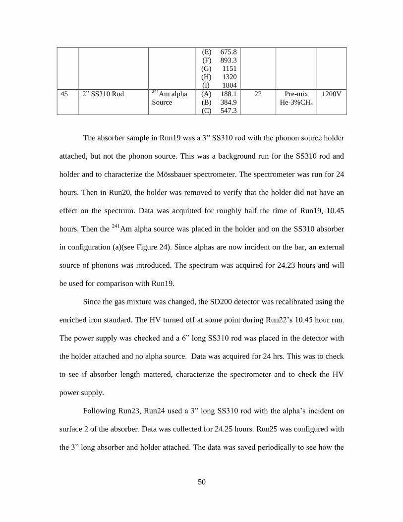
50

(E) 675.8

(F) 893.3

(G) 1151

(H) 1320

(I) 1804

45 2” SS310 Rod 241

Am alpha

Source

(A) 188.1

(B) 384.9

(C) 547.3

22 Pre-mix

He-3%CH4

1200V

The absorber sample in Run19 was a 3” SS310 rod with the phonon source holder

attached, but not the phonon source. This was a background run for the SS310 rod and

holder and to characterize the Mössbauer spectrometer. The spectrometer was run for 24

hours. Then in Run20, the holder was removed to verify that the holder did not have an

effect on the spectrum. Data was acquitted for roughly half the time of Run19, 10.45

hours. Then the 241

Am alpha source was placed in the holder and on the SS310 absorber

in configuration (a)(see Figure 24). Since alphas are now incident on the bar, an external

source of phonons was introduced. The spectrum was acquired for 24.23 hours and will

be used for comparison with Run19.

Since the gas mixture was changed, the SD200 detector was recalibrated using the

enriched iron standard. The HV turned off at some point during Run22’s 10.45 hour run.

The power supply was checked and a 6” long SS310 rod was placed in the detector with

the holder attached and no alpha source. Data was acquired for 24 hrs. This was to check

to see if absorber length mattered, characterize the spectrometer and to check the HV

power supply.

Following Run23, Run24 used a 3” long SS310 rod with the alpha’s incident on

surface 2 of the absorber. Data was collected for 24.25 hours. Run25 was configured with

the 3” long absorber and holder attached. The data was saved periodically to see how the

51

spectra changed and gather more data sets for future analysis. During this run, the HV

power supply tripped at some point between Run25A and Run25B. The alpha source was

placed back into the holder for Run26. At some point during Run26B and Run26C the

power supply turned off again. To help mitigate the problem, the HV power supply was

changed from 1250V to 1200V.

The alpha source remained in the holder for Run27 and data was acquired for 27

and 48 hrs. Then the alpha source was removed for Run28 and Run29. Then the alpha

source was replaced again for Run 30 and 31. For Runs 29, 30, and 31 the acquisition

times were extended for the second save to increase the peak to background ratio. As the

data was being acquired, there did not appear to be any visual difference in the spectra.

This prompted a change in the length of the absorber from 3 inches to 2 inches. A 2 inch

absorber was used for the remainder of the runs starting with Run32, except for Runs 36,

37, and 38, which will be discussed later.

Since this was the first time the 2” long rod was used, the purpose of Run32 was a

no alpha source baseline for the other 2” long rod experiments. Data was acquired for

182.47 hours. Runs 33 and 34 had the alpha source placed back into to the holder and

data was acquired for 182.5 and 217.42 hours, respectively. But Run34 flipped the bar

around from surface 1 to surface 2 to see if there was an inhomogeneity in the material

from one surface to the other. Run35 was configured without the alpha source and

holder; the bar orientation was not switched back (same surface as in Run34) and ran for

167.53 hours. Again, this was to allow for spectra comparison between Run34 and

Run35.

52

In the experiment that consisted of Runs 36, 37, 38 and 39, we wanted to check if

another source of phonons could be used other than the alpha source that has been used.

To do this, we used the 6” long rod and wrapped it in a heat tape. For Run36, the

temperature of the heat tape was held at 35.2°C, the ambient temperature registered at

22.4°C, and data was collected for 165.52 hours. For Run37, the temperature of the heat

tape was held at 46.7°C, the ambient temperature registered at 22.4°C, and data was

collected for 165.52 hours. The heat tape was removed for Run38, the temperature

returned to room temperature and data was collected for 91.08 hours.

To check to see if there was any phonon interaction in higher energy ranges of the

spectra, the Doppler velocity was increased from 11mm/s to 22mm/s to increase the

window size of the remaining spectra. The laser was recalibrated to the new speed.

Run39 was configured with the 2” bar, holder and no source. Data was acquired for

164.2 hours. Then the alpha source was placed back against the absorber for Run40. Data

was saved 6 times in the 510.9 hour run. A slight shoulder appeared on the right side of

the peak. The alpha source and holder was removed in Run41 to use the data as a

background comparison against Run40. Data was saved 6 times for the 497.8 hour run.

To check if the shoulder on the peak was real, Run40 was repeated for Run42. This time,

the Data was acquired for 1331 hours and saved 6 times. Run43 was configured the same

as Runs 40 and 42, but the system died after the first save point at 168.3 hours. This

forced another Doppler motor laser calibration.

The last two experiments; Run44 and Run45 check the orientation of the alpha

source button. The alpha source was flipped to configuration (b) shown in Figure 24 to

block shield the absorber from alphas. The peak appeared symmetric; assuming the only

53

thing the bar sees is gammas and x-rays from the 241

Am source. Data was collected for

1804 hours and saved 9 times. The alpha source was flipped back to configuration (a)

shown in Figure 24 for Run45. A shoulder appeared on the left side of the peak and

disappeared as the data acquisition ran longer. Section 4.2.2-3 will discuss the details

found. Also, the HV power supply tripped between (A) and (B). Data was acquired for

547.3 hours and saved 3 times.

3.3 Statistical Tests

3.3.1 Curve Fitting

Due to the natural line width of the excited state, the Mössbauer spectra will have

Lorentzian profile. Any variations to the Lorentzian are assumed to be Gaussian

broadening due to Doppler shifts in the oscillating resonance sites. Performing a

convolution of the two functions will result in a line shape that has a Voigt profile

[Vandenberghe]. A non-linear optimization algorithm in MATLAB can be used to

decompose a complex, overlapping-peak signal into its component parts, such as: peak

location, peak height, area under the peak and the FWHM. The objective is to determine

whether spectra can be represented as the sum of fundamental underlying peaks shapes.

After a few iterations from starting values, the spectrum with the lowest root mean square

fit error is used. The area under the peak, along with acquisition time gives the counting

rate of Mössbauer events. This can also be done for the background of the spectra.

54

3.3.2 Statistical Hypothesis Tests

As a metric to determine the significance of our results, hypothesis tests can be

used to quantify the differences between measured spectra and help determine if the

observed differences can be attributed to chance. There are 4 parts to hypothesis testing.

First, the quantitative objective of the research needs to be converted into null and

alternative hypotheses. For this research, the null hypothesis (H0) is that the presence of

phonons does not change the Mössbauer spectra. This hypothesis claims that there will

not be a difference. Opposing H0 is the alternative hypothesis (H1), which is that the

presence of phonons does change the Mössbauer spectra. The H1 is the goal of this

research.

The second part of hypothesis testing is to a test statistic, in our case: the FWHM,

full width10th

max, counting rate under peak and counting rate in the background. The

test statistic is required to be something that is measured in the experiment. For the third

part, the test statistic is used to determine a conditional probability called a p-value. The

p-value provides evidence against the null hypothesis. For instance if the p-value is high,

greater than 0.10, the observed difference is not significant. If the p-value is low, less

than or equal to 0.01, the observed difference is highly significant. To calculate a

confidence to reject the null from the p-value we use,

𝐶𝑜𝑛𝑓𝑖𝑑𝑒𝑛𝑐𝑒 𝐼𝑛𝑡𝑒𝑟𝑣𝑎𝑙 = (1 − 𝑝𝑣𝑎𝑙𝑢𝑒) ∗ 100%. (3.1)

This leads into the final part of hypothesis testing, making a decision on whether

to reject or fail to reject the null hypothesis. The p-value tells you next to nothing about

55

the size of the effect, only that there is a statistically significant difference between the

two data sets. Failing to reject the null hypothesis does not mean that the null hypothesis

is true and phonons do not contribute to the spectra. Instead, failing to reject the null

hypothesis simply means that experiment was not adequate enough to show significant

differences in the spectra. More evidence would be needed. To reject the null hypothesis,

means that the experiment has shown that the presence of phonons made a significant

difference in the Mössbauer spectra. The statistical test used to test the null hypothesis in

this research is the f-test.

The f-test is used to determine if two variances are statistically different base on

their standard deviations. Equation 3.2 gives the relationship between F and the variance

of the two methods (phonons/no phonons). By convention, the variance of the first

method, 𝑠12 , is greater than the variance of the second method, 𝑠2

2. A list of f-values at the

95% confidence level is given in Table 5. If the f-value calculated exceeds the value in

the table, then there is a significant difference between the two methods, i.e. the p-value

is small. Actual p-values were calculated using the Microsoft Excel statistics analysis

tool.

𝐹 = 𝑠1

2

𝑠22 (3.2)

To give an example on how to calculate the f-value and subsequently the p-value,

let’s assume the following parameters for Run 1 and Run 2, each with run containing 31

measurements:

Run 1:

Number of observations = 240

Mean = 688.9987

Standard deviation = 65.54909

Run 2:

Number of observations = 240

Mean = 611.1559

Standard deviation = 61.85425

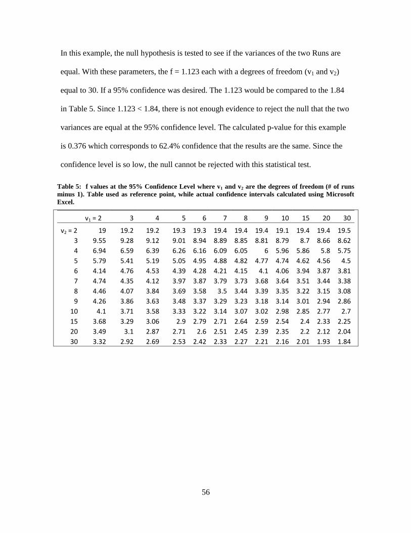
56

In this example, the null hypothesis is tested to see if the variances of the two Runs are

equal. With these parameters, the f = 1.123 each with a degrees of freedom (v1 and v2)

equal to 30. If a 95% confidence was desired. The 1.123 would be compared to the 1.84

in Table 5. Since 1.123 < 1.84, there is not enough evidence to reject the null that the two

variances are equal at the 95% confidence level. The calculated p-value for this example

is 0.376 which corresponds to 62.4% confidence that the results are the same. Since the

confidence level is so low, the null cannot be rejected with this statistical test.

Table 5: f values at the 95% Confidence Level where v1 and v2 are the degrees of freedom (# of runs

minus 1). Table used as reference point, while actual confidence intervals calculated using Microsoft

Excel.

v1 = 2 3 4 5 6 7 8 9 10 15 20 30

v2 = 2 19 19.2 19.2 19.3 19.3 19.4 19.4 19.4 19.1 19.4 19.4 19.5

3 9.55 9.28 9.12 9.01 8.94 8.89 8.85 8.81 8.79 8.7 8.66 8.62

4 6.94 6.59 6.39 6.26 6.16 6.09 6.05 6 5.96 5.86 5.8 5.75

5 5.79 5.41 5.19 5.05 4.95 4.88 4.82 4.77 4.74 4.62 4.56 4.5

6 4.14 4.76 4.53 4.39 4.28 4.21 4.15 4.1 4.06 3.94 3.87 3.81

7 4.74 4.35 4.12 3.97 3.87 3.79 3.73 3.68 3.64 3.51 3.44 3.38

8 4.46 4.07 3.84 3.69 3.58 3.5 3.44 3.39 3.35 3.22 3.15 3.08

9 4.26 3.86 3.63 3.48 3.37 3.29 3.23 3.18 3.14 3.01 2.94 2.86

10 4.1 3.71 3.58 3.33 3.22 3.14 3.07 3.02 2.98 2.85 2.77 2.7

15 3.68 3.29 3.06 2.9 2.79 2.71 2.64 2.59 2.54 2.4 2.33 2.25

20 3.49 3.1 2.87 2.71 2.6 2.51 2.45 2.39 2.35 2.2 2.12 2.04

30 3.32 2.92 2.69 2.53 2.42 2.33 2.27 2.21 2.16 2.01 1.93 1.84

57

IV. Analysis and Results

This chapter is intended to describe the analysis performed on the data

collected as described in chapter 3. Since the basis of the analysis revolves around the

curve fitting routines, the data fitting will be discussed in section 4.1. Afterwards, the

statistical analysis described in the chapter 3 will be performed on 4 different aspects of

the data acquired. This will lead to the conclusions drawn in chapter 5.

4.1 Data Fitting

After the each run finished, the raw data was saved to a text file and loaded in

MATLAB. The data in the file was restructured into an array for analysis. In order to

extract useful information from the raw data, the data needed to be fit to a model using

code in MATLAB called ‘peakfit.m’. The model required is non-linear and would not

work well with linear least squares curve fitting method that is considered simple and

fast. Instead the set of data was fit using the iterative method, which is a general fitting

routine that uses trial and error. The parameters are adjusted systematically until the

equation for the model chosen fits the data. There are 4 main steps that the code uses to

fit a model to the data [O’Haver]. First, a model for the data is selected. Second, an initial

guess for the non-linear parameters are chosen. Third, the ‘peakfit.m’ code computes the

model and compares it to the data set, calculating a fitting error. Lastly, if the fitting error

is greater than the required fitting accuracy, the code systematically changes one or more

of the parameters and loops back to step 3. The method that the code uses is the Nelder-

58

Mead method, which is a standard non-linear optimization technique that uses an

educated guess search method that can converge on non-stationary points.

As discussed previously, Mössbauer spectra are best fit with a Voigt function. If

the wrong model was chose, then the results would not be expected to be accurate. For

instance, a Lorentzian and a Gaussian model was fit to the same data that the Voigt was

fit. The Voigt model also has a peak shape parameter called ‘extra,’ which is a ratio of

the Lorentzian width to the Doppler width. Run19 and Run44I data were used as the

confirming the Voigt over the Lorentzian and the Gaussian. This can be seen in Figure

25. Both the short and long runs (Runs 19 and 44I respectively) had a lower fitting error

for the Voigt compared to the Gaussian and the Lorentzian. The larger the fitting errors

the larger the parameter errors, but the parameter errors are not equal to the fitting error.

Parameter errors are not given because the true peak values are not known before the

experiments were run. Also notice the residual plots for Run44I, the Voigt residuals are

much more random compared to the Gaussian and Lorentizian. Artifacts near the peaks

can be seen in the other two models. Due to the short acquisition time for Run19, artifacts

in the residuals near the peaks have not developed and appear random for all three.

For the type-310 stainless steel absorber, only one peak is identified in theory and

one peak was used for the analysis. During the analysis, an asymmetry was observed as

the peaks developed. We considered fitting two peaks to the data. The fitting error

decreased as expected, but the second peak was unstable in position, width, and height.

The second peak instability was observed in the in-experiment runs where the data was

saved multiple times to watch the peaks develop. This instability was due to the code

fitting to random noise and not an actual peak. Therefore, another method was used to

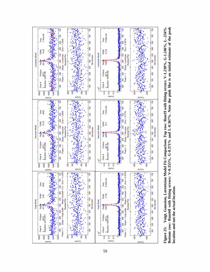
59

Fig

ure

25

:

Vo

igt,

Ga

uss

ian

, L

ore

ntz

ian

Mod

el F

it C

om

pari

son

. T

op

row

: R

un

19 w

ith

fit

tin

g e

rro

rs:

V-1

.23

8%

, G

-1.2

46

%,

L-.

23

4%

.

Bott

om

row

: R

un

44

I w

ith

fit

tin

g e

rrors

: V

-0.3

55%

, G

-0.3

71%

an

d L

-0.3

67%

. N

ote

th

e p

ink

lik

e is

an

in

itia

l es

tim

ate

of

the

pea

k

loca

tion

an

d n

ot

the

act

ual

loca

tio

n.

60

analyze the peak asymmetry and is discussed in section 4.2.3. This method makes better

use of the codes ability to fit a peak with noise and will be discussed next.

The fitting error that is calculated by the ‘peakfit.m’ code is a root-mean-square

difference between the model and the data. This error is minimized through the iterative

process discussed previously. The parameter errors are directly proportional to the noise

in the data and to the fitting error. Figure 26, taken from Thomas O’Haver, shows the

variability of the fitting error, which is caused by random small variations in the initial

guesses rather than the noise in the signal. Notice in the figure that the errors are the

smaller for peak position and worse for the peak height and width. The fitting error, as

well as the parameter errors, is dependent of the number of data points in the width of the

peak. The more points the code has to draw from the more accurate the fit. When the

experiment switched from 11mm/s to 22mm/s, the number of points to fit decreased. This

is because the number of energy bins (channels) that were utilized decreased and the

number of channels for the background increase due to the increase in motor velocity.

The data was run for a longer period of time to compensate for the fewer data points in

the narrower peak by increasing the signal to noise ratio.

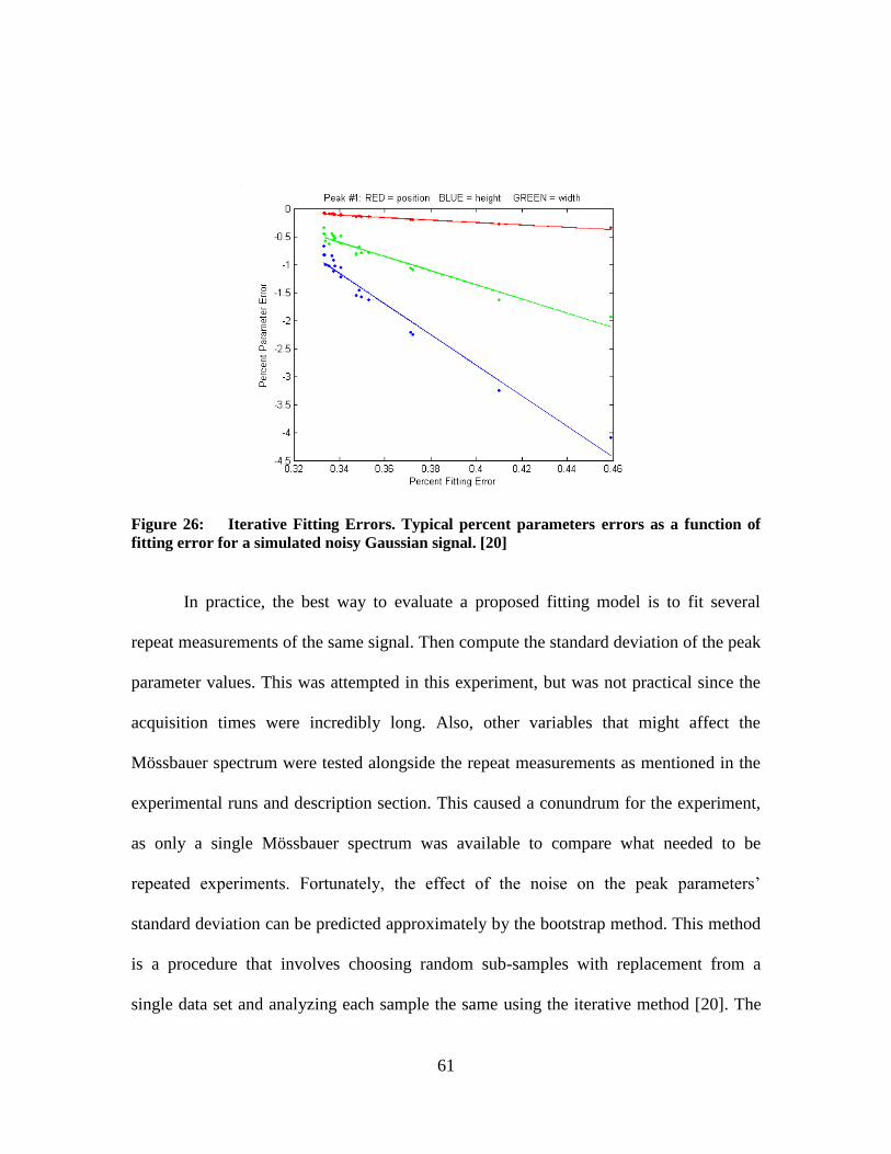
61

Figure 26: Iterative Fitting Errors. Typical percent parameters errors as a function of

fitting error for a simulated noisy Gaussian signal. [20]

In practice, the best way to evaluate a proposed fitting model is to fit several

repeat measurements of the same signal. Then compute the standard deviation of the peak

parameter values. This was attempted in this experiment, but was not practical since the

acquisition times were incredibly long. Also, other variables that might affect the

Mössbauer spectrum were tested alongside the repeat measurements as mentioned in the

experimental runs and description section. This caused a conundrum for the experiment,

as only a single Mössbauer spectrum was available to compare what needed to be

repeated experiments. Fortunately, the effect of the noise on the peak parameters’

standard deviation can be predicted approximately by the bootstrap method. This method

is a procedure that involves choosing random sub-samples with replacement from a

single data set and analyzing each sample the same using the iterative method [20]. The

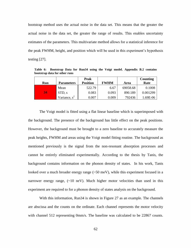
62

bootstrap method uses the actual noise in the data set. This means that the greater the

actual noise in the data set, the greater the range of results. This enables uncertainty

estimates of the parameters. This multivariate method allows for a statistical inference for

the peak FWHM, height, and position which will be used in this experiment’s hypothesis

testing [27].

Table 6: Bootstrap Data for Run34 using the Voigt model. Appendix B.2 contains

bootstrap data for other runs

Run Parameters

Peak

Position FWHM Area

Counting

Rate

34

Mean 522.79 6.67 69058.68 0.1008

STD, s 0.083 0.093 890.189 0.001299

Variance, s2 0.007 0.009 792436 1.69E-06

The Voigt model is fitted using a flat linear baseline which is superimposed with

the background. The presence of the background has little effect on the peak positions.

However, the background must be brought to a zero baseline to accurately measure the

peak heights, FWHM and areas using the Voigt model fitting routine. The background as

mentioned previously is the signal from the non-resonant absorption processes and

cannot be entirely eliminated experimentally. According to the thesis by Tanis, the

background contains information on the phonon density of states. In his work, Tanis

looked over a much broader energy range (~50 meV), while this experiment focused in a

narrower energy range, (~10 neV). Much higher motor velocities than used in this

experiment are required to for a phonon density of states analysis on the background.

With this information, Run34 is shown in Figure 27 as an example. The channels

are abscissa and the counts on the ordinate. Each channel represents the motor velocity

with channel 512 representing 0mm/s. The baseline was calculated to be 22867 counts.

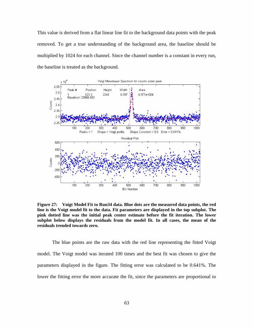
63

This value is derived from a flat linear line fit to the background data points with the peak

removed. To get a true understanding of the background area, the baseline should be

multiplied by 1024 for each channel. Since the channel number is a constant in every run,

the baseline is treated as the background.

Figure 27: Voigt Model Fit to Run34 data. Blue dots are the measured data points, the red

line is the Voigt model fit to the data. Fit parameters are displayed in the top subplot. The

pink dotted line was the initial peak center estimate before the fit iteration. The lower

subplot below displays the residuals from the model fit. In all cases, the mean of the

residuals trended towards zero.

The blue points are the raw data with the red line representing the fitted Voigt

model. The Voigt model was iterated 100 times and the best fit was chosen to give the

parameters displayed in the figure. The fitting error was calculated to be 0.641%. The

lower the fitting error the more accurate the fit, since the parameters are proportional to

64

the fitting error. The subplot represents the residuals left over from the fit. The residuals

should be uniform and random, where-as not to produce artifacts near the fitted peak. The

mean of the residuals is 6.1E-13, essentially zero (as is the case with all runs where the

residual means were calculated). This indicates a good and unbiased fit. The peak

parameters were measured using the bootstrap method with N =100, where N is the

number of trials for each bootstrap iteration and can be seen in Table 6. The sample

standard deviation, s, is given for each parameter. The sample variance is: s2. Since the

bootstrap method randomly samples the data, greater noise will lead to greater variability

in the parameters.

4.2 Statistical Analysis

There are three parameters that the following statistical analyses focus on:

FWHM, peak counting rate and background counting rate. The FWHM is pulled directly

from the peak fitting routine, while the peak counting rate and the background counting

rate are normalized by dividing the peak area and the baseline from the fitting routine by

the acquisition time. The counting rates were then corrected for the source decay shown

in Figure 13 by assuming the 57

Co source had a normalized activity of 1 on the date the

data acquisition started, 10 May 2012. The normalized activity for the last run was 0.467.

To correct for source decay, each counting rate was divided by the normalized activity.

This allows for an equitable comparison of counting rates between experiments. There

are, however, various variable changes from Run set to Run set shown in Table 4.

One example to note is the motor velocity changing from 11mm/s to 22mm/s.

This increases the energy range of the incident 14.4 keV gamma, which means that there

65

is a narrower channel band allocated to the resonant absorptions. This decreases the

FWHM, but keeps the peak height the same; therefore, decreasing the area under the

peak. This might sound counter intuitive, but less time is spent in resonance (the motor

sweeps faster) and gammas from the Mössbauer source have less of a chance to arrive at

the absorber with the correct energy. The same effect is seen in the background baseline,

which decreases the background counting rate of the 22mm/s compared to the 11mm/s

run. Because of these reasons, the 11mm/s data cannot be compared to the 22mm/s data

and have to be treated separately. One parameter that does not change is the peak

location. But due to the age of the motor, the equipment did not remain in perfect

calibration which caused slight shifts the peak locations. Occasional recalibration of the

motor was required. Since the calibration of the motor required visually minimizing the

interface pattern from Michelson interferometer in the laser diode of the motor, there

were slight adjustments in the peak location. Fortunately, this does not affect the

statistical analyses since peak location was not taken into consideration and the peak

location did not affect the shape of the Mössbauer spectrum peak. The peak did slightly

oscillate during the runs, but did not continuously drift in a preferential direction, which

would have skewed the results of the peak asymmetry analysis. The level and period of

the oscillation would need to be investigated further.

4.2.1 Experimental Run Analysis

The ideal statistical analysis would compare many spectra with a phonon source

to many spectra without a phonon source. While all other variables like absorber material

length, motor velocity, phonon source, detector gain, and detector gas would remain

66

constant. Unfortunately, due to the time limit and refinement of the experimental process

as time progressed, some of these variables did change. Fortunately, at least one spectrum

with a phonon source and no phonon source were taken before a variable change. Due to

limited sample sizes, the resulting statistics would be very poor if one just compared one

spectrum to another. A percent difference would not give any insight to whether or not

the null hypothesis can be rejected. To add meaning to a spectrum to spectrum

comparison, the bootstrap method mentioned previously was implemented. In essence,

the method produces a hundred independent trial runs for each spectrum by replacing a

percentage of the data points randomly with other random data points in the spectrum.

There is substantial evidence that this method can be effectively used to give a standard

deviation of the FWHM and peak counting rate parameter [20, 27]. All the bootstrap data

can be seen summarized in Appendix B.2. The background was not included in the

bootstrap data. To get an overall perspective of the data (given in Appendix B.1)

variability, comparisons were made as a whole shown in Figure 28, Figure 29, and Figure

30.

The first comparison, Figure 28, was to see the how the peak and background

compared to each other for the 11mm/s motor velocity. As shown in the figure, the

counting rate for both the peak and background counts decreased over time even with the

Mössbauer source decay correction. Also, both the phonon source and no source run

groupings held the same trend. The runs with a phonon source showed more variability in

the peak counting rate, while the opposite was true for the source run background

counting rate. Note it was observed that the detector bias shut off at some point between

Runs 25A & B and 26B & C. Since the bias shut off for these, Runs 25B-E and 26C were

67

excluded from the statistical comparison. For the counting rate comparisons, there is a

70% confidence that the null result can be rejected for the peak and a 57% confidence to

reject the null result for the background. Statistically, the null result cannot be rejected

from this test.

The next comparison is for the 22mm/s motor velocity regime and can be found in

Figure 29. For row (a), the counting rates are uniform barring the Run39 outlier. The

most likely reason Run39 was off is the electronics. The motor was velocity was changed

to 22mm/s and recalibrated from Run38. After Run39, the motor started acting up and

had to be fixed and recalibrated for Run40. To make sure the motor remained in working

order for each run afterwards; it was recalibrated and monitored after each run.

Unfortunately, this did not help the data acquisition for Runs 42G, 43A, and 45B-C.

The detector bias tripped for those runs, which would explain the large

oscillations in those runs. These runs and Run39 were not included in the statistical

analysis shown in Table 7. The F test was applied with these exclusions and for the peak

counting rate there is a 92.3% confidence that the null result can be rejected. For the

background counting rate there is an 87.6% confidence that the null result can be

rejected. Unfortunately, more test should be ran for the data to have more confidence in

the test performed. The runs with no source and a source were one long data run for each

and saved at various intervals. Technically, there were 2 runs without a source and 3 runs

with a source. The evolution of each run was analyzed in the next section.

The last comparison made on the data as a whole was between the FWHM with

and without the phonon source for the 11mm/s and 22mm/s motor velocity, shown in

Figure 30. For the FWHM statistical analysis, the same runs were excluded that were

68

excluded in the peak and background counting rate comparisons. In Table 7, the

confidences for the FWHM were calculated. For the 11mm/s motor velocity, there is only

a 12% confidence that the null result can be rejected. Curiously, for the 22mm/s motor

velocity, there is a 92.8% confidence that the null result can be rejected. The disparity

between the 11mm/s and the 22mm/s confidence levels sends a mixed message on

whether the null result can be accepted or rejected. A possible reason for the disparity is

the number of ‘independent’ runs for the 11mm/s compared to the 22mm/s. Further data

collection would be required to truly understand the disparity.

69

Ta

ble

7:

Sta

tist

ica

l co

mp

ari

son

s fo

r p

ho

no

n s

ou

rce a

nd

no

ph

on

on

so

urc

e i

n F

igu

re 2

8,

Fig

ure

29

, a

nd

Fig

ure

30

. T

he

f-te

st w

as

the

pri

ma

ry m

eth

od

use

d t

o c

alc

ula

te a

p-v

alu

e a

nd

a c

on

fid

ence

in

terv

al

for

the

FW

HM

, th

e

pea

k a

nd

ba

ck

gro

un

d c

ou

nti

ng

ra

tes.

No P

hon

on

Sou

rce

vs

Ph

on

on

Sou

rce

Mo

tor

Vel

oci

ty

Sta

tist

ic

Pea

k C

ou

nti

ng R

ate

B

ack

gro

un

d C

ou

nti

ng

Rate

FW

HM

No S

ou

rce

Sou

rce

No S

ou

rce

Sou

rce

No

So

urc

e S

ou

rce

11

mm

/s

Mea

n

0.1

185

0.1

237

58.3

6

59.1

5

7.2

85

7.5

76

s 0.0

185

0.0

130

7.0

9

5.4

3

0.7

58

0.8

13

Var

ian

ce, s2

0.0

003

0.0

002

50.3

1

29.4

6

0.5

75

0.6

61

F t

est

p-v

alue

0.3

003

0.4

271

0.8

79

3

Co

nfi

den

ce %

70

%

57.3

%

12

.1%

22

mm

/s

Mea

n

0.0

236

0.0

231

17.7

4

16.4

3

3.5

76

3.8

04

s 0.0

012

0.0

020

2.2

0

3.4

2

0.1

21

0.0

69

5

Var

ian

ce, s2

1.5

1E

-6

4.1

7E

-6

4.5

6

11.7

0

0.0

15

0.0

05

F t

est

p-v

alue

0.0

770

0.1

242

0.0

717

Co

nfi

den

ce %

92.3

%

87.6

%

92

.8%

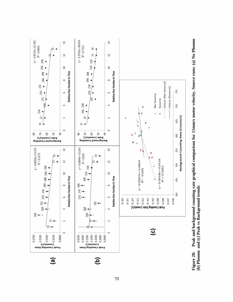
70

Fig

ure

28

:

Pea

k a

nd

back

gro

un

d c

ou

nti

ng r

ate

gra

ph

ical

com

pari

son

for

11m

m/s

moto

r v

elo

city

. S

ou

rce

run

s: (

a)

No

Ph

on

on

(b)

Ph

on

on

a

nd

(c)

Pea

k v

s B

ack

gro

un

d t

ren

ds

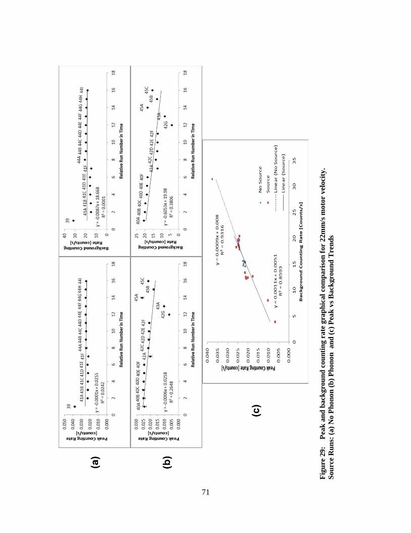
71

Fig

ure

29

: P

eak

an

d b

ack

gro

un

d c

ou

nti

ng r

ate

gra

ph

ical

com

pari

son

for

22m

m/s

moto

r vel

oci

ty.

Sou

rce

Ru

ns:

(a

) N

o P

ho

no

n (

b)

Ph

on

on

an

d (

c) P

eak

vs

Back

gro

un

d T

ren

ds

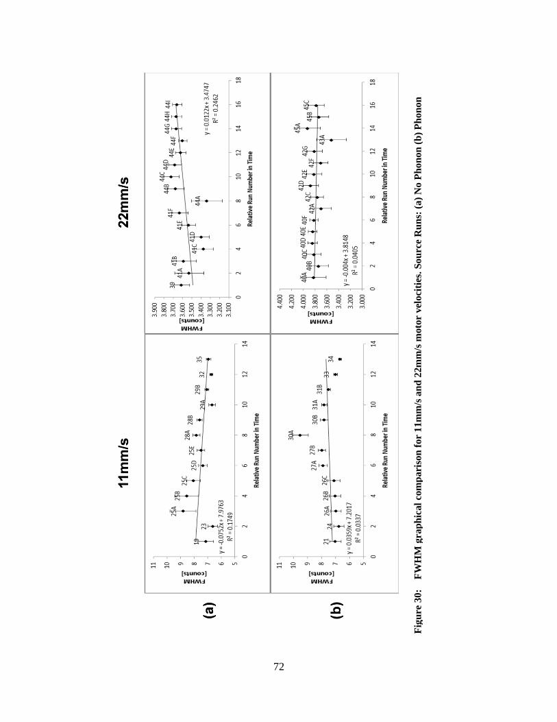
72

Fig

ure

30

: F

WH

M g

rap

hic

al

com

pari

son

for

11m

m/s

an

d 2

2m

m/s

moto

r vel

oci

ties

. S

ou

rce

Ru

ns:

(a

) N

o P

ho

no

n (

b)

Ph

on

on

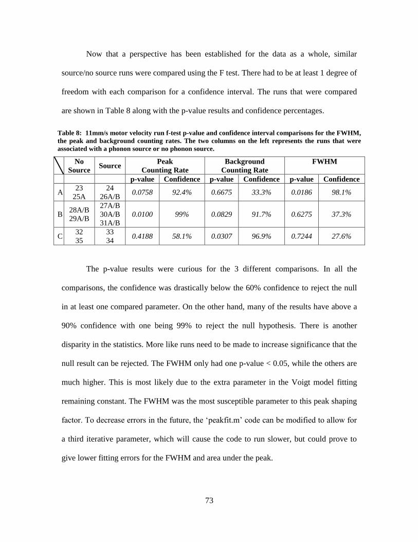
73

Now that a perspective has been established for the data as a whole, similar

source/no source runs were compared using the F test. There had to be at least 1 degree of

freedom with each comparison for a confidence interval. The runs that were compared

are shown in Table 8 along with the p-value results and confidence percentages.

Table 8: 11mm/s motor velocity run f-test p-value and confidence interval comparisons for the FWHM,

the peak and background counting rates. The two columns on the left represents the runs that were

associated with a phonon source or no phonon source.

No

Source Source

Peak

Counting Rate

Background

Counting Rate

FWHM

p-value Confidence p-value Confidence p-value Confidence

A 23

25A

24

26A/B 0.0758 92.4% 0.6675 33.3% 0.0186 98.1%

B 28A/B

29A/B

27A/B

30A/B

31A/B

0.0100 99% 0.0829 91.7% 0.6275 37.3%

C 32

35

33

34 0.4188 58.1% 0.0307 96.9% 0.7244 27.6%

The p-value results were curious for the 3 different comparisons. In all the

comparisons, the confidence was drastically below the 60% confidence to reject the null

in at least one compared parameter. On the other hand, many of the results have above a

90% confidence with one being 99% to reject the null hypothesis. There is another

disparity in the statistics. More like runs need to be made to increase significance that the

null result can be rejected. The FWHM only had one p-value < 0.05, while the others are

much higher. This is most likely due to the extra parameter in the Voigt model fitting

remaining constant. The FWHM was the most susceptible parameter to this peak shaping

factor. To decrease errors in the future, the ‘peakfit.m’ code can be modified to allow for

a third iterative parameter, which will cause the code to run slower, but could prove to

give lower fitting errors for the FWHM and area under the peak.

74

4.2.2 In-experiment Development and Variances

Even though it may look like there are 30 different experiments for Runs 40A-F,

41A-F, 42A-G, 44A-I, and Run 45A-C, they are technically only 5 long running

experiments with the data saved periodically during the run. Because of this, the

development of the signal can be studied, allowing a check to see if the peak

development proceeds as expected by comparing the standard deviations and variances.

Figure 31 gives a visual representation on the peak development. All the bootstrap fitting

routine results can be seen in Appendix B.2. All the Voigt fitting data can be seen in

Appendix B.1. All peak locations remained stable within the individual runs (ex. 40A-F),

as expected, but slightly shifted (max shift 1.34 channels) between these run sets. Runs

42G and 45A-C will be excluded due to the voltage bias shutting off during the run. What

will be looked at in this section will be the normalized peak height, peak counting rate

and FWHM. The normalized peak height was determined by dividing the height by the

hourly counting rate. The value would describe how the peak height grows per hour.

Table 9: In-experiment peak development statistics for the 22mm/s motor velocity

runs. Parameters: mean, standard deviation (STD) and variance of each all the

runs in a set. Example: Run set 40, runs in the set A-F.

Parameter Normalized

Peak Height

FWHM

Peak Counting

Rate

Run 40A-F

Mean 7.169 3.813 0.0246

STD 0.110 0.035 0.000254

Variance 0.0122 0.0012 6.47E-08

Run 41A-F

Mean 7.047 3.507 0.0222

STD 0.231 0.095 0.000342

Variance 0.0532 0.0090 1.17E-07

Run 42A-F

Mean 6.121 3.769 0.0209

STD 0.104 0.068 0.000475

Variance 0.0109 0.0047 2.25E-07

Run 44A-I

Mean 7.591 3.623 0.0246

STD 0.227 0.107 0.000194

Variance 0.0513 0.0114 3.76E-08

75

Figure 31: Peak Development for In-Experiment Runs. Peaks are the Voigt fit to the data.

Top: Run40A-F. Bottom: Run44A-I.

As the peaks developed, the fitting error decreased along with the variances on the

normalized peak height, the peak counting rate and the FWHM. This is as expected due

to the stabilization of the peak with an increased counting time. The number of counts

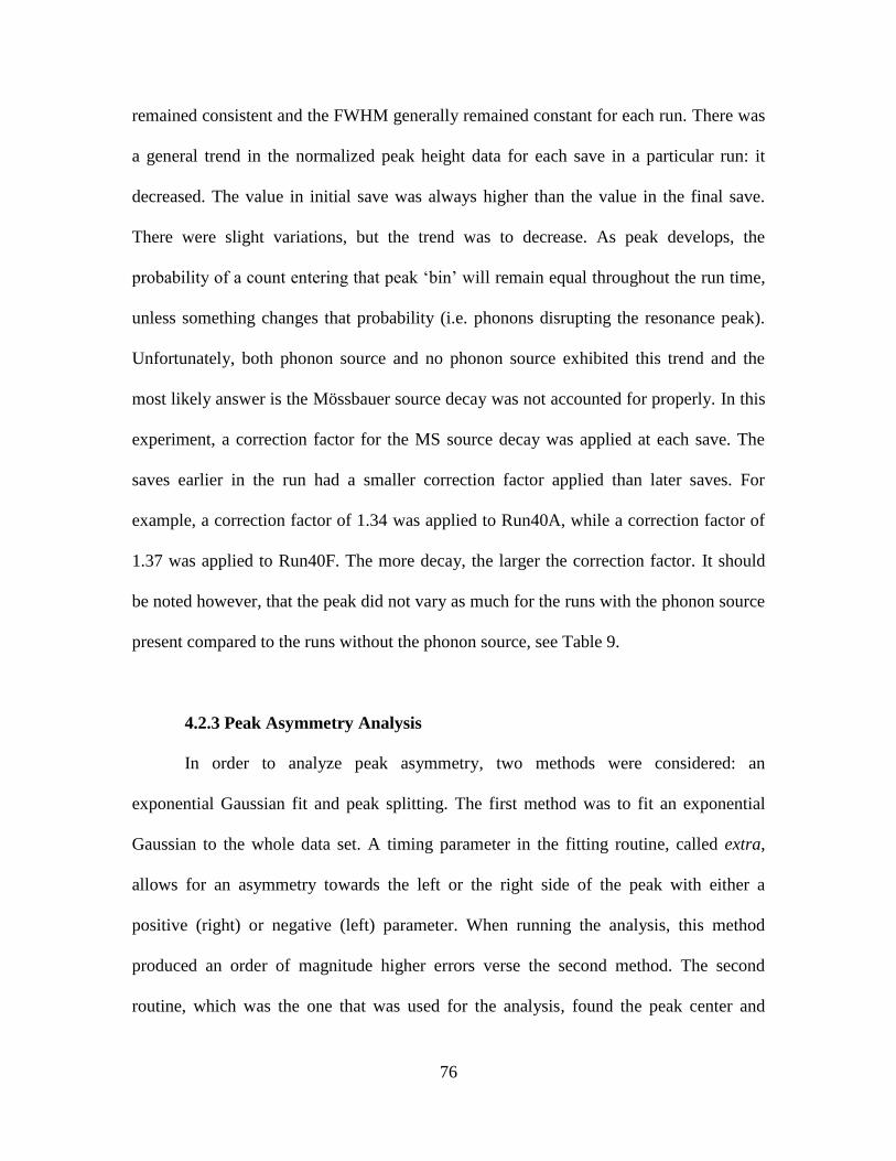
76

remained consistent and the FWHM generally remained constant for each run. There was

a general trend in the normalized peak height data for each save in a particular run: it

decreased. The value in initial save was always higher than the value in the final save.

There were slight variations, but the trend was to decrease. As peak develops, the

probability of a count entering that peak ‘bin’ will remain equal throughout the run time,

unless something changes that probability (i.e. phonons disrupting the resonance peak).

Unfortunately, both phonon source and no phonon source exhibited this trend and the

most likely answer is the Mössbauer source decay was not accounted for properly. In this

experiment, a correction factor for the MS source decay was applied at each save. The

saves earlier in the run had a smaller correction factor applied than later saves. For

example, a correction factor of 1.34 was applied to Run40A, while a correction factor of

1.37 was applied to Run40F. The more decay, the larger the correction factor. It should

be noted however, that the peak did not vary as much for the runs with the phonon source

present compared to the runs without the phonon source, see Table 9.

4.2.3 Peak Asymmetry Analysis

In order to analyze peak asymmetry, two methods were considered: an

exponential Gaussian fit and peak splitting. The first method was to fit an exponential

Gaussian to the whole data set. A timing parameter in the fitting routine, called extra,

allows for an asymmetry towards the left or the right side of the peak with either a

positive (right) or negative (left) parameter. When running the analysis, this method

produced an order of magnitude higher errors verse the second method. The second

routine, which was the one that was used for the analysis, found the peak center and

77

compared the left and right side of the peak. This was accomplished by splitting the data

at the peak center where the left and right data points were mirrored with themselves to

produce two new symmetric spectra to analyze. One spectra was the left mirrored and the

other was the right mirrored. The spectra were fitted with the Voigt fitting routine

described in the previous section. The MATLAB code for this process can be seen in

Appendix A.2. The two spectra were compared and the differences were compared with

each other as well as the other left and right spectra generated from the other runs.

There characteristics of the spectra were compared: the peak area counting rate,

the background counting rate, and the FWHM. Data can be seen in Appendix B.3. An F

test was done on all the spectra characteristics. It was discussed to use a t-test for an

additional analysis, but the parameters being tested were the mean of the distributions.

To be significantly different the probability (p-value) of the test need to be <0.05 to have

a 95% confidence that the null result can be rejected, anything >0.10 the null result

cannot be rejected. Before the left and right side of the peaks were compared, the left side

runs with a source were compared to the runs without a source for the 11mm/s and the

22mm/s data sets. Then same was done for the right side peaks. This was to give another

check to see if differences in the spectra are statistically significant. After this, the left

side runs without a source were compared to the right side runs with a source. The data

runs that were compared and analyzed can be seen in Table 6.

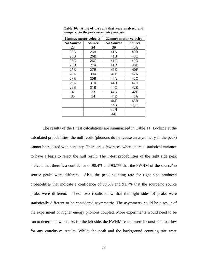
78

Table 10: A list of the runs that were analyzed and

compared in the peak asymmetry analysis

11mm/s motor velocity 22mm/s motor velocity

No Source Source No Source Source

23 24 39 40A

25A 26A 41A 40B

25B 26B 41B 40C

25C 26C 41C 40D

25D 27A 41D 40E

25E 27B 41E 40F

28A 30A 41F 42A

28B 30B 44A 42C

29A 31A 44B 42D

29B 31B 44C 42E

32 33 44D 42F

35 34 44E 45A

44F 45B

44G 45C

44H

44I

The results of the F test calculations are summarized in Table 11. Looking at the

calculated probabilities, the null result (phonons do not cause an asymmetry in the peak)

cannot be rejected with certainty. There are a few cases where there is statistical variance

to have a basis to reject the null result. The F-test probabilities of the right side peak

indicate that there is a confidence of 90.4% and 93.7% that the FWHM of the source/no

source peaks were different. Also, the peak counting rate for right side produced

probabilities that indicate a confidence of 88.6% and 91.7% that the source/no source

peaks were different. These two results show that the right sides of peaks were

statistically different to be considered asymmetric. The asymmetry could be a result of

the experiment or higher energy phonons coupled. More experiments would need to be

run to determine which. As for the left side, the FWHM results were inconsistent to allow

for any conclusive results. While, the peak and the background counting rate were

79

consistent with low confidence levels. To use the 11mm/s velocity regime, the p-values

would show a trend a trend that the peak counting rate remained the same and the FWHM

could be different. A different conclusion would be drawn if the 22mm/s were only

considered. The 22mm/s regime would indicate that the right sides of the peaks were

different when considering the peak counting rate and the FWHM. At the same time there

is low confidence that there was a change in the left side of the peak. This could indicate

a peak asymmetry. The motor velocity would not have such an effect on the results, since

it does not change the environment of the absorber. More data collection would be

required.

Table 11: Calculated f-test p-values and confidence intervals for Peak Asymmetry. Top: Comparison of

phonon source and no source for the left and right side of the peaks. Bottom: Comparison of the left and

right side of the peaks for a phonon source and no source. For each comparison, the 11mm/s and 22mm/s

motor velocity runs should not be compared with each other.

Motor Velocity No Source vs Source

Left Side Right Side

Peak

Counting

Rate

Bkgd

Counting

Rate

FWHM Peak

Counting

Rate

Bkgd

Counting

Rate

FWHM

11mm/s p-value 0.852 0.667 0.165 0.114 0.684 0.096

Confidence 14.8% 33.3% 83.5% 88.6% 31.6% 90.4%

22mm/s p-value 0.372 0.469 0.750 0.083 0.473 0.063

Confidence 62.8% 53.1% 25.0% 91.7% 52.7% 93.7%

Left Side Peak verse Right Side peak

Motor Velocity Peak Counting Rate Background Counting

Rate

FWHM

No Source Source No Source Source No Source Source

11mm/s p-value 0.25 0.52 0.999 0.993 0.0041 0.96

Confidence 75.0% 48.0% 0.1% 0.7% 99.6% 4.0%

22mm/s p-value 0.20 0.73 0.997 0.998 0.918 0.165

Confidence 80.0% 27.0% 0.3% 0.2% 8.2% 83.5%

Another analysis was done to compare the left side and right side of the peak for

both the source and no source runs. Our statistical analysis of the data produced a curious

80

result similar to the source/no source analysis of the left side of the peak. A high p-value

for the F test would indicate no difference between two samples, while a low p-value

would indicate a difference. We would expect that there would be no difference between

the left and right side of the peak when phonons are not present or there is a natural

phenomenon that causes an asymmetry in the peak. Additionally, when phonons are

present we would expect that they would create an asymmetry where there is not one or

vice versa. When analyzing the peak counting rate data for the left/right side peak

comparisons, there is no confidence to determine whether there is or is not a difference in

the peak, as shown in Table 11. For the FWHM, the 11mm/s motor velocity regime’s p-

values indicate the no source runs have a 99.6% confidence that the right and left side are

asymmetric and the source runs have a 96% confidence that the right and left side peaks

are symmetric. While the 22mm/s motor velocity produced p-values that were much less

confident and would produce opposite conclusions.

4.2.4 Heat Tape

As explained in Chapter 3, another phonon source was used to see if there would

be a better signal change. Heat tape was added to the bar in Runs 36, 37 and 38. The

temperatures ranged from room temperature to 35°C and then 46°C. As the spectra

developed, there did not seem to be differences in the peaks. The bootstrap method with

the variances and the peaks increase in the FWHM (6.35, 6.76, and 6.91, respectively)

would indicate that phonons would have an effect; especially since the standard deviation

di not overlap between Run38 and the other two runs. More data would need to be taken

to statistically confirm. Since time did not permit, a phone call was made to Dr.

81

Spikerman, the developer of the Mössbauer spectrometers Ranger Scientific Instruments,

to see what temperature the bar needed to be heated. He said that the bar would need to

be heated to about 1000°C to see a broadening in the peaks. This stopped the pursuit of

this path. The data and Voigt fits can be seen in the appendices.

82

V. Conclusions and Recommendations

5.1 Summary

The experiment developed was set up to investigate whether nuclear induced

phonons would have a visible effect on a Mössbauer spectrum. Stainless steel type-310

was used as the Mössbauer absorber material because it has three properties that would

allow the investigation to occur. The first property is the 57

Fe in the material that allows

for a resonant absorption with the 57

Co Mössbauer source. The second property is the

single peak spectrum produced by the Mössbauer events. This property simplified the

analysis to focus on the properties of a single peak and preclude any overlapping nature

of other peaks. Lastly, the stainless steel has a stiffness that would allow for acoustic

propagations and increased probability of a phonon coupling with a Mössbauer event. An

alpha source, 241

Am, was used to induce phonons through the nuclear recoil produced

from Rutherford scattering. To verify that that phonons induced by the alpha source had

an effect, Mössbauer spectra with and without a phonon source were compared. Other

experimental variables were to remain constant. Unfortunately, since the equipment was

old, a few modifications to experiment were necessary to keep the experiment running

and try to increase the likelihood that a phonon interaction with the Mössbauer events to

occur.

Since there was not an obvious change in the 62 spectra acquired, hypothesis

testing was used to see if there actually was a significant difference between the phonon

and no phonon spectra. The null hypothesis tested was that phonons did not couple with

the Mössbauer spectra. The statistical analysis used a two tailed F-distribution. This test

is most common when comparing functions models fit to a data set by using analysis of

83

variance. The comparisons that were looked at were changes in the a few parameters of

the Voigt peak fit the data: FWHM, peak counting rate, and background counting rate. A

shift in the peak centroid was not considered. The comparisons were done in the 11mm/s

and the 22mm/s motor velocity regime. The data was compared as a whole between

phonon source and no phonon source spectra. Then related runs were compared, as

shown in Table 8 for the 11mm/s regime. It was determined that was not enough

evidence to reject the null hypothesis for these tests. While some of the tests produced a

95% confidence interval, others produced less than 60% confidence. These results were

conflicting.

The same conflict between confidence intervals came about when peak

asymmetry was analyzed. In the analysis of the asymmetry, the peaks were mirrored

about the centroid and the left and right sides were compared as if they were two separate

symmetric Voigt peaks. The same parameters as before were compared, Table 11. The

statistics in comparing one motor regime to another were conflicting and more tests

would be required to confidently reject the null.

Another consideration to analyze was to check on how the peaks developed. This

was accomplished with the 22mm/s motor regime. Five long runs, about 2 weeks each,

were saved periodically. When the peak development was analyzed, the peaks developed

as expected. It was noted that the peaks with no phonon source appeared to fluctuate

more compared to the phonon source runs. It was not concluded that this is possible

evidence to reject the null, but that further testing would be required to have confidence

whether or not the null can be rejected. There is a possibility that changes in the side

84

wings were outside the energy window established in this thesis. And the motor velocity

should be increased and analyzed.

5.2 Significance of Research

As far as the author and his committee are aware, this research is the first to be

done in this area of study. The coupling of phonons with Mössbauer events using a

radiation source; in order, to detect the radiation source has not be attempted. The initial

results, which this thesis provides, cannot say with certainty either way whether the

phonon do substantially affect the Mössbauer spectra; there is indication either way to

reject the null. The experiment would need to be refined to determine if this method can

be used as a solid state detector for various radiation sources.

5.3 Future Work

There are a few methods that can be used to generate higher confidence whether

the null result can be rejected.

Cool the stainless steel bar to temperatures close to 77K using liquid nitrogen.

This would decrease the inherent oscillations of the atoms in the stainless

steel. It is predicted that this decrease in random vibrations would make any

changes to the resonant peak more sensitive to the nuclear induced radiation.

Create a solenoid to verify that induced phonons can couple with Mössbauer

events. Copper wire would be wrapped around the stainless steel absorber and

current would be passed through the wire to create the solenoid. Then the

electric current would be oscillated to create pole flipping in the stainless steel

85

that would induce phonons. The frequency of the oscillation would need to

high enough to allow for and increased probability coincident

phonon/Mössbauer events to occur. It would be best to perform simulations to

verify the frequency of the electric current oscillations.

Change the absorber and the phonon source used in the experiment. The

recommended changes in the absorber would be a magnetic material to help

directionalize the phonon propagation by aligning the grains and magnetic

poles. One material to use would be Neodymium (Nd2Fe14B). This material

contains a majority of iron for Mössbauer spectroscopy. Also, the material has

boron which would be perfect for neutrons to be used as the phonon source.

Natural boron contains 20% 10

B and 10

B is good thermal neutron absorber.

Another material would be boron carbide with an enriched 57

Fe surface. The

boron carbide is an extremely hard ceramic material that has a uniform

crystalline structure. The material would be ideal for phonon propagation,

since most of the literature recommends crystalline structures to reduce

dispersion in phonon propagation. The enrichment of one surface with 57

Fe

would increase the Mössbauer event counting rate and allow for a better signal

to noise ratio.

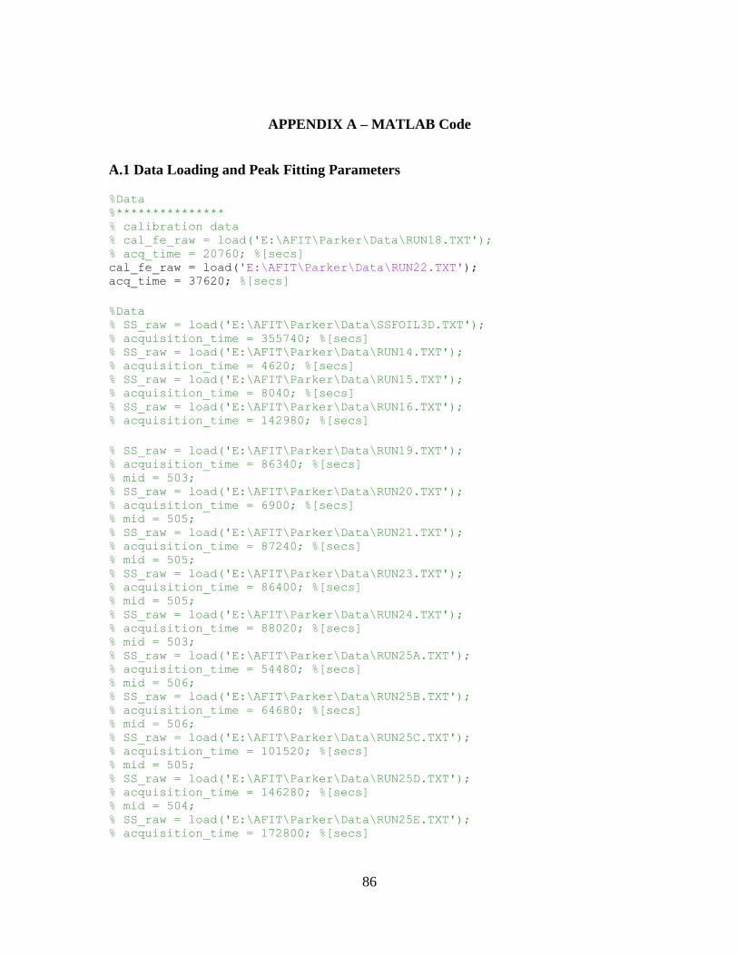
86

APPENDIX A – MATLAB Code

A.1 Data Loading and Peak Fitting Parameters

%Data %*************** % calibration data % cal_fe_raw = load('E:\AFIT\Parker\Data\RUN18.TXT'); % acq_time = 20760; %[secs] cal_fe_raw = load('E:\AFIT\Parker\Data\RUN22.TXT'); acq_time = 37620; %[secs]

%Data % SS_raw = load('E:\AFIT\Parker\Data\SSFOIL3D.TXT'); % acquisition_time = 355740; %[secs] % SS_raw = load('E:\AFIT\Parker\Data\RUN14.TXT'); % acquisition_time = 4620; %[secs] % SS_raw = load('E:\AFIT\Parker\Data\RUN15.TXT'); % acquisition_time = 8040; %[secs] % SS_raw = load('E:\AFIT\Parker\Data\RUN16.TXT'); % acquisition_time = 142980; %[secs]

% SS_raw = load('E:\AFIT\Parker\Data\RUN19.TXT'); % acquisition_time = 86340; %[secs] % mid = 503; % SS_raw = load('E:\AFIT\Parker\Data\RUN20.TXT'); % acquisition_time = 6900; %[secs] % mid = 505; % SS_raw = load('E:\AFIT\Parker\Data\RUN21.TXT'); % acquisition_time = 87240; %[secs] % mid = 505; % SS_raw = load('E:\AFIT\Parker\Data\RUN23.TXT'); % acquisition_time = 86400; %[secs] % mid = 505; % SS_raw = load('E:\AFIT\Parker\Data\RUN24.TXT'); % acquisition_time = 88020; %[secs] % mid = 503; % SS_raw = load('E:\AFIT\Parker\Data\RUN25A.TXT'); % acquisition_time = 54480; %[secs] % mid = 506; % SS_raw = load('E:\AFIT\Parker\Data\RUN25B.TXT'); % acquisition_time = 64680; %[secs] % mid = 506; % SS_raw = load('E:\AFIT\Parker\Data\RUN25C.TXT'); % acquisition_time = 101520; %[secs] % mid = 505; % SS_raw = load('E:\AFIT\Parker\Data\RUN25D.TXT'); % acquisition_time = 146280; %[secs] % mid = 504; % SS_raw = load('E:\AFIT\Parker\Data\RUN25E.TXT'); % acquisition_time = 172800; %[secs]

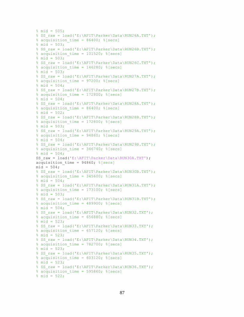
87

% mid = 505; % SS_raw = load('E:\AFIT\Parker\Data\RUN26A.TXT'); % acquisition_time = 86400; %[secs] % mid = 503; % SS_raw = load('E:\AFIT\Parker\Data\RUN26B.TXT'); % acquisition_time = 101520; %[secs] % mid = 503; % SS_raw = load('E:\AFIT\Parker\Data\RUN26C.TXT'); % acquisition_time = 146280; %[secs] % mid = 503; % SS_raw = load('E:\AFIT\Parker\Data\RUN27A.TXT'); % acquisition_time = 97200; %[secs] % mid = 504; % SS_raw = load('E:\AFIT\Parker\Data\RUN27B.TXT'); % acquisition_time = 172800; %[secs] % mid = 504; % SS_raw = load('E:\AFIT\Parker\Data\RUN28A.TXT'); % acquisition_time = 86400; %[secs] % mid = 502; % SS_raw = load('E:\AFIT\Parker\Data\RUN28B.TXT'); % acquisition_time = 172800; %[secs] % mid = 503; % SS_raw = load('E:\AFIT\Parker\Data\RUN29A.TXT'); % acquisition_time = 94860; %[secs] % mid = 504; % SS_raw = load('E:\AFIT\Parker\Data\RUN29B.TXT'); % acquisition_time = 346740; %[secs] % mid = 504; SS_raw = load('E:\AFIT\Parker\Data\RUN30A.TXT'); acquisition_time = 94860; %[secs] mid = 504; % SS_raw = load('E:\AFIT\Parker\Data\RUN30B.TXT'); % acquisition_time = 345600; %[secs] % mid = 504; % SS_raw = load('E:\AFIT\Parker\Data\RUN31A.TXT'); % acquisition_time = 173100; %[secs] % mid = 503; % SS_raw = load('E:\AFIT\Parker\Data\RUN31B.TXT'); % acquisition_time = 489900; %[secs] % mid = 504; % SS_raw = load('E:\AFIT\Parker\Data\RUN32.TXT'); % acquisition_time = 656880; %[secs] % mid = 523; % SS_raw = load('E:\AFIT\Parker\Data\RUN33.TXT'); % acquisition_time = 657120; %[secs] % mid = 523; % SS_raw = load('E:\AFIT\Parker\Data\RUN34.TXT'); % acquisition_time = 782700; %[secs] % mid = 523; % SS_raw = load('E:\AFIT\Parker\Data\RUN35.TXT'); % acquisition_time = 603120; %[secs] % mid = 523; % SS_raw = load('E:\AFIT\Parker\Data\RUN36.TXT'); % acquisition_time = 595860; %[secs] % mid = 522;

88

% SS_raw = load('E:\AFIT\Parker\Data\RUN37.TXT'); % acquisition_time = 601800; %[secs] % mid = 522; % SS_raw = load('E:\AFIT\Parker\Data\RUN38.TXT'); % acquisition_time = 327900; %[secs] % mid = 523; % SS_raw = load('E:\AFIT\Parker\Data\RUN39.TXT'); % acquisition_time = 591000; %[secs] % mid = 508; % SS_raw = load('E:\AFIT\Parker\Data\RUN40A.TXT'); % acquisition_time = 439800; %[secs] % mid = 508; % SS_raw = load('E:\AFIT\Parker\Data\RUN40B.TXT'); % acquisition_time = 862500; %[secs] % mid = 509; % SS_raw = load('E:\AFIT\Parker\Data\RUN40C.TXT'); % acquisition_time = 1056000; %[secs] % mid = 509; % SS_raw = load('E:\AFIT\Parker\Data\RUN40D.TXT'); % acquisition_time = 1479000; %[secs] % mid = 509; % SS_raw = load('E:\AFIT\Parker\Data\RUN40E.TXT'); % acquisition_time = 1560900; %[secs] % mid = 509; % SS_raw = load('E:\AFIT\Parker\Data\RUN40F.TXT'); % acquisition_time = 1839300; %[secs] % mid = 509; % SS_raw = load('E:\AFIT\Parker\Data\RUN41A.TXT'); % acquisition_time = 419700; %[secs] % mid = 509; % SS_raw = load('E:\AFIT\Parker\Data\RUN41B.TXT'); % acquisition_time = 603000; %[secs] % mid = 509; % SS_raw = load('E:\AFIT\Parker\Data\RUN41C.TXT'); % acquisition_time = 855000; %[secs] % mid = 509; % SS_raw = load('E:\AFIT\Parker\Data\RUN41D.TXT'); % acquisition_time = 1019400; %[secs] % mid = 509; % SS_raw = load('E:\AFIT\Parker\Data\RUN41E.TXT'); % acquisition_time = 1197900; %[secs] % mid = 509; % SS_raw = load('E:\AFIT\Parker\Data\RUN41F.TXT'); % acquisition_time = 1791900; %[secs] % mid = 509; % SS_raw = load('E:\AFIT\Parker\Data\RUN42A.TXT'); % acquisition_time = 266160; %[secs] % mid = 509;

% SS_raw = load('E:\AFIT\Parker\Data\RUN42C.TXT'); % acquisition_time = 622620; %[secs] % mid = 509; % SS_raw = load('E:\AFIT\Parker\Data\RUN42D.TXT'); % acquisition_time = 865380; %[secs] % mid = 509;

89

% SS_raw = load('E:\AFIT\Parker\Data\RUN42E.TXT'); % acquisition_time = 960300; %[secs] % mid = 509; % SS_raw = load('E:\AFIT\Parker\Data\RUN42F.TXT'); % acquisition_time = 1208880; %[secs] % mid = 509; % SS_raw = load('E:\AFIT\Parker\Data\RUN42G.TXT'); % acquisition_time = 4791780; %[secs] % mid = 509; % SS_raw = load('E:\AFIT\Parker\Data\RUN43A.TXT'); % acquisition_time = 606000; %[secs] % mid = 509; % SS_raw = load('E:\AFIT\Parker\Data\RUN44A.TXT'); % acquisition_time = 785100; %[secs] % mid = 508; % SS_raw = load('E:\AFIT\Parker\Data\RUN44B.TXT'); % acquisition_time = 1380300; %[secs] % mid = 508; % SS_raw = load('E:\AFIT\Parker\Data\RUN44C.TXT'); % acquisition_time = 1655700; %[secs] % mid = 508; % SS_raw = load('E:\AFIT\Parker\Data\RUN44D.TXT'); % acquisition_time = 1990500; %[secs] % mid = 508; % SS_raw = load('E:\AFIT\Parker\Data\RUN44E.TXT'); % acquisition_time = 2432700; %[secs] % mid = 508; % SS_raw = load('E:\AFIT\Parker\Data\RUN44F.TXT'); % acquisition_time = 3215700; %[secs] % mid = 508; % SS_raw = load('E:\AFIT\Parker\Data\RUN44G.TXT'); % acquisition_time = 4144500; %[secs] % mid = 508; % SS_raw = load('E:\AFIT\Parker\Data\RUN44H.TXT'); % acquisition_time = 4750500; %[secs] % mid = 508; % SS_raw = load('E:\AFIT\Parker\Data\RUN44I.TXT'); % acquisition_time = 6492900; %[secs] % mid = 508; % SS_raw = load('E:\AFIT\Parker\Data\RUN45A.TXT'); % acquisition_time = 677100; %[secs] % mid = 508; % SS_raw = load('E:\AFIT\Parker\Data\RUN45B.TXT'); % acquisition_time = 1385700; %[secs] % mid = 508; % SS_raw = load('E:\AFIT\Parker\Data\RUN45C.TXT'); % acquisition_time = 1970400; %[secs] % mid = 508;

% %Delete the first column cal_fe_raw(:,1) = []; %Raw Energy Calibration Data SS_raw(:,1) = []; %Raw Stainless Steel (SS) Data %Take the transpose cal_fe = cal_fe_raw.'; [m,n] = size(cal_fe);

90

cal_SS = SS_raw.'; [mSS,nSS] = size(cal_SS); %reshapes loaded data from a matrix to an array with the same number %of elements (n x m) counts = reshape(cal_fe, 1, m*n); SScounts = reshape(cal_SS, 1, mSS*nSS); Transpose_SScounts = SScounts';

%First 3 values are header and are deleted %counts(:,1:3) = []; array_length = length(counts); bin = [1:1:array_length]; %SScounts(:,1:3) = []; SSarray_length = length(SScounts); SSbin = [1:1:SSarray_length];

%%********************************************************************* Bootstrap

figure(2) [FittedData, Error, Baseline, BestStart, XI, YI, BootResults] = ... peakfit([SSbin' SScounts'],512, 1024, 1, 20,.5, 100,... [507.76 5.0591],3, 0, 2, 1) subplot(2,1,1) title('Voigt Mössbauer Spectrum for counts under peak') ylabel('Counts') subplot(2,1,2) title('Residual Plot') xlabel('Bin Number') ylabel('Counts') %%*********************************************************************

A.2 Peak Asymmetry

%%********************************************************************* %Peak Asymmetry Analysis %Left Side of Peak leftLength = (mid-1)*2 +1; %An array of odd length leftMid = (leftLength - 1)/2 +1; leftArray = zeros(1,leftLength); for i = 1:mid, leftArray(1,i) = SScounts(1,i); end for i = (mid+1):leftLength, leftArray(1,i) = SScounts(1,leftLength - i +1);

91

end

figure(2) [FittedData, Error] = peakfit(leftArray',leftMid, 1000, 1, 20,... .5, 100,[mid 5.0591],3, 0, 2, 1) subplot(2,1,1) title('Left Peak Spectrum Voigt Fit') ylabel('Counts') subplot(2,1,2) title('Residual Plot') xlabel('Bin Number') ylabel('Counts')

%Right side of Peak rightLength = (array_length - mid)*2 +1; %An array of odd length rightMid = (rightLength - 1)/2 +1; rightArray = zeros(1,rightLength); for i = rightMid:rightLength, rightArray(1,i) = SScounts(1,(i-rightMid + mid)); end for i = 1:(rightMid-1), rightArray(1,i) = rightArray(1,(rightLength - i + 1)); end

figure(3) [FittedData, Error] = peakfit(rightArray',rightMid, 1000, 1, 20,... .5, 100,[mid 5.0591],3, 0, 2, 1) subplot(2,1,1) title('Right Peak Spectrum Voigt Fit') ylabel('Counts') subplot(2,1,2) title('Residual Plot') xlabel('Bin Number') ylabel('Counts') %%*********************************************************************

A.3 MATLAB ‘peakfit.m’ Code

function

[FitResults,LowestError,baseline,BestStart,xi,yi,BootResults]=peakfit(s

ignal,center,window,NumPeaks,peakshape,extra,NumTrials,start,autozero,f

ixedparameters,plots,bipolar) % A command-line peak fitting program for time-series signals, written

as a % self-contained Matlab function in a single m-file. Uses a non-linear % optimization algorithm to decompose a complex, overlapping-peak

signal % into its component parts. The objective is to determine whether your % signal can be represented as the sum of fundamental underlying peaks % shapes. Accepts signals of any length, including those with non-

integer

92

% and non-uniform x-values. Fits any number of peaks of Gaussian, % Lorentzian, equal-width Gaussian and Lorentzian, fixed-width Gaussian

and % Lorentzian, biburfated Gaussian and Lorentzian, exponentially-

broadened % Gaussian, Pearson, Logistic, exponential pulse, sigmoid,Gaussian/ % Lorentzian blend, Voigt, triangular or multiple combinations of those % shapes. This is a command line version, version, usable from a remote % terminal. It is capable of making multiple trial fits with sightly % different starting values and taking the one with the lowest mean fit % error (example 6), and it can estimate the standard deviation of peak % parameters from a single signal using the bootstrap method (example

10). % % Version 5.2: Feb, 2014. Bug fixes. Adds baseline as output argument; % multiple-shape models, designated by using a vector as the 5th input % argument (see examples 17 and 18). Adds triangular peakshape=21. % % For more details, see % http://terpconnect.umd.edu/~toh/spectrum/CurveFittingC.html and % http://terpconnect.umd.edu/~toh/spectrum/InteractivePeakFitter.htm % % peakfit(signal); % Performs an iterative least-squares fit of a single Gaussian % peak to the data matrix "signal", which has x values % in column 1 and Y values in column 2 (e.g. [x y]) % % peakfit(signal,center,window); % Fits a single Gaussian peak to a portion of the % matrix "signal". The portion is centered on the % x-value "center" and has width "window" (in x units). % % peakfit(signal,center,window,NumPeaks); % "NumPeaks" = number of peaks in the model (default is 1 if not % specified). No limit to maximum number of peaks in version 3.1 % % peakfit(signal,center,window,NumPeaks,peakshape); % Specifies the peak shape of the model: "peakshape" = 1-20.

(1=Gaussian % (default), 2=Lorentzian, 3=logistic, 4=Pearson, 5=exponentionally % broadened Gaussian; 6=equal-width Gaussians; 7=Equal-width

Lorentzians; % 8=exponentionally broadened equal-width Gaussian, 9=exponential

pulse, % 10=sigmoid, 11=Fixed-width Gaussian, 12=Fixed-width Lorentzian; % 13=Gaussian/Lorentzian blend; 14=BiGaussian, 15=BiLorentzian, % 16=Fixed-position Gaussians; 17=Fixed-position Lorentzians; % 18=exponentionally broadened Lorentzian; 19=alpha function; 20=Voigt % profile; 21=triangular; 22=multiple shapes. % % peakfit(signal,center,window,NumPeaks,peakshape,extra) Specifies the % value of 'extra', used only in the Voigt, Pearson, exponentionally % broadened Gaussian, Gaussian/Lorentzian blend, and bifurcated

Gaussian % and Lorentzian shapes to fine-tune the peak shape.

93

% % peakfit(signal,center,window,NumPeaks,peakshape,extra,NumTrials); % Performs "NumTrials" trial fits and selects the best one (with lowest % fitting error). NumTrials can be any positive integer (default is 1). % %

peakfit(signal,center,window,NumPeaks,peakshape,extra,NumTrials,start) % Specifies the first guesses vector "firstguess" for the peak

positions % and widths. Must be expressed as a vector , in square brackets, e.g. % start=[position1 width1 position2 width2 ...] % %

peakfit(signal,center,window,NumPeaks,peakshape,extra,NumTrials,start,a

utozero) % Sets autozero mode in the last argument: autozero=0 (default) does

not % subtract baseline from data segment;. autozero=1 interpolates a

linear % baseline from the edges of the data segment and subtracts it from the % signal (assumes that the peak returns to the baseline at the edges of

the % signal); autozero=2, like mode 1 except that it computes a quadratic % curved baseline; autozero=3 compensates for a flat baseline without % reference to the signal itself (best if the peak does not return to

the % baseline at the edges of the signal). % % [FitResults,FitError]=peakfit(signal,center,window...) Returns the % FitResults vector in the order peak number, peak position, peak

height, % peak width, and peak area), and the FitError (the percent RMS % difference between the data and the model in the selected segment of

that % data) of the best fit. % %

[FitResults,LowestError,BestStart,xi,yi,BootResults]=peakfit(signal,...

) % Prints out parameter error estimates for each peak fit. % % Optional output parameters % 1. FitResults: a table of model peak parameters, one row for each

peak, % listing Peak number, Peak position, Height, Width, and Peak area. % 2. LowestError: The rms fitting error of the best trial fit. % 3. BestStart: the starting guesses that gave the best fit. % 4. xi: vector containing 600 interploated x-values for the model

peaks. % 5. yi: matrix containing the y values of each model peak at each xi. % Type plot(xi,yi(1,:)) to plot peak 1 or plot(xi,yi) to plot all

peaks % 6. BootResults: a table of bootstrap precision results for a each

peak % and peak parameter.

94

% % Example 1: % >> x=[0:.1:10]';y=exp(-(x-5).^2);peakfit([x y]) % Fits exp(-x)^2 with a single Gaussian peak model. % % Peak number Peak position Height Width Peak area % 1 5 1 1.665 1.7725 % % >> y=[0 1 2 4 6 7 6 4 2 1 0 ];x=1:length(y); % >> peakfit([x;y],length(y)/2,length(y),0,0,0,0,0,0) % Fits small set of manually entered y data to a single Gaussian peak

model. % % Example 2: % x=[0:.01:10];y=exp(-(x-5).^2)+randn(size(x));peakfit([x;y]) % Measurement of very noisy peak with signal-to-noise ratio = 1. % ans = % 1 5.0279 0.9272 1.7948 1.7716 % % Example 3: % x=[0:.1:10];y=exp(-(x-5).^2)+.5*exp(-(x-3).^2)+.1*randn(size(x)); % peakfit([x' y'],0,0,2) % Fits a noisy two-peak signal with a double Gaussian model

(NumPeaks=2). % ans = % 1 3.0001 0.49489 1.642 0.86504 % 2 4.9927 1.0016 1.6597 1.7696 % % Example 4: % >> x=1:100;y=ones(size(x))./(1+(x-50).^2);peakfit(y,0,0,1,2) % Fit Lorentzian (peakshape=2) located at x=50, height=1, width=2. % ans = % 1 50 0.99974 1.9971 3.1079 % % Example 5: % >> x=[0:.005:1];y=humps(x);peakfit([x' y'],.3,.7,1,4,3); % Fits a portion of the humps function, 0.7 units wide and centered on % x=0.3, with a single (NumPeaks=1) Pearson function (peakshape=4) with % extra=3 (controls shape of Pearson function). % % Example 6: % >> x=[0:.005:1];y=(humps(x)+humps(x-.13)).^3;smatrix=[x' y']; % >> [FitResults,FitError]=peakfit(smatrix,.4,.7,2,1,0,10) % Creates a data matrix 'smatrix', fits a portion to a two-peak

Gaussian % model, takes the best of 10 trials. Returns FitResults and FitError. % FitResults = % 1 0.31056 2.0125e+006 0.11057 2.3689e+005 % 2 0.41529 2.2403e+006 0.12033 2.8696e+005 % FitError = % 1.1899 % % Example 7: % >> peakfit([x' y'],.4,.7,2,1,0,10,[.3 .1 .5 .1]); % As above, but specifies the first-guess position and width of the two

95

% peaks, in the order [position1 width1 position2 width2] % % Example 8: (Version 4 only) % Demonstration of the four autozero modes, for a single Gaussian on

flat % baseline, with position=10, height=1, and width=1.66. Autozero mode % is specified by the 9th input argument (0,1,2, or 3). % >> x=8:.05:12;y=1+exp(-(x-10).^2); % >> [FitResults,FitError]=peakfit([x;y],0,0,1,1,0,1,0,0) % Autozero=0 means to ignore the baseline (default mode if not

specified) % FitResults = % 1 10 1.8561 3.612 5.7641 % FitError = % 5.387 % >> [FitResults,FitError]=peakfit([x;y],0,0,1,1,0,1,0,1) % Autozero=1 subtracts linear baseline from edge to edge. % Does not work well because signal does not return to baseline at

edges. % FitResults = % 1 9.9984 0.96153 1.559 1.5916 % FitError = % 1.9801 % >> [FitResults,FitError]=peakfit([x;y],0,0,1,1,0,1,0,2) % Autozero=1 subtracts quadratic baseline from edge to edge. % Does not work well because signal does not return to baseline at

edges. % FitResults = % 1 9.9996 0.81749 1.4384 1.2503 % FitError = % 1.8204 % Autozero=3: Flat baseline mode, measures baseline by regression % >> [FitResults,Baseline,FitError]=peakfit([x;y],0,0,1,1,0,1,0,3) % FitResults = % 1 10 1.0001 1.6653 1.7645 % Baseline = % 0.0037056 % FitError = % 0.99985 % % Example 9: % x=[0:.1:10];y=exp(-(x-5).^2)+.5*exp(-(x-3).^2)+.1*randn(size(x)); % [FitResults,FitError]=peakfit([x' y'],0,0,2,11,0,0,0,0,1.666) % Same as example 3, fit with fixed-width Gaussian (shape 11),

width=1.666 % % Example 10: (Version 3 or later; Prints out parameter error

estimates) % x=0:.05:9;y=exp(-(x-5).^2)+.5*exp(-(x-3).^2)+.01*randn(1,length(x)); %

[FitResults,LowestError,BestStart,xi,yi,BootstrapErrors]=peakfit([x;y],

0,0,2,6,0,1,0,0,0); % % Example 11: (Version 3.2 or later)

96

% x=[0:.005:1];y=humps(x);[FitResults,FitError]=peakfit([x'

y'],0.54,0.93,2,13,15,10,0,0,0) % % FitResults = % 1 0.30078 190.41 0.19131 23.064 % 2 0.89788 39.552 0.33448 6.1999 % FitError = % 0.34502 % Fits both peaks of the Humps function with a Gaussian/Lorentzian

blend % (shape 13) that is 15% Gaussian (Extra=15). % % Example 12: (Version 3.2 or later) % >> x=[0:.1:10];y=exp(-(x-4).^2)+.5*exp(-(x-5).^2)+.01*randn(size(x)); % >> [FitResults,FitError]=peakfit([x' y'],0,0,1,14,45,10,0,0,0) % FitResults = % 1 4.2028 1.2315 4.077 2.6723 % FitError = % 0.84461 % Fit a slightly asymmetrical peak with a bifurcated Gaussian (shape

14) % % Example 13: (Version 3.3 or later) % >> x=[0:.1:10]';y=exp(-(x-5).^2);peakfit([x y],0,0,1,1,0,0,0,0,0,0) % Example 1 without plotting (11th input argument = 0, default is 1) % % Example 14: (Version 3.9 or later) % Exponentially broadened Lorentzian with position=9, height=1. % x=[0:.1:20]; % L=lorentzian(x,9,1); % L1=ExpBroaden(L',-10)+0.02.*randn(size(x))'; % [FitResults,FitError]=peakfit([x;L1'],0,0,1,18,10) % % Example 15: Fitting the humps funciton with two Voigt profiles, flat % baselinie mode % [FitResults,FitError]=peakfit(humps(0:.01:2),71,140,2,20,1.7,1,[31

4.7 90 8.8],3) %FitResults = % 1 31.047 96.762 4.6785 2550.1 % 2 90.09 22.935 8.8253 1089.5 % FitError = % 0.80501 % % Example 16: (Version 4.3 or later) Set +/- mode to 1 (bipolar) % >> x=[0:.1:10];y=exp(-(x-5).^2)-.5*exp(-(x-3).^2)+.1*randn(size(x)); % >> peakfit([x' y'],0,0,2,1,0,1,0,0,0,1,1) % FitResults = % 1 3.1636 -0.5433 1.62 -0.9369 % 2 4.9487 0.96859 1.8456 1.9029 % FitError = % 8.2757 % % Example 17: Version 5 or later. Fits humps function to a model

consisting % of one Pearson (shape=4, extra=3) and one Gaussian (shape=1), flat

97

% baseline mode=3, NumTrials=10. % [FitResults,Baseline,FitError]=peakfit([x;y],0.6,1,2,[4 1],[3

0],10,0,3) % FitResults = % 1 0.30154 84.671 0.27892 17.085 % 2 0.88522 11.545 0.20825 2.5399 % Baseline = % 0.901 % FitError = % 10.457 % % Example 18: 5 peaks, 5 different shapes, all heights = 1, widths = 3. % x=0:.1:60; % y=modelpeaks2(x,[1 2 3 4 5],[1 1 1 1 1],[10 20 30 40 50],... % [3 3 3 3 3],[0 0 0 2 -20])+.01*randn(size(x)); % peakfit([x' y'],0,0,5,[1 2 3 4 5],[0 0 0 2 -20]) %

% Copyright (c) 2013, Thomas C. O'Haver % % Permission is hereby granted, free of charge, to any person obtaining

a copy % of this software and associated documentation files (the "Software"),

to deal % in the Software without restriction, including without limitation the

rights % to use, copy, modify, merge, publish, distribute, sublicense, and/or

sell % copies of the Software, and to permit persons to whom the Software is % furnished to do so, subject to the following conditions: % % The above copyright notice and this permission notice shall be

included in % all copies or substantial portions of the Software. % % THE SOFTWARE IS PROVIDED "AS IS", WITHOUT WARRANTY OF ANY KIND,

EXPRESS OR % IMPLIED, INCLUDING BUT NOT LIMITED TO THE WARRANTIES OF

MERCHANTABILITY, % FITNESS FOR A PARTICULAR PURPOSE AND NONINFRINGEMENT. IN NO EVENT

SHALL THE % AUTHORS OR COPYRIGHT HOLDERS BE LIABLE FOR ANY CLAIM, DAMAGES OR

OTHER % LIABILITY, WHETHER IN AN ACTION OF CONTRACT, TORT OR OTHERWISE,

ARISING FROM, % OUT OF OR IN CONNECTION WITH THE SOFTWARE OR THE USE OR OTHER

DEALINGS IN % THE SOFTWARE. % global AA xxx PEAKHEIGHTS FIXEDPARAMETERS AUTOZERO delta BIPOLAR % peakfit.m version 5, February 2014 format short g format compact warning off all

98

NumArgOut=nargout; datasize=size(signal); if datasize(1)<datasize(2),signal=signal';end datasize=size(signal); if datasize(2)==1, % Must be isignal(Y-vector) X=1:length(signal); % Create an independent variable vector Y=signal; else % Must be isignal(DataMatrix) X=signal(:,1); % Split matrix argument Y=signal(:,2); end X=reshape(X,1,length(X)); % Adjust X and Y vector shape to 1 x n

(rather than n x 1) Y=reshape(Y,1,length(Y)); % If necessary, flip the data vectors so that X increases if X(1)>X(length(X)), disp('X-axis flipped.') X=fliplr(X); Y=fliplr(Y); end

% Isolate desired segment from data set for curve fitting if nargin==1 || nargin==2,center=(max(X)-min(X))/2;window=max(X)-

min(X);end % Y=Y-min(Y); xoffset=0; n1=val2ind(X,center-window/2); n2=val2ind(X,center+window/2); if window==0,n1=1;n2=length(X);end xx=X(n1:n2)-xoffset; yy=Y(n1:n2); ShapeString='Gaussian';

% Define values of any missing arguments switch nargin case 1 NumPeaks=1; peakshape=1; extra=0; NumTrials=1; xx=X;yy=Y; start=calcstart(xx,NumPeaks,xoffset); AUTOZERO=0; plots=1; BIPOLAR=0; case 2 NumPeaks=1; peakshape=1; extra=0; NumTrials=1; xx=signal;yy=center; start=calcstart(xx,NumPeaks,xoffset); AUTOZERO=0; plots=1;

99

BIPOLAR=0; case 3 NumPeaks=1; peakshape=1; extra=0; NumTrials=1; start=calcstart(xx,NumPeaks,xoffset); AUTOZERO=0; FIXEDPARAMETERS=0; plots=1; BIPOLAR=0; case 4 peakshape=1; extra=0; NumTrials=1; start=calcstart(xx,NumPeaks,xoffset); AUTOZERO=0; FIXEDPARAMETERS=0; plots=1; BIPOLAR=0; case 5 extra=zeros(1,NumPeaks); NumTrials=1; start=calcstart(xx,NumPeaks,xoffset); AUTOZERO=0; FIXEDPARAMETERS=0; plots=1; BIPOLAR=0; case 6 NumTrials=1; start=calcstart(xx,NumPeaks,xoffset); AUTOZERO=0; FIXEDPARAMETERS=0; plots=1; BIPOLAR=0; case 7 start=calcstart(xx,NumPeaks,xoffset); AUTOZERO=0; FIXEDPARAMETERS=0; plots=1; BIPOLAR=0; case 8 AUTOZERO=0; FIXEDPARAMETERS=0; plots=1; BIPOLAR=0; case 9 AUTOZERO=autozero; FIXEDPARAMETERS=0; plots=1; BIPOLAR=0; case 10 AUTOZERO=autozero; FIXEDPARAMETERS=fixedparameters; plots=1;

100

BIPOLAR=0; case 11 AUTOZERO=autozero; FIXEDPARAMETERS=fixedparameters; BIPOLAR=0; case 12 AUTOZERO=autozero; FIXEDPARAMETERS=fixedparameters; BIPOLAR=bipolar; otherwise end % switch nargin

% Default values for placeholder zeros if NumTrials==0;NumTrials=1;end if isscalar(peakshape), else % disp('peakshape is vector'); shapesvector=peakshape; NumPeaks=length(peakshape); peakshape=22; end if peakshape==0;peakshape=1;end if NumPeaks==0;NumPeaks=1;end if start==0;start=calcstart(xx,NumPeaks,xoffset);end if FIXEDPARAMETERS==0, FIXEDPARAMETERS=length(xx)/10;end if peakshape==16;FIXEDPOSITIONS=fixedparameters;end if AUTOZERO>3,AUTOZERO=3,end if AUTOZERO<0,AUTOZERO=0,end delta=1;

% % Remove linear baseline from data segment if AUTOZERO==1 bkgsize=round(length(xx)/10); if bkgsize<2,bkgsize=2;end lxx=length(xx); if AUTOZERO==1, % linear autozero operation XX1=xx(1:round(lxx/bkgsize)); XX2=xx((lxx-round(lxx/bkgsize)):lxx); Y1=yy(1:(round(length(xx)/bkgsize))); Y2=yy((lxx-round(lxx/bkgsize)):lxx); bkgcoef=polyfit([XX1,XX2],[Y1,Y2],1); % Fit straight line to sub-

group of points bkg=polyval(bkgcoef,xx); yy=yy-bkg; end % if if AUTOZERO==2, % Quadratic autozero operation XX1=xx(1:round(lxx/bkgsize)); XX2=xx((lxx-round(lxx/bkgsize)):lxx); Y1=yy(1:round(length(xx)/bkgsize)); Y2=yy((lxx-round(lxx/bkgsize)):lxx); bkgcoef=polyfit([XX1,XX2],[Y1,Y2],2); % Fit parabola to sub-group

of points bkg=polyval(bkgcoef,xx); yy=yy-bkg; end % if autozero

101

PEAKHEIGHTS=zeros(1,NumPeaks); n=length(xx); newstart=start; % Assign ShapStrings switch peakshape(1) case 1 ShapeString='Gaussian'; case 2 ShapeString='Lorentzian'; case 3 ShapeString='Logistic'; case 4 ShapeString='Pearson'; case 5 ShapeString='ExpGaussian'; case 6 ShapeString='Equal width Gaussians'; case 7 ShapeString='Equal width Lorentzians'; case 8 ShapeString='Exp. equal width Gaussians'; case 9 ShapeString='Exponential Pulse'; case 10 ShapeString='Sigmoid'; case 11 ShapeString='Fixed-width Gaussian'; case 12 ShapeString='Fixed-width Lorentzian'; case 13 ShapeString='Gaussian/Lorentzian blend'; case 14 ShapeString='BiGaussian'; case 15 ShapeString='BiLorentzian'; case 16 ShapeString='Fixed-position Gaussians'; case 17 ShapeString='Fixed-position Lorentzians'; case 18 ShapeString='Exp. Lorentzian'; case 19 ShapeString='Alpha function'; case 20 ShapeString='Voigt profile'; case 21 ShapeString='triangular'; case 22 ShapeString=num2str(shapesvector); otherwise end % switch peakshape

% Perform peak fitting for selected peak shape using fminsearch

function options = optimset('TolX',.001,'Display','off','MaxFunEvals',1000 );

102

LowestError=1000; % or any big number greater than largest error

expected FitParameters=zeros(1,NumPeaks.*2); BestStart=zeros(1,NumPeaks.*2); height=zeros(1,NumPeaks); bestmodel=zeros(size(yy));

for k=1:NumTrials, % StartVector=newstart % disp(['Trial number ' num2str(k) ] ) % optionally prints the

current trial number as progress indicator switch peakshape(1) case 1

TrialParameters=fminsearch(@(lambda)(fitgaussian(lambda,xx,yy)),newstar

t,options); case 2

TrialParameters=fminsearch(@(lambda)(fitlorentzian(lambda,xx,yy)),newst

art,options); case 3

TrialParameters=fminsearch(@(lambda)(fitlogistic(lambda,xx,yy)),newstar

t,options); case 4

TrialParameters=fminsearch(@(lambda)(fitpearson(lambda,xx,yy,extra)),ne

wstart,options); case 5 zxx=[zeros(size(xx)) xx zeros(size(xx)) ]; zyy=[zeros(size(yy)) yy zeros(size(yy)) ];

TrialParameters=fminsearch(@(lambda)(fitexpgaussian(lambda,zxx,zyy,-

extra)),newstart,options); case 6 cwnewstart(1)=newstart(1); for pc=2:NumPeaks, cwnewstart(pc)=newstart(2.*pc-1); end cwnewstart(NumPeaks+1)=(max(xx)-min(xx))/5;

TrialParameters=fminsearch(@(lambda)(fitewgaussian(lambda,xx,yy)),cwnew

start,options); case 7 cwnewstart(1)=newstart(1); for pc=2:NumPeaks, cwnewstart(pc)=newstart(2.*pc-1); end cwnewstart(NumPeaks+1)=(max(xx)-min(xx))/5;

TrialParameters=fminsearch(@(lambda)(fitewlorentzian(lambda,xx,yy)),cwn

ewstart,options); case 8 cwnewstart(1)=newstart(1); for pc=2:NumPeaks,

103

cwnewstart(pc)=newstart(2.*pc-1); end cwnewstart(NumPeaks+1)=(max(xx)-min(xx))/5;

TrialParameters=fminsearch(@(lambda)(fitexpewgaussian(lambda,xx,yy,-

extra)),cwnewstart,options); case 9

TrialParameters=fminsearch(@(lambda)(fitexppulse(lambda,xx,yy)),newstar

t,options); case 10

TrialParameters=fminsearch(@(lambda)(fitsigmoid(lambda,xx,yy)),newstart

,options); case 11 fixedstart=[]; for pc=1:NumPeaks, fixedstart(pc)=min(xx)+pc.*(max(xx)-

min(xx))./(NumPeaks+1); end

TrialParameters=fminsearch(@(lambda)(FitFWGaussian(lambda,xx,yy)),fixed

start,options); case 12 fixedstart=[]; for pc=1:NumPeaks, fixedstart(pc)=min(xx)+pc.*(max(xx)-


TrialParameters=fminsearch(@(lambda)(FitFWLorentzian(lambda,xx,yy)),fix

edstart,options); case 13

TrialParameters=fminsearch(@(lambda)(fitGL(lambda,xx,yy,extra)),newstar

t,options); case 14

TrialParameters=fminsearch(@(lambda)(fitBiGaussian(lambda,xx,yy,extra))

,newstart,options); case 15

TrialParameters=fminsearch(@(lambda)(fitBiLorentzian(lambda,xx,yy,extra

)),newstart,options); case 16 fixedstart=[]; for pc=1:NumPeaks, fixedstart(pc)=(max(xx)-min(xx))./(NumPeaks+1); fixedstart(pc)=fixedstart(pc)+.1*(rand-

.5).*fixedstart(pc); end

TrialParameters=fminsearch(@(lambda)(FitFPGaussian(lambda,xx,yy)),fixed

start,options); case 17

104

fixedstart=[]; for pc=1:NumPeaks, fixedstart(pc)=(max(xx)-min(xx))./(NumPeaks+1); fixedstart(pc)=fixedstart(pc)+.1*(rand-

.5).*fixedstart(pc); end

TrialParameters=fminsearch(@(lambda)(FitFPLorentzian(lambda,xx,yy)),fix

edstart,options); case 18 zxx=[zeros(size(xx)) xx zeros(size(xx)) ]; zyy=[ones(size(yy)).*yy(1) yy zeros(size(yy)).*yy(length(yy))

]; % plot(zxx,zyy);pause

TrialParameters=fminsearch(@(lambda)(fitexplorentzian(lambda,zxx,zyy,-

extra)),newstart,options); case 19

TrialParameters=fminsearch(@(lambda)(fitalphafunction(lambda,xx,yy)),ne

wstart,options); case 20

TrialParameters=fminsearch(@(lambda)(fitvoigt(lambda,xx,yy,extra)),news

tart,options); case 21

TrialParameters=fminsearch(@(lambda)(fittriangular(lambda,xx,yy)),newst


TrialParameters=fminsearch(@(lambda)(fitmultiple(lambda,xx,yy,shapesvec

tor,extra)),newstart,options); otherwise end % switch peakshape

% Construct model from Trial parameters A=zeros(NumPeaks,n); for m=1:NumPeaks, switch peakshape(1) case 1 A(m,:)=gaussian(xx,TrialParameters(2*m-

1),TrialParameters(2*m)); case 2 A(m,:)=lorentzian(xx,TrialParameters(2*m-

1),TrialParameters(2*m)); case 3 A(m,:)=logistic(xx,TrialParameters(2*m-

1),TrialParameters(2*m)); case 4 A(m,:)=pearson(xx,TrialParameters(2*m-

1),TrialParameters(2*m),extra); case 5 A(m,:)=expgaussian(xx,TrialParameters(2*m-

1),TrialParameters(2*m),-extra)';

105

case 6

A(m,:)=gaussian(xx,TrialParameters(m),TrialParameters(NumPeaks+1)); case 7

A(m,:)=lorentzian(xx,TrialParameters(m),TrialParameters(NumPeaks+1)); case 8

A(m,:)=expgaussian(xx,TrialParameters(m),TrialParameters(NumPeaks+1),-

extra)'; case 9 A(m,:)=exppulse(xx,TrialParameters(2*m-

1),TrialParameters(2*m)); case 10 A(m,:)=sigmoid(xx,TrialParameters(2*m-

1),TrialParameters(2*m)); case 11 A(m,:)=gaussian(xx,TrialParameters(m),FIXEDPARAMETERS); case 12 A(m,:)=lorentzian(xx,TrialParameters(m),FIXEDPARAMETERS); case 13 A(m,:)=GL(xx,TrialParameters(2*m-

1),TrialParameters(2*m),extra); case 14 A(m,:)=BiGaussian(xx,TrialParameters(2*m-

1),TrialParameters(2*m),extra); case 15 A(m,:)=BiLorentzian(xx,TrialParameters(2*m-

1),TrialParameters(2*m),extra); case 16 A(m,:)=gaussian(xx,FIXEDPOSITIONS(m),TrialParameters(m)); case 17 A(m,:)=lorentzian(xx,FIXEDPOSITIONS(m),TrialParameters(m)); case 18 A(m,:)=explorentzian(xx,TrialParameters(2*m-

1),TrialParameters(2*m),-extra)'; case 19 A(m,:)=alphafunction(xx,TrialParameters(2*m-

1),TrialParameters(2*m)); case 20 A(m,:)=voigt(xx,TrialParameters(2*m-

1),TrialParameters(2*m),extra); case 21 A(m,:)=triangular(xx,TrialParameters(2*m-

1),TrialParameters(2*m)); case 22 A(m,:)=peakfunction(shapesvector(m),xx,TrialParameters(2*m-

1),TrialParameters(2*m),extra(m)); otherwise end % switch for parameter=1:2:2*NumPeaks, newstart(parameter)=newstart(parameter)*(1+delta*(rand-

.5)/500); newstart(parameter+1)=newstart(parameter+1)*(1+delta*(rand-

.5)/100);

106

end end % for NumPeaks

% Multiplies each row by the corresponding amplitude and adds them up if AUTOZERO==3, baseline=PEAKHEIGHTS(1); Heights=PEAKHEIGHTS(2:1+NumPeaks); model=Heights'*A+baseline; else model=PEAKHEIGHTS'*A; Heights=PEAKHEIGHTS; baseline=0; end

% Compare trial model to data segment and compute the fit error MeanFitError=100*norm(yy-model)./(sqrt(n)*max(yy)); % Take only the single fit that has the lowest MeanFitError if MeanFitError<LowestError, if min(Heights)>=-BIPOLAR*10^100, % Consider only fits with

positive peak heights LowestError=MeanFitError; % Assign LowestError to the lowest

MeanFitError FitParameters=TrialParameters; % Assign FitParameters to the

fit with the lowest MeanFitError BestStart=newstart; % Assign BestStart to the start with the

lowest MeanFitError height=Heights; % Assign height to the PEAKHEIGHTS with the

lowest MeanFitError bestmodel=model; % Assign bestmodel to the model with the

lowest MeanFitError end % if min(PEAKHEIGHTS)>0 end % if MeanFitError<LowestError end % for k (NumTrials) % % Construct model from best-fit parameters AA=zeros(NumPeaks,600); xxx=linspace(min(xx),max(xx),600); % xxx=linspace(min(xx)-length(xx),max(xx)+length(xx),200); for m=1:NumPeaks, switch peakshape(1) case 1 AA(m,:)=gaussian(xxx,FitParameters(2*m-1),FitParameters(2*m)); case 2 AA(m,:)=lorentzian(xxx,FitParameters(2*m-

1),FitParameters(2*m)); case 3 AA(m,:)=logistic(xxx,FitParameters(2*m-1),FitParameters(2*m)); case 4 AA(m,:)=pearson(xxx,FitParameters(2*m-

1),FitParameters(2*m),extra); case 5 AA(m,:)=expgaussian(xxx,FitParameters(2*m-

1),FitParameters(2*m),-extra*length(xxx)./length(xx))'; case 6

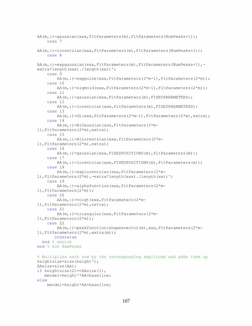
107

AA(m,:)=gaussian(xxx,FitParameters(m),FitParameters(NumPeaks+1)); case 7

AA(m,:)=lorentzian(xxx,FitParameters(m),FitParameters(NumPeaks+1)); case 8

AA(m,:)=expgaussian(xxx,FitParameters(m),FitParameters(NumPeaks+1),-

extra*length(xxx)./length(xx))'; case 9 AA(m,:)=exppulse(xxx,FitParameters(2*m-1),FitParameters(2*m)); case 10 AA(m,:)=sigmoid(xxx,FitParameters(2*m-1),FitParameters(2*m)); case 11 AA(m,:)=gaussian(xxx,FitParameters(m),FIXEDPARAMETERS); case 12 AA(m,:)=lorentzian(xxx,FitParameters(m),FIXEDPARAMETERS); case 13 AA(m,:)=GL(xxx,FitParameters(2*m-1),FitParameters(2*m),extra); case 14 AA(m,:)=BiGaussian(xxx,FitParameters(2*m-

1),FitParameters(2*m),extra); case 15 AA(m,:)=BiLorentzian(xxx,FitParameters(2*m-

1),FitParameters(2*m),extra); case 16 AA(m,:)=gaussian(xxx,FIXEDPOSITIONS(m),FitParameters(m)); case 17 AA(m,:)=lorentzian(xxx,FIXEDPOSITIONS(m),FitParameters(m)); case 18 AA(m,:)=explorentzian(xxx,FitParameters(2*m-

1),FitParameters(2*m),-extra*length(xxx)./length(xx))'; case 19 AA(m,:)=alphafunction(xxx,FitParameters(2*m-

1),FitParameters(2*m)); case 20 AA(m,:)=voigt(xxx,FitParameters(2*m-

1),FitParameters(2*m),extra); case 21 AA(m,:)=triangular(xxx,FitParameters(2*m-

1),FitParameters(2*m)); case 22 AA(m,:)=peakfunction(shapesvector(m),xxx,FitParameters(2*m-

1),FitParameters(2*m),extra(m)); otherwise end % switch end % for NumPeaks

% Multiplies each row by the corresponding amplitude and adds them up heightsize=size(height'); AAsize=size(AA); if heightsize(2)==AAsize(1), mmodel=height'*AA+baseline; else mmodel=height*AA+baseline;

108

end % Top half of the figure shows original signal and the fitted model. if plots, subplot(2,1,1);plot(xx+xoffset,yy,'b.'); % Plot the original signal

in blue dots hold on end for m=1:NumPeaks, if plots, plot(xxx+xoffset,height(m)*AA(m,:)+baseline,'g'),end %

Plot the individual component peaks in green lines area(m)=trapz(xxx+xoffset,height(m)*AA(m,:)); % Compute the area of

each component peak using trapezoidal method yi(m,:)=height(m)*AA(m,:); % (NEW) Place y values of individual

model peaks into matrix yi end xi=xxx+xoffset; % (NEW) Place the x-values of the individual model

peaks into xi

if plots, % Mark starting peak positions with vertical dashed lines if peakshape(1)==16||peakshape(1)==17 else for marker=1:NumPeaks, markx=BestStart((2*marker)-1); subplot(2,1,1);plot([markx+xoffset markx+xoffset],[0

max(yy)],'m--') end % for end % if peakshape plot(xxx+xoffset,mmodel,'r'); % Plot the total model (sum of

component peaks) in red lines hold off; lyy=min(yy); uyy=max(yy)+(max(yy)-min(yy))/10; if BIPOLAR, axis([min(xx) max(xx) lyy uyy]); ylabel('+ - mode') else axis([min(xx) max(xx) 0 uyy]); ylabel('+ mode') end switch AUTOZERO, case 0 title(['peakfit 5.1 No baseline correction']) case 1 title(['peakfit 5.1 Linear baseline subtraction']) case 2 title(['peakfit 5.1 Quadratic subtraction baseline']) case 3 title(['peakfit 5.1 Flat baseline correction']) end

switch peakshape(1) case {4,20}

109

xlabel(['Peaks = ' num2str(NumPeaks) ' Shape = '

ShapeString ' Shape Constant = ' num2str(extra) ' Error = '

num2str(round(1000*LowestError)/1000) '%' ] ) case {5,8,18} xlabel(['Peaks = ' num2str(NumPeaks) ' Shape = '

ShapeString ' Time Constant = ' num2str(extra) ' Error = '

num2str(round(1000*LowestError)/1000) '%' ] ) case 13 xlabel(['Peaks = ' num2str(NumPeaks) ' Shape = '

ShapeString ' % Gaussian = ' num2str(extra) ' Error = '

num2str(round(1000*LowestError)/1000) '% ' ] ) case {14,15,22} xlabel(['Peaks = ' num2str(NumPeaks) ' Shape = '

ShapeString ' extra = ' num2str(extra) ' Error = '

num2str(round(1000*LowestError)/1000) '% ' ] ) otherwise xlabel(['Peaks = ' num2str(NumPeaks) ' Shape = '

ShapeString ' Error = ' num2str(round(1000*LowestError)/1000) '% '

] ) end

% Bottom half of the figure shows the residuals and displays RMS

error % between original signal and model residual=yy-bestmodel; subplot(2,1,2);plot(xx+xoffset,residual,'b.') axis([min(xx)+xoffset max(xx)+xoffset min(residual)

max(residual)]); xlabel('Residual Plot') end % if plots

% Put results into a matrix, one row for each peak, showing peak index

number, % position, amplitude, and width. for m=1:NumPeaks, if m==1, if peakshape(1)==6||peakshape(1)==7||peakshape(1)==8, % equal-

width peak models only FitResults=[[round(m) FitParameters(m)+xoffset height(m)

abs(FitParameters(NumPeaks+1)) area(m)]]; else if peakshape(1)==11||peakshape(1)==12, % Fixed-width shapes

only FitResults=[[round(m) FitParameters(m)+xoffset

height(m) FIXEDPARAMETERS area(m)]]; else if peakshape(1)==16||peakshape(1)==17, % Fixed-position

shapes only FitResults=[round(m) FIXEDPOSITIONS(m) height(m)

FitParameters(m) area(m)]; else FitResults=[round(m) FitParameters(2*m-1)+xoffset

height(m) abs(FitParameters(2*m)) area(m)]; end end

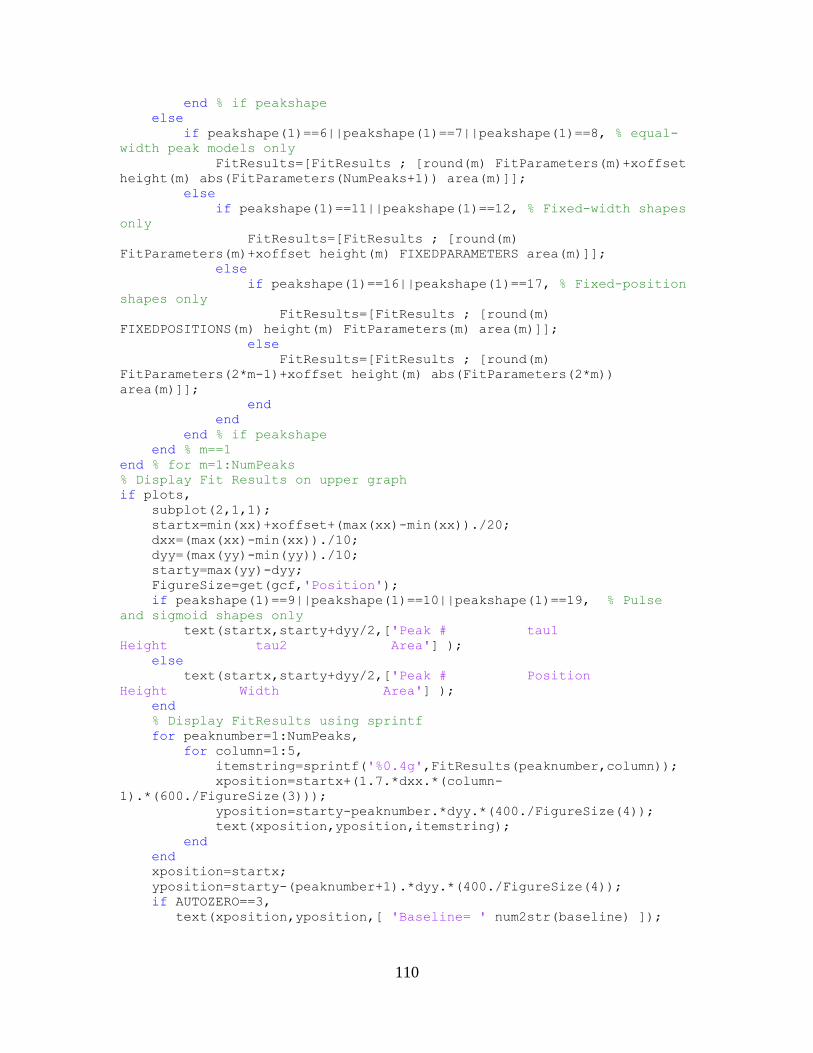
110

end % if peakshape else if peakshape(1)==6||peakshape(1)==7||peakshape(1)==8, % equal-

width peak models only FitResults=[FitResults ; [round(m) FitParameters(m)+xoffset

height(m) abs(FitParameters(NumPeaks+1)) area(m)]]; else if peakshape(1)==11||peakshape(1)==12, % Fixed-width shapes

only FitResults=[FitResults ; [round(m)

FitParameters(m)+xoffset height(m) FIXEDPARAMETERS area(m)]]; else if peakshape(1)==16||peakshape(1)==17, % Fixed-position

shapes only FitResults=[FitResults ; [round(m)

FIXEDPOSITIONS(m) height(m) FitParameters(m) area(m)]]; else FitResults=[FitResults ; [round(m)

FitParameters(2*m-1)+xoffset height(m) abs(FitParameters(2*m))

area(m)]]; end end end % if peakshape end % m==1 end % for m=1:NumPeaks % Display Fit Results on upper graph if plots, subplot(2,1,1); startx=min(xx)+xoffset+(max(xx)-min(xx))./20; dxx=(max(xx)-min(xx))./10; dyy=(max(yy)-min(yy))./10; starty=max(yy)-dyy; FigureSize=get(gcf,'Position'); if peakshape(1)==9||peakshape(1)==10||peakshape(1)==19, % Pulse

and sigmoid shapes only text(startx,starty+dyy/2,['Peak # tau1

Height tau2 Area'] ); else text(startx,starty+dyy/2,['Peak # Position

Height Width Area'] ); end % Display FitResults using sprintf for peaknumber=1:NumPeaks, for column=1:5, itemstring=sprintf('%0.4g',FitResults(peaknumber,column)); xposition=startx+(1.7.*dxx.*(column-

1).*(600./FigureSize(3))); yposition=starty-peaknumber.*dyy.*(400./FigureSize(4)); text(xposition,yposition,itemstring); end end xposition=startx; yposition=starty-(peaknumber+1).*dyy.*(400./FigureSize(4)); if AUTOZERO==3, text(xposition,yposition,[ 'Baseline= ' num2str(baseline) ]);

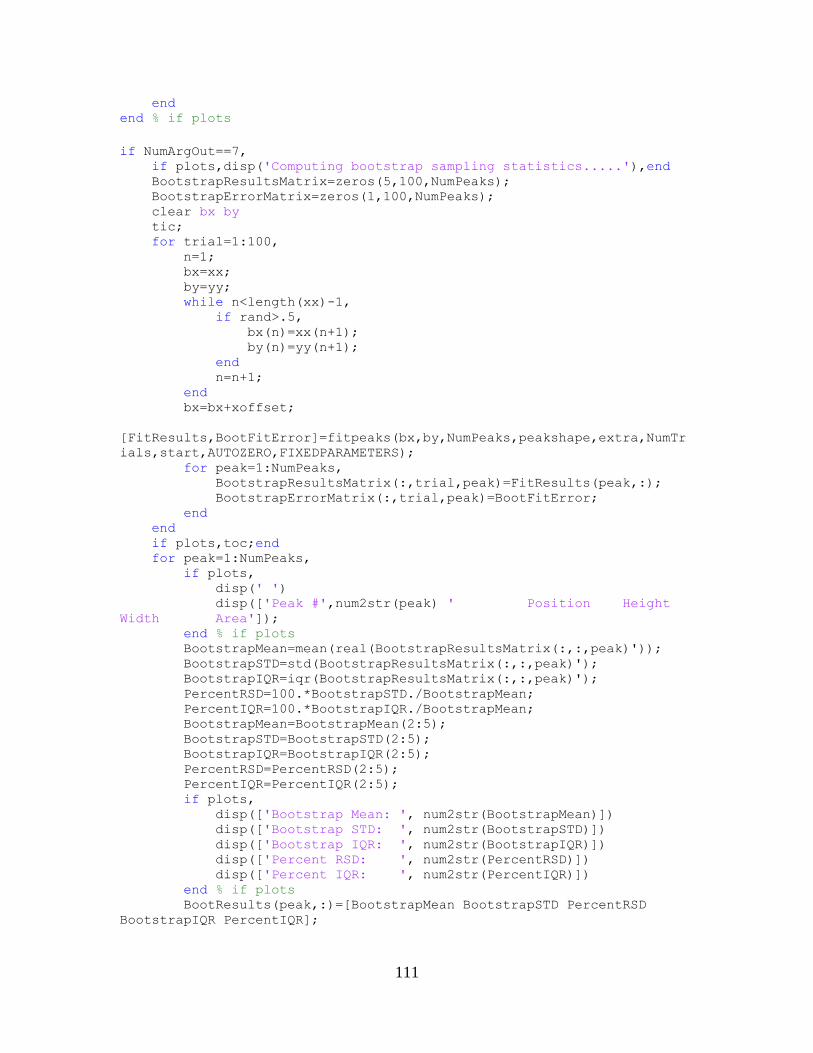
111

end end % if plots

if NumArgOut==7, if plots,disp('Computing bootstrap sampling statistics.....'),end BootstrapResultsMatrix=zeros(5,100,NumPeaks); BootstrapErrorMatrix=zeros(1,100,NumPeaks); clear bx by tic; for trial=1:100, n=1; bx=xx; by=yy; while n<length(xx)-1, if rand>.5, bx(n)=xx(n+1); by(n)=yy(n+1); end n=n+1; end bx=bx+xoffset;

[FitResults,BootFitError]=fitpeaks(bx,by,NumPeaks,peakshape,extra,NumTr

ials,start,AUTOZERO,FIXEDPARAMETERS); for peak=1:NumPeaks, BootstrapResultsMatrix(:,trial,peak)=FitResults(peak,:); BootstrapErrorMatrix(:,trial,peak)=BootFitError; end end if plots,toc;end for peak=1:NumPeaks, if plots, disp(' ') disp(['Peak #',num2str(peak) ' Position Height

Width Area']); end % if plots BootstrapMean=mean(real(BootstrapResultsMatrix(:,:,peak)')); BootstrapSTD=std(BootstrapResultsMatrix(:,:,peak)'); BootstrapIQR=iqr(BootstrapResultsMatrix(:,:,peak)'); PercentRSD=100.*BootstrapSTD./BootstrapMean; PercentIQR=100.*BootstrapIQR./BootstrapMean; BootstrapMean=BootstrapMean(2:5); BootstrapSTD=BootstrapSTD(2:5); BootstrapIQR=BootstrapIQR(2:5); PercentRSD=PercentRSD(2:5); PercentIQR=PercentIQR(2:5); if plots, disp(['Bootstrap Mean: ', num2str(BootstrapMean)]) disp(['Bootstrap STD: ', num2str(BootstrapSTD)]) disp(['Bootstrap IQR: ', num2str(BootstrapIQR)]) disp(['Percent RSD: ', num2str(PercentRSD)]) disp(['Percent IQR: ', num2str(PercentIQR)]) end % if plots BootResults(peak,:)=[BootstrapMean BootstrapSTD PercentRSD

BootstrapIQR PercentIQR];

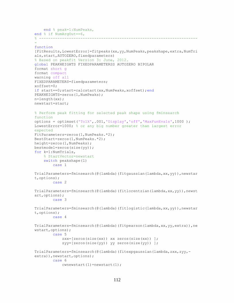
112

end % peak=1:NumPeaks, end % if NumArgOut==6, % ---------------------------------------------------------------------

- function

[FitResults,LowestError]=fitpeaks(xx,yy,NumPeaks,peakshape,extra,NumTri

als,start,AUTOZERO,fixedparameters) % Based on peakfit Version 3: June, 2012. global PEAKHEIGHTS FIXEDPARAMETERSS AUTOZERO BIPOLAR format short g format compact warning off all FIXEDPARAMETERS=fixedparameters; xoffset=0; if start==0;start=calcstart(xx,NumPeaks,xoffset);end PEAKHEIGHTS=zeros(1,NumPeaks); n=length(xx); newstart=start;

% Perform peak fitting for selected peak shape using fminsearch

function options = optimset('TolX',.001,'Display','off','MaxFunEvals',1000 ); LowestError=1000; % or any big number greater than largest error

expected FitParameters=zeros(1,NumPeaks.*2); BestStart=zeros(1,NumPeaks.*2); height=zeros(1,NumPeaks); bestmodel=zeros(size(yy)); for k=1:NumTrials, % StartVector=newstart switch peakshape(1) case 1

TrialParameters=fminsearch(@(lambda)(fitgaussian(lambda,xx,yy)),newstar

t,options); case 2

TrialParameters=fminsearch(@(lambda)(fitlorentzian(lambda,xx,yy)),newst


TrialParameters=fminsearch(@(lambda)(fitlogistic(lambda,xx,yy)),newstar

t,options); case 4

TrialParameters=fminsearch(@(lambda)(fitpearson(lambda,xx,yy,extra)),ne

wstart,options); case 5 zxx=[zeros(size(xx)) xx zeros(size(xx)) ]; zyy=[zeros(size(yy)) yy zeros(size(yy)) ];

TrialParameters=fminsearch(@(lambda)(fitexpgaussian(lambda,zxx,zyy,-

extra)),newstart,options); case 6 cwnewstart(1)=newstart(1);

113

for pc=2:NumPeaks, cwnewstart(pc)=newstart(2.*pc-1); end cwnewstart(NumPeaks+1)=(max(xx)-min(xx))/5;

TrialParameters=fminsearch(@(lambda)(fitewgaussian(lambda,xx,yy)),cwnew

start,options); case 7 cwnewstart(1)=newstart(1); for pc=2:NumPeaks, cwnewstart(pc)=newstart(2.*pc-1); end cwnewstart(NumPeaks+1)=(max(xx)-min(xx))/5;

TrialParameters=fminsearch(@(lambda)(fitewlorentzian(lambda,xx,yy)),cwn

ewstart,options); case 8 cwnewstart(1)=newstart(1); for pc=2:NumPeaks, cwnewstart(pc)=newstart(2.*pc-1); end cwnewstart(NumPeaks+1)=(max(xx)-min(xx))/5;

TrialParameters=fminsearch(@(lambda)(fitexpewgaussian(lambda,xx,yy,-

extra)),cwnewstart,options); case 9

TrialParameters=fminsearch(@(lambda)(fitexppulse(lambda,xx,yy)),newstar

t,options); case 10

TrialParameters=fminsearch(@(lambda)(fitsigmoid(lambda,xx,yy)),newstar,

optionst); case 11 fixedstart=[]; for pc=1:NumPeaks, fixedstart(pc)=min(xx)+pc.*(max(xx)-


TrialParameters=fminsearch(@(lambda)(FitFWGaussian(lambda,xx,yy)),fixed

start,options); case 12 fixedstart=[]; for pc=1:NumPeaks, fixedstart(pc)=min(xx)+pc.*(max(xx)-


TrialParameters=fminsearch(@(lambda)(FitFWLorentzian(lambda,xx,yy)),fix

edstart,options); case 13

TrialParameters=fminsearch(@(lambda)(fitGL(lambda,xx,yy,extra)),newstar

t,options);

114

case 14

TrialParameters=fminsearch(@(lambda)(fitBiGaussian(lambda,xx,yy,extra))

,newstart,options); case 15

TrialParameters=fminsearch(@(lambda)(fitBiLorentzian(lambda,xx,yy,extra

)),newstart,options); case 16 fixedstart=[]; for pc=1:NumPeaks, fixedstart(pc)=(max(xx)-min(xx))./(NumPeaks+1); end

TrialParameters=fminsearch(@(lambda)(FitFPGaussian(lambda,xx,yy)),fixed

start,options); case 17 fixedstart=[]; for pc=1:NumPeaks, fixedstart(pc)=(max(xx)-min(xx))./(NumPeaks+1); end

TrialParameters=fminsearch(@(lambda)(FitFPLorentzian(lambda,xx,yy)),fix

edstart,options); case 18 zxx=[zeros(size(xx)) xx zeros(size(xx)) ]; zyy=[zeros(size(yy)) yy zeros(size(yy)) ];

TrialParameters=fminsearch(@(lambda)(fitlorentzian(lambda,zxx,zyy,-

extra)),newstart,options); case 19

TrialParameters=fminsearch(@(lambda)(alphafunction(lambda,xx,yy)),newst


TrialParameters=fminsearch(@(lambda)(fitvoigt(lambda,xx,yy,extra)),news

tart,options); case 21

TrialParameters=fminsearch(@(lambda)(fittriangular(lambda,xx,yy)),newst


TrialParameters=fminsearch(@(lambda)(fitmultiple(lambda,xx,yy,shapesvec

tor,extra)),newstart,options); otherwise end % switch peakshape

for peaks=1:NumPeaks, peakindex=2*peaks-1; newstart(peakindex)=start(peakindex)-xoffset; end

115

% Construct model from Trial parameters A=zeros(NumPeaks,n); for m=1:NumPeaks, switch peakshape(1) case 1 A(m,:)=gaussian(xx,TrialParameters(2*m-

1),TrialParameters(2*m)); case 2 A(m,:)=lorentzian(xx,TrialParameters(2*m-

1),TrialParameters(2*m)); case 3 A(m,:)=logistic(xx,TrialParameters(2*m-

1),TrialParameters(2*m)); case 4 A(m,:)=pearson(xx,TrialParameters(2*m-

1),TrialParameters(2*m),extra); case 5 A(m,:)=expgaussian(xx,TrialParameters(2*m-

1),TrialParameters(2*m),-extra)'; case 6

A(m,:)=gaussian(xx,TrialParameters(m),TrialParameters(NumPeaks+1)); case 7

A(m,:)=lorentzian(xx,TrialParameters(m),TrialParameters(NumPeaks+1)); case 8

A(m,:)=expgaussian(xx,TrialParameters(m),TrialParameters(NumPeaks+1),-

extra)'; case 9 A(m,:)=exppulse(xx,TrialParameters(2*m-

1),TrialParameters(2*m)); case 10 A(m,:)=sigmoid(xx,TrialParameters(2*m-

1),TrialParameters(2*m)); case 11 A(m,:)=gaussian(xx,TrialParameters(m),FIXEDPARAMETERS); case 12

A(m,:)=lorentzian(xx,TrialParameters(m),FIXEDPARAMETERS); case 13 A(m,:)=GL(xx,TrialParameters(2*m-

1),TrialParameters(2*m),extra); case 14 A(m,:)=BiGaussian(xx,TrialParameters(2*m-

1),TrialParameters(2*m),extra); case 15 A(m,:)=BiLorentzian(xx,TrialParameters(2*m-

1),TrialParameters(2*m),extra); case 16

A(m,:)=gaussian(xx,FIXEDPOSITIONS(m),TrialParameters(m)); case 17

A(m,:)=lorentzian(xx,FIXEDPOSITIONS(m),TrialParameters(m));

116

case 18 A(m,:)=explorentzian(xx,TrialParameters(2*m-

1),TrialParameters(2*m),-extra)'; case 19 A(m,:)=alphafunction(xx,TrialParameters(2*m-

1),TrialParameters(2*m)); case 20 A(m,:)=voigt(xx,TrialParameters(2*m-

1),TrialParameters(2*m),extra); case 21 A(m,:)=triangular(xx,TrialParameters(2*m-

1),TrialParameters(2*m)); case 22

A(m,:)=peakfunction(shapesvector(m),xx,TrialParameters(2*m-

1),TrialParameters(2*m),extra(m)); end % switch % for parameter=1:2:2*NumPeaks, % newstart(parameter)=newstart(parameter)*(1+(rand-

.5)/50); % newstart(parameter+1)=newstart(parameter+1)*(1+(rand-

.5)/10); % end end % for

% Multiplies each row by the corresponding amplitude and adds them

up if AUTOZERO==3, baseline=PEAKHEIGHTS(1); Heights=PEAKHEIGHTS(2:1+NumPeaks); model=Heights'*A+baseline; else model=PEAKHEIGHTS'*A; Heights=PEAKHEIGHTS; baseline=0; end

% Compare trial model to data segment and compute the fit error MeanFitError=100*norm(yy-model)./(sqrt(n)*max(yy)); % Take only the single fit that has the lowest MeanFitError if MeanFitError<LowestError, if min(Heights)>=-BIPOLAR*10^100, % Consider only fits with

positive peak heights LowestError=MeanFitError; % Assign LowestError to the

lowest MeanFitError FitParameters=TrialParameters; % Assign FitParameters to

the fit with the lowest MeanFitError height=Heights; % Assign height to the PEAKHEIGHTS with the

lowest MeanFitError end % if min(PEAKHEIGHTS)>0 end % if MeanFitError<LowestError end % for k (NumTrials)

for m=1:NumPeaks,

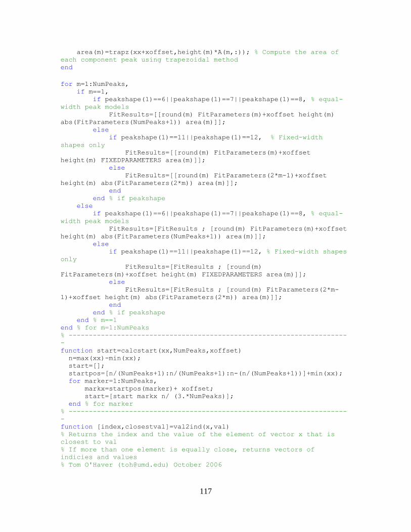
117

area(m)=trapz(xx+xoffset,height(m)*A(m,:)); % Compute the area of

each component peak using trapezoidal method end

for m=1:NumPeaks, if m==1, if peakshape(1)==6||peakshape(1)==7||peakshape(1)==8, % equal-

width peak models FitResults=[[round(m) FitParameters(m)+xoffset height(m)

abs(FitParameters(NumPeaks+1)) area(m)]]; else if peakshape(1)==11||peakshape(1)==12, % Fixed-width

shapes only FitResults=[[round(m) FitParameters(m)+xoffset

height(m) FIXEDPARAMETERS area(m)]]; else FitResults=[[round(m) FitParameters(2*m-1)+xoffset

height(m) abs(FitParameters(2*m)) area(m)]]; end end % if peakshape else if peakshape(1)==6||peakshape(1)==7||peakshape(1)==8, % equal-

width peak models FitResults=[FitResults ; [round(m) FitParameters(m)+xoffset

height(m) abs(FitParameters(NumPeaks+1)) area(m)]]; else if peakshape(1)==11||peakshape(1)==12, % Fixed-width shapes

only FitResults=[FitResults ; [round(m)

FitParameters(m)+xoffset height(m) FIXEDPARAMETERS area(m)]]; else FitResults=[FitResults ; [round(m) FitParameters(2*m-

1)+xoffset height(m) abs(FitParameters(2*m)) area(m)]]; end end % if peakshape end % m==1 end % for m=1:NumPeaks % ---------------------------------------------------------------------

- function start=calcstart(xx,NumPeaks,xoffset) n=max(xx)-min(xx); start=[]; startpos=[n/(NumPeaks+1):n/(NumPeaks+1):n-(n/(NumPeaks+1))]+min(xx); for marker=1:NumPeaks, markx=startpos(marker)+ xoffset; start=[start markx n/ (3.*NumPeaks)]; end % for marker % ---------------------------------------------------------------------

- function [index,closestval]=val2ind(x,val) % Returns the index and the value of the element of vector x that is

closest to val % If more than one element is equally close, returns vectors of

indicies and values % Tom O'Haver ([email protected]) October 2006

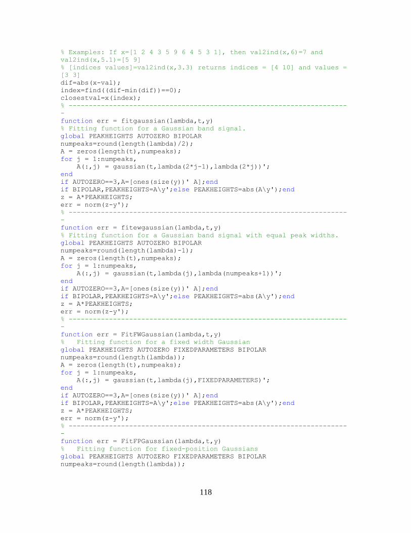
118

% Examples: If x=[1 2 4 3 5 9 6 4 5 3 1], then val2ind(x,6)=7 and

val2ind(x,5.1)=[5 9] % [indices values]=val2ind(x,3.3) returns indices = [4 10] and values =

[3 3] dif=abs(x-val); index=find((dif-min(dif))==0); closestval=x(index); % ---------------------------------------------------------------------

- function err = fitgaussian(lambda,t,y) % Fitting function for a Gaussian band signal. global PEAKHEIGHTS AUTOZERO BIPOLAR numpeaks=round(length(lambda)/2); A = zeros(length(t),numpeaks); for j = 1:numpeaks, A(:,j) = gaussian(t,lambda(2*j-1),lambda(2*j))'; end if AUTOZERO==3,A=[ones(size(y))' A];end if BIPOLAR,PEAKHEIGHTS=A\y';else PEAKHEIGHTS=abs(A\y');end z = A*PEAKHEIGHTS; err = norm(z-y'); % ---------------------------------------------------------------------

- function err = fitewgaussian(lambda,t,y) % Fitting function for a Gaussian band signal with equal peak widths. global PEAKHEIGHTS AUTOZERO BIPOLAR numpeaks=round(length(lambda)-1); A = zeros(length(t),numpeaks); for j = 1:numpeaks, A(:,j) = gaussian(t,lambda(j),lambda(numpeaks+1))'; end if AUTOZERO==3,A=[ones(size(y))' A];end if BIPOLAR,PEAKHEIGHTS=A\y';else PEAKHEIGHTS=abs(A\y');end z = A*PEAKHEIGHTS; err = norm(z-y'); % ---------------------------------------------------------------------

- function err = FitFWGaussian(lambda,t,y) % Fitting function for a fixed width Gaussian global PEAKHEIGHTS AUTOZERO FIXEDPARAMETERS BIPOLAR numpeaks=round(length(lambda)); A = zeros(length(t),numpeaks); for j = 1:numpeaks, A(:,j) = gaussian(t,lambda(j),FIXEDPARAMETERS)'; end if AUTOZERO==3,A=[ones(size(y))' A];end if BIPOLAR,PEAKHEIGHTS=A\y';else PEAKHEIGHTS=abs(A\y');end z = A*PEAKHEIGHTS; err = norm(z-y'); % ---------------------------------------------------------------------

- function err = FitFPGaussian(lambda,t,y) % Fitting function for fixed-position Gaussians global PEAKHEIGHTS AUTOZERO FIXEDPARAMETERS BIPOLAR numpeaks=round(length(lambda));

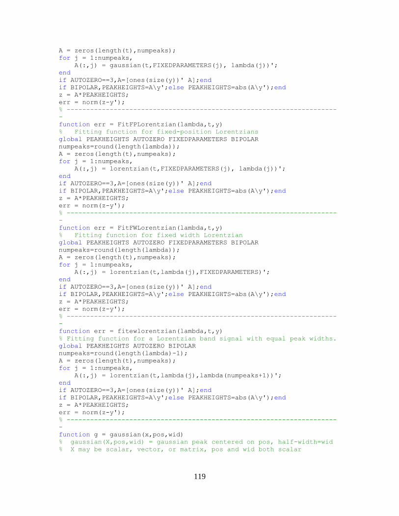
119

A = zeros(length(t),numpeaks); for j = 1:numpeaks, A(:,j) = gaussian(t,FIXEDPARAMETERS(j), lambda(j))'; end if AUTOZERO==3,A=[ones(size(y))' A];end if BIPOLAR,PEAKHEIGHTS=A\y';else PEAKHEIGHTS=abs(A\y');end z = A*PEAKHEIGHTS; err = norm(z-y'); % ---------------------------------------------------------------------

- function err = FitFPLorentzian(lambda,t,y) % Fitting function for fixed-position Lorentzians global PEAKHEIGHTS AUTOZERO FIXEDPARAMETERS BIPOLAR numpeaks=round(length(lambda)); A = zeros(length(t),numpeaks); for j = 1:numpeaks, A(:,j) = lorentzian(t,FIXEDPARAMETERS(j), lambda(j))'; end if AUTOZERO==3,A=[ones(size(y))' A];end if BIPOLAR,PEAKHEIGHTS=A\y';else PEAKHEIGHTS=abs(A\y');end z = A*PEAKHEIGHTS; err = norm(z-y'); % ---------------------------------------------------------------------

- function err = FitFWLorentzian(lambda,t,y) % Fitting function for fixed width Lorentzian global PEAKHEIGHTS AUTOZERO FIXEDPARAMETERS BIPOLAR numpeaks=round(length(lambda)); A = zeros(length(t),numpeaks); for j = 1:numpeaks, A(:,j) = lorentzian(t,lambda(j),FIXEDPARAMETERS)'; end if AUTOZERO==3,A=[ones(size(y))' A];end if BIPOLAR,PEAKHEIGHTS=A\y';else PEAKHEIGHTS=abs(A\y');end z = A*PEAKHEIGHTS; err = norm(z-y'); % ---------------------------------------------------------------------

- function err = fitewlorentzian(lambda,t,y) % Fitting function for a Lorentzian band signal with equal peak widths. global PEAKHEIGHTS AUTOZERO BIPOLAR numpeaks=round(length(lambda)-1); A = zeros(length(t),numpeaks); for j = 1:numpeaks, A(:,j) = lorentzian(t,lambda(j),lambda(numpeaks+1))'; end if AUTOZERO==3,A=[ones(size(y))' A];end if BIPOLAR,PEAKHEIGHTS=A\y';else PEAKHEIGHTS=abs(A\y');end z = A*PEAKHEIGHTS; err = norm(z-y'); % ---------------------------------------------------------------------

- function g = gaussian(x,pos,wid) % gaussian(X,pos,wid) = gaussian peak centered on pos, half-width=wid % X may be scalar, vector, or matrix, pos and wid both scalar

120

% Examples: gaussian([0 1 2],1,2) gives result [0.5000 1.0000

0.5000] % plot(gaussian([1:100],50,20)) displays gaussian band centered at 50

with width 20. g = exp(-((x-pos)./(0.6005615.*wid)).^2); % ---------------------------------------------------------------------

- function err = fitlorentzian(lambda,t,y) % Fitting function for single lorentzian, lambda(1)=position,

lambda(2)=width % Fitgauss assumes a lorentzian function global PEAKHEIGHTS AUTOZERO BIPOLAR A = zeros(length(t),round(length(lambda)/2)); for j = 1:length(lambda)/2, A(:,j) = lorentzian(t,lambda(2*j-1),lambda(2*j))'; end if AUTOZERO==3,A=[ones(size(y))' A];end if BIPOLAR,PEAKHEIGHTS=A\y';else PEAKHEIGHTS=abs(A\y');end z = A*PEAKHEIGHTS; err = norm(z-y'); % ---------------------------------------------------------------------

- function g = lorentzian(x,position,width) % lorentzian(x,position,width) Lorentzian function. % where x may be scalar, vector, or matrix % position and width scalar % T. C. O'Haver, 1988 % Example: lorentzian([1 2 3],2,2) gives result [0.5 1 0.5] g=ones(size(x))./(1+((x-position)./(0.5.*width)).^2); % ---------------------------------------------------------------------

- function err = fitlogistic(lambda,t,y) % Fitting function for logistic, lambda(1)=position, lambda(2)=width % between the data and the values computed by the current % function of lambda. Fitlogistic assumes a logistic function % T. C. O'Haver, May 2006 global PEAKHEIGHTS AUTOZERO BIPOLAR A = zeros(length(t),round(length(lambda)/2)); for j = 1:length(lambda)/2, A(:,j) = logistic(t,lambda(2*j-1),lambda(2*j))'; end if AUTOZERO==3,A=[ones(size(y))' A];end if BIPOLAR,PEAKHEIGHTS=A\y';else PEAKHEIGHTS=abs(A\y');end z = A*PEAKHEIGHTS; err = norm(z-y'); % ---------------------------------------------------------------------

- function g = logistic(x,pos,wid) % logistic function. pos=position; wid=half-width (both scalar) % logistic(x,pos,wid), where x may be scalar, vector, or matrix % pos=position; wid=half-width (both scalar) % T. C. O'Haver, 1991 n = exp(-((x-pos)/(.477.*wid)) .^2); g = (2.*n)./(1+n);

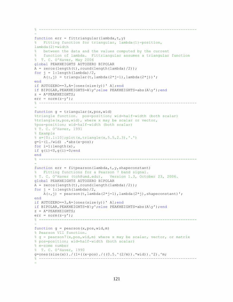
121

% ---------------------------------------------------------------------

- function err = fittriangular(lambda,t,y) % Fitting function for triangular, lambda(1)=position,

lambda(2)=width % between the data and the values computed by the current % function of lambda. Fittriangular assumes a triangular function % T. C. O'Haver, May 2006 global PEAKHEIGHTS AUTOZERO BIPOLAR A = zeros(length(t),round(length(lambda)/2)); for j = 1:length(lambda)/2, A(:,j) = triangular(t,lambda(2*j-1),lambda(2*j))'; end if AUTOZERO==3,A=[ones(size(y))' A];end if BIPOLAR,PEAKHEIGHTS=A\y';else PEAKHEIGHTS=abs(A\y');end z = A*PEAKHEIGHTS; err = norm(z-y'); % ---------------------------------------------------------------------

- function g = triangular(x,pos,wid) %triangle function. pos=position; wid=half-width (both scalar) %triangle(x,pos,wid), where x may be scalar or vector, %pos=position; wid=half-width (both scalar) % T. C. O'Haver, 1991 % Example % x=[0:.1:10];plot(x,triangle(x,5.5,2.3),'.') g=1-(1./wid) .*abs(x-pos); for i=1:length(x), if g(i)<0,g(i)=0;end end % ---------------------------------------------------------------------

- function err = fitpearson(lambda,t,y,shapeconstant) % Fitting functions for a Pearson 7 band signal. % T. C. O'Haver ([email protected]), Version 1.3, October 23, 2006. global PEAKHEIGHTS AUTOZERO BIPOLAR A = zeros(length(t),round(length(lambda)/2)); for j = 1:length(lambda)/2, A(:,j) = pearson(t,lambda(2*j-1),lambda(2*j),shapeconstant)'; end if AUTOZERO==3,A=[ones(size(y))' A];end if BIPOLAR,PEAKHEIGHTS=A\y';else PEAKHEIGHTS=abs(A\y');end z = A*PEAKHEIGHTS; err = norm(z-y'); % ---------------------------------------------------------------------

- function g = pearson(x,pos,wid,m) % Pearson VII function. % g = pearson7(x,pos,wid,m) where x may be scalar, vector, or matrix % pos=position; wid=half-width (both scalar) % m=some number % T. C. O'Haver, 1990 g=ones(size(x))./(1+((x-pos)./((0.5.^(2/m)).*wid)).^2).^m; % ---------------------------------------------------------------------

-

122

function err = fitexpgaussian(lambda,t,y,timeconstant) % Fitting functions for a exponentially-broadened Gaussian band

signal. % T. C. O'Haver, October 23, 2006. global PEAKHEIGHTS AUTOZERO BIPOLAR A = zeros(length(t),round(length(lambda)/2)); for j = 1:length(lambda)/2, A(:,j) = expgaussian(t,lambda(2*j-1),lambda(2*j),timeconstant); end if AUTOZERO==3,A=[ones(size(y))' A];end if BIPOLAR,PEAKHEIGHTS=A\y';else PEAKHEIGHTS=abs(A\y');end z = A*PEAKHEIGHTS; err = norm(z-y'); % ---------------------------------------------------------------------

- function err = fitexplorentzian(lambda,t,y,timeconstant) % Fitting functions for a exponentially-broadened lorentzian band

signal. % T. C. O'Haver, 2013. global PEAKHEIGHTS AUTOZERO BIPOLAR A = zeros(length(t),round(length(lambda)/2)); for j = 1:length(lambda)/2, A(:,j) = explorentzian(t,lambda(2*j-1),lambda(2*j),timeconstant); end if AUTOZERO==3,A=[ones(size(y))' A];end if BIPOLAR,PEAKHEIGHTS=A\y';else PEAKHEIGHTS=abs(A\y');end z = A*PEAKHEIGHTS; err = norm(z-y'); % ---------------------------------------------------------------------

- function err = fitexpewgaussian(lambda,t,y,timeconstant) % Fitting function for exponentially-broadened Gaussian bands with

equal peak widths. global PEAKHEIGHTS AUTOZERO BIPOLAR numpeaks=round(length(lambda)-1); A = zeros(length(t),numpeaks); for j = 1:numpeaks, A(:,j) = expgaussian(t,lambda(j),lambda(numpeaks+1),timeconstant); end if AUTOZERO==3,A=[ones(size(y))' A];end if BIPOLAR,PEAKHEIGHTS=A\y';else PEAKHEIGHTS=abs(A\y');end z = A*PEAKHEIGHTS; err = norm(z-y'); % ---------------------------------------------------------------------

- function g = expgaussian(x,pos,wid,timeconstant) % Exponentially-broadened gaussian(x,pos,wid) = gaussian peak centered

on pos, half-width=wid % x may be scalar, vector, or matrix, pos and wid both scalar % T. C. O'Haver, 2006 g = exp(-((x-pos)./(0.6005615.*wid)) .^2); g = ExpBroaden(g',timeconstant); % ---------------------------------------------------------------------

- function g = explorentzian(x,pos,wid,timeconstant)

123

% Exponentially-broadened lorentzian(x,pos,wid) = lorentzian peak

centered on pos, half-width=wid % x may be scalar, vector, or matrix, pos and wid both scalar % T. C. O'Haver, 2013 g = ones(size(x))./(1+((x-pos)./(0.5.*wid)).^2); g = ExpBroaden(g',timeconstant); % ---------------------------------------------------------------------

- function yb = ExpBroaden(y,t) % ExpBroaden(y,t) zero pads y and convolutes result by an exponential

decay % of time constant t by multiplying Fourier transforms and inverse % transforming the result. hly=round(length(y)./2); ey=[y(1).*ones(1,hly)';y;y(length(y)).*ones(1,hly)']; % figure(2);plot(ey);figure(1); fy=fft(ey); a=exp(-(1:length(fy))./t); fa=fft(a); fy1=fy.*fa'; ybz=real(ifft(fy1))./sum(a); yb=ybz(hly+2:length(ybz)-hly+1); % ---------------------------------------------------------------------

- function err = fitexppulse(tau,x,y) % Iterative fit of the sum of exponential pulses % of the form Height.*exp(-tau1.*x).*(1-exp(-tau2.*x))) global PEAKHEIGHTS AUTOZERO BIPOLAR A = zeros(length(x),round(length(tau)/2)); for j = 1:length(tau)/2, A(:,j) = exppulse(x,tau(2*j-1),tau(2*j)); end if AUTOZERO==3,A=[ones(size(y))' A];end if BIPOLAR,PEAKHEIGHTS=A\y';else PEAKHEIGHTS=abs(A\y');end z = A*PEAKHEIGHTS; err = norm(z-y'); % ---------------------------------------------------------------------

- function g = exppulse(x,t1,t2) % Exponential pulse of the form % g = (x-spoint)./pos.*exp(1-(x-spoint)./pos); e=(x-t1)./t2; p = 4*exp(-e).*(1-exp(-e)); p=p .* (p>0); g = p'; % ---------------------------------------------------------------------

- function err = fitalphafunction(tau,x,y) % Iterative fit of the sum of alpha funciton % of the form Height.*exp(-tau1.*x).*(1-exp(-tau2.*x))) global PEAKHEIGHTS AUTOZERO BIPOLAR A = zeros(length(x),round(length(tau)/2)); for j = 1:length(tau)/2, A(:,j) = alphafunction(x,tau(2*j-1),tau(2*j)); end

124

if AUTOZERO==3,A=[ones(size(y))' A];end if BIPOLAR,PEAKHEIGHTS=A\y';else PEAKHEIGHTS=abs(A\y');end z = A*PEAKHEIGHTS; err = norm(z-y'); % ---------------------------------------------------------------------

- function g = alphafunction(x,pos,spoint) % alpha function. pos=position; wid=half-width (both scalar) % alphafunction(x,pos,wid), where x may be scalar, vector, or matrix % pos=position; wid=half-width (both scalar) % Taekyung Kwon, July 2013 g = (x-spoint)./pos.*exp(1-(x-spoint)./pos); for m=1:length(x);if g(m)<0;g(m)=0;end;end % ---------------------------------------------------------------------

- function err = fitsigmoid(tau,x,y) % Fitting function for iterative fit to the sum of % sigmiods of the form Height./(1 + exp((t1 - t)/t2)) global PEAKHEIGHTS AUTOZERO BIPOLAR A = zeros(length(x),round(length(tau)/2)); for j = 1:length(tau)/2, A(:,j) = sigmoid(x,tau(2*j-1),tau(2*j)); end if AUTOZERO==3,A=[ones(size(y))' A];end if BIPOLAR,PEAKHEIGHTS=A\y';else PEAKHEIGHTS=abs(A\y');end z = A*PEAKHEIGHTS; err = norm(z-y'); % ---------------------------------------------------------------------

- function g=sigmoid(x,t1,t2) % g=1./(1 + exp((t1 - x)./t2))'; % old version of sigmoid g=1/2 + 1/2* erf(real((x-t1)/sqrt(2*t2))); % Modified sigmoid % Bifurcated sigmoid % lx=length(x); % hx=val2ind(x,t1); % g(1:hx)=1./(1 + exp((t1 - x(1:hx))./t2)); % g(hx+1:lx)=1./(1 + exp((t1 - x(hx+1:lx))./(1.3*t2))); % ---------------------------------------------------------------------

- function err = fitGL(lambda,t,y,shapeconstant) % Fitting functions for Gaussian/Lorentzian blend. % T. C. O'Haver ([email protected]), 2012. global PEAKHEIGHTS AUTOZERO BIPOLAR A = zeros(length(t),round(length(lambda)/2)); for j = 1:length(lambda)/2, A(:,j) = GL(t,lambda(2*j-1),lambda(2*j),shapeconstant)'; end if AUTOZERO==3,A=[ones(size(y))' A];end if BIPOLAR,PEAKHEIGHTS=A\y';else PEAKHEIGHTS=abs(A\y');end z = A*PEAKHEIGHTS; err = norm(z-y'); % ---------------------------------------------------------------------

- function g = GL(x,pos,wid,m) % Gaussian/Lorentzian blend. m = percent Gaussian character

125

% pos=position; wid=half-width % m = percent Gaussian character. % T. C. O'Haver, 2012 % sizex=size(x) % sizepos=size(pos) % sizewid=size(wid) % sizem=size(m) g=2.*((m/100).*gaussian(x,pos,wid)+(1-

(m(1)/100)).*lorentzian(x,pos,wid))/2; % ---------------------------------------------------------------------

- function err = fitvoigt(lambda,t,y,shapeconstant) % Fitting functions for Voigt profile function % T. C. O'Haver ([email protected]), 2013. global PEAKHEIGHTS AUTOZERO BIPOLAR A = zeros(length(t),round(length(lambda)/2)); for j = 1:length(lambda)/2, A(:,j) = voigt(t,lambda(2*j-1),lambda(2*j),shapeconstant)'; end if AUTOZERO==3,A=[ones(size(y))' A];end if BIPOLAR,PEAKHEIGHTS=A\y';else PEAKHEIGHTS=abs(A\y');end z = A*PEAKHEIGHTS; err = norm(z-y'); % ---------------------------------------------------------------------

- function g=voigt(xx,pos,gD,alpha) % Voigt profile function. xx is the independent variable (energy, % wavelength, etc), gD is the Doppler (Gaussian) width, and alpha is

the % shape constant (ratio of the Lorentzian width gL to the Doppler width

gD. % Based on Chong Tao's "Voigt lineshape spectrum simulation", % File ID: #26707 % alpha=alpha gL=alpha.*gD; gV = 0.5346*gL + sqrt(0.2166*gL.^2 + gD.^2); x = gL/gV; y = abs(xx-pos)/gV; g = 1/(2*gV*(1.065 + 0.447*x + 0.058*x^2))*((1-x)*exp(-0.693.*y.^2) +

(x./(1+y.^2)) + 0.016*(1-x)*x*(exp(-0.0841.*y.^2.25)-1./(1 +

0.021.*y.^2.25))); g=g./max(g); % ---------------------------------------------------------------------

- function err = fitBiGaussian(lambda,t,y,shapeconstant) % Fitting functions for BiGaussian. % T. C. O'Haver ([email protected]), 2012. global PEAKHEIGHTS AUTOZERO BIPOLAR A = zeros(length(t),round(length(lambda)/2)); for j = 1:length(lambda)/2, A(:,j) = BiGaussian(t,lambda(2*j-1),lambda(2*j),shapeconstant)'; end if AUTOZERO==3,A=[ones(size(y))' A];end if BIPOLAR,PEAKHEIGHTS=A\y';else PEAKHEIGHTS=abs(A\y');end z = A*PEAKHEIGHTS;

126

err = norm(z-y'); % ---------------------------------------------------------------------

- function g = BiGaussian(x,pos,wid,m) % BiGaussian (different widths on leading edge and trailing edge). % pos=position; wid=width % m determines shape; symmetrical if m=50. % T. C. O'Haver, 2012 lx=length(x); hx=val2ind(x,pos); g(1:hx)=gaussian(x(1:hx),pos,wid*(m/100)); g(hx+1:lx)=gaussian(x(hx+1:lx),pos,wid*(1-m/100)); % ---------------------------------------------------------------------

- function err = fitBiLorentzian(lambda,t,y,shapeconstant) % Fitting functions for BiGaussian. % T. C. O'Haver ([email protected]), 2012. global PEAKHEIGHTS AUTOZERO BIPOLAR A = zeros(length(t),round(length(lambda)/2)); for j = 1:length(lambda)/2, A(:,j) = BiLorentzian(t,lambda(2*j-1),lambda(2*j),shapeconstant)'; end if AUTOZERO==3,A=[ones(size(y))' A];end if BIPOLAR,PEAKHEIGHTS=A\y';else PEAKHEIGHTS=abs(A\y');end z = A*PEAKHEIGHTS; err = norm(z-y'); % ---------------------------------------------------------------------

- function g = BiLorentzian(x,pos,wid,m) % BiLorentzian (different widths on leading edge and trailing edge). % pos=position; wid=width % m determines shape; symmetrical if m=50. % T. C. O'Haver, 2012 lx=length(x); hx=val2ind(x,pos); g(1:hx)=lorentzian(x(1:hx),pos,wid*(m/100)); g(hx+1:lx)=lorentzian(x(hx+1:lx),pos,wid*(1-m/100)); % ---------------------------------------------------------------------

- function b=iqr(a) % b = IQR(a) returns the interquartile range of the values in a. For % vector input, b is the difference between the 75th and 25th

percentiles % of a. For matrix input, b is a row vector containing the

interquartile % range of each column of a. % T. C. O'Haver, 2012 mina=min(a); sizea=size(a); NumCols=sizea(2); for n=1:NumCols,b(:,n)=a(:,n)-mina(n);end Sorteda=sort(b); lx=length(Sorteda); SecondQuartile=round(lx/4); FourthQuartile=3*round(lx/4);

127

b=abs(Sorteda(FourthQuartile,:)-Sorteda(SecondQuartile,:)); % ---------------------------------------------------------------------

- function err = fitmultiple(lambda,t,y,shapesvector,m) % Fitting function for a multiple-shape band signal. % The sequence of peak shapes are defined by the vector "shape". % The vector "m" determines the shape of variable-shape peaks. global PEAKHEIGHTS AUTOZERO BIPOLAR numpeaks=round(length(lambda)/2); A = zeros(length(t),numpeaks); for j = 1:numpeaks, A(:,j) = peakfunction(shapesvector(j),t,lambda(2*j-

1),lambda(2*j),m(j))'; end if AUTOZERO==3,A=[ones(size(y))' A];end if BIPOLAR,PEAKHEIGHTS=A\y';else PEAKHEIGHTS=abs(A\y');end z = A*PEAKHEIGHTS; err = norm(z-y'); % ---------------------------------------------------------------------

- function p=peakfunction(shape,x,pos,wid,m) switch shape, case 1 p=gaussian(x,pos,wid); case 2 p=lorentzian(x,pos,wid); case 3 p=logistic(x,pos,wid); case 4 p=pearson(x,pos,wid,m); case 5 p=expgaussian(x,pos,wid,m)'; case 6 p=gaussian(x,pos,wid); case 7 p=lorentzian(x,pos,wid); case 8 p=expgaussian(x,pos,wid,m)'; case 9 p=exppulse(x,pos,wid); case 10 p=sigmoid(x,pos,wid); case 11 p=gaussian(x,pos,wid); case 12 p=lorentzian(x,pos,wid); case 13 p=GL(x,pos,wid,m); case 14 p=BiGaussian(x,pos,wid,m); case 15 p=BiLorentzian(x,pos,wid,m); case 16 p=gaussian(x,pos,wid); case 17

128

p=lorentzian(x,pos,wid); case 18 p=explorentzian(x,pos,wid,m)'; case 19 p=alphafunction(x,pos,wid); case 20 p=voigt(x,pos,wid,m); case 21 p=triangular(x,pos,wid); otherwise end % switch

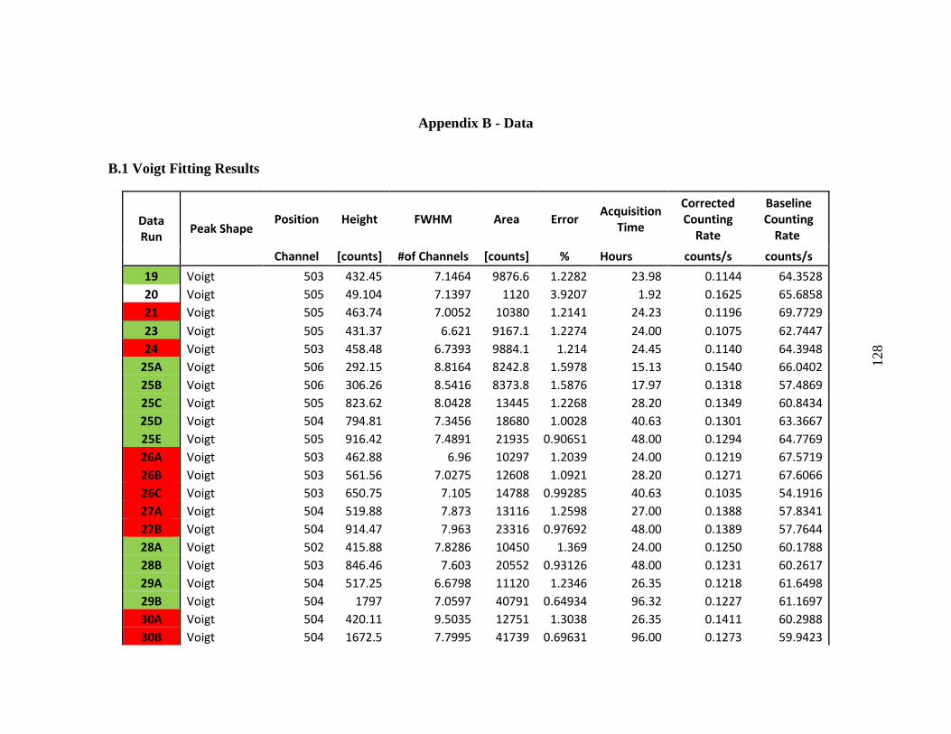
128

Appendix B - Data

B.1 Voigt Fitting Results

Data Run

Peak Shape Position Height FWHM Area Error

Acquisition Time

Corrected Counting

Rate

Baseline Counting

Rate

Channel [counts] #of Channels [counts] % Hours counts/s counts/s

19 Voigt 503 432.45 7.1464 9876.6 1.2282 23.98 0.1144 64.3528

20 Voigt 505 49.104 7.1397 1120 3.9207 1.92 0.1625 65.6858

21 Voigt 505 463.74 7.0052 10380 1.2141 24.23 0.1196 69.7729

23 Voigt 505 431.37 6.621 9167.1 1.2274 24.00 0.1075 62.7447

24 Voigt 503 458.48 6.7393 9884.1 1.214 24.45 0.1140 64.3948

25A Voigt 506 292.15 8.8164 8242.8 1.5978 15.13 0.1540 66.0402

25B Voigt 506 306.26 8.5416 8373.8 1.5876 17.97 0.1318 57.4869

25C Voigt 505 823.62 8.0428 13445 1.2268 28.20 0.1349 60.8434

25D Voigt 504 794.81 7.3456 18680 1.0028 40.63 0.1301 63.3667

25E Voigt 505 916.42 7.4891 21935 0.90651 48.00 0.1294 64.7769

26A Voigt 503 462.88 6.96 10297 1.2039 24.00 0.1219 67.5719

26B Voigt 503 561.56 7.0275 12608 1.0921 28.20 0.1271 67.6066

26C Voigt 503 650.75 7.105 14788 0.99285 40.63 0.1035 54.1916

27A Voigt 504 519.88 7.873 13116 1.2598 27.00 0.1388 57.8341

27B Voigt 504 914.47 7.963 23316 0.97692 48.00 0.1389 57.7644

28A Voigt 502 415.88 7.8286 10450 1.369 24.00 0.1250 60.1788

28B Voigt 503 846.46 7.603 20552 0.93126 48.00 0.1231 60.2617

29A Voigt 504 517.25 6.6798 11120 1.2346 26.35 0.1218 61.6498

29B Voigt 504 1797 7.0597 40791 0.64934 96.32 0.1227 61.1697

30A Voigt 504 420.11 9.5035 12751 1.3038 26.35 0.1411 60.2988

30B Voigt 504 1672.5 7.7995 41739 0.69631 96.00 0.1273 59.9423

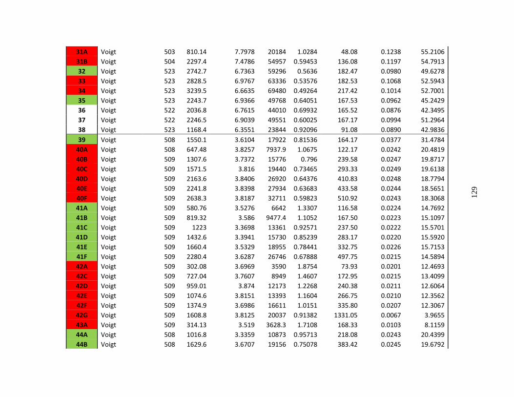
129

31A Voigt 503 810.14 7.7978 20184 1.0284 48.08 0.1238 55.2106

31B Voigt 504 2297.4 7.4786 54957 0.59453 136.08 0.1197 54.7913

32 Voigt 523 2742.7 6.7363 59296 0.5636 182.47 0.0980 49.6278

33 Voigt 523 2828.5 6.9767 63336 0.53576 182.53 0.1068 52.5943

34 Voigt 523 3239.5 6.6635 69480 0.49264 217.42 0.1014 52.7001

35 Voigt 523 2243.7 6.9366 49768 0.64051 167.53 0.0962 45.2429

36 Voigt 522 2036.8 6.7615 44010 0.69932 165.52 0.0876 42.3495

37 Voigt 522 2246.5 6.9039 49551 0.60025 167.17 0.0994 51.2964

38 Voigt 523 1168.4 6.3551 23844 0.92096 91.08 0.0890 42.9836

39 Voigt 508 1550.1 3.6104 17922 0.81536 164.17 0.0377 31.4784

40A Voigt 508 647.48 3.8257 7937.9 1.0675 122.17 0.0242 20.4819

40B Voigt 509 1307.6 3.7372 15776 0.796 239.58 0.0247 19.8717

40C Voigt 509 1571.5 3.816 19440 0.73465 293.33 0.0249 19.6138

40D Voigt 509 2163.6 3.8406 26920 0.64376 410.83 0.0248 18.7794

40E Voigt 509 2241.8 3.8398 27934 0.63683 433.58 0.0244 18.5651

40F Voigt 509 2638.3 3.8187 32711 0.59823 510.92 0.0243 18.3068

41A Voigt 509 580.76 3.5276 6642 1.3307 116.58 0.0224 14.7692

41B Voigt 509 819.32 3.586 9477.4 1.1052 167.50 0.0223 15.1097

41C Voigt 509 1223 3.3698 13361 0.92571 237.50 0.0222 15.5701

41D Voigt 509 1432.6 3.3941 15730 0.85239 283.17 0.0220 15.5920

41E Voigt 509 1660.4 3.5329 18955 0.78441 332.75 0.0226 15.7153

41F Voigt 509 2280.4 3.6287 26746 0.67888 497.75 0.0215 14.5894

42A Voigt 509 302.08 3.6969 3590 1.8754 73.93 0.0201 12.4693

42C Voigt 509 727.04 3.7607 8949 1.4607 172.95 0.0215 13.4099

42D Voigt 509 959.01 3.874 12173 1.2268 240.38 0.0211 12.6064

42E Voigt 509 1074.6 3.8151 13393 1.1604 266.75 0.0210 12.3562

42F Voigt 509 1374.9 3.6986 16611 1.0151 335.80 0.0207 12.3067

42G Voigt 509 1608.8 3.8125 20037 0.91382 1331.05 0.0067 3.9655

43A Voigt 509 314.13 3.519 3628.3 1.7108 168.33 0.0103 8.1159

44A Voigt 508 1016.8 3.3359 10873 0.95713 218.08 0.0243 20.4399

44B Voigt 508 1629.6 3.6707 19156 0.75078 383.42 0.0245 19.6792

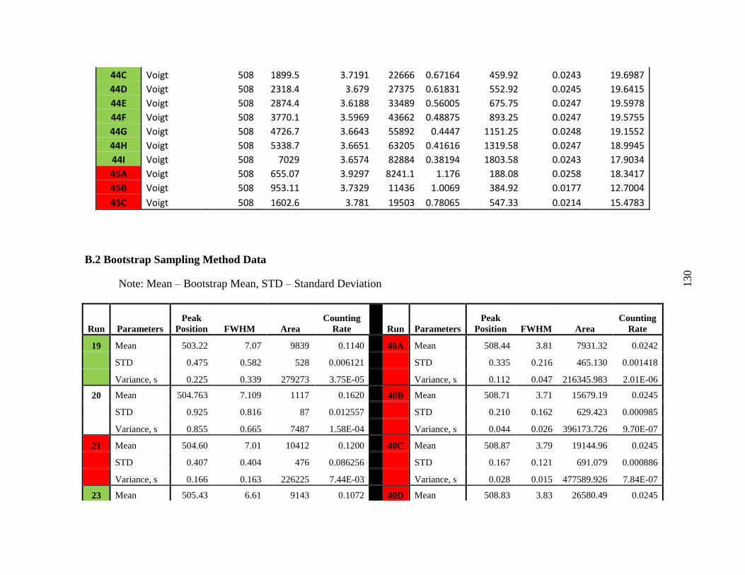
130

44C Voigt 508 1899.5 3.7191 22666 0.67164 459.92 0.0243 19.6987

44D Voigt 508 2318.4 3.679 27375 0.61831 552.92 0.0245 19.6415

44E Voigt 508 2874.4 3.6188 33489 0.56005 675.75 0.0247 19.5978

44F Voigt 508 3770.1 3.5969 43662 0.48875 893.25 0.0247 19.5755

44G Voigt 508 4726.7 3.6643 55892 0.4447 1151.25 0.0248 19.1552

44H Voigt 508 5338.7 3.6651 63205 0.41616 1319.58 0.0247 18.9945

44I Voigt 508 7029 3.6574 82884 0.38194 1803.58 0.0243 17.9034

45A Voigt 508 655.07 3.9297 8241.1 1.176 188.08 0.0258 18.3417

45B Voigt 508 953.11 3.7329 11436 1.0069 384.92 0.0177 12.7004

45C Voigt 508 1602.6 3.781 19503 0.78065 547.33 0.0214 15.4783

B.2 Bootstrap Sampling Method Data

Note: Mean – Bootstrap Mean, STD – Standard Deviation

Run Parameters

Peak

Position FWHM Area

Counting

Rate Run Parameters

Peak

Position FWHM Area

Counting

Rate

19 Mean 503.22 7.07 9839 0.1140 40A Mean 508.44 3.81 7931.32 0.0242

STD 0.475 0.582 528 0.006121 STD 0.335 0.216 465.130 0.001418

Variance, s 0.225 0.339 279273 3.75E-05 Variance, s 0.112 0.047 216345.983 2.01E-06

20 Mean 504.763 7.109 1117 0.1620 40B Mean 508.71 3.71 15679.19 0.0245

STD 0.925 0.816 87 0.012557 STD 0.210 0.162 629.423 0.000985


21 Mean 504.60 7.01 10412 0.1200 40C Mean 508.87 3.79 19144.96 0.0245

STD 0.407 0.404 476 0.086256 STD 0.167 0.121 691.079 0.000886


23 Mean 505.43 6.61 9143 0.1072 40D Mean 508.83 3.83 26580.49 0.0245

131

STD 0.326 0.348 406 0.004764 STD 0.105 0.083 459.547 0.000423


24 Mean 503.43 6.77 9886 0.1140 40E Mean 508.87 3.83 27618.23 0.0241

STD 0.331 0.370 422 0.004872 STD 0.104 0.073 518.715 0.000453


25A Mean 505.95 8.79 8178 0.1527 40F Mean 508.88 3.81 32205.54 0.0240

STD 0.623 0.962 608 0.011350 STD 0.117 0.073 569.073 0.000424


25B Mean 505.86 8.57 8370 0.1317 41A Mean 508.81 3.53 6579.41 0.0222

STD 0.644 0.872 603 0.009481 STD 0.176 0.157 257.709 0.000868


25C Mean 504.77 8.01 13431 0.1347 41B Mean 508.67 3.61 9521.49 0.0224

STD 0.402 0.497 604 0.006057 STD 0.140 0.135 337.935 0.000795


25D Mean 504.41 7.36 18677 0.1301 41C Mean 508.77 3.37 13265.91 0.0221

STD 0.328 0.317 606 0.004223 STD 0.111 0.103 341.532 0.000569


25E Mean 504.52 7.42 21802 0.1286 41D Mean 508.74 3.37 15553.14 0.0218

STD 0.286 0.279 625 0.003686 STD 0.113 0.084 337.704 0.000473


26A Mean 502.85 6.98 10202 0.1208 41E Mean 508.70 3.54 18892.65 0.0226

STD 0.416 0.364 464 0.005491 STD 0.110 0.073 416.812 0.000498


26B Mean 503.12 7.04 12576 0.1268 41F Mean 508.75 3.63 26628.30 0.0214

STD 0.381 0.411 576 0.005809 STD 0.085 0.092 486.976 0.000392

Variance, s 0.145 0.169 332025 0.000034 Variance, s 0.007 0.008 237145.944 1.54E-07

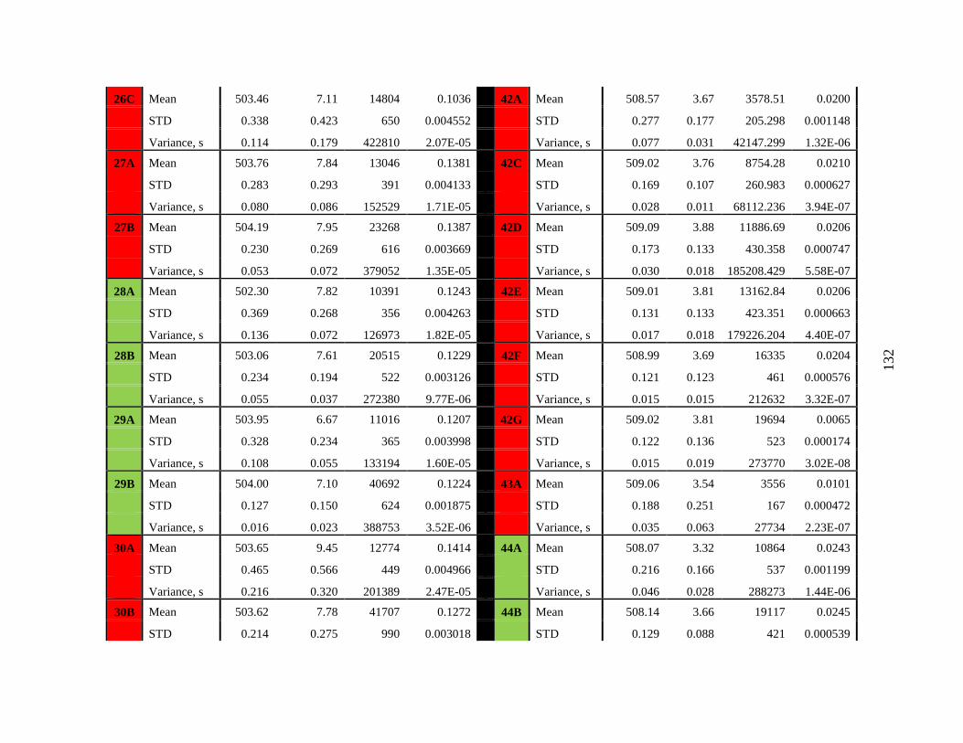
132

26C Mean 503.46 7.11 14804 0.1036 42A Mean 508.57 3.67 3578.51 0.0200

STD 0.338 0.423 650 0.004552 STD 0.277 0.177 205.298 0.001148


27A Mean 503.76 7.84 13046 0.1381 42C Mean 509.02 3.76 8754.28 0.0210

STD 0.283 0.293 391 0.004133 STD 0.169 0.107 260.983 0.000627


27B Mean 504.19 7.95 23268 0.1387 42D Mean 509.09 3.88 11886.69 0.0206

STD 0.230 0.269 616 0.003669 STD 0.173 0.133 430.358 0.000747


28A Mean 502.30 7.82 10391 0.1243 42E Mean 509.01 3.81 13162.84 0.0206

STD 0.369 0.268 356 0.004263 STD 0.131 0.133 423.351 0.000663


28B Mean 503.06 7.61 20515 0.1229 42F Mean 508.99 3.69 16335 0.0204

STD 0.234 0.194 522 0.003126 STD 0.121 0.123 461 0.000576

Variance, s 0.055 0.037 272380 9.77E-06 Variance, s 0.015 0.015 212632 3.32E-07

29A Mean 503.95 6.67 11016 0.1207 42G Mean 509.02 3.81 19694 0.0065

STD 0.328 0.234 365 0.003998 STD 0.122 0.136 523 0.000174


29B Mean 504.00 7.10 40692 0.1224 43A Mean 509.06 3.54 3556 0.0101

STD 0.127 0.150 624 0.001875 STD 0.188 0.251 167 0.000472


30A Mean 503.65 9.45 12774 0.1414 44A Mean 508.07 3.32 10864 0.0243

STD 0.465 0.566 449 0.004966 STD 0.216 0.166 537 0.001199


30B Mean 503.62 7.78 41707 0.1272 44B Mean 508.14 3.66 19117 0.0245

STD 0.214 0.275 990 0.003018 STD 0.129 0.088 421 0.000539

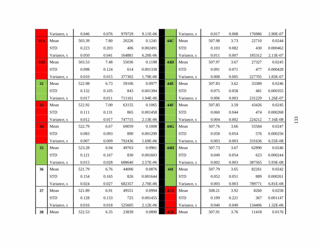
133


31A Mean 503.39 7.80 20226 0.1241 44C Mean 507.98 3.73 22710 0.0244

STD 0.223 0.203 406 0.002491 STD 0.103 0.082 430 0.000462


31B Mean 503.53 7.48 55036 0.1198 44D Mean 507.97 3.67 27327 0.0245

STD 0.098 0.124 614 0.001338 STD 0.091 0.071 477 0.000428


32 Mean 522.98 6.73 59106 0.0977 44E Mean 507.83 3.62 33389 0.0246

STD 0.132 0.105 843 0.001394 STD 0.075 0.058 481 0.000355


33 Mean 522.92 7.00 63155 0.1065 44F Mean 507.85 3.59 43426 0.0245

STD 0.111 0.131 865 0.001458 STD 0.060 0.044 474 0.000268


34 Mean 522.79 6.67 69059 0.1008 44G Mean 507.76 3.66 55584 0.0247

STD 0.083 0.093 890 0.001299 STD 0.058 0.054 576 0.000256


35 Mean 523.28 6.94 49763 0.0961 44H Mean 507.73 3.67 62890 0.0246

STD 0.121 0.167 830 0.001603 STD 0.049 0.054 623 0.000244


36 Mean 521.79 6.76 44006 0.0876 44I Mean 507.79 3.65 82261 0.0242

STD 0.154 0.165 826 0.001644 STD 0.052 0.051 889 0.000261


37 Mean 521.89 6.91 49551 0.0994 45A Mean 508.21 3.92 8260 0.0258

STD 0.128 0.133 725 0.001455 STD 0.199 0.221 367 0.001147


38 Mean 522.53 6.35 23839 0.0890 45B Mean 507.91 3.76 11418 0.0176

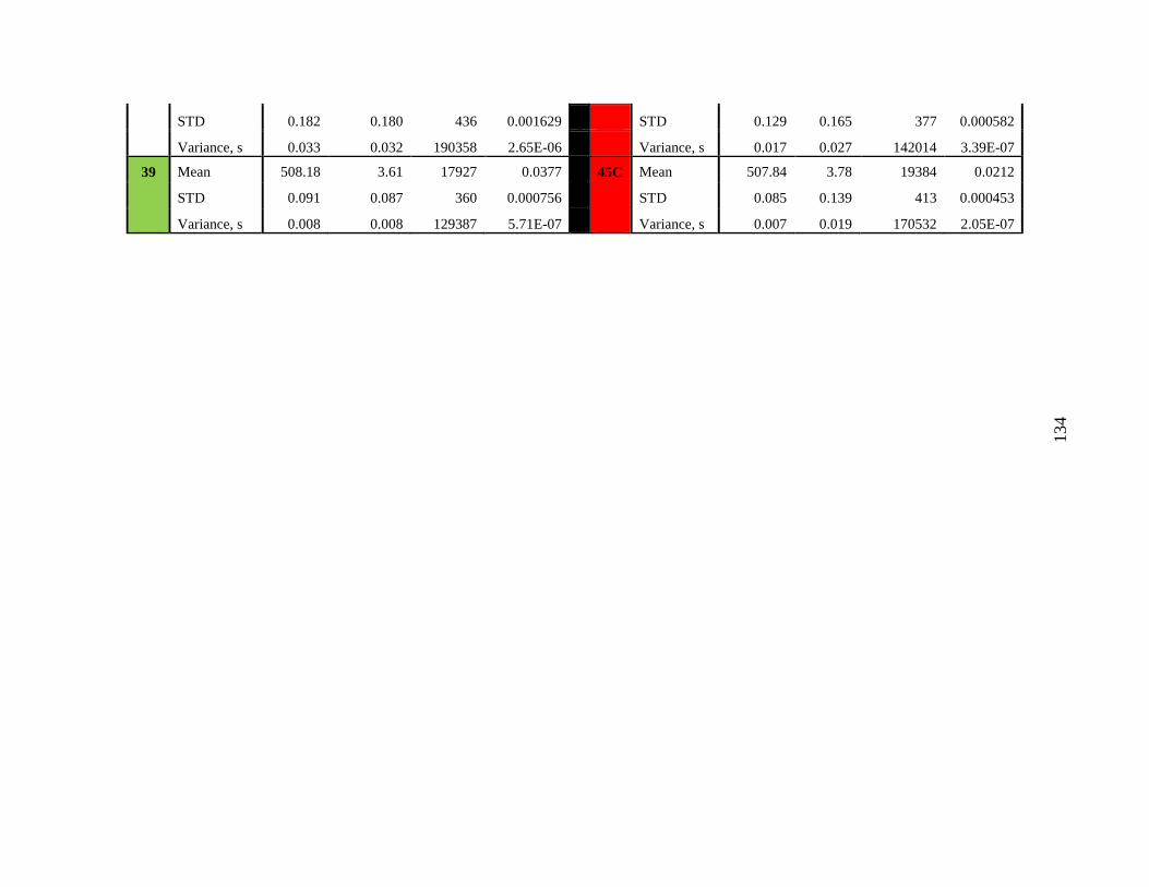
134

STD 0.182 0.180 436 0.001629 STD 0.129 0.165 377 0.000582


39 Mean 508.18 3.61 17927 0.0377 45C Mean 507.84 3.78 19384 0.0212

STD 0.091 0.087 360 0.000756 STD 0.085 0.139 413 0.000453


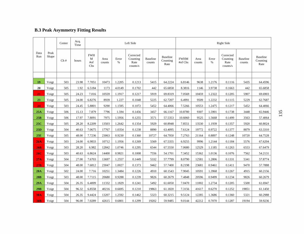
135

B.3 Peak Asymmetry Fitting Results

Data Run

Peak Shape

Center Acq.

Time Left Side Right Side

Ch # hours

FWH

M #of

Chs

Area counts

Error %

Corrected

Counting Rate

counts/s

Baseline counts

Baseline

Counting

Rate

FWHM #of Chs

Area counts

Error %

Corrected

Counting Rate

counts/s

Baseline counts

Baseline

Counting

Rate

19 Voigt 503 23.98 7.7051 10473 1.2205 0.1213 5415 64.2224 6.8146 9638 1.2176 0.1116 5435 64.4596

20 Voigt 505 1.92 6.5184 1173 4.0149 0.1702 442 65.6858 8.3816 1146 3.9738 0.1663 442 65.6858

21 Voigt 505 24.23 7.016 10559 1.1917 0.1217 5919 69.8319 7.0569 10459 1.2322 0.1205 5907 69.6903

23 Voigt 505 24.00 6.8276 8939 1.227 0.1048 5225 62.7207 6.4991 9509 1.2232 0.1115 5229 62.7687

24 Voigt 503 24.45 5.8801 9290 1.1595 0.1072 5452 64.4066 7.5266 10553 1.2475 0.1217 5452 64.4066

25A Voigt 506 15.13 7.879 7796 1.594 0.1456 3457 66.1167 10.8780 9307 1.5901 0.1738 3448 65.9446

25B Voigt 506 17.97 7.8091 7975 1.5956 0.1255 3571 57.5353 10.6060 9525 1.5668 0.1499 3563 57.4064

25C Voigt 505 28.20 8.2209 13503 1.2642 0.1354 5929 60.8948 7.8551 13530 1.1939 0.1357 5920 60.8024

25D Voigt 504 40.63 7.0675 17767 1.0354 0.1238 8890 63.4095 7.6124 19772 0.9722 0.1377 8879 63.3310

25E Voigt 505 48.00 7.7236 23063 0.9230 0.1360 10727 64.7950 7.2763 21164 0.8897 0.1248 10720 64.7528

26A Voigt 503 24.00 6.9833 10712 1.1956 0.1269 5569 67.5355 6.9255 9996 1.2144 0.1184 5576 67.6204

26B Voigt 503 28.20 6.982 12842 1.0746 0.1295 6544 67.5550 7.0680 12529 1.1185 0.1263 6553 67.6479

26C Voigt 503 40.63 6.8624 14400 0.9821 0.1008 7556 54.1701 7.3452 15362 1.0136 0.1076 7562 54.2131

27A Voigt 504 27.00 7.6703 13697 1.2557 0.1449 5332 57.7799 8.0790 12581 1.2806 0.1331 5341 57.8774

27B Voigt 504 48.00 7.6812 23047 1.0027 0.1373 9462 57.7400 8.2198 23681 0.9461 0.1411 9470 57.7888

28A Voigt 502 24.00 7.716 10251 1.3484 0.1226 4910 60.1543 7.9045 10591 1.3968 0.1267 4915 60.2156

28B Voigt 503 48.00 7.7115 20680 0.9288 0.1239 9826 60.2679 7.4848 20596 0.9499 0.1234 9826 60.2679

29A Voigt 504 26.35 6.4009 11332 1.1829 0.1241 5492 61.6050 7.0470 11002 1.2734 0.1205 5500 61.6947

29B Voigt 504 96.32 6.8558 40216 0.6695 0.1210 19863 61.1820 7.3156 41617 0.6270 0.1252 19851 61.1450

30A Voigt 504 26.35 9.4424 13207 1.2592 0.1462 5323 60.3215 9.5124 12285 1.3686 0.1360 5321 60.2988

30B Voigt 504 96.00 7.0289 42615 0.6801 0.1299 19202 59.9485 9.0144 42212 0.7070 0.1287 19194 59.9236

136

31A Voigt 503 48.08 7.2214 19252 0.9845 0.1181 8794 55.2357 8.3330 21309 1.0666 0.1307 8787 55.1917

31B Voigt 504 136.08 7.5511 57747 0.5930 0.1257 24570 54.7846 7.4659 53063 0.5963 0.1155 24573 54.7913

32 Voigt 523 182.47 6.8311 60009 0.5657 0.0992 29313 49.6193 6.6495 59014 0.6548 0.0976 29321 49.6329

33 Voigt 523 182.53 6.6956 63799 0.5324 0.1076 30441 52.5718 7.3747 63740 0.5414 0.1075 30464 52.6116

34 Voigt 523 217.42 6.6126 71190 0.4868 0.1039 35265 52.6837 6.7452 67952 0.4994 0.0991 35287 52.7165

35 Voigt 523 167.53 7.243 50066 0.6243 0.0967 22857 45.2231 6.7813 50721 0.6471 0.0980 22874 45.2567

36 Voigt 522 165.52 7.1609 45078 0.6451 0.0897 20786 42.3719 6.3394 43520 0.7473 0.0866 20764 42.3270

37 Voigt 522 167.17 6.8121 50488 0.5940 0.1013 24961 51.2923 7.0286 49515 0.6030 0.0994 24962 51.2943

38 Voigt 523 91.08 6.5012 25027 0.9455 0.0935 11242 42.9875 6.2743 23045 0.8992 0.0861 11241 42.9836

39 Voigt 508 164.17 3.5287 17573 0.8484 0.0369 14636 31.4914 3.6958 19231 0.7858 0.0404 14625 31.4677

40A Voigt 508 122.17 3.5033 7524 1.0764 0.0229 6562 20.4882 4.1130 8768 1.0730 0.0267 6558 20.4757

40B Voigt 509 239.58 3.9037 16732 0.8176 0.0262 12406 19.8749 3.5711 15412 0.7784 0.0241 12401 19.8669

40C Voigt 509 293.33 3.919 20120 0.7607 0.0258 14947 19.6138 3.7130 19226 0.7117 0.0246 14947 19.6138

40D Voigt 509 410.83 3.9592 28001 0.6456 0.0258 19918 18.7785 3.7252 26533 0.6370 0.0244 19917 18.7776

40E Voigt 509 433.58 3.9219 28760 0.6345 0.0251 20756 18.5642 3.7625 27718 0.6352 0.0242 20754 18.5624

40F Voigt 509 510.92 3.9119 33739 0.5953 0.0251 24022 18.3084 3.7332 32395 0.5983 0.0241 24015 18.3030

41A Voigt 509 116.58 3.6042 6947 1.3186 0.0234 4280 14.7692 3.4659 6568 1.3287 0.0221 4280 14.7692

41B Voigt 509 167.50 3.7684 10293 1.0862 0.0242 6273 15.1073 3.4129 9117 1.1218 0.0214 6273 15.1073

41C Voigt 509 237.50 3.5388 14217 0.9220 0.0237 9135 15.5735 3.1949 13025 0.9288 0.0217 9131 15.5666

41D Voigt 509 283.17 3.5633 16901 0.8418 0.0237 10879 15.5934 3.2255 15274 0.8629 0.0214 10873 15.5848

41E Voigt 509 332.75 3.6781 20317 0.7773 0.0243 12852 15.7178 3.3994 18430 0.7941 0.0220 12847 15.7117

41F Voigt 509 497.75 3.7208 28483 0.6722 0.0229 17688 14.5886 3.5516 26029 0.6885 0.0210 17690 14.5902

42A Voigt 509 73.93 4.0944 3962 1.791 0.0222 2178 12.4751 3.2158 3375 1.9352 0.0189 2177 12.4693

42C Voigt 509 172.95 3.7745 8765 1.1952 0.0211 5444 13.4001 3.7432 9153 1.6902 0.0220 5437 13.3829

42D Voigt 509 240.38 3.7238 11757 1.031 0.0204 7097 12.6135 4.0458 12606 1.3946 0.0219 7089 12.5993

42E Voigt 509 266.75 3.7087 13212 0.979 0.0207 7707 12.3611 3.9423 13684 1.3146 0.0214 7700 12.3498

42F Voigt 509 335.80 3.6408 16574 0.8980 0.0207 9627 12.3106 3.7749 16849 1.1233 0.0210 9621 12.3029

42G Voigt 509 1331.05 3.7131 19864 0.8368 0.0066 11663 3.9669 3.9328 20395 0.9837 0.0068 11654 3.9638

43A Voigt 509 168.33 2.9351 3569 1.6707 0.0101 2797 8.1159 4.2225 3767 1.7894 0.0107 2796 8.1130

44A Voigt 508 218.08 3.3525 10925 0.9748 0.0244 8942 20.4421 3.3302 11517 0.9388 0.0257 8939 20.4353

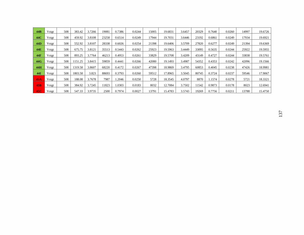
137

44B Voigt 508 383.42 3.7266 19081 0.7386 0.0244 15005 19.6831 3.6457 20329 0.7640 0.0260 14997 19.6726

44C Voigt 508 459.92 3.8108 23258 0.6514 0.0249 17944 19.7031 3.6446 23192 0.6861 0.0249 17934 19.6921

44D Voigt 508 552.92 3.8107 28338 0.6026 0.0254 21398 19.6406 3.5709 27820 0.6277 0.0249 21394 19.6369

44E Voigt 508 675.75 3.8121 35513 0.5443 0.0262 25923 19.5963 3.4449 33095 0.5635 0.0244 25922 19.5955

44F Voigt 508 893.25 3.7764 46213 0.4953 0.0261 33829 19.5708 3.4209 43149 0.4727 0.0244 33838 19.5761

44G Voigt 508 1151.25 3.8415 59859 0.4441 0.0266 42080 19.1493 3.4987 54352 0.4353 0.0242 42096 19.1566

44H Voigt 508 1319.58 3.8607 68220 0.4172 0.0267 47398 18.9869 3.4795 60853 0.4045 0.0238 47426 18.9981

44I Voigt 508 1803.58 3.823 88693 0.3793 0.0260 59512 17.8965 3.5045 80745 0.3724 0.0237 59546 17.9067

45A Voigt 508 188.08 3.7678 7987 1.2046 0.0250 5728 18.3545 4.0797 8870 1.1574 0.0278 5721 18.3321

45B Voigt 508 384.92 3.7245 11823 1.0303 0.0183 8032 12.7084 3.7502 11542 0.9873 0.0178 8023 12.6941

45C Voigt 508 547.33 3.9735 2500 0.7974 0.0027 13791 15.4783 3.5743 19269 0.7756 0.0211 13788 15.4750

138

Bibliography

1. Chen, YL, Yang, DP. Mössbauer Effect in Lattice Dynamics. Wiley-VCH: KGaA,

Weinham, 2007.

2. Cranshaw, TE, Dale BW, Longworth GO and Johnson CE. Mössbauer

Spectroscopy and its Applications. Cambridge Univ. Press: Cambridge, 1985.

3. Cranshaw, T.E., Schiffer, J. P., Measurement of the gravitational red shift with

the Mössbauer effect. Proc. Physic. Soc. 84 245pp, 1964.

4. DeGrave E, Vandenberghe RE, Dauwe C. ILEEMS: Methodology and

applications to iron oxides. Hyperfine Interactions, 161 (1-4): 147-160, 2005.

5. Dickson DPE and Berry FJ. Mössbauer Spectroscopy. Cambridge Univ. Press:

Cambridge, 1986.

6. Dyar, MD, Agresti, DG, Schaefer, M, Grant, CA, and Sklute, EC. “Mössbauer

spectroscopy of earth and planetary materials.” Annual Reviews of Earth and

Planetary Science, 34, 83-125, 2006.

7. Frauenfelder, H. The Mössbauer Effect. Benjamin: New York, 1962.

8. Fultz, B. “Mössbauer Spectroscopy,” in Characterization of Materials. Kaufmann,

Editor. John Wiley: New York, 2011.

9. Jones, W., Thomas, J.M., Thorpe, R.K., Tricker, M.J. “Conversion Electron

Mössbauer Spectroscopy and the Study of Surface Properties and Reactions”,

Applications of Surface Science pg. 388-407., North-Holland Publishing

Company (1978)

10. Kankeleit, E. Feedback in electromechanical drive systems. In Mössbauer Effect

Methodology, vol. 1. Plenum Press, New York. (1965)

11. Knoll, G. E., Radiation Detection and Measurement, John Wiley & Sons, New

York, NY, USA, 3rd edition, 2000

12. Krane, K. S. Introductory Nuclear Physics. Oregon State University: John Wiley

& Sons, 1988.

13. Lang, G., (1970) "Mössbauer Spectroscopy of Haem Proteins", Quart. Rev.

Biophysics 3, I 1-60.

14. Lang, G. and Marshall, W. (1966) "Mössbauer Effect in Some Hemoglobin

Compounds", Proc. Phys. Soc. 87, 3-34.

139

15. Long, GJ and Grandjean, F, eds. Mössbauer Spectroscopy Applied to Magnetism

and Materials Science Vol. 1. Plenum: New York, 1993.

16. Long, G. J. and Stevens, J. G., eds. (1986) "Industrial applications of the

Mössbauer Effect", Plenum Press, New York.

17. May L, ed. An Introduction toMössbauer Spectroscopy. New York: Plenum.

203pp, 1971.

18. McKelvey, J., Solid State Physics for Engineering and Material Science, Krieger

Publishing Co. 1st ed. (2003)

19. Mössbauer, R. L. Kernresonanzfluoreszenz von Gamma-strahlung in Ir191

. Z.

Phys. 151:124, 1958.

20. O’Haver, T., Pragmatic Introduction to Signal Processing with applications in

chemical analysis. University of Maryland, 16 Mar 2014.

21. Seberini, M. and Sitek, J. Surface Analysis of Iron – Containing Samples by

CEMS an Overview of the Method. Journal of Electrical Engineering, Vol 59,

No 5: pg 234-240 (2008)

22. Seitz, F. and Koehler, J. S., in Solid State Physics, edited by H. Ehrenreich, F.

Seitz, and D. Turnbull (Academic, New York, 1956), Vol. 2, p. 351

23. Spikerman, J.J. Conversion Electron Mössbauer Spectroscopy. In Mössbauer

Effect Methodology, vol. 7. Plenum Press, New York. (1971)

24. Spikerman, J.J. Mossbauer Spectroscopy Instruction Manual for the MS-1200.

Ranger Scientific, Inc., Burleson, TX.

25. Stewart, I., Tricker, M. J., Cairns, J. A. “Mössbauer Spectroscopic Studies of

Chromium Depletion in a 310 Stainless Steel During Air Oxidation”, Corrosion

Science Vol 26., Pergamon Journals Ltd, Great Britain (1986)

26. Tanis, E.A., Partial phonon densitiy of states of 57-iron and 161-dysprosium in

DyFe3 by nuclear resonant inelastic X-ray scattering under high pressure. MS

Thesis. University of Nevada, Las Vegas. (2006)

27. Thompson, B., Exploring the Replicability of a Study’s results: Bootstrap

Statistics for the Multivariate Case. Texas A&M University Sage Journals. (2012)

28. Vandenberghe R.E., DeGrave E., Dauwe C. ILEEMS: On the methodology of

Mossbauer spectra. Hyperfine Interactions 83: pg 29-49, 1994.

29. Wegener H. 1965. Der M¨ossbauer-Effekt und Seine Anwendung in Physik und

Chemie. Mannheim: Bibliogr. Institut. 214pp.

140

30. Wit, H.P., Hoeksema, G., Niesen, L. and de Waard, H. A multi-purpose velocity

transducer for Mössbauer spectrometers. Nuclear Instrument Methods, vol 141

(1977)

REPORT DOCUMENTATION PAGE Form Approved OMB No. 074-0188

The public reporting burden for this collection of information is estimated to average 1 hour per response, including the time for reviewing instructions, searching existing data sources, gathering and maintaining the data needed, and completing and reviewing the collection of information. Send comments regarding this burden estimate or any other aspect of the collection of information, including suggestions for reducing this burden to Department of Defense, Washington Headquarters Services, Directorate for Information Operations and Reports (0704-0188), 1215 Jefferson Davis Highway, Suite 1204, Arlington, VA 22202-4302. Respondents should be aware that notwithstanding any other provision of law, no person shall be subject to any penalty for failing to comply with a collection of information if it does not display a currently valid OMB control number.

PLEASE DO NOT RETURN YOUR FORM TO THE ABOVE ADDRESS.

1. REPORT DATE (DD-MM-YYYY)

04-03-2015 2. REPORT TYPE

Master’s Thesis 3. DATES COVERED (From – To)

20 Aug 2010 – 22 Jan 2015

4. TITLE AND SUBTITLE

Coupling Nuclear Induced Phonon Propagation with Conversion

Electron Mössbauer Spectroscopy

5a. CONTRACT NUMBER

5b. GRANT NUMBER

5c. PROGRAM ELEMENT NUMBER

6. AUTHOR(S)

Parker, Michael J., Captain, USAF

5d. PROJECT NUMBER

N/A 5e. TASK NUMBER

5f. WORK UNIT NUMBER

7. PERFORMING ORGANIZATION NAMES(S) AND ADDRESS(S)

Air Force Institute of Technology

Graduate School of Engineering and Management (AFIT/EN)

2950 Hobson Way, Building 640

WPAFB OH 45433-8865

8. PERFORMING ORGANIZATION REPORT NUMBER


9. SPONSORING/MONITORING AGENCY NAME(S) AND ADDRESS(ES)

Department of Homeland Security – Domestic Nuclear Detection Office

245 Murray Dr, Building 410 Washington, DC 20528

Attn: DNDO Email: [email protected]

10. SPONSOR/MONITOR’S ACRONYM(S)

DHS/DNDO

11. SPONSOR/MONITOR’S REPORT NUMBER(S)

12. DISTRIBUTION/AVAILABILITY STATEMENT

DISTIBUTION STATEMENT A. APPROVED FOR PUBLIC RELEASE; DISTRIBUTION UNLIMITED.

13. SUPPLEMENTARY NOTES

This material is declared a work of the U.S. Government and is not subject to copyright protection in the United States.

14. ABSTRACT

Mössbauer spectroscopy is a very sensitive measurement technique (~10-8 eV) which prompted motivation for the experiment

described in this thesis. Namely, can a sensitive detection system be developed to detect nuclear recoils on the order of 10 to 100 of

eVs? The hypothesis that this thesis tests is: Nuclear induced phonon bursts caused by Rutherford scattered alphas, decayed from

241Am, in a type-310 stainless steel material can couple with 7.3keV conversion electron Mössbauer events at the other end of the

material which will have a statistically significant effect on a Mössbauer spectrum. The phonon bursts produced by the alpha

collisions are expected to be very low energy at the other end of length of material. Since Mössbauer spectroscopy is sensitive and

can detect the very low energy phonons, the spectrum is expected to change in at least one of the five areas after coupling occurs:

broadening in the spectrum peaks, increased/decreased background counting rate, Mössbauer peak asymmetry,

increased/decreased counting rate under the peak, and/or a peak centroid shift. This research aims to determine the significance of

changes between spectra with phonon bursts and with no phonon bursts through hypothesis testing, where the null hypothesis is

where phonons do not affect Mössbauer spectra in one of the five areas mentioned previously. After the spectra and results were

analyze using an f-test and t-test comparisons, this experiment failed to reject the null result. Leading to the conclusion that

additional research must be conducted. 15. SUBJECT TERMS

Mössbauer Spectroscopy, Detection, Phonons

16. SECURITY CLASSIFICATION OF: 17. LIMITATION OF ABSTRACT

U

18. NUMBER OF PAGES

154

19a. NAME OF RESPONSIBLE PERSON

Dr. Larry Burggraf a. REPORT

U

b. ABSTRACT

U

c. THIS PAGE

U

19b. TELEPHONE NUMBER (Include area code)

(937) 255-3636, x 4507

([email protected]) Standard Form 298 (Rev. 8-98)

Prescribed by ANSI Std. Z39-18

Documents

COUPLING NUCLEAR INDUCED PHONON … · coupling nuclear induced phonon propagation with conversion electron mÖssbauer spectroscopy thesis michael j. parker, capt, usaf afit-enp-ms-15-j-054