Working Papers

304

ISSN 1518-3548

Jaqueline Terra Moura Marins and Myrian Beatriz Eiras das Neves

Credit Default and Business Cycles:

an investigation of this relationship in

the Brazilian corporate credit market

March, 2013

ISSN 1518-3548 CNPJ 00.038.166/0001-05

Working Paper Series Brasília n. 304 Mar. 2013 p. 1-32

Working Paper Series Edited by Research Department (Depep) – E-mail: workingpaper@bcb.gov.br Editor: Benjamin Miranda Tabak – E-mail: benjamin.tabak@bcb.gov.br Editorial Assistant: Jane Sofia Moita – E-mail: jane.sofia@bcb.gov.br Head of Research Department: Eduardo José Araújo Lima – E-mail: eduardo.lima@bcb.gov.br The Banco Central do Brasil Working Papers are all evaluated in double blind referee process. Reproduction is permitted only if source is stated as follows: Working Paper n. 304. Authorized by Carlos Hamilton Vasconcelos Araújo, Deputy Governor for Economic Policy. General Control of Publications Banco Central do Brasil

Comun/Dipiv/Coivi

SBS – Quadra 3 – Bloco B – Edifício-Sede – 14º andar

Caixa Postal 8.670

70074-900 Brasília – DF – Brazil

Phones: +55 (61) 3414-3710 and 3414-3565

Fax: +55 (61) 3414-1898

E-mail: editor@bcb.gov.br

The views expressed in this work are those of the authors and do not necessarily reflect those of the Banco Central or its members. Although these Working Papers often represent preliminary work, citation of source is required when used or reproduced. As opiniões expressas neste trabalho são exclusivamente do(s) autor(es) e não refletem, necessariamente, a visão do Banco Central do Brasil. Ainda que este artigo represente trabalho preliminar, é requerida a citação da fonte, mesmo quando reproduzido parcialmente. Citizen Service Division Banco Central do Brasil

Deati/Diate

SBS – Quadra 3 – Bloco B – Edifício-Sede – 2º subsolo

70074-900 Brasília – DF – Brazil

Toll Free: 0800 9792345

Fax: +55 (61) 3414-2553

Internet: <http//www.bcb.gov.br/?CONTACTUS>

Credit Default and Business Cycles: an

investigation of this relationship in the

Brazilian corporate credit market

Jaqueline Terra Moura Marins∗

Myrian Beatriz Eiras das Neves∗∗

Abstract

The Working Papers should not be reported as representing the

views of the Banco Central do Brasil. The views expressed in the

papers are those of the author(s) and do not necessarily reflect

those of the Banco Central.

The aim of this paper is to examine empirically whether the

default of borrower companies in the Brazilian market rises in

downturns. To this end, a probit model for the probability of

default is developed based on credit microdata taken from the

Credit Information System of the Central Bank of Brazil

(SCR) and on macroeconomic variables. Our results provide

evidence of a strong negative relationship between business

cycle and credit default, going in accord to the literature

dealing with corporate data. These effects are stronger than

those found in our previous article for the case of default of

∗ Research Department, Central Bank of Brazil. E-mail: jaqueline.terra@bcb.gov.br ∗∗ Supervision Department, Central Bank of Brazil. E-mail: myrian.neves@bcb.gov.br

3

individuals. This is an expected result, since the retail credit is

more sprayed than the corporate credit. The macroeconomic

variables that have the greatest effect on corporate defaults

were GDP growth and inflation.

Keywords: Procyclicality, Business Cycle, Corporate Credit

Risk, Basel II.

JEL Classification: G21, G28, E32.

4

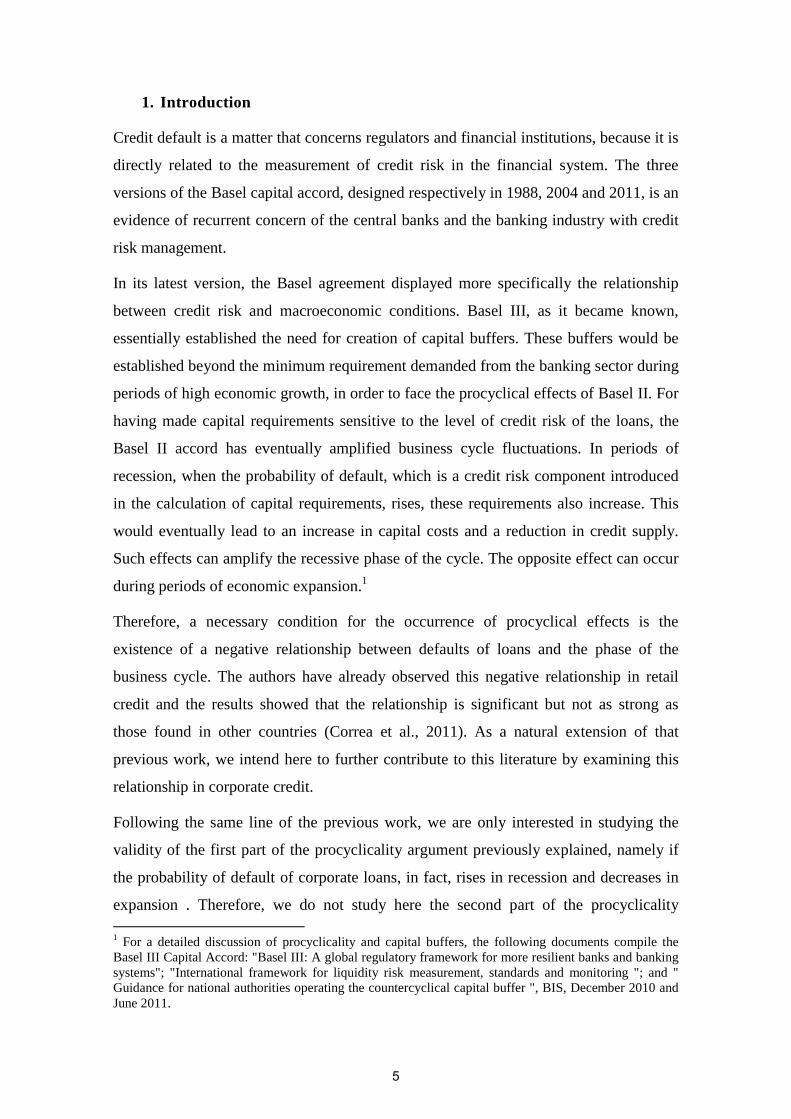
1. Introduction

Credit default is a matter that concerns regulators and financial institutions, because it is

directly related to the measurement of credit risk in the financial system. The three

versions of the Basel capital accord, designed respectively in 1988, 2004 and 2011, is an

evidence of recurrent concern of the central banks and the banking industry with credit

risk management.

In its latest version, the Basel agreement displayed more specifically the relationship

between credit risk and macroeconomic conditions. Basel III, as it became known,

essentially established the need for creation of capital buffers. These buffers would be

established beyond the minimum requirement demanded from the banking sector during

periods of high economic growth, in order to face the procyclical effects of Basel II. For

having made capital requirements sensitive to the level of credit risk of the loans, the

Basel II accord has eventually amplified business cycle fluctuations. In periods of

recession, when the probability of default, which is a credit risk component introduced

in the calculation of capital requirements, rises, these requirements also increase. This

would eventually lead to an increase in capital costs and a reduction in credit supply.

Such effects can amplify the recessive phase of the cycle. The opposite effect can occur

during periods of economic expansion.1

Therefore, a necessary condition for the occurrence of procyclical effects is the

existence of a negative relationship between defaults of loans and the phase of the

business cycle. The authors have already observed this negative relationship in retail

credit and the results showed that the relationship is significant but not as strong as

those found in other countries (Correa et al., 2011). As a natural extension of that

previous work, we intend here to further contribute to this literature by examining this

relationship in corporate credit.

Following the same line of the previous work, we are only interested in studying the

validity of the first part of the procyclicality argument previously explained, namely if

the probability of default of corporate loans, in fact, rises in recession and decreases in

expansion . Therefore, we do not study here the second part of the procyclicality 1 For a detailed discussion of procyclicality and capital buffers, the following documents compile the Basel III Capital Accord: "Basel III: A global regulatory framework for more resilient banks and banking systems"; "International framework for liquidity risk measurement, standards and monitoring "; and " Guidance for national authorities operating the countercyclical capital buffer ", BIS, December 2010 and June 2011.

5

argument, i.e., if the increase in the probability of default, while resulting in a higher

capital requirement, will be reflected in a reduction of credit supply. That would require

a separation of the effects of supply and demand for credit, which is not possible given

the information we have.

In this context, the aim of this paper is to examine empirically whether the default of

borrower companies in the Brazilian market rises in downturns. To this end, a probit

model for the probability of default is developed based on credit microdata taken from

the Credit Information System of the Central Bank of Brazil (SCR) and on

macroeconomic variables. In the literature of credit risk, it is common to call this type

of modeling as idiosyncratic and systemic risk factor model, respectively.

Unlike previous work, we did not select any specific type of credit modality neither

financial institution, working with the whole range of available transactions. This

resulted in a large and unprecedented microdata base for the Brazilian market of

corporate loans, which included information about more than 100,000 borrowing

companies and nearly 800 lending financial institutions between 2005 and 2010.

Our results provide evidence of a strong negative relationship between business cycle

and credit default, going according to the literature dealing with corporate data. These

effects are stronger than those found in the previous article for the case of default of

individuals. This is an expected result, since the retail credit is more sprayed than the

corporate credit. The macroeconomic variables that have the greatest effect on corporate

defaults were GDP growth and inflation.

The rest of the article is organized as follows. In Section 2, we review the literature on

the relationship between corporate default and macroeconomic variables. In section 3,

we seek evidence of this relationship, based on the observed correlations between the

time series of these variables. In section 4, we describe the set of credit microdata and

present some descriptive statistics of the sample. In section 5, the econometric model

used to investigate the relationship is presented along with the inclusion of those

microdata and, in section 6, we discuss the main results. In Section 7, some conclusions

are presented.

6

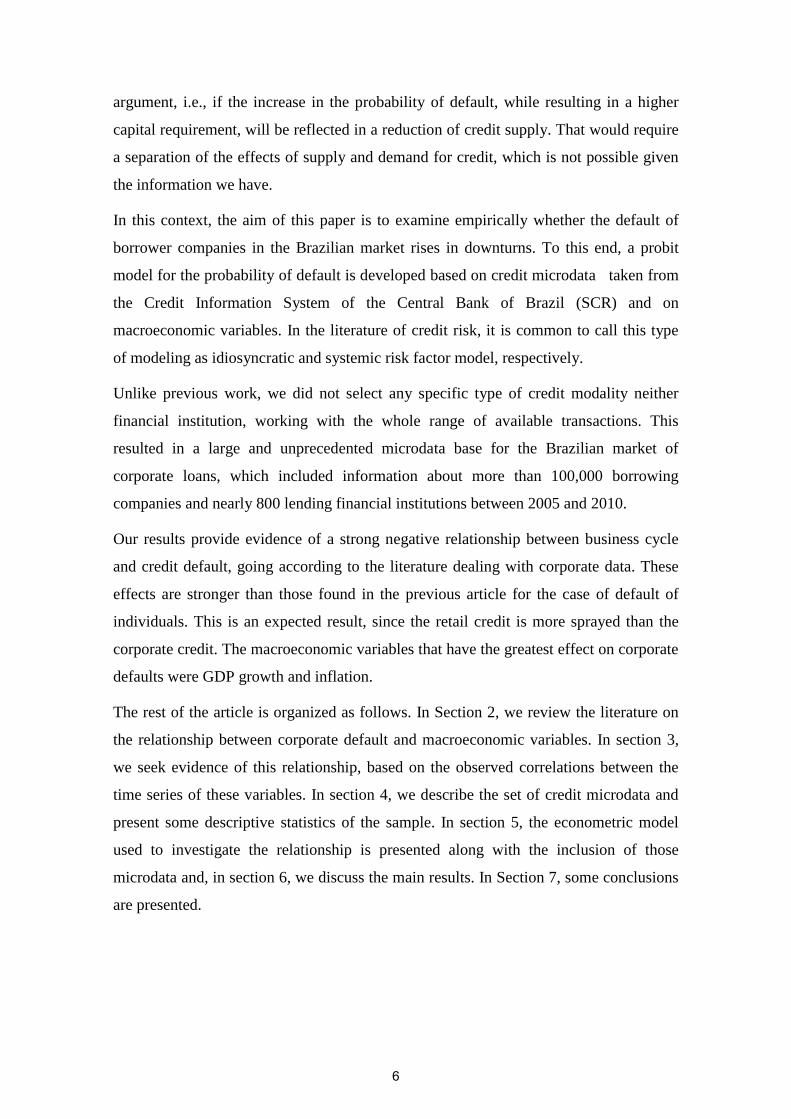
2. Literature review

The literature on the relationship between credit default and macroeconomic conditions

is still scarce. However, with the recent economic events, especially the 2008 financial

crisis, studies about macro-finance interaction became more frequent.

Some recent articles associate firm-specific financial indexes with variables related to

business cycle, when it comes to specification of default risk models. The financial

variables are related to liquidity, profitability, efficiency, solvency, leverage and firm

size.

Bharath and Shumway (2008) observed that the widely used structure of the Merton’s

model (1974) to forecast default probabilities, solely based on information from the

companies’ market value, is not enough. Works such as Duffie, Saita and Wang (2007),

Pesaran, Schuermann, Treutler and Weiner (2006), Bonfim (2009), Lando and Nielsen

(2010) and Tang and Yan (2010) present empirical evidence that firm-specific factors

alone are not able to fully explain variations in corporate defaults and credit ratings.

Bonfim (2009) examined the determinants of corporate loans defaults in the Portuguese

banking sector, through probit models and survival analysis. Using microdata, the

author found that the companies’ defaults are strongly affected by their specific

characteristics, such as its capital structure, company size, profitability and liquidity,

plus its recent sales performance and its investment policy. However, the introduction

of macroeconomic variables substantially improved the quality of the models, especially

the GDP growth rate, the lending growth rate, the average interest rate of the loans and

the stock market return rate.

According to Jacobson, Lindé and Roszbach (2011), the two most important

macroeconomic factors that affect corporate defaults are the nominal interest rate and

the output gap. As financial firm-specific variables, the authors used the EBITDA and

total assets ratio, the interest coverage index, the leverage index, the total liabilities and

revenues ratio, the net assets and total liabilities ratio and finally the turning stock.

Repullo, Saurina and Trucharte (2009) investigated the possible procyclical effects of

Basel II in the Spanish financial system between 1987 and 2008. The authors set out to

develop a logit model for the probability of default based on credit microdata related to

the loan transactions’ characteristics, the borrowing firm's characteristics and some

macroeconomic variables. The estimated probabilities of default for each company were

7

used to calculate the corresponding capital requirements of Basel II that would have

been required if the agreement were on at that time. From this rebuilt capital

requirement series, the procyclicality was verified by the presence of strong negative

correlation with the GDP growth rate. This methodology used to investigate the

procyclical effects, however, is subject to the Lucas’ critique, as the authors warned.

3. Aggregate evidence of the relationship between corporate credit default

and business cycle

Before studying the evidence of the relationship between default and macroeconomic

fluctuations in the level of credit microdata, we should try to understand some aspects

of this relationship at an aggregate level. To this end, we examined the correlation

between a series of corporate credit default with some macroeconomic variables. These

correlations will help us to better understand the cyclical movement between the

defaults and the set of macro variables considered here and therefore to identify how

these variables can be used in the probit regression model, together with microdata.

The corporate default series used here refers to the balance of principal and / or interest

installments of loans more than 90 days overdue2 .The macroeconomic series gather

information regarding the level of domestic production and the granting of credit.

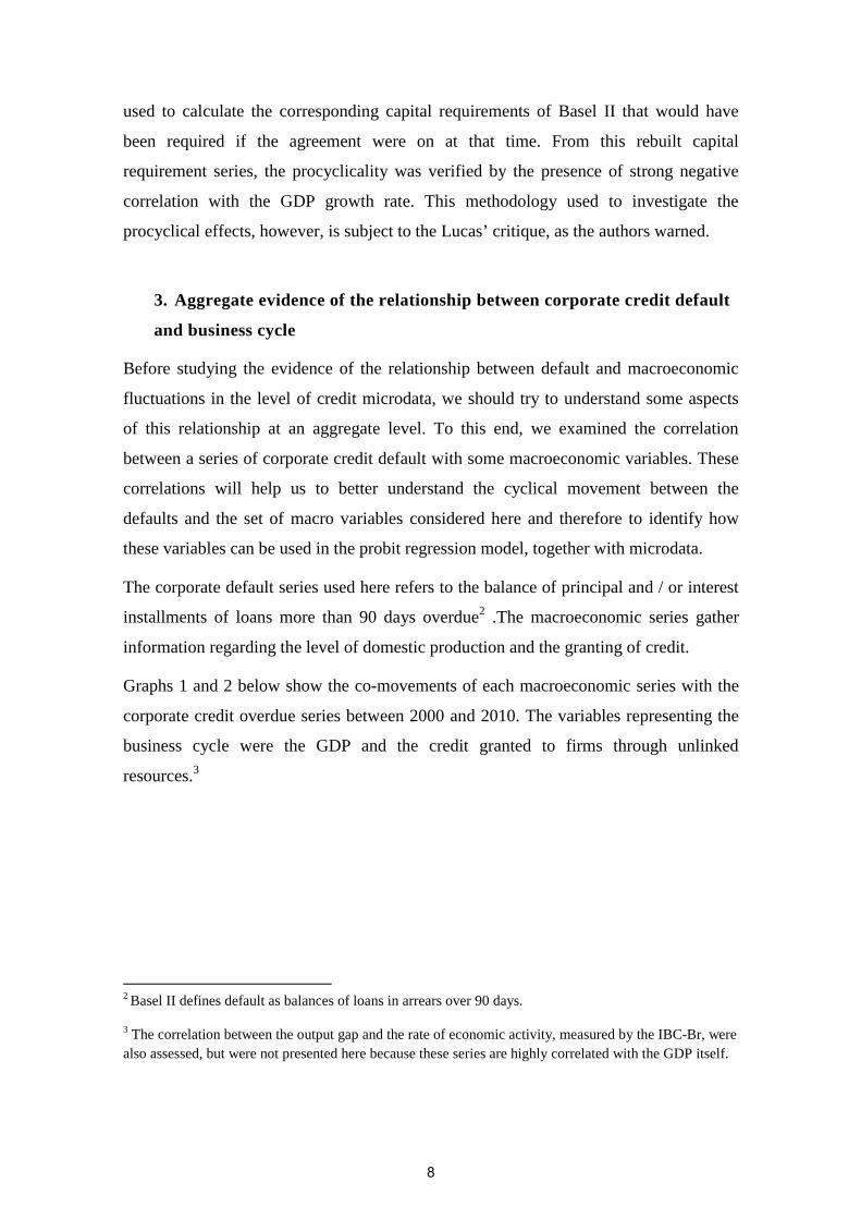
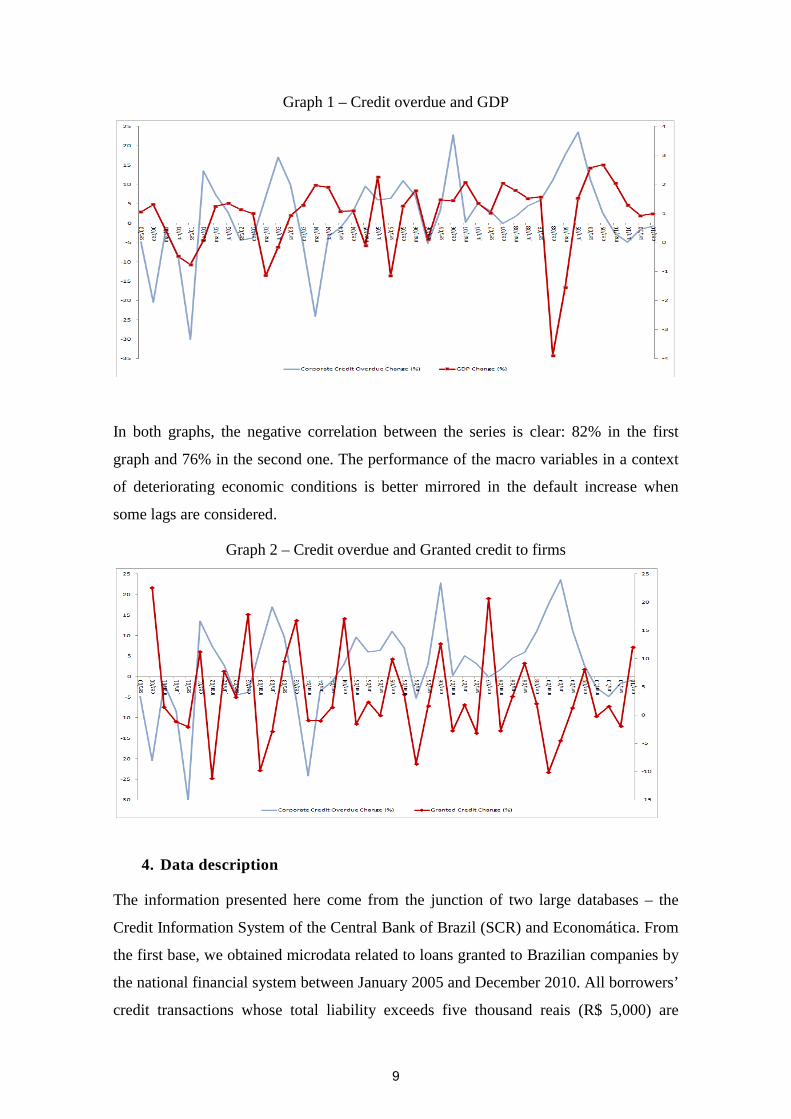
Graphs 1 and 2 below show the co-movements of each macroeconomic series with the

corporate credit overdue series between 2000 and 2010. The variables representing the

business cycle were the GDP and the credit granted to firms through unlinked

resources.3

2 Basel II defines default as balances of loans in arrears over 90 days.

3 The correlation between the output gap and the rate of economic activity, measured by the IBC-Br, were also assessed, but were not presented here because these series are highly correlated with the GDP itself.

8

Graph 1 – Credit overdue and GDP

In both graphs, the negative correlation between the series is clear: 82% in the first

graph and 76% in the second one. The performance of the macro variables in a context

of deteriorating economic conditions is better mirrored in the default increase when

some lags are considered.

Graph 2 – Credit overdue and Granted credit to firms

4. Data description

The information presented here come from the junction of two large databases – the

Credit Information System of the Central Bank of Brazil (SCR) and Economática. From

the first base, we obtained microdata related to loans granted to Brazilian companies by

the national financial system between January 2005 and December 2010. All borrowers’

credit transactions whose total liability exceeds five thousand reais (R$ 5,000) are

9

recorded in the SCR, according to the information provided by the lenders themselves

to the Central Bank of Brazil. Data are reported monthly and contain detailed

information on loans, including some characteristics of the borrowers and the

transactions, such as their risk ratings. The level of detail present in this database allows

us to analyze the components of the borrowers’ credit risk taking into account the

heterogeneity that exist among them.

The chosen sample consists on fixed-income loans granted to firms. The observation

unit combines all the transactions of each customer in a given financial institution,

regardless of their credit modality. Loans with interest rates above 250% per year were

eliminated because they could represent incorrect input on the system. After this

filtering, the resulting credit modalities were: overdraft, working capital loans with

maturities superior than 30 days, bill discount, check cashing and revolving credit. As

the remaining observations were not manageable yet (7 million), a new selection

became necessary. This time, we randomly selected and stratified by the economic

sector of the borrower, a sample of 30% of these observations. This resulted in 61,232

borrowings companies taking credit in 640 financial institutions, amounting 91,530

“financial institution / company” units.

Jarrow and Turnbull (2000) noted that one year is the time horizon used in literature to

measure credit risk issues. Despite the wealth of information present in the SCR, we

considered time intervals of less than one year, like quarters, due to the small number of

years available in our database (2005 to 2010).

A defaulting firm on a given institution was the one which has credit loans overdue for

over 90 days. According to this, the same firm can be considered not in default in

another financial institution.

Regarding the characteristics of the borrower, the SCR provides information on its size

(micro, small, medium or large company), its type of control (public or private), the

main economic sector of its activity (according to the CNAE’s code of IBGE) and the

geographic region of the credit granting agency. From this data, we constructed

variables to represent the number of financial institutions with which the company has a

credit relationship, the percentage of the company’s portfolio that is collateralized, the

portfolio´s average interest rate and the company’s average total debt in the National

Financial System.

10

We extracted financial information from Economática, the second database used in this

article. As customers are not identified in the SCR for reasons of confidentiality, we

could not cross the data on loans with the balance sheet data of the borrowing firm.

Thus, we used sector variables extracted from the Economática related to liquidity,

profitability, efficiency, solvency and leverage. We selected the following variables:

return on equity, earnings to price ratio, earnings per share, liabilities to assets, total

assets, EBITDA margin, nominal cost of debt, net debt to EBITDA ratio, liquidity ratio,

financial leverage, financial cycle, index risk and Sharpe ratio4. Each sector variable

was represented by its median value on a quarter and was equally allocated to all

companies of the same sector in that quarter.5

4.1. Descriptive statistics

Based on the sample used here, Table 1 shows the total number of companies in each

sector, the value of the loan portfolio in December 2010 and the average default rate.

Construction is the highest default rate sector (5.3%), also with the largest loan portfolio

(US$ 15 billion). Moreover, Electricity is the sector with the lowest level of delay

(0.9%) and Telecommunications has the lowest loan portfolio (US$ 92 million).

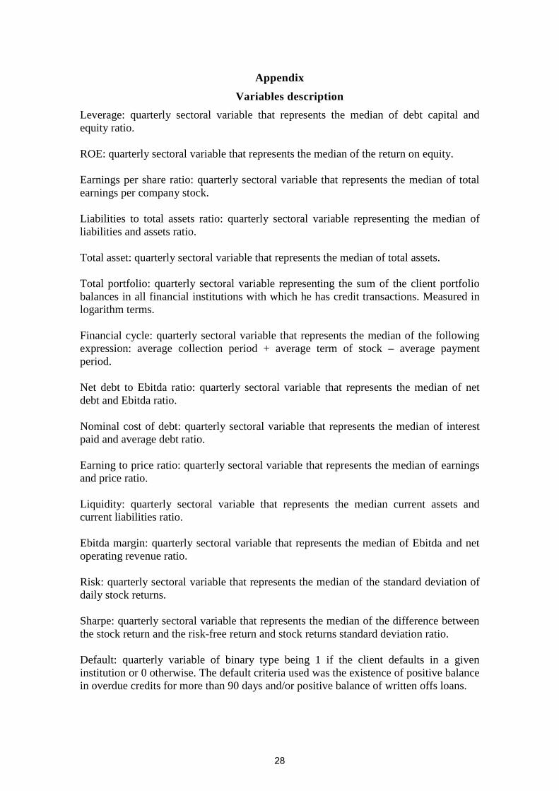
4 These variables are described in the Appendix.

5 We redistributed the 24 CNAE’s macro-sectors into the 19 Economática’s sectors.

11

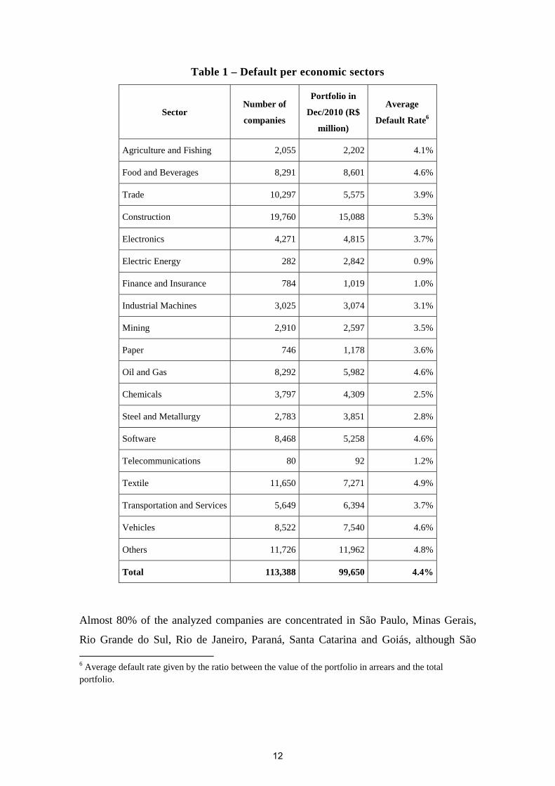
Table 1 – Default per economic sectors

Sector Number of

companies

Portfolio in

Dec/2010 (R$

million)

Average

Default Rate6

Agriculture and Fishing 2,055 2,202 4.1%

Food and Beverages 8,291 8,601 4.6%

Trade 10,297 5,575 3.9%

Construction 19,760 15,088 5.3%

Electronics 4,271 4,815 3.7%

Electric Energy 282 2,842 0.9%

Finance and Insurance 784 1,019 1.0%

Industrial Machines 3,025 3,074 3.1%

Mining 2,910 2,597 3.5%

Paper 746 1,178 3.6%

Oil and Gas 8,292 5,982 4.6%

Chemicals 3,797 4,309 2.5%

Steel and Metallurgy 2,783 3,851 2.8%

Software 8,468 5,258 4.6%

Telecommunications 80 92 1.2%

Textile 11,650 7,271 4.9%

Transportation and Services 5,649 6,394 3.7%

Vehicles 8,522 7,540 4.6%

Others 11,726 11,962 4.8%

Total 113,388 99,650 4.4%

Almost 80% of the analyzed companies are concentrated in São Paulo, Minas Gerais,

Rio Grande do Sul, Rio de Janeiro, Paraná, Santa Catarina and Goiás, although São 6 Average default rate given by the ratio between the value of the portfolio in arrears and the total portfolio.

12

Paulo holds 48.5% of the total loan transactions. Regarding the level of default, the

Midwest has the highest credit overdue rate for over 90 days, with 5.63%, followed by

the North, Southeast, Northeast and South, with 4.61%, 4.14%, 3.87% and 3.68%

respectively.

Regarding the degree of loan concentration in financial institutions, about 85% of the

analyzed companies have loan transactions in up to four financial institutions, which

corroborates the concentration profile of the National Financial System. According to

company size, default is higher among micro firms, with a rate of 5.5%, which

decreases to 0.2% for large companies. This result is consistent with some findings in

literature (Bunn and Redwood (2003) and Jiménez and Saurina (2004), among others).

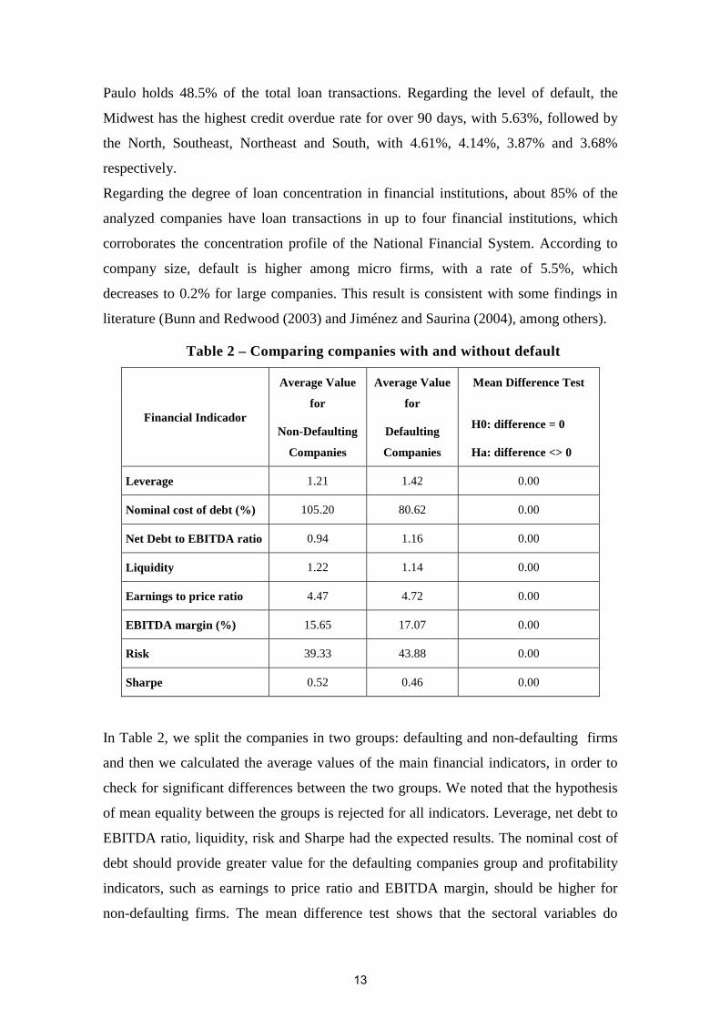
Table 2 – Comparing companies with and without default

Financial Indicador

Average Value

for

Non-Defaulting

Companies

Average Value

for

Defaulting

Companies

Mean Difference Test

H0: difference = 0

Ha: difference <> 0

Leverage 1.21 1.42 0.00

Nominal cost of debt (%) 105.20 80.62 0.00

Net Debt to EBITDA ratio 0.94 1.16 0.00

Liquidity 1.22 1.14 0.00

Earnings to price ratio 4.47 4.72 0.00

EBITDA margin (%) 15.65 17.07 0.00

Risk 39.33 43.88 0.00

Sharpe 0.52 0.46 0.00

In Table 2, we split the companies in two groups: defaulting and non-defaulting firms

and then we calculated the average values of the main financial indicators, in order to

check for significant differences between the two groups. We noted that the hypothesis

of mean equality between the groups is rejected for all indicators. Leverage, net debt to

EBITDA ratio, liquidity, risk and Sharpe had the expected results. The nominal cost of

debt should provide greater value for the defaulting companies group and profitability

indicators, such as earnings to price ratio and EBITDA margin, should be higher for

non-defaulting firms. The mean difference test shows that the sectoral variables do

13

differentiate default, and therefore can be interesting explanatory variables for default

probabilities in the absence of variables that relate directly to the company.

5. Methodology: the probit model of corporate default probability

The economic modeling underlying the empirical analysis is derived primarily from the

authors' previous article (Correa et al, 2011). Adapting the theoretical model there

described to the corporate case is not complicated. We can imagine that when a

company decides to take a loan, it intends to use the loan to implement an investment

project. The return on this project will depend on (i) the characteristics of the borrower

company, in particular, the risk rating assigned to it by the lender bank, as well as of the

loan transactions between this company and that lender, (ii) the macroeconomic

environment in which the company is inserted, in particular, the phase of the business

cycle, and, finally, (iii) other control variables associated with the economic sector of

the borrowing company.

The dependence of the project’s return on the phase of the cycle can be imagined by the

interdependence of existing projects in the economy. In recessionary phase, projects

developed by other companies may begin to present negative returns and consequently,

these companies can start to become delinquent. This delinquency, coming from

companies in the same industry or in different ones, may end up affecting the project’s

return of the original company and its ability to pay the loans.

We can then write, in a similar notation of the previous article, that:

, , , , ,

, , is the unobserved return of the borrowing company i, which took credit at the bank

j at time t. is a vector with observable personal characteristics of the borrower i and

its credit transactions. are macroeconomic variables at time t. ,′ are control

variables that can change among companies and across time. , and are parameters

vectors. is an unobserved individual effect of the company i. , , is a shock affecting

the project’s return, which is assumed to be independent and standard normally

distributed.

The borrowing company must obtain a minimum return α from its investment project in

order to be able to pay the loan that financed the project. Otherwise, the company will

become delinquent on that loan. However, the project’s payoff , , is not observed to

14

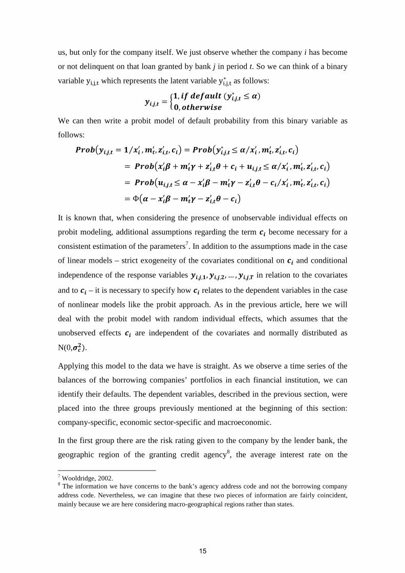
us, but only for the company itself. We just observe whether the company i has become

or not delinquent on that loan granted by bank j in period t. So we can think of a binary

variable y , , which represents the latent variable y , , as follows:

, , , , ,, We can then write a probit model of default probability from this binary variable as

follows:

, , ⁄ , , , , , , ⁄ , , , , , , , ⁄ , , , , , , , ⁄ , , , ,Ф ,

It is known that, when considering the presence of unobservable individual effects on

probit modeling, additional assumptions regarding the term become necessary for a

consistent estimation of the parameters7. In addition to the assumptions made in the case

of linear models – strict exogeneity of the covariates conditional on and conditional

independence of the response variables , , , , , , … , , , in relation to the covariates

and to – it is necessary to specify how relates to the dependent variables in the case

of nonlinear models like the probit approach. As in the previous article, here we will

deal with the probit model with random individual effects, which assumes that the

unobserved effects are independent of the covariates and normally distributed as

N(0, .

Applying this model to the data we have is straight. As we observe a time series of the

balances of the borrowing companies’ portfolios in each financial institution, we can

identify their defaults. The dependent variables, described in the previous section, were

placed into the three groups previously mentioned at the beginning of this section:

company-specific, economic sector-specific and macroeconomic.

In the first group there are the risk rating given to the company by the lender bank, the

geographic region of the granting credit agency8, the average interest rate on the

7 Wooldridge, 2002. 8 The information we have concerns to the bank’s agency address code and not the borrowing company address code. Nevertheless, we can imagine that these two pieces of information are fairly coincident, mainly because we are here considering macro-geographical regions rather than states.

15

company's operations in each lending institution, the percentage of collateralized

company's transactions at each institution, the number of financial institutions with

which the company has credit relationship, the balance of company's portfolio loans in

the national financial system and ultimately the economic sector where the company

operates. In the second group there are the variables representing the financial indicators

of the economic sectors where the companies operate, taken from Economática

database. Finally and representing the third group, we have variables associated to the

business cycle – the growth rate of GDP, the output gap, the growth rate of loans

granted to companies, the Ibovespa stock index change and the IPCA price index

change.9

6. Results

We estimated three specifications of this probit model to analyze the relationship

between corporate defaults and the business cycle. Tables 3 and 4 present the marginal

effects on the default probability for each model, evaluated on the average of the

explanatory variables. In Table 3, we present two initial specifications of the model,

considering only variables that are specific to the company (Model 1) and then adding

some controls that relate to the financial indicators of firms (Model 2). In Table 4, we

present the third specification based on four models (Models 3 to 7) that add variables

measuring the business cycle to Model 2. The difference among these five models

relates to the set of macroeconomic variables considered. For comparison, a linear

probability model with individual unobserved effect was also estimated by random

effect (Model 8).

9 All variables are described in more detail in Appendix.

16

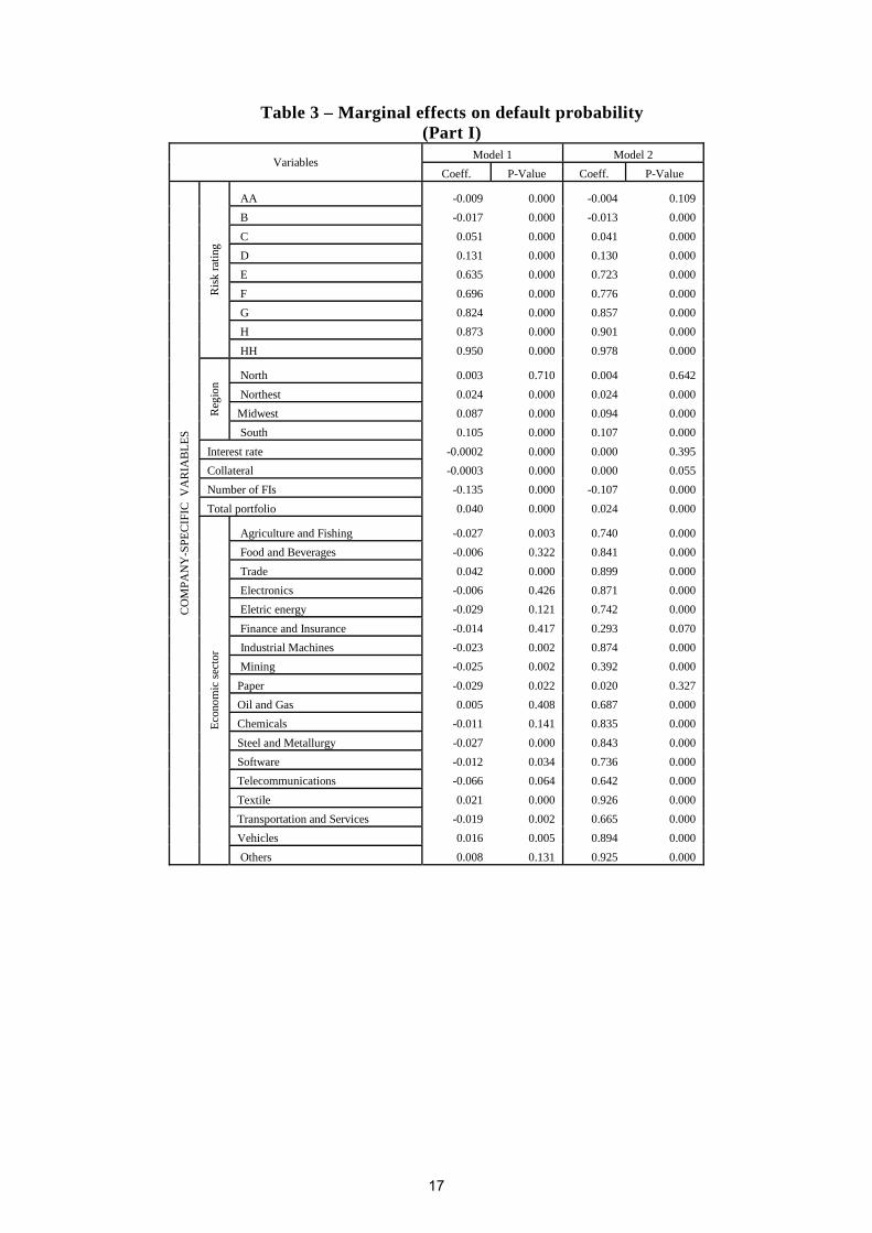
Table 3 – Marginal effects on default probability (Part I)

Variables Model 1 Model 2

Coeff. P-Value Coeff. P-Value C

OM

PAN

Y-S

PEC

IFIC

VA

RIA

BL

ES

Ris

k ra

ting

AA -0.009 0.000 -0.004 0.109

B -0.017 0.000 -0.013 0.000

C 0.051 0.000 0.041 0.000

D 0.131 0.000 0.130 0.000

E 0.635 0.000 0.723 0.000

F 0.696 0.000 0.776 0.000

G 0.824 0.000 0.857 0.000

H 0.873 0.000 0.901 0.000

HH 0.950 0.000 0.978 0.000

Reg

ion

North 0.003 0.710 0.004 0.642

Northest 0.024 0.000 0.024 0.000

Midwest 0.087 0.000 0.094 0.000

South 0.105 0.000 0.107 0.000

Interest rate -0.0002 0.000 0.000 0.395

Collateral -0.0003 0.000 0.000 0.055

Number of FIs -0.135 0.000 -0.107 0.000

Total portfolio 0.040 0.000 0.024 0.000

Eco

nom

ic s

ecto

r

Agriculture and Fishing -0.027 0.003 0.740 0.000

Food and Beverages -0.006 0.322 0.841 0.000

Trade 0.042 0.000 0.899 0.000

Electronics -0.006 0.426 0.871 0.000

Eletric energy -0.029 0.121 0.742 0.000

Finance and Insurance -0.014 0.417 0.293 0.070

Industrial Machines -0.023 0.002 0.874 0.000

Mining -0.025 0.002 0.392 0.000

Paper -0.029 0.022 0.020 0.327

Oil and Gas 0.005 0.408 0.687 0.000

Chemicals -0.011 0.141 0.835 0.000

Steel and Metallurgy -0.027 0.000 0.843 0.000

Software -0.012 0.034 0.736 0.000

Telecommunications -0.066 0.064 0.642 0.000

Textile 0.021 0.000 0.926 0.000

Transportation and Services -0.019 0.002 0.665 0.000

Vehicles 0.016 0.005 0.894 0.000

Others 0.008 0.131 0.925 0.000

17

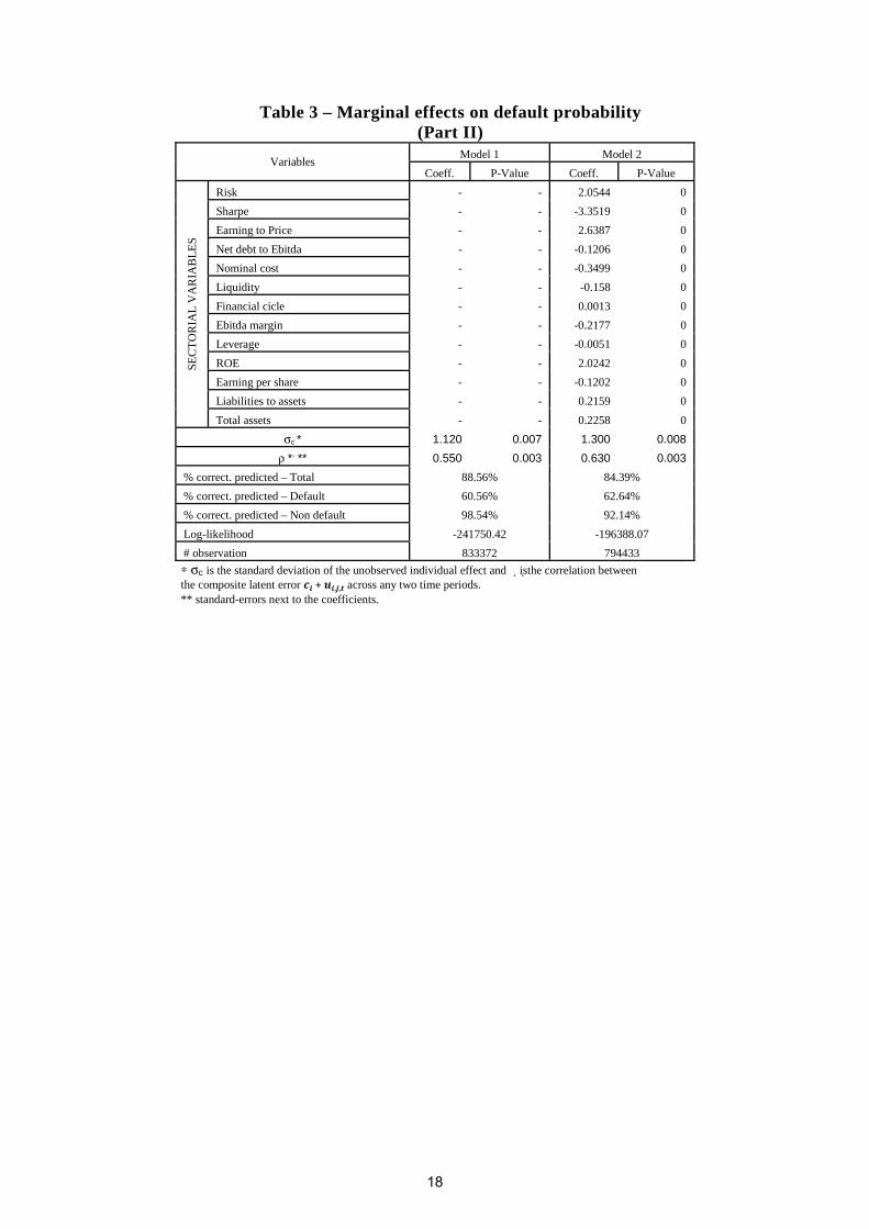
Table 3 – Marginal effects on default probability (Part II)

Variables Model 1 Model 2

Coeff. P-Value Coeff. P-Value

SEC

TO

RIA

L V

AR

IAB

LE

S Risk - - 2.0544 0

Sharpe - - -3.3519 0

Earning to Price - - 2.6387 0

Net debt to Ebitda - - -0.1206 0

Nominal cost - - -0.3499 0

Liquidity - - -0.158 0

Financial cicle - - 0.0013 0

Ebitda margin - - -0.2177 0

Leverage - - -0.0051 0

ROE - - 2.0242 0

Earning per share - - -0.1202 0

Liabilities to assets - - 0.2159 0

Total assets - - 0.2258 0

σc * 1.120 0.007 1.300 0.008

ρ *, ** 0.550 0.003 0.630 0.003

% correct. predicted – Total 88.56% 84.39%

% correct. predicted – Default 60.56% 62.64%

% correct. predicted – Non default 98.54% 92.14%

Log-likelihood -241750.42 -196388.07

# observation 833372 794433

∗ σc is the standard deviation of the unobserved individual effect and �isthe correlation between the composite latent error + , , across any two time periods. ** standard-errors next to the coefficients.

18

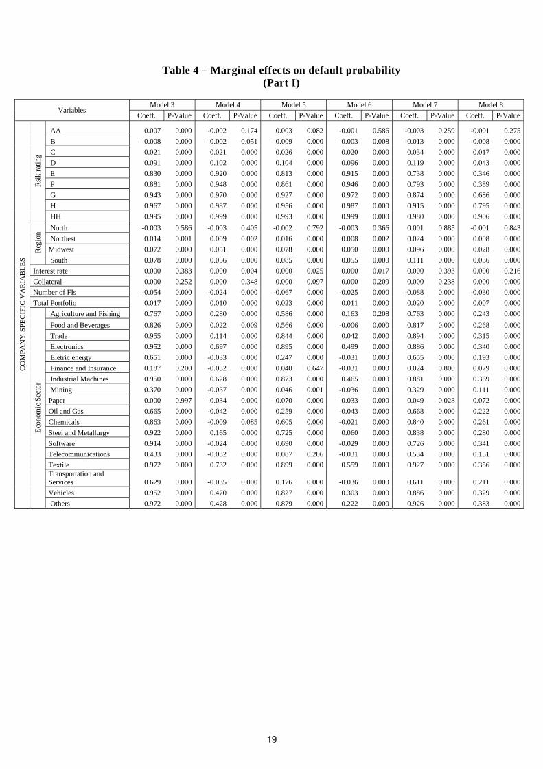
Table 4 – Marginal effects on default probability (Part I)

Variables Model 3 Model 4 Model 5 Model 6 Model 7 Model 8

Coeff. P-Value Coeff. P-Value Coeff. P-Value Coeff. P-Value Coeff. P-Value Coeff. P-Value

CO

MPA

NY

-SPE

CIF

IC V

AR

IAB

LE

S

Rsi

k ra

ting

AA 0.007 0.000 -0.002 0.174 0.003 0.082 -0.001 0.586 -0.003 0.259 -0.001 0.275

B -0.008 0.000 -0.002 0.051 -0.009 0.000 -0.003 0.008 -0.013 0.000 -0.008 0.000

C 0.021 0.000 0.021 0.000 0.026 0.000 0.020 0.000 0.034 0.000 0.017 0.000

D 0.091 0.000 0.102 0.000 0.104 0.000 0.096 0.000 0.119 0.000 0.043 0.000

E 0.830 0.000 0.920 0.000 0.813 0.000 0.915 0.000 0.738 0.000 0.346 0.000

F 0.881 0.000 0.948 0.000 0.861 0.000 0.946 0.000 0.793 0.000 0.389 0.000

G 0.943 0.000 0.970 0.000 0.927 0.000 0.972 0.000 0.874 0.000 0.686 0.000

H 0.967 0.000 0.987 0.000 0.956 0.000 0.987 0.000 0.915 0.000 0.795 0.000

HH 0.995 0.000 0.999 0.000 0.993 0.000 0.999 0.000 0.980 0.000 0.906 0.000

Reg

ion

North -0.003 0.586 -0.003 0.405 -0.002 0.792 -0.003 0.366 0.001 0.885 -0.001 0.843

Northest 0.014 0.001 0.009 0.002 0.016 0.000 0.008 0.002 0.024 0.000 0.008 0.000

Midwest 0.072 0.000 0.051 0.000 0.078 0.000 0.050 0.000 0.096 0.000 0.028 0.000

South 0.078 0.000 0.056 0.000 0.085 0.000 0.055 0.000 0.111 0.000 0.036 0.000

Interest rate 0.000 0.383 0.000 0.004 0.000 0.025 0.000 0.017 0.000 0.393 0.000 0.216

Collateral 0.000 0.252 0.000 0.348 0.000 0.097 0.000 0.209 0.000 0.238 0.000 0.000

Number of FIs -0.054 0.000 -0.024 0.000 -0.067 0.000 -0.025 0.000 -0.088 0.000 -0.030 0.000

Total Portfolio 0.017 0.000 0.010 0.000 0.023 0.000 0.011 0.000 0.020 0.000 0.007 0.000

Eco

nom

ic S

ecto

r

Agriculture and Fishing 0.767 0.000 0.280 0.000 0.586 0.000 0.163 0.208 0.763 0.000 0.243 0.000

Food and Beverages 0.826 0.000 0.022 0.009 0.566 0.000 -0.006 0.000 0.817 0.000 0.268 0.000

Trade 0.955 0.000 0.114 0.000 0.844 0.000 0.042 0.000 0.894 0.000 0.315 0.000

Electronics 0.952 0.000 0.697 0.000 0.895 0.000 0.499 0.000 0.886 0.000 0.340 0.000

Eletric energy 0.651 0.000 -0.033 0.000 0.247 0.000 -0.031 0.000 0.655 0.000 0.193 0.000

Finance and Insurance 0.187 0.200 -0.032 0.000 0.040 0.647 -0.031 0.000 0.024 0.800 0.079 0.000

Industrial Machines 0.950 0.000 0.628 0.000 0.873 0.000 0.465 0.000 0.881 0.000 0.369 0.000

Mining 0.370 0.000 -0.037 0.000 0.046 0.001 -0.036 0.000 0.329 0.000 0.111 0.000

Paper 0.000 0.997 -0.034 0.000 -0.070 0.000 -0.033 0.000 0.049 0.028 0.072 0.000

Oil and Gas 0.665 0.000 -0.042 0.000 0.259 0.000 -0.043 0.000 0.668 0.000 0.222 0.000

Chemicals 0.863 0.000 -0.009 0.085 0.605 0.000 -0.021 0.000 0.840 0.000 0.261 0.000

Steel and Metallurgy 0.922 0.000 0.165 0.000 0.725 0.000 0.060 0.000 0.838 0.000 0.280 0.000

Software 0.914 0.000 -0.024 0.000 0.690 0.000 -0.029 0.000 0.726 0.000 0.341 0.000

Telecommunications 0.433 0.000 -0.032 0.000 0.087 0.206 -0.031 0.000 0.534 0.000 0.151 0.000

Textile 0.972 0.000 0.732 0.000 0.899 0.000 0.559 0.000 0.927 0.000 0.356 0.000 Transportation and Services 0.629 0.000 -0.035 0.000 0.176 0.000 -0.036 0.000 0.611 0.000 0.211 0.000

Vehicles 0.952 0.000 0.470 0.000 0.827 0.000 0.303 0.000 0.886 0.000 0.329 0.000

Others 0.972 0.000 0.428 0.000 0.879 0.000 0.222 0.000 0.926 0.000 0.383 0.000

19

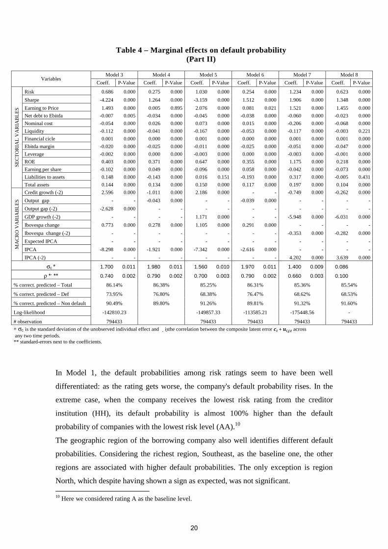
Table 4 – Marginal effects on default probability (Part II)

Variables Model 3 Model 4 Model 5 Model 6 Model 7 Model 8

Coeff. P-Value Coeff. P-Value Coeff. P-Value Coeff. P-Value Coeff. P-Value Coeff. P-Value

SEC

TO

RIA

L V

AR

IAB

LE

S

Risk 0.686 0.000 0.275 0.000 1.030 0.000 0.254 0.000 1.234 0.000 0.623 0.000

Sharpe -4.224 0.000 1.264 0.000 -3.159 0.000 1.512 0.000 1.906 0.000 1.348 0.000

Earning to Price 1.493 0.000 0.005 0.895 2.076 0.000 0.081 0.021 1.521 0.000 1.455 0.000

Net debt to Ebitda -0.007 0.005 -0.034 0.000 -0.045 0.000 -0.038 0.000 -0.060 0.000 -0.023 0.000

Nominal cost -0.054 0.000 0.026 0.000 0.073 0.000 0.015 0.000 -0.206 0.000 -0.068 0.000

Liquidity -0.112 0.000 -0.041 0.000 -0.167 0.000 -0.053 0.000 -0.117 0.000 -0.003 0.221

Financial cicle 0.001 0.000 0.000 0.000 0.001 0.000 0.000 0.000 0.001 0.000 0.001 0.000

Ebitda margin -0.020 0.000 -0.025 0.000 -0.011 0.000 -0.025 0.000 -0.051 0.000 -0.047 0.000

Leverage -0.002 0.000 0.000 0.000 -0.003 0.000 0.000 0.000 -0.003 0.000 -0.001 0.000

ROE 0.403 0.000 0.371 0.000 0.647 0.000 0.355 0.000 1.175 0.000 0.218 0.000

Earning per share -0.102 0.000 0.049 0.000 -0.096 0.000 0.058 0.000 -0.042 0.000 -0.073 0.000

Liabilities to assets 0.148 0.000 -0.143 0.000 0.016 0.151 -0.193 0.000 0.317 0.000 -0.005 0.431

Total assets 0.144 0.000 0.134 0.000 0.150 0.000 0.117 0.000 0.197 0.000 0.104 0.000

MA

CR

O V

AR

IAB

LE

S

Credit growth (-2) 2.596 0.000 -1.011 0.000 2.186 0.000 - - -0.749 0.000 -0.262 0.000

Output gap - - -0.043 0.000 - - -0.039 0.000 - - - -

Output gap (-2) -2.628 0.000 - - - - - - - - - -

GDP growth (-2) - - - - 1.171 0.000 - - -5.948 0.000 -6.031 0.000

Ibovespa change 0.773 0.000 0.278 0.000 1.105 0.000 0.291 0.000 - - - -

Ibovespa change (-2) - - - - - - - - -0.353 0.000 -0.282 0.000

Expected IPCA - - - - - - - - - - - -

IPCA -8.298 0.000 -1.921 0.000 -7.342 0.000 -2.616 0.000 - - - -

IPCA (-2) - - - - - - - - 4.202 0.000 3.639 0.000

σc * 1.700 0.011 1.980 0.011 1.560 0.010 1.970 0.011 1.400 0.009 0.086

ρ *, ** 0.740 0.002 0.790 0.002 0.700 0.003 0.790 0.002 0.660 0.003 0.100

% correct. predicted – Total 86.14% 86.38% 85.25% 86.31% 85.36% 85.54%

% correct. predicted – Def 73.95% 76.80% 68.38% 76.47% 68.62% 68.53%

% correct. predicted – Non default 90.49% 89.80% 91.26% 89.81% 91.32% 91.60%

Log-likelihood -142810.23 -149857.33 -113585.21 -175448.56 -

# observation 794433 794433 794433 794433 794433

∗ σc is the standard deviation of the unobserved individual effect and �isthe correlation between the composite latent error + , , across any two time periods. ** standard-errors next to the coefficients.

In Model 1, the default probabilities among risk ratings seem to have been well

differentiated: as the rating gets worse, the company's default probability rises. In the

extreme case, when the company receives the lowest risk rating from the creditor

institution (HH), its default probability is almost 100% higher than the default

probability of companies with the lowest risk level (AA).10

The geographic region of the borrowing company also well identifies different default

probabilities. Considering the richest region, Southeast, as the baseline one, the other

regions are associated with higher default probabilities. The only exception is region

North, which despite having shown a sign as expected, was not significant. 10 Here we considered rating A as the baseline level.

20

The average interest rate for the loan transactions was significant in explaining

delinquency. However, its marginal contribution to explain the default is virtually nil.

The percentage of company's collateralized transactions, although significant, also

appears with a very low negative coefficient, indicating that the more collateralized the

company loans are, the lower their default probability will be.11

The number of financial institutions with which the company has credit relationship

also proved significant in explaining delinquency. His sign, however, indicates that the

more creditors the company has, the lower their default probability. Repullo, Saurina

and Trucharte (2009) do not expect a negative sign in this case, imagining that the more

relationship a company has, the more restricted it might be in terms of liquidity and,

therefore, the greater its default probability. The negative relationship found only seems

reasonable if we think that a larger network of creditors available to a company might

mean that this company is well regarded by banks precisely because it has a history of

low defaults.

The total balance of the company’s loan portfolio also proved significant in explaining

delinquency. As this variable was created as a proxy for the size of the company, its

positive sign indicates that larger firms are more likely to default. Bonfim (2007) found

a similar result in her empirical database as well as in her regression models.

The results for the dummy variables identifying the economic sector of the borrowing

firm suggest that there are significant differences in the default probability for most

sectors. Of the 19 economic sectors considered, only eight were not significant to

differentiate the default probabilities of the respective sectors. Most of these non-

significant sectors presented much change in the sign of their respective coefficient

across the different models considered.

To measure the performance of the model, we calculated the percentage of correctly

predicted observations in three groups: total observations, observations in default and

observations not in default. We use a cutoff of 50% to define when the predicted

probability correctly predicts the company defaults. The correctly predicted percentages

from Model 1 are high (88%, 60% and 98% respectively) and, therefore, this model

seems to have already done a good job in terms of goodness of fit.

11 In fact, credit risk literature is controversial with respect to this signal. Some authors show that banks demand more collateral from those companies perceived as riskier. (Berger and Udell, 1990 and Jimenez, Salas and Saurina, 2006).

21

Even the company-specific variables having presented an important role to predict

default probability, their performance deserves to be revised considering controls that

relate to financial indicators of the companies. As our data do not allow us to identify

the company name, we had to deal with financial indicators representing the economic

sectors of each company. Therefore, in Model 2, we add to Model 1 indicators of

liquidity, profitability, efficiency, solvency and leverage.

Generally, the signals and the significance of the firm-specific variables remained

robust. This time, however, only two economic sectors were not significant to explain

the companies’ default, namely: Finance/Insurance and Paper. All others sectors had

default probabilities higher than the basal one (Construction). The financial variables

introduced were all significant, but not all of them had signal as expected. However, the

model performance in terms of percentage of observations correctly predicted remained

high: 84% for total observations, 62% for observations in default and 92% for

observations not in default. So this model also had a high goodness of fit. Therefore, we

decided to keep all financial variables in the following specification.

In the third specification, we add macroeconomic variables, to evaluate the effect of the

business cycle on corporate defaults (Models 3 to 7). These models differ with respect

to the lags of the variables considered. The variables are the GDP growth rate, the

output gap (used instead of GDP growth), the growth rate of loans granted to firms, the

Ibovespa stock index change and the IPCA price index change. In fact, we noted that

the effect of the cycle variables on default is not contemporary, since Model 7, which

considers all variables lagged two quarters, showed the best results in terms of expected

signals and significance of the macroeconomic variables.

In general, the signals and the significance of the existing variables remained robust

after the inclusion of macroeconomic variables. This time, however, only the financial

sector remained not significant to explain the companies’ defaults. All others presented

higher default probabilities than the Construction sector probabilities. The quality of the

model, in terms of percentage of correctly predicted observations, was not affected by

the inclusion of macroeconomic variables: 85% for total observations, 68% for

observations in default and 91% for observations in non default. Furthermore, in Model

7, all macroeconomic variables considered were significant, with expected signals and

strong marginal effects. Our estimates suggest that an additional percentage point in the

GDP growth rate reduces the default probability of a company in 6% two quarters

ahead. In the case of an inflation decrease, measured by the IPCA index, reduces the

22

default probability in 4% two quarters ahead. Regarding the granted credit, the effect on

reducing the corporate default probability is much lower: 0.74%. Finally, a positive

performance in the stock market, which generally reflects an improvement in the

companies’ financial condition, reduces their default probabilities in only 0.35% two

quarters ahead.

Model 8, which is the linear probability model used as a benchmark, provided the same

evidence of the best probit model (Model 7), namely: significant economic variables

and negative signals as expected. However, its marginal effects are somewhat smoother.

Tables 3 and 4 also show the standard deviation of the unobserved individual effect (σc)

and the correlation between the composite latent error + , , across any two time

periods (ρ). This correlation also measures the ratio of the variance of to the variance

of the composite error and that is why it is a useful measure of the relative importance

of the individual unobserved effect. Our estimates suggest that the individual effect

accounts for approximately 70% of the variance of the composite error and that this

effect is significantly different from zero in all models.

Finally, it is worth mentioning that other models were tested, considering, for example,

other business cycle variables such as the Selic interest rate, the expected inflation

rather than the actual inflation rate and the IBC-Br economic activity index, as well as

other time lags to evaluate the robustness of the results. We do not present these results

here because these models underperformed the presented ones, and several of its

variables were not significant and/or with expected signs.

An interesting extension to the present work is to consider some interactions in the

above specifications. Since the companies’ financial variables are also subject to

fluctuations over the business cycle, we can represent these co-movements adding

interactions between these variables and GDP growth to the model. Besides, we could

try to estimate separate models for different group of firms, according to their size, age

and economic sector for example. This would allow us to see if default probabilities are

driven by different factors in each of these groups.

23

7. Conclusion

This article focused on the relationship between credit default and macroeconomic

conditions in the corporate world, proposing to examine the validity of the first part of

the Basel II procyclicality argument for the Brazilian credit market. The idea of this

argument is that economic downturns would increase the credit default probability and

therefore would require a recomposition of capital requirements. In a second moment,

this consequent rearrangement of capital would lead to a credit crunch that would

further intensify the preexisting recession. The inability to separate credit supply from

credit demand with the available information prevents us from analyzing this second

part of the argument.

A probit model for the default probability was developed from a large and unique

database of micro credit taken from the Credit Information System of the Central Bank

of Brazil (SCR), from Economática’s financial indicators and from macroeconomic

variables. Our sample included information on more than 60,000 borrowing companies

and nearly 700 creditor financial institutions between 2005 and 2010.

In general, the variables built from micro credit transactions data were significant for

predicting default probabilities of companies. The risk ratings of the companies, the

geographic region of the granting credit agency and the economic sectors in which the

companies operate well differentiate their default probabilities. The model’s goodness

of fit, in terms of percentage of correctly predicted observations, remained high even

after the introduction of controls representative of sectoral financial indicators and of

macroeconomic variables.

When macro variables were introduced, the obtained results allowed us to conclude that

they have an important contribution to explain the delinquency of companies in the

Brazilian credit market. As expected, this contribution was stronger than in the already

studied case in a previous article by the authors on default from individuals12. The

macroeconomic variables with the greatest effect on corporate defaults were GDP

growth and inflation. Our estimates suggest that an additional percentage point in the

GDP growth rate reduces the companies’ default probability in 6% two quarters ahead.

Regarding an inflation decrease, measured by the IPCA price index change, it reduces

the default probability in 4% two quarters ahead.

12 Correa et al, 2011.

24

An interesting point for future research would be to explicitly include interactions

between macroeconomic variables and financial sector indicators in the above

modeling. We could also try to estimate separate models for different group of firms,

according to their size, age and economic sector for example. This would allow us to

see if default probabilities are driven by different factors in each of these groups.

Furthermore, a natural extension of the article would be to extend the sample period

used in order to include at least one complete economic cycle.

25

8. References

Bharath, S. T.; Shumway, T. Forecasting default with the Merton distance to default

model. Review of Financial Studies, 21, p. 1339-1369. 2008.

Bonfim, D. Credit risk drivers: evaluating the contribution of firm level information

and of macroeconomics dynamics. Journal of Banking and Finance, 33, p. 281-299.

2009.

Bunn, P. Redwood, V. Company accounts based modelling of business failures and the

implications for financial stability. Working Paper 210. Bank of England. 2003.

Correa, A. S., Marins, J. T. M., Neves, M. B. E., Silva, A.C.M. Credit Default and

Business Cycles: an empirical investigation of Brazilian retail loans. Working Paper

260. Central Bank of Brazil, 2011.

Duffie, D.; Saita, L.; Wang, K. Multi-period corporate default prediction. Journal of

Financial Economics, 83(3), p. 635-665. 2007.

Jacobson, T.; Lindé, J.; Roszbach, K. Firm default and aggregate fluctuations.

International Finance Discussion Papers, Board of Governors of the Federal Reserve

System, 1209. 2011.

Jarrow, R.A. Turnbull, S.M. The Intersection of Market and Credit Risk Journal of

Banking and Finance, 24: p. 271-299. 2000.

Jiménez, G., Saurina, J. Collateral, type of lender and relationship banking as

determinants of credit risk. Journal of Banking and Finance, 28, p.2191-2212. 2004.

Lando, D.; Nielsen, M. S. Correlation in Corporate Default: Contagion or Conditional

Dependence? Journal of Financial Intermediation, 19, p. 355-372. 2010.

Merton, R. C., On the Pricing of Corporate Debt: The Risk Structure of Interest Rates,

Journal of Finance, 29, n. 2, p. 449-470. 1974.

Pesaran, M.; Schuermann, H. T.; Treuler, B.J.; Weiner, S.M. Macroeconomic dynamics

and credit risk: a global perspective. Journal of Money, Credit and Banking, 38 (5), p.

1211-1261. 2006.

Repullo, R.; Saurina, J.; Trucharte, C. Mitigating the Procyclicality of Basel II.

Economic Policy, 25, p. 591-806. 2010.

26

Tang, D. Y.; Yan, H. Market conditions, default risk and credit spreads. Journal of

Banking and Finance, 24, p. 743-753. 2010.

Wooldridge, J. Econometric Analysis of Cross Section and Panel Data, 2002.

27

Appendix

Variables description

Leverage: quarterly sectoral variable that represents the median of debt capital and equity ratio. ROE: quarterly sectoral variable that represents the median of the return on equity. Earnings per share ratio: quarterly sectoral variable that represents the median of total earnings per company stock. Liabilities to total assets ratio: quarterly sectoral variable representing the median of liabilities and assets ratio. Total asset: quarterly sectoral variable that represents the median of total assets. Total portfolio: quarterly sectoral variable representing the sum of the client portfolio balances in all financial institutions with which he has credit transactions. Measured in logarithm terms. Financial cycle: quarterly sectoral variable that represents the median of the following expression: average collection period + average term of stock – average payment period. Net debt to Ebitda ratio: quarterly sectoral variable that represents the median of net debt and Ebitda ratio. Nominal cost of debt: quarterly sectoral variable that represents the median of interest paid and average debt ratio. Earning to price ratio: quarterly sectoral variable that represents the median of earnings and price ratio. Liquidity: quarterly sectoral variable that represents the median current assets and current liabilities ratio. Ebitda margin: quarterly sectoral variable that represents the median of Ebitda and net operating revenue ratio. Risk: quarterly sectoral variable that represents the median of the standard deviation of daily stock returns. Sharpe: quarterly sectoral variable that represents the median of the difference between the stock return and the risk-free return and stock returns standard deviation ratio. Default: quarterly variable of binary type being 1 if the client defaults in a given institution or 0 otherwise. The default criteria used was the existence of positive balance in overdue credits for more than 90 days and/or positive balance of written offs loans.

28

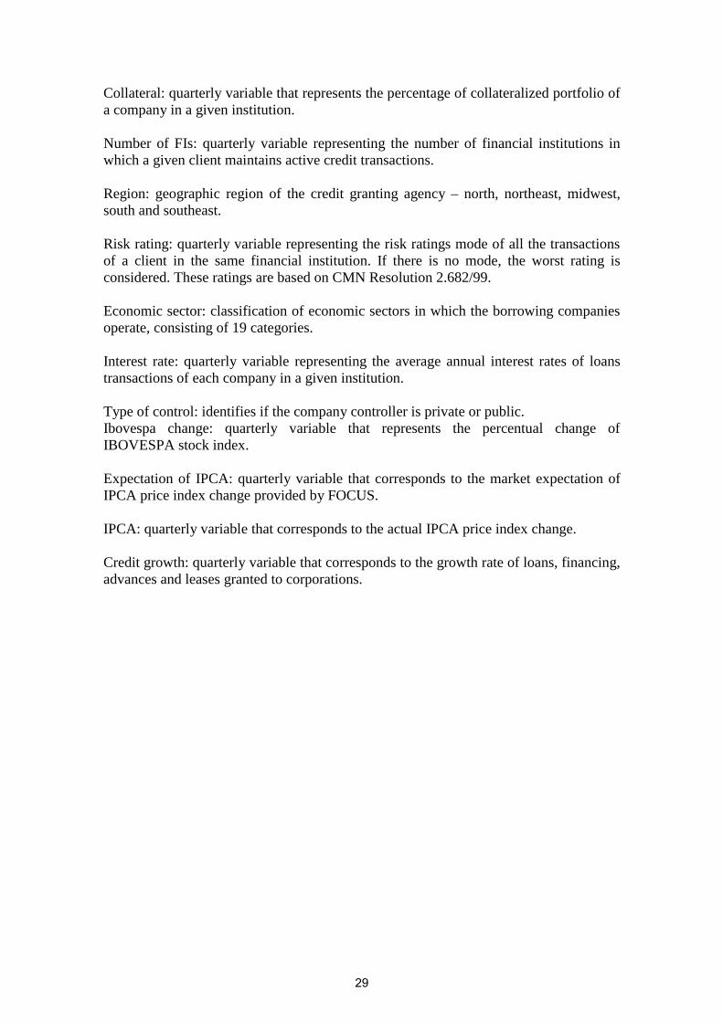
Collateral: quarterly variable that represents the percentage of collateralized portfolio of a company in a given institution. Number of FIs: quarterly variable representing the number of financial institutions in which a given client maintains active credit transactions. Region: geographic region of the credit granting agency – north, northeast, midwest, south and southeast. Risk rating: quarterly variable representing the risk ratings mode of all the transactions of a client in the same financial institution. If there is no mode, the worst rating is considered. These ratings are based on CMN Resolution 2.682/99. Economic sector: classification of economic sectors in which the borrowing companies operate, consisting of 19 categories. Interest rate: quarterly variable representing the average annual interest rates of loans transactions of each company in a given institution. Type of control: identifies if the company controller is private or public. Ibovespa change: quarterly variable that represents the percentual change of IBOVESPA stock index. Expectation of IPCA: quarterly variable that corresponds to the market expectation of IPCA price index change provided by FOCUS. IPCA: quarterly variable that corresponds to the actual IPCA price index change. Credit growth: quarterly variable that corresponds to the growth rate of loans, financing, advances and leases granted to corporations.

29

Banco Central do Brasil

Trabalhos para Discussão Os Trabalhos para Discussão do Banco Central do Brasil estão disponíveis para download no website

http://www.bcb.gov.br/?TRABDISCLISTA

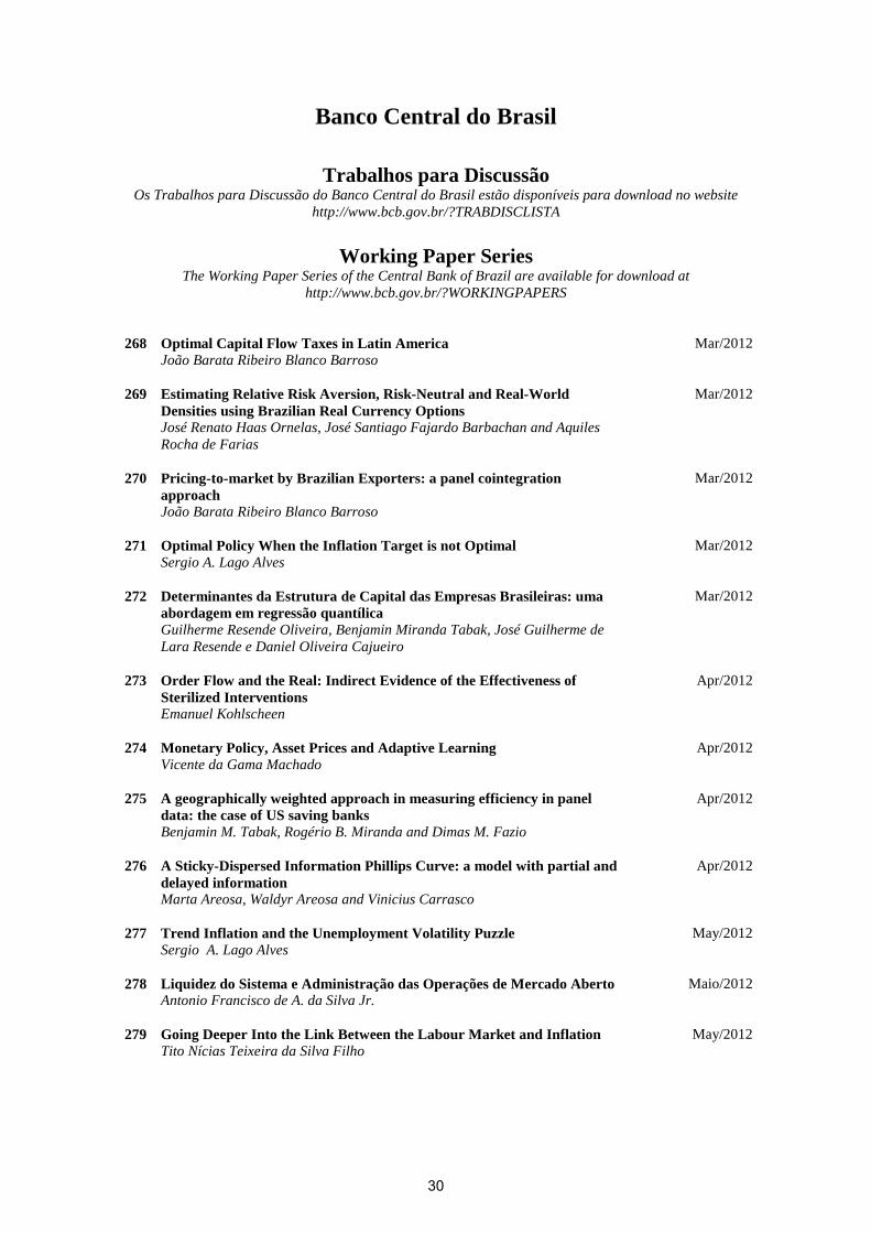
Working Paper Series

The Working Paper Series of the Central Bank of Brazil are available for download at http://www.bcb.gov.br/?WORKINGPAPERS

268 Optimal Capital Flow Taxes in Latin America

João Barata Ribeiro Blanco Barroso

Mar/2012

269 Estimating Relative Risk Aversion, Risk-Neutral and Real-World Densities using Brazilian Real Currency Options José Renato Haas Ornelas, José Santiago Fajardo Barbachan and Aquiles Rocha de Farias

Mar/2012

270 Pricing-to-market by Brazilian Exporters: a panel cointegration approach João Barata Ribeiro Blanco Barroso

Mar/2012

271 Optimal Policy When the Inflation Target is not Optimal Sergio A. Lago Alves

Mar/2012

272 Determinantes da Estrutura de Capital das Empresas Brasileiras: uma abordagem em regressão quantílica Guilherme Resende Oliveira, Benjamin Miranda Tabak, José Guilherme de Lara Resende e Daniel Oliveira Cajueiro

Mar/2012

273 Order Flow and the Real: Indirect Evidence of the Effectiveness of Sterilized Interventions Emanuel Kohlscheen

Apr/2012

274 Monetary Policy, Asset Prices and Adaptive Learning Vicente da Gama Machado

Apr/2012

275 A geographically weighted approach in measuring efficiency in panel data: the case of US saving banks Benjamin M. Tabak, Rogério B. Miranda and Dimas M. Fazio

Apr/2012

276 A Sticky-Dispersed Information Phillips Curve: a model with partial and

delayed information Marta Areosa, Waldyr Areosa and Vinicius Carrasco

Apr/2012

277 Trend Inflation and the Unemployment Volatility Puzzle

Sergio A. Lago Alves May/2012

278 Liquidez do Sistema e Administração das Operações de Mercado Aberto

Antonio Francisco de A. da Silva Jr. Maio/2012

279 Going Deeper Into the Link Between the Labour Market and Inflation

Tito Nícias Teixeira da Silva Filho May/2012

30

280 Educação Financeira para um Brasil Sustentável Evidências da necessidade de atuação do Banco Central do Brasil em educação financeira para o cumprimento de sua missão Fabio de Almeida Lopes Araújo e Marcos Aguerri Pimenta de Souza

Jun/2012

281 A Note on Particle Filters Applied to DSGE Models Angelo Marsiglia Fasolo

Jun/2012

282 The Signaling Effect of Exchange Rates: pass-through under dispersed information Waldyr Areosa and Marta Areosa

Jun/2012

283 The Impact of Market Power at Bank Level in Risk-taking: the Brazilian case Benjamin Miranda Tabak, Guilherme Maia Rodrigues Gomes and Maurício da Silva Medeiros Júnior

Jun/2012

284 On the Welfare Costs of Business-Cycle Fluctuations and Economic-Growth Variation in the 20th Century Osmani Teixeira de Carvalho Guillén, João Victor Issler and Afonso Arinos de Mello Franco-Neto

Jul/2012

285 Asset Prices and Monetary Policy – A Sticky-Dispersed Information Model Marta Areosa and Waldyr Areosa

Jul/2012

286 Information (in) Chains: information transmission through production chains Waldyr Areosa and Marta Areosa

Jul/2012

287 Some Financial Stability Indicators for Brazil Adriana Soares Sales, Waldyr D. Areosa and Marta B. M. Areosa

Jul/2012

288 Forecasting Bond Yields with Segmented Term Structure Models

Caio Almeida, Axel Simonsen and José Vicente Jul/2012

289 Financial Stability in Brazil

Luiz A. Pereira da Silva, Adriana Soares Sales and Wagner Piazza Gaglianone

Aug/2012

290 Sailing through the Global Financial Storm: Brazil's recent experience with monetary and macroprudential policies to lean against the financial cycle and deal with systemic risks Luiz Awazu Pereira da Silva and Ricardo Eyer Harris

Aug/2012

291 O Desempenho Recente da Política Monetária Brasileira sob a Ótica da Modelagem DSGE Bruno Freitas Boynard de Vasconcelos e José Angelo Divino

Set/2012

292 Coping with a Complex Global Environment: a Brazilian perspective on emerging market issues Adriana Soares Sales and João Barata Ribeiro Blanco Barroso

Oct/2012

293 Contagion in CDS, Banking and Equity Markets Rodrigo César de Castro Miranda, Benjamin Miranda Tabak and Mauricio Medeiros Junior

Oct/2012

31

294 Pesquisa de Estabilidade Financeira do Banco Central do Brasil Solange Maria Guerra, Benjamin Miranda Tabak e Rodrigo César de Castro Miranda

Out/2012

295 The External Finance Premium in Brazil: empirical analyses using state space models Fernando Nascimento de Oliveira

Oct/2012

296

Uma Avaliação dos Recolhimentos Compulsórios Leonardo S. Alencar, Tony Takeda, Bruno S. Martins e Paulo Evandro Dawid

Out/2012

297 Avaliando a Volatilidade Diária dos Ativos: a hora da negociação importa? José Valentim Machado Vicente, Gustavo Silva Araújo, Paula Baião Fisher de Castro e Felipe Noronha Tavares

Nov/2012

298 Atuação de Bancos Estrangeiros no Brasil: mercado de crédito e de derivativos de 2005 a 2011 Raquel de Freitas Oliveira, Rafael Felipe Schiozer e Sérgio Leão

Nov/2012

299 Local Market Structure and Bank Competition: evidence from the Brazilian auto loan market Bruno Martins

Nov/2012

Estrutura de Mercado Local e Competição Bancária: evidências no mercado de financiamento de veículos Bruno Martins

Nov/2012

300 Conectividade e Risco Sistêmico no Sistema de Pagamentos Brasileiro Benjamin Miranda Tabak, Rodrigo César de Castro Miranda e Sergio Rubens Stancato de Souza

Nov/2012

301 Determinantes da Captação Líquida dos Depósitos de Poupança Clodoaldo Aparecido Annibal

Dez/2012

302 Stress Testing Liquidity Risk: the case of the Brazilian Banking System Benjamin M. Tabak, Solange M. Guerra, Rodrigo C. Miranda and Sergio Rubens S. de Souza

Dec/2012

303 Using a DSGE Model to Assess the Macroeconomic Effects of Reserve Requirements in Brazil Waldyr Dutra Areosa and Christiano Arrigoni Coelho

Jan/2013

Utilizando um Modelo DSGE para Avaliar os Efeitos Macroeconômicos dos Recolhimentos Compulsórios no Brasil Waldyr Dutra Areosa e Christiano Arrigoni Coelho

Jan/2013

32