Critical bifurcation of shallow microtidal landformsin tidal flats and salt marshesSergio Fagherazzi*†, Luca Carniello‡, Luigi D’Alpaos‡, and Andrea Defina‡

*Department of Geological Sciences and School of Computational Science, Florida State University, Tallahassee, FL 32306; and ‡Dipartimento di IngegneriaIdraulica, Marittima, Ambientale e Geotecnica, Universita di Padova, Via Loredan 20, 35131 Padua, Italy

Edited by David Mohrig, Massachusetts Institute of Technology, Cambridge, MA, and accepted by the Editorial Board April 14, 2006 (received for reviewSeptember 25, 2005)

Shallow tidal basins are characterized by extensive tidal flats andsalt marshes that lie within specific ranges of elevation, whereasintermediate elevations are less frequent in intertidal landscapes.Here we show that this bimodal distribution of elevations stemsfrom the characteristics of wave-induced sediment resuspensionand, in particular, from the reduction of maximum wave heightcaused by dissipative processes in shallow waters. The conceptualmodel presented herein is applied to the Venice Lagoon, Italy, anddemonstrates that areas at intermediate elevations are inherentlyunstable and tend to become either tidal flats or salt marshes.

intertidal landforms

The distribution of elevations in shallow tidal basins such asthe Venice Lagoon in Italy (Fig 1, tidal range of 0.7 m) shows

that tidal f lats have differences in elevation of few tens ofcentimeters, with an average elevation between �0.50 and �1.00m above mean sea level (MSL), whereas salt marshes lie at anaverage elevation higher than �0.20 m, with some variabilitydictated by local sedimentological and ecological conditions(1–4). Few areas are located at intermediate elevations (i.e.,between �0.50 and �0.20 m), suggesting that the processesresponsible for sediment deposition and erosion produce eithertidal f lats or marshes but no landforms located at intermediateelevations. In the relatively pristine northern part of the VeniceLagoon, the most frequent bottom elevation is around �0.50 m(Fig. 2), similar to natural conditions in 1901 in the SouthernLagoon (Fig. 1 A). During the last century, anthropogenic causesproduced consistent bottom erosion in the Southern Lagoon,leading to a median elevation of approximately �1.00 m aboveMSL (Figs. 1B and 2). Nevertheless, all three distributions ofelevations show a relatively low frequency of elevations between0 and �0.5 m.

Typical conceptual and numerical models of salt-marsh for-mation envision a gradual transformation of sand flats andmudflats in response to sediment buildup and plant colonization(5–7). However, the evidence points to abrupt transitions to oneof two distinct stable outcomes. Salt marshes emerge from tidalf lats in locations where sedimentation is enhanced by lower tidalvelocities, higher sediment concentrations, or the shelteringeffects of splits and barrier islands (1, 8). Alternatively, in areaswith consistent sediment resuspension caused by a combinationof tidal f luxes and wind waves, tidal f lats are dominant. In tidalf lats, sediment deposition is balanced by erosion, and the bottomelevation is constantly maintained below MSL (9). Sedimentresuspension by wind waves is decisive, because tidal f luxes aloneare unable to produce the bottom shear stresses necessary tomobilize tidal-f lat sediments (10).

On the basis of a simplified model for wave generation inshallow water (10), we developed a conceptual model to studythe distribution of bottom shear stress as a function of elevation.The results are used to explain the bimodal distribution ofbathymetry in the Venice Lagoon.

Wind Waves in Shallow WaterWind waves are created by the transfer of energy from the windto the water surface. Starting from a flat water surface, wind

stresses generate waves that increase in height until the energydissipation caused by whitecapping, depth-induced breaking,and bottom friction limit the growth process (10, 11). Equilib-rium is reached when the energy generated by the wind actionequals the energy dissipated. In this situation, the height of thewave is the maximum possible for the particular bathymetry,meteorological forcing, and fetch length (the distance acrosswhich the wind can blow without land obstructions). Thus, waveheight is largely controlled by depth and increases in deep waters.

To compute wave height in shallow waters we study the localevolution of the wind-wave energy E, directly related to the waveheight by the linear theory. Wind-wave energy is described withan equation for the conservation of wave energy, which, formonochromatic waves, reads (10, 11)

�E��t � �cgE � S , [1]

where cg is wave-group celerity and S is a source term. In shallowbasins, waves quickly adapt to external forcing (i.e., �E��tbecomes negligible in a short period). In fact, strong dissipationlimits advection, so the wave field is essentially controlled bylocal energy balance. Moreover, the time required to reachequilibrium is short (10), so we can ignore the transient behavior.

The source term S includes wave growth by wind (Sw) andwave decay by bottom friction (Sbf), whitecapping (Swc), anddepth-induced breaking (Sb). Therefore, and as a first approx-imation, the conservation equation can be reduced to

Sw � Sbf � Swc � Sb. [2]

This equation states that equilibrium is reached when the energygenerated by the wind action equals the energy dissipation bybottom friction, whitecapping, and breaking. All terms in theequilibrium equation can be expressed as a function of waveenergy (10, 11), and the wave height can be calculated with aniterative algorithm. The terms in Eq. 2 are indicated in Table 1and were derived from widely adopted wave models (11). In ourmodel we implement Eq. 1 with a finite-elements algorithm. Toassess the influence of fetch length on wave generation, theadvection term in Eq. 1 was retained. The wave height was thencalculated along transects with constant bottom elevation, start-ing from a flat water surface and using Eq. 1 until steady statewas reached.

Bottom shear stresses are directly linked to wave height. In ourmodeling framework, the bottom shear stress (12) is given as

�b � 1�2 fw�wum2 with um � �H��T sinh�kY�� , [3]

Conflict of interest statement: No conflicts declared.

This paper was submitted directly (Track II) to the PNAS office. D.M. is a guest editor invitedby the Editorial Board.

Abbreviation: MSL, mean sea level.

†To whom correspondence should be addressed. E-mail: sergio@csit.fsu.edu.

© 2006 by The National Academy of Sciences of the USA

www.pnas.org�cgi�doi�10.1073�pnas.0508379103 PNAS � May 30, 2006 � vol. 103 � no. 22 � 8337–8341

GEO

LOG

Y

Dow

nloa

ded

by g

uest

on

Nov

embe

r 14

, 202

1

where fw is a friction factor and um is the maximum horizontalorbital velocity at the bottom associated with the wave. um

directly depends on wave height H and water depth Y so that, fora given water depth, higher waves produce larger bottom shearstresses. The rate of sediment erosion is supposed to be directlyproportional to the difference between bottom shear stress andthe critical shear stress for sediment erosion (7, 13):

R � A��b � �cr��, [4]

where R is the erosion rate, A is a constant of proportionality,and � ranges from 1 for cohesive sediments to 1.5 for loosesediments. �cr is the critical shear stress for erosion. In our modelwe set �cr � 0.7 Pa after extensive field studies in the VeniceLagoon (14).

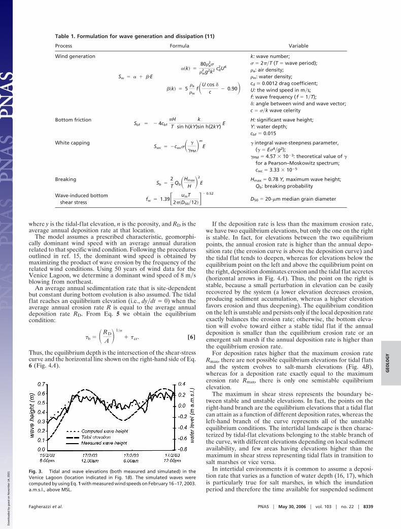
Bifurcation of Coastal LandformsWe obtain the shear-stress distribution from our model of wavegeneration by enforcing a monochromatic wave of period 2 s, thetypical value of wind waves in the Venice Lagoon. To test thevalidity of the model, we compare the wave height generated bya given wind speed with available wave measurements in theVenice Lagoon (Fig. 3). The model well reproduces the mea-sured values and shows a decreasing wave height in shallow waterdepths caused by the increased energy dissipation. In thissimulation, changes in water depth are produced by tidal oscil-lations in the lagoon.

Wave decay by bottom friction, whitecapping, and depth-induced breaking also affects bottom shear stresses, which arelinked to wave height through Eq. 3. However, shear stressesproduced by wind waves are not monotonically linked with waterdepth: they are limited in shallow water because of dissipativeprocesses, but they are also limited in deep water, where waveheight can be large but the bottom is too deep to be affected bywave oscillations (i.e., �b �cr).

Plotting the equilibrium bottom shear stress as a function ofwater depth for a given wind speed, we obtain a curve that peaksat an intermediate water depth (Fig. 4A). The curve is obtainedwithout considering the limiting effect of fetch length. Thismaximum of shear stress bears important consequences for themorphological transition from tidal f lats to salt marshes and forthe overall redistribution of sediments in shallow tidal basins.

On the basis of the relationship between shear stress andbottom elevation (Fig. 4A), we propose a model for the mor-phological evolution of salt marshes from tidal f lats.

The vertical evolution of tidal f lats is governed by the follow-ing differential equation:

�1 � n�dydt

� R � RD � A��b � �cr�� � RD, [5]

Fig. 1. Distribution of channels, salt marshes, and tidal flats in the Venice Lagoon in 1901 (A) and 2000 (B). The elevation is expressed in meters above MSL(a.m.s.l.). Areas within the circles are tidal-flat locations away from the channels in which the deposition rates are very low.

Fig. 2. Distribution of areas within the Venice Lagoon as a function ofelevation in 1901 and 2000. The elevation at which the vegetation startscolonizing the landscape was derived from ref. 16. AMSL, above MSL.

8338 � www.pnas.org�cgi�doi�10.1073�pnas.0508379103 Fagherazzi et al.

Dow

nloa

ded

by g

uest

on

Nov

embe

r 14

, 202

1

where y is the tidal-f lat elevation, n is the porosity, and RD is theaverage annual deposition rate at that location.

The model assumes a prescribed characteristic, geomorphi-cally dominant wind speed with an average annual durationrelated to that specific wind condition. Following the proceduresoutlined in ref. 15, the dominant wind speed is obtained bymaximizing the product of wave erosion by the frequency of therelated wind conditions. Using 50 years of wind data for theVenice Lagoon, we determine a dominant wind speed of 8 m�sblowing from northeast.

An average annual sedimentation rate that is site-dependentbut constant during bottom evolution is also assumed. The tidalf lat reaches an equilibrium elevation (i.e., dy�dt � 0) when theaverage annual erosion rate R is equal to the average annualdeposition rate RD. From Eq. 5 we obtain the equilibriumcondition:

�b � � RD

A � 1/�

� �cr. [6]

Thus, the equilibrium depth is the intersection of the shear-stresscurve and the horizontal line shown on the right-hand side of Eq.6 (Fig. 4A).

If the deposition rate is less than the maximum erosion rate,we have two equilibrium elevations, but only the one on the rightis stable. In fact, for elevations between the two equilibriumpoints, the annual erosion rate is higher than the annual depo-sition rate (the erosion curve is above the deposition curve) andthe tidal f lat tends to deepen, whereas for elevations below theequilibrium point on the left and above the equilibrium point onthe right, deposition dominates erosion and the tidal f lat accretes(horizontal arrows in Fig. 4A). Thus, the point on the right isstable, because a small perturbation in elevation can be easilyrecovered by the system (a lower elevation decreases erosion,producing sediment accumulation, whereas a higher elevationfavors erosion and thus deepening). The equilibrium conditionon the left is unstable and persists only if the local deposition rateexactly balances the erosion rate; otherwise, the bottom eleva-tion will evolve toward either a stable tidal f lat if the annualdeposition is smaller than the equilibrium erosion rate or anemergent salt marsh if the annual deposition rate is higher thanthe equilibrium erosion rate.

For deposition rates higher that the maximum erosion rateRmax, there are not possible equilibrium elevations for tidal f latsand the system evolves to salt-marsh elevations (Fig. 4B),whereas for a deposition rate exactly equal to the maximumerosion rate Rmax, there is only one semistable equilibriumelevation.

The maximum in shear stress represents the boundary be-tween stable and unstable elevations. In fact, the points on theright-hand branch are the equilibrium elevations that a tidal f latcan attain as a function of different deposition rates, whereas theleft-hand branch of the curve represents all of the unstableequilibrium conditions. The intertidal landscape is then charac-terized by tidal-f lat elevations belonging to the stable branch ofthe curve, with different elevations depending on local sedimentavailability, and few areas having elevations higher than themaximum in shear stress representing tidal f lats in transition tosalt marshes or vice versa.

In intertidal environments it is common to assume a deposi-tion rate that varies as a function of water depth (16, 17), whichis particularly true for salt marshes, in which the inundationperiod and therefore the time available for suspended sediment

Table 1. Formulation for wave generation and dissipation (11)

Process Formula Variable

Wind generation

Sw � � � �E

��k� �80�a

2

�w2 g2k2 cd

2U4

�k� � 5�a

�wf�U cos �

c� 0.90�

k: wave number; � 2��T (T � wave period);�a: air density;�w: water density;cd � 0.0012 drag coefficient;U: the wind speed in m�s;f: wave frequency ( f � 1�T);�: angle between wind and wave vector;c � �k wave celerity

Bottom frictionSbf � � 4cbf

�HT

ksin h(kY)sin h(2kY)

EH: significant wave height;Y: water depth;cbf � 0.015

White cappingSwc � �cwc� �

�PM�m

E� integral wave-steepness parameter,

(� � E4�g2);�PM � 4.57 10�3: theoretical value of �

for a Pearson–Moskowitz spectrum;cwc � 3.33 10�5

BreakingSb �

2T

Qb�Hmax

H �2

EHmax � 0.78 Y, maximum wave height;

Qb: breaking probability

Wave-induced bottomshear stress

fw � 1.39� umT2��D50�12��

� 0.52

D50 � 20- m median grain diameter

Fig. 3. Tidal and wave elevations (both measured and simulated) in theVenice Lagoon (location indicated in Fig. 1B). The simulated waves werecomputed by using Eq. 1 with measured wind speeds on February 16–17, 2003.a.m.s.l., above MSL.

Fagherazzi et al. PNAS � May 30, 2006 � vol. 103 � no. 22 � 8339

GEO

LOG

Y

Dow

nloa

ded

by g

uest

on

Nov

embe

r 14

, 202

1

to settle decreases with elevation when the marsh becomesemergent. Although this relationship is strictly true for bottomelevations within the tidal range, here we extend this assumptionto tidal f lats and determine the consequences of a decreasingsedimentation rate on equilibrium conditions. If we assume aconstant decrease in sedimentation rate and cohesive sediments(� � 1), the right-hand side of Eq. 6 can be graphically describedas a sloping line that intersects the shear-stress curve in twopoints (Fig. 4C). Again, we can separate the curve into twobranches (stable and unstable), but now the boundary betweenthe two branches is defined by the tangent point between thesloping line and the shear-stress curve. Because the line describ-ing Eq. 6 decreases with elevation, the separation point betweenthe two branches is located at a lower elevation than that in theconstant-deposition case. Similarly, it is possible to determinethe tidal-f lat equilibrium conditions for different sediment prop-erty (� � 1) and different monotonic relationships betweendeposition and elevation by substituting the sloping line with thecorresponding curve.

Discussion and ConclusionsThe presence of an unstable part in the curve of Fig. 4A is a veryreasonable explanation for the reduced frequency of areas atintermediate elevations (Fig. 2). However, the unstable regionpredicted by the model extends to �1.00 m above MSL, whereasfield evidence shows that the area frequency decreases onlybelow �0.50 m above MSL. The reasons for this discrepancy aremany fold: (i) Short wind fetch limits wave height. The distri-bution of bottom shear stress as a function of fetch lengthcalculated by using the finite-element model (10) solving Eq. 1indicates that the peak in shear stress shifts toward shallowerdepths (as shown in Fig. 4D). The shear stress peaks at �0.5 mfor a fetch of 1,000 m, the characteristic value for the VeniceLagoon, where frequent islands and marshes limit the distanceover which the wind blows. (ii) Tidal excursions periodically shiftthe water depth by approximately �0.35m. (iii) Deposition ratesmay be affected by water depth (Fig. 4C).

The decoupling of erosion and sedimentation in Eq. 5 ispartly justified by the fact that the average path of suspendedsediment during a tidal cycle is of the same order of magnitudeof the basin dimensions so that only a small fraction of erodedsediments is redeposited at the same location. In general, thedeposition rate at each point of the basin depends on sedimentredistribution driven by tidal currents, on the distance from themain tidal channels, and on allogenic sediment sources such asrivers and inlets. To determine the evolution of the entiresystem, our point analysis of tidal-f lat evolution must becoupled to a spatial description of sediment transport in thebasin so that the local sediment availability and averagedeposition rate are determined.

It is worth noting (see Fig. 2) that the encroachment ofhalophyte vegetation on salt marshes starts at �0.05 m in theVenice Lagoon and that the canopy is fully developed only above�0.15 m, as reported in detailed field measurements (18). Thus,halophyte vegetation does not affect the transition from tidalf lats to salt marshes for bottom elevations below MSL. Once thetidal f lat emerges, the vegetation rapidly colonizes the surface,increasing its elevation by sediment trapping and below-groundorganic production. Of particular importance for salt-marshequilibrium are the feedbacks between vegetation and accretion,including inorganic sediment trapping by vegetation (17, 19, 20).It is then the reduction in wave activity that is ultimatelyresponsible for the bifurcation of tidal landforms.

The bimodal distribution of tidal landforms is well defined forthe 1901 Southern Lagoon (see Fig. 2), whereas it is less evidentfor the 2000 bathymetry, with a less pronounced maximum forsalt marshes. This difference is due to the reduction in salt-marsharea occurred in the Venice Lagoon in recent decades but also

Fig. 4. Tidal flat equilibrium conditions. (A) Distribution of bottom shearstresses produced by wind waves as a function of elevation. The intersectionsbetween the shear-stress curve and the horizontal line (Eq. 6) are the equi-librium tidal-flat elevations. The curves are based on the assumption ofconstant annual deposition and a geomorphologically significant wind speedof 8 m�s, the typical value for tidal flats in the Venice Lagoon. The equilibriumpoint on the right is stable because small perturbations in elevation can berecovered by the system, whereas the equilibrium point on the left is unstable.(B) Tidal-flat equilibrium conditions as a function of different deposition rates.(C) Tidal-flat equilibrium conditions for sediment deposition decreasing withelevation. The stable branch of the curve extends to the tangent point withthe deposition line. (D) Shear-stress curves as a function of fetch length.

8340 � www.pnas.org�cgi�doi�10.1073�pnas.0508379103 Fagherazzi et al.

Dow

nloa

ded

by g

uest

on

Nov

embe

r 14

, 202

1

the presence of different plant species on the marsh platformthat expand the possible range of marsh elevations once thevegetation canopy is established (16).

Our model also predicts that wherever sediment supply isnegligibly small, any starting elevation on the curve shown in Fig.4 will evolve to a water depth of 2 to 2.5 m, the value at whichthe curve intersects the horizontal line of critical shear stress. Inthe Venice Lagoon, a negligible deposition occurs near thedivides separating the basins of Chioggia, Malamocco, and Lido,which are away from the large channels carrying the sediments.As expected, these two locations, where wind waves are notfetch-limited, are characterized by large tidal f lats that havemaintained a constant water depth of 2 to 2.5 m in the last twocenturies despite the radical morphological changes that oc-curred in the Venice Lagoon (Fig. 1, circled locations).

The proposed conceptual model indeed can explain andpredict evolutionary trends of the Venice Lagoon. In basinlocations with high deposition rates, the most frequent tidal-f latelevation is around �0.5 m, because for higher elevations the flatbecomes a salt marsh. If sediment availability is reduced (e.g., byremoving fluvial supply and promoting sediment loss), theequilibrium condition shifts toward lower elevations, as is hap-pening in the Southern Lagoon, where the dredging of the inletsand the construction of long jetties at the end of the 19th centuryreduced the median elevation of the flats to �1.00 m above MSL.

Conversely, if we increased the sediment availability (e.g., byrediverting rivers in the Venice Lagoon where they debouched

before the 15th century), the lagoon would start silting up butstill maintain an average tidal-f lat elevation around �0.5 mabove MSL. In fact, the lagoon infilling would occur through theformation of new salt marshes rather than by a generalizedbottom accretion.

The results of our analysis are valid in microtidal and me-sotidal environments away from tidal channels, where the re-suspension of bottom sediments is largely due to wind wavesrather than tidal currents. In locations with a high tidal excursionor in the channels dissecting the flats, tidal currents and theirspatial distribution are instead the chief geomorphic agents (10).Moreover, our analysis is limited to areas within tidal basins orbehind barrier islands and splits, which are sheltered from longwaves propagating from offshore, but can be also extended toflats lying in lakes and estuaries, where the tidal signal isnegligible.

We thank Mary Burke, Brad Murray, and an anonymous reviewer forcritical revision of the manuscript and the Ministero delle Infrastrutturee dei Trasporti (Magistrato alle Acque di Venezia) by way of itsconcessionary Consorzio Venezia Nuova for the field data essential tovalidate the model. This work was was supported by the Co.Ri.La.2004–2007 research program (linea 3.14, ‘‘Processi di erosione e sedi-mentazione nella laguna di Venezia,’’ and linea 3.18, ‘‘Tempi di resi-denza e dispersione idrodinamica nella laguna di Venezia’’), Office ofNaval Research Award N00014-05-1-0071, and National Science Foun-dation Award OCE-0505987.

1. Allen, J. R. L. (2000) Q. Sci. Rev. 19, 1155–1231.2. Friedrichs, C. T. & Perry, J. E. (2001) J. Coast. Res. 27, Special Issue, 7–37.3. Defina, A. (2000) Water Resour. Res. 36, 3251–3264.4. Fagherazzi, S., Bortoluzzi, A., Dietrich, W. E., Adami, A., Lanzoni, S., Marani,

M. & Rinaldo, A. (1999) Water Resour. Res. 35, 3891–3904.5. Beeftink, W. G. (1966) Wentia 15, 83–108.6. French, J. R. & Stoddart, D. R. (1992) Earth Surf. Processes Landforms 17,

235–252.7. Fagherazzi, S. & Furbish, D. J. (2001) J. Geophys. Res. Oceans 106, 991–1003.8. Dijkema, K. S. (1987) Z. Geomorph. 31, 489–499.9. Allen, J. R. L. & Duffy, M. J. (1998) Mar. Geol. 150, 1–27.

10. Carniello, L., Defina, A., Fagherazzi, S. & D’Alpaos, L. (2005) J. Geophys. Res.Earth Surf. 110, 10.1029�2004JF000232.

11. Booij, N., Ris, R. C. & Holthuijsen, L. H. (1999) J. Geophys. Res. Oceans 104,7649–7666.

12. Fredsoe, J. & Deigaard, R. (1992) Mechanics of Coastal Sediment Transport (Ad-vanced Series in Ocean Engineering, Vol. 3) (World Scientific, Singapore), p. 369.

13. Sanford, L. P. & Maa, J. P. Y. (2001) Mar. Geol. 1–2, 9–23.14. Amos, C. L., Bergamasco, A., Umgiesser, G., Cappucci, S., Cloutier, D., DeNat,

L., Flindt, M., Bonardi, M. & Cristante, S. (2004) J. Mar. Syst. 51, 211–241.15. Wolman, M. G. & Miller, J. P. (1960) J. Geol. 68, 54–74.16. French, J. R. (1993) Earth Surf. Processes Landforms 18, 63–81.17. Morris, J. T., Sundareshwar, P. V., Nietch, C. T., Kjerfve, B. & Cahoon, D. R.

(2002) Ecology 83, 2869–2877.18. Silvestri, S., Defina, A. & Marani, M. (2005) Estuar. Coast. Shelf Sci. 62,

119–130.19. Mudd, S. M., Fagherazzi, S., Morris, J. T. & Furbish, D. J. (2004) AGU Coast.

Estuar. Stud. 59, 165–189.20. D’Alpaos, A., Lanzoni, S., Mudd, S. M. & Fagherazzi, S. (2006) Estuar. Coast.

Shelf Sci., in press.

Fagherazzi et al. PNAS � May 30, 2006 � vol. 103 � no. 22 � 8341

GEO

LOG

Y

Dow

nloa

ded

by g

uest

on

Nov

embe

r 14

, 202

1