CryoSat-2 Precise Orbit Determination and Indirect ...deos.tudelft.nl/AS/ejo/ejo/text/cs2_cpr_main.pdf · to [email protected], DIODE Navigator and receiver

CryoSat-2 Precise OrbitDetermination and Indirect

Calibration of SIRAL

End of Commissioning Phase Report

E. Schrama, M. Naeije, Y. Yi, P. Visser, and C. Shum

Delft Institute for Earth-Oriented Space ResearchDelft University of TechnologyKluyverweg 1, 2629 HS DelftThe Netherlands C

This document was typeset with LATEX 2ε.The layout was designed by Remko Scharroo c© 1993–1999

Contents

1 Introduction 1

2 WP 310: Precise Orbit Determination (POD) 32.1 Introduction . . . . . . . . . . . . . . . . . . . . . . . . . . . . . . . . 3

2.1.1 POD infrastructure . . . . . . . . . . . . . . . . . . . . . . . . 32.1.2 Ground station coordinates for SLR and DORIS . . . . . . . 42.1.3 Satellite attitude model . . . . . . . . . . . . . . . . . . . . . 52.1.4 Solar radiation pressure model of Cryosat-2 . . . . . . . . . 62.1.5 Antenna phase center definitions . . . . . . . . . . . . . . . . 62.1.6 Satellite mass and center of gravity model . . . . . . . . . . 6

2.2 Precision orbit determination results for Cryosat-2 . . . . . . . . . . 62.2.1 SLR-only and DORIS-only solutions . . . . . . . . . . . . . . 8

2.3 External Orbit validation of Cryosat-2 . . . . . . . . . . . . . . . . . 82.4 Conclusions and recommendations . . . . . . . . . . . . . . . . . . . 9

2.4.1 Variations in Kdrag due to thermospheric density changes. . 102.5 Acknowledgments . . . . . . . . . . . . . . . . . . . . . . . . . . . . 102.6 Tables and figures . . . . . . . . . . . . . . . . . . . . . . . . . . . . . 10

3 WP 520: Indirect Calibration of SIRAL - Commissioning Phase 213.1 Work package tasks, inputs and outputs . . . . . . . . . . . . . . . . 213.2 Indirect calibration . . . . . . . . . . . . . . . . . . . . . . . . . . . . 223.3 Experiences with SIRAL LRM data . . . . . . . . . . . . . . . . . . . 233.4 L2LRM: surface anomaly compared . . . . . . . . . . . . . . . . . . 273.5 L2LRM conclusions . . . . . . . . . . . . . . . . . . . . . . . . . . . . 30

4 WP 530: Tide Gauge Calibration of SIRAL - Commissioning Phase 314.1 Work package tasks, inputs and outputs . . . . . . . . . . . . . . . . 314.2 Tide gauge calibration . . . . . . . . . . . . . . . . . . . . . . . . . . 324.3 Experiences with relative calibration of SIRAL using tide gauges . . 334.4 Tide gauge calibration conclusions . . . . . . . . . . . . . . . . . . . 35

Bibliography 37

Chapter 1

Introduction

In this report DEOS/A&S will report on the status of their activities at the endof the commissioning phase of the Cryosat-2 mission which was successfullylaunched on 8-april-2010. The work packages on which we report in this docu-ment are WP310 which concerns Precision Orbit Determination (POD) and workpackages WP520 and WP530 which are both related to the SIRAL altimeter inLRM as explained in Schrama et al. [2009].

Chapter 2

WP 310: Precise OrbitDetermination (POD)

This chapter describes status of precision orbit determination activities after com-pletion of the commissioning phase as described in contract Schrama et al. [2009].Within the framework of this contract we will compute trajectories of the Cryosat-2 satellite which are determined from DORIS and Satellite Laser Ranging (SLR)data for which the GEODYN-2 software is used, cf. Pavlis DE [2006]. In section 2.1we discuss the a summary of the assumed models, reference data and observationdatasets used for this study. In section 2.2 we report on the Cryosat-2 POD resultsobtained with the GEODYN-2 software. In section 2.3 we show the comparison toDORIS navigator orbit, Centre Nationales de Etudes Spatialles (CNES) MOE andPOE trajectories. In section 2.4 we present our conclusions and recommendationof this study.

2.1 Introduction

The section of astrodynamics and space missions within the faculty of aerospaceengineering at the Delft University of technology, short DEOS/A&S , worked onthe validation of Cryosat-2 orbits which are determined by DORIS and SLR.

Precision orbit determination at DEOS/A&S for Cryosat-2 is performed withthe help of the GEODYN-2 software developed by the space geodesy group at theGoddard Space Flight Center in Greenbelt Maryland. The provided tools are ex-tended with additional capabilities for processing new data types such as PRAREdata and altimeter crossover data. Furthermore DEOS/A&S developed new toolsto streamline DORIS satellite tracking data and also updating for instance earthorientation parameter (EOP) tables, magnetic field data, solar flux data and a va-riety of geophysical models.

The remainder of this section discusses the POD infrastructure in 2.1.1. Theimplementation of the ground station coordinates is described in section 2.1.2,the attitude model of Cryosat-2 is discussed in section 2.1.3, the solar radiationpressure (SRP) model of the satellite is in section 2.1.4 and the antenna offsetsare discussed in sub-section 2.1.5, a description of the satellite mass and center ofgravity is in section 2.1.6.

2.1.1 POD infrastructure

The precision orbit determination infrastructure for Cryosat-2 is as follows:

4 WP 310: Precise Orbit Determination (POD)

A front-end linux server with the functionality to retrieve 10s integratedDORIS Doppler and SLR information related to Cryosat-2 from public in-ternet sources. The main International Doris Service (IDS) repository forDORIS data is ftp://doris.ensg.ign.fr/pub/doris, a backup IDS repository isftp://cddis.gsfc.nasa.gov/pub/doris. The main source for retrieving satellitelaser ranging data is the Crustal Dynamics Data Information System (CD-DIS) accessible via ftp://cddis.gsfc.nasa.gov/pub/slr, and a backup SLR datasource at the Eurolas Data Center (EDC) accessible via ftp://ftp.dgfi.badw-muenchen.de/pub/slr.

A front-end linux server with the functionality to retrieve medium orbitephemeris (MOE) files, precision orbit ephemeris files (POE) files, satel-lite maneuver and mass data, quaternion data, DIODE navigator orbits,and receiver carrier phase data from ESA repositories dedicated to theCryosat-2 commissioning phase. MOE and POE orbit data arrives via ftpto [email protected], DIODE Navigator and receivercarrier phase data is retrieved by means of ftp to [email protected]. Spacecraft mass and maneuver events are received viasftp to [email protected], and star tracker data arrives viaFTP to [email protected]

A client linux workstation to receive the two line element (TLE) sets acquiredby North American Aerospace Defense Command (NORAD). This providesa backup mechanism for initializing the initial state vector for a new arc (i.e.a defined time window within which a trajectory will be reconstructed fromthe available tracking data). The latency of the TLE set is around 12 hours.Cryosat-2 TLE data is updated on a daily basis, it is considered to be a lowaccuracy data source that is only used as a backup facility in case there isno alternative source to provide an initial state vector. Relevant subsets ofthe TLE’s are maintained at website http://celestrak.com/NORAD/elements/,and an automated perl script at the client work station retrieves the TLE datatwice per day.

A client linux workstation to update the earth orientation parameters fromthe IERS repositories at www.iers.org and hpiers.obspm.fr. The client linuxworkstation is also used to update magnetic field and solar flux tables fromftp.ngdc.noaa.gov.

A client linux workstation on which DEOS/A&S installed the GEODYN-2software package which consists of GEODYN-2E, GEODYN-2S and the track-ing data formatter TDF. DEOS/A&S developed tools to convert native DORIS,SLR and CS2 quaternion data into input required for GEODYN-2.

2.1.2 Ground station coordinates for SLR and DORIS

POD depends on the availability of DORIS beacon and SLR tracking station co-ordinates. The International Terrestrial Reference Frame (ITRF) is a referencesystem which provides estimated coordinates and velocities of tracking stations.ITRF realizations are frequently updated and DEOS/A&S selected the most re-cent known coordinates for ground stations within the ITRF2008 reference sys-tem, see also ftp://itrf.ensg.ign.fr/pub/itrf/.

The majority of the DORIS ground station coordinates originate can be foundwithin ITRF2008. For the DORIS ground station coordinates that were not pro-vided in ITRF2008 DEOS/A&S selected the ITRF2005 coordinates. However, both

2.1 Introduction 5

for SLR and DORIS, ITRF2005 has some deficiencies and extensions (scaled ver-sions) are used during POD, see also Willis et al. [2009] and Ries [2010].

The biggest deficiency is that ITRF2005 coordinates are not available for quitea number of DORIS stations, because only stations through the end of 2005 areincluded while newer stations are not included in this reference frame solution.After 2006, the number of DORIS antenna’s has rapidly grown, hence it is impor-tant to update the coordinates. Moreover, due to more recent studies and meth-ods, more accurate station position and velocities can be obtained after 2005.

For POD applications, also additional information, such as periods of equip-ment malfunctioning and discontinuities, are required. These considerations leadto DPOD2005, which is an extension of ITRF2005. It includes all new DORIS sta-tions and is more reliable. The POD improvements rapidly and significantly in-crease after 2005. During the development phase for Cryosat-2 we encounteredsome issues with DPOD2005 version 1.4. These were communicated with the In-stitut de Physique du Globe de Paris and resulted in a new version: DPOD2005version 1.5 (4 December 2009). Since this is the latest standard for POD withDORIS stations, this model is implemented during Cryosat’s commissioningphase for DORIS stations one does not find in ITRF2008. To summarize the abovediscussion:

ITRF2008 coordinate definitions were assumed for DORIS beacons: ADFBARFB BADB BEMB CADB CHAB DIOB DJIB EASB EVEB FAIB FUTB GAVBGREB HBMB HEMB JIUB KETB KIUB KOLB LICB MAHB MALB MANBMATB METB MIAB MORB MSPB NOWB PDMB REUB REZB RIQB ROUBSAKB SALB SANB SCRB SPJB STJB SYPB THUB TLSB TRIB YASB YEMB.

DPOD2005 v1.5 coordinates were assumed for DORIS beacons: AMVB BETBCIDB CRQB GR3B KRBB KRVB RILB SODB ASEB PAUB.

ITRF2008 SLR tracking coordinate definitions were assumed for InternationalLaser Ranging Service (ILRS) sites: 1824 1873 1884 1893 7080 7090 7105 71107119 7124 7237 7249 7308 7403 7501 7810 7821 7824 7825 7832 7839 7840 78417845 7941 8834.

2.1.3 Satellite attitude model

The spacecraft body fixed coordinate frame (SBF) of Cryosat-2 is nominally ina 6 degree pitch down configuration as explained in Francis [2005]. Furthermorethere is a 4 degree yaw oscillation since 1 June, 2010. The used POD software doesnot provide the CS2 attitude law as a standard attitude model. For all satellitesthat don’t follow known (read: coded within the current version of the POD soft-ware) attitude laws there will be a need to specify the attitude of the spacecraftby means of a set of quaternions where the orientation of the SBF is presentedrelative to J2000.

Star tracker quaternion data was provided by ESA. Each of the three startrackers on board the Cryosat-2 satellite provides quaternions in its own cameraframe (SCF) relative to the inertial frame J2000. Internet access to the quaterniondata is explained in section 2.1.1, on 5-10-2010 16:25 we retrieved 4582 star trackerattitude files which follow the format:

CS_OPER_STR[1-3]ATT_*.TGZ

Each package contains HDR and DBL files and software was developed byDEOS/A&S to decode the star tracker quaternions and the corresponding time


tags with the help of information provided by Christopher Gotz at ESTEC Noord-wijk, see also document ESA [2008].

The resulting quaternions provide the orientation of the SCF relative to theinertial reference system J2000. In order to apply these quaternions to POD fur-ther processing is required. Therefore we transform the star tracker observedquaternions into quaternions that describe the orientation of the SBF to J2000 forwhich DEOS/A&S used transformation matrices provided by Francesco March-ese at ESOC in Darmstadt, see also document EADS [2009]. The end result aftertransformation and data compression of the dense star camera dataset is a dailyset of quaternions at 30 second intervals. Our daily sets of quaternions describethe orientation of the SBF relative to J2000. This set serves as input for the CS2attitude model during POD.

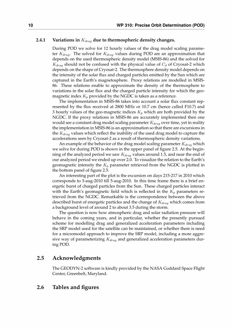
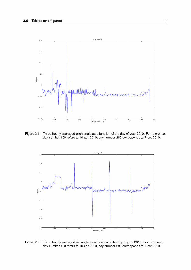
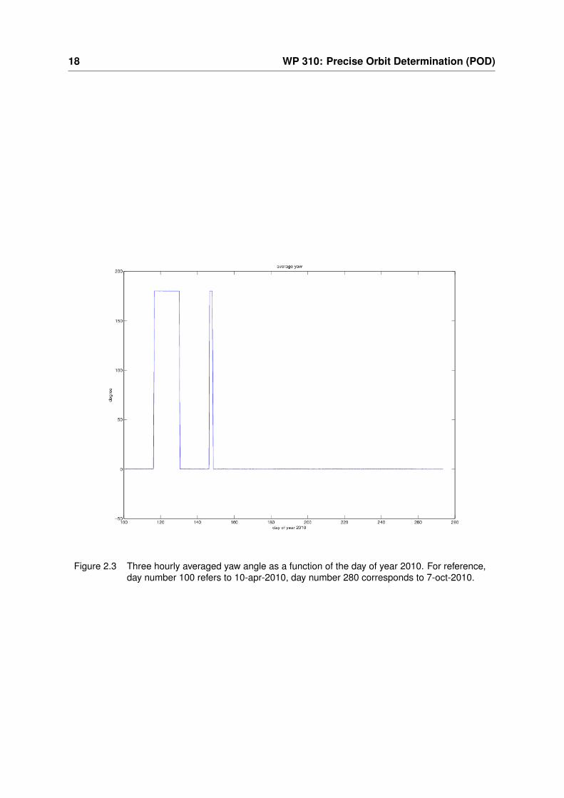
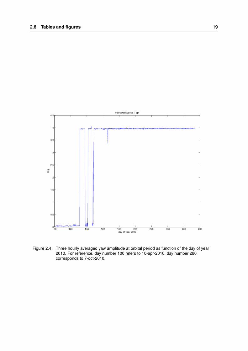
In order to validate our generated spacecraft quaternions we confronted theinterpolated set with a synthetic SBF retrieved from the Doris navigator orbitproduct as specified in section 2.1.1. This procedure allowed us to reconstruct thepitch, roll and yaw angles of Cryosat-2, and we confirmed that the satellite is ina 4 degree yaw steering mode since 28-5-2010 which is day number 148 in 2010,see figure 2.4. The period from launch up to 28-5-2010 is known for several orbitcorrections and isolated periods where the satellite was operating in a reverseyaw condition as can be seen in figures 2.1, 2.2 and 2.3.

2.1.4 Solar radiation pressure model of Cryosat-2

The solar radiation pressure (SRP) model of Cryosat-2 is a box only model relyingon input provided in document Francis [2005]. In total we defined 6 plates whichare a macro model approximation of the full spacecraft. The radiation pressurescaling coefficient Cr was determined to be 0.92 which followed from an estima-tion of this coefficient in the first week of June 2010.

2.1.5 Antenna phase center definitions

Document Francis [2005] is used to specify the phase centers of the 401.25 MHzand 2036.25 MHz Doris antennas and the SLR cube corner coordinates. The 2GHz phase center was chosen to represent carrier phase observations, and anionospheric free combination is formed from the observations at both frequen-cies. For the SLR cube corner on Cryosat-2 we used a constant offset of 19 mmwhich is an approximation of the elevation dependent correction as explained indocument Goetz [2006].

2.1.6 Satellite mass and center of gravity model

The position of the center of gravity within the satellite and its mass are frequentlyprovided by ESOC, see also section 2.1.1. The frequency of the updates dependson maintenance maneuvers and the cold gas usage for the Attitude and OrbitControl Sub-System (AOCS). We receive maneuver updates by e-mail, further-more they are provided by ESOC, see also section 2.1.1.

2.2 Precision orbit determination results for Cryosat-2

Given the fact that the CNES provides format 2.2 DORIS Doppler files since 1-June-2010 and that SLR data became available since 20-april-2010 we decided to

2.2 Precision orbit determination results for Cryosat-2 7

concentrate on the time frame 1-jun-2010 to 18-sep-2010. During POD we chosearcs to be not longer than 120 hours with an overlap of 24 hours. In addition weavoid to integrate equations of motion during a maneuver, see also section 2.1.6.

A second factor that determines the choice of the selected period is the avail-ability of IERS bulletin B data which contain polar motion and length of day pa-rameters. The update frequency of this product is 30 days which induces a latencyin our POD procedures.

A third factor is the availability of final values for geo-magnetic intensity andsolar flux constants which we retrieve from the National Geophysical Data Center(NGDC) via ftp.ngdc.noaa.gov. Both geophysical parameters are required withinthe atmospheric drag model and the solar radiation pressure model. Other accel-eration models used during POD are:

Potential coefficients of the Earth’s gravity model: EIGEN-5C up to degreeand order 70 including temporal gravity till degree and order 2.

Tidal modeling: h2 and l2 from latest International Earth Rotation Service(IERS) standards, EGM96 ocean tides, including the FES2004 ocean load tidemodel for the SLR core station set.

Thermospheric density model: MSIS-86

Lunar and planetary ephemeris: DE/LE-200, planetary gravity constants asin IAU2000.

Refraction modeling with the Marini Murray model. The ionospheric andtropospheric refraction for DORIS data is already provided by the CNES intheir format 2.2 ten second averaged range rate product.

General accelerations at one cycle per orbital revolution in the along-trackand cross track direction at daily intervals. This model absorbs unmodelledaccelerations on the spacecraft.

The atmospheric drag scaling parameter (Kdrag) is adjusted every twelvehours, the SRP model scaling parameter (Cr) is fixed at a constant value of0.92.

In addition we specify a number of technique specific parameters during POD:

The initial state vector for each arc was interpolated from the DORIS navigatororbit, and several adjustments are applied to reach convergence.

DORIS measurement biases and tropospheric scaling parameters are solvedby pass for each ground beacon.

We solve for an arc dependent clock offset of the DORIS satellite receiver.

Satellite ranging data is corrected for a 19 mm offset due to the phase centerdefinition of the cube corner on Cryosat-2. ILRS tracking station number 1893was corrected for a pass dependent range bias correction, 1873, 7090 and 7832are corrected for pass dependent time biases.

Dynamic editing techniques are used to remove spurious data-points in theSLR and the DORIS datasets. The relative weights in forming the normalequations involve an a priori choice of the observation standard deviation.To determine these weight we assumed an a priori standard deviation of 0.45mm/s for DORIS and 5 cm for laser ranging data.

Since the CNES did not apply beacon frequency offset corrections to theDORIS format 2.2 product we decided to use an a priori Doppler beacon fre-


quency offset table to assist the initialization of the dynamic editing proce-dures.

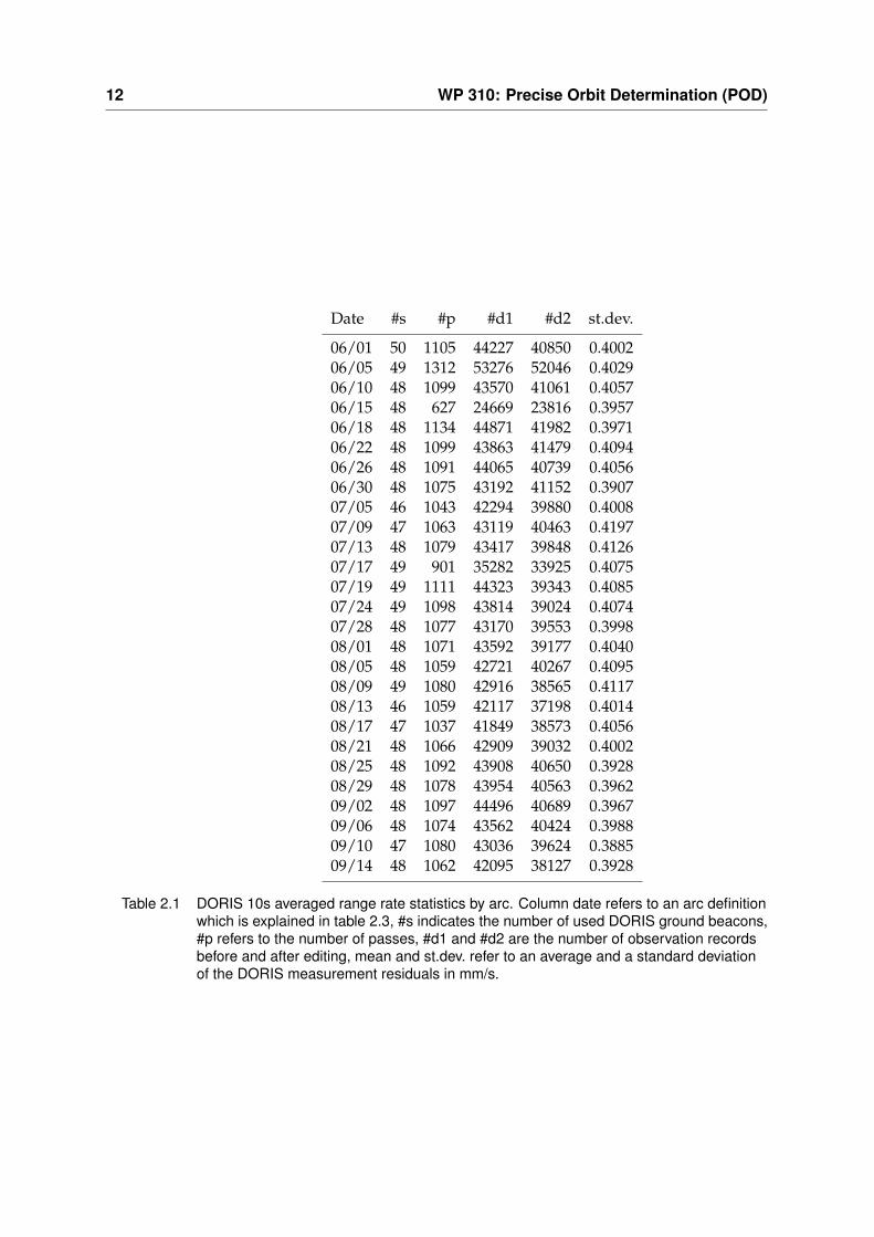
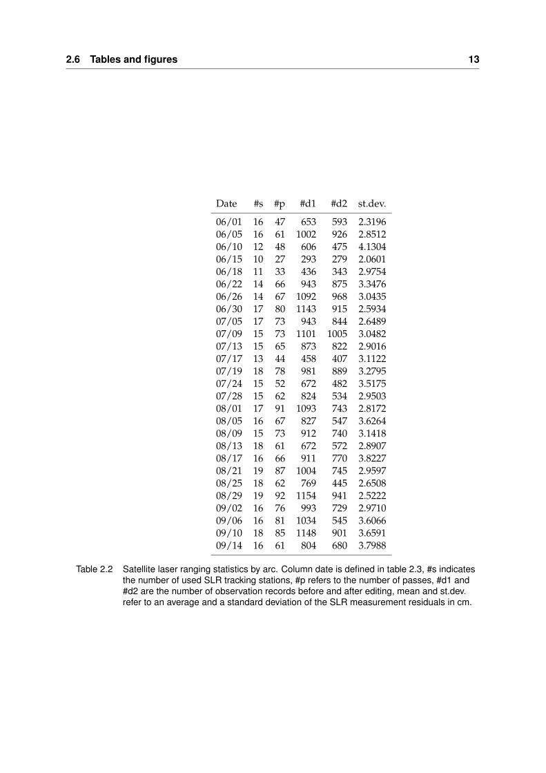
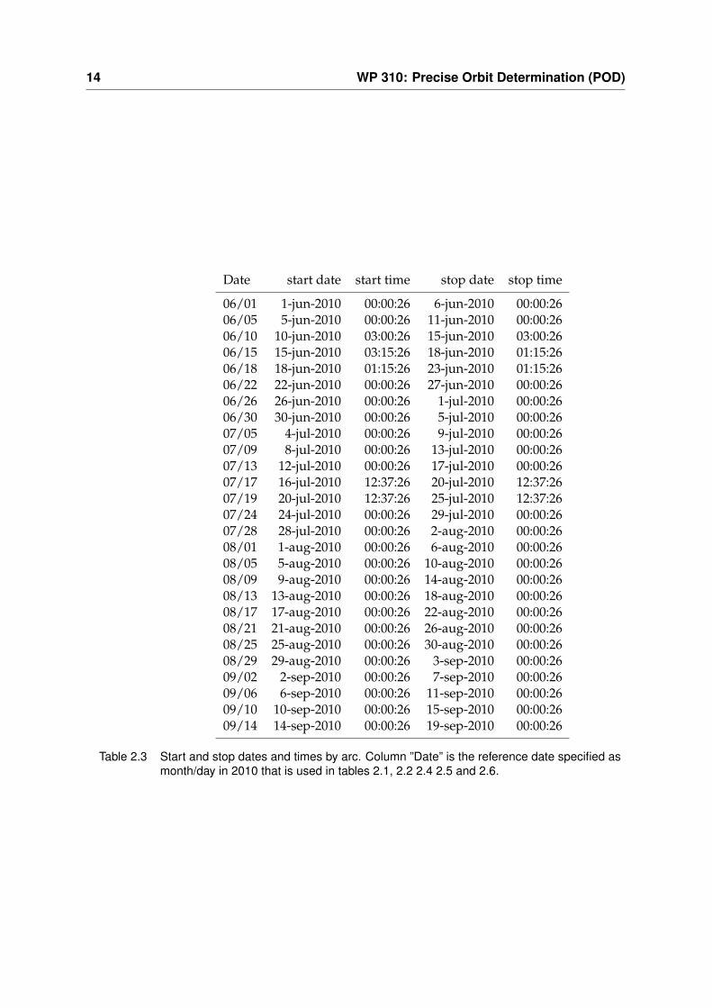
Table 2.1 shows the DORIS 10s average range rate residual statistics, and ta-ble 2.2 the SLR range rate residual statistics. Both tables apply to residuals for aselected arc. The conclusion is that the st.dev. of fit of the DORIS residuals be-comes ≈ 0.4 mm/s while the SLR st.dev. of fit is near ≈ 3.0 cm st.dev. In table 2.3we show the definitions of the arc begin and end times.

2.2.1 SLR-only and DORIS-only solutions

Our computed solutions significantly depend on information provided by theDORIS tracking system. To investigate this sensitivity we investigated a test arcstarting at 27-jun-2010 0hr UTC running to 30-jun-2010 0hr UTC. In this test pe-riod there is strong SLR coverage, and we can compute a SLR-only solution.

The difference of the SLR only solution compared to CNES POE solutionshows the following standard deviations: cross-track: 8.28 cm, radially: 3.29 cmand along track: 11.98 cm while the standard deviation of the three-dimensionaldifference is 14.93 cm. The DORIS-only solution show the following statistics:cross-track: 5.57 cm, radially: 1.31 and along track: 3.88 cm. The standard devi-ation of the three-dimensional difference to the CNES POE orbit is 6.92 cm. Forthe DORIS+SLR combination solution we get for the test arc: cross-track: 4.11 cm,radial: 1.31 cm and along track: 6.19 cm, in 3D the standard deviation is 7.55 cm.

The SLR-only solution is of course worse than what is typically obtained bya DORIS-only or a DORIS+SLR solution, but the SLR-only is a possible option toconsider if for some reason Cryosat-2 would ever lose DORIS tracking support.For the ERS-1 mission this was the situation due to the early demise of the PRAREtracking system. For ERS-1 DEOS/A&S was able to combine SLR tracking withthe altimeter cross-over data to improve the trajectory of ERS-1.

2.3 External Orbit validation of Cryosat-2

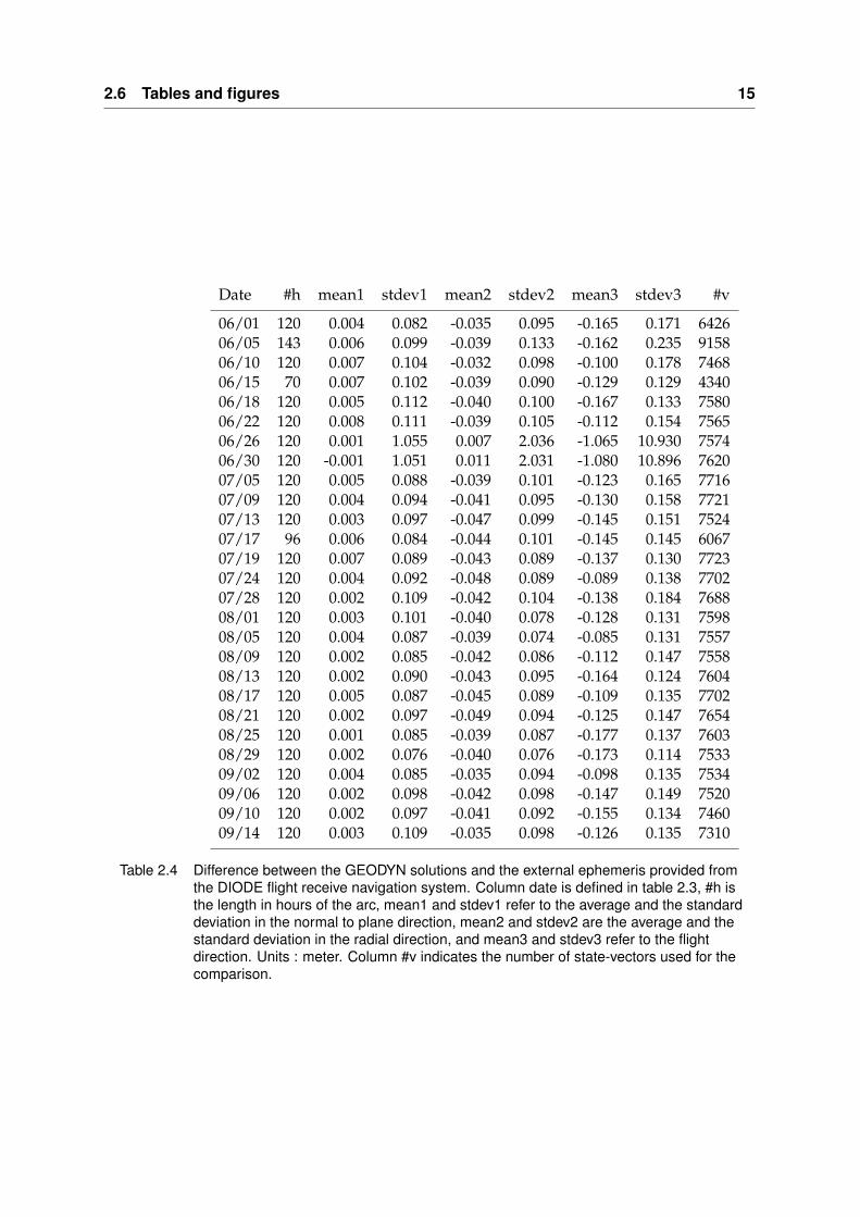
During the commissioning phase the CNES produced MOE and POE orbits forCryosat-2 while the on board flight receiver software (DIODE) produced real-time solutions. We retrieved these data from the CALVAL server as described insection 2.1.1 and computed differences as indicated in tables 2.4, 2.5 and 2.6.

On 30 June 2010 between 12:58:26 and 13:48:26 the DIODE system experiencedan anomaly which was reported by CNES to ESA. The DIODE system returnedonline on 13:48:26 UTC, the 3D error of the DIODE navigator solutions reducedto less than 10 m on 14:46:26 UTC. This anomalous situation explains the extremedifference between our solutions and the DIODE navigation solution on 30 June2010 which is in the overlap of arcs 06/26 and 06/30.

When we omit both anomalous arcs the differences between the Diode nav-igator orbits and our solutions is 9.36 cm st.dev. in the direction normal to theorbital plane which we will refer to as the cross-track direction. In the radial di-rection we find an agreement to within 9.43 cm st.dev, and in the in the traverseor along-track direction we get 14.87 cm st.dev, see also table 2.4. This means thata real-time solution of the DIODE system is better than the pre-flight specificationof the TOPEX/Poseidon altimeter which was launched by the National Aeronau-tics and Space Administration (NASA) in 1992. The DIODE navigator orbits area part of the AOCS on the Cryosat-2 mission, initialization of the star cameras

2.4 Conclusions and recommendations 9

depends on the DIODE navigator orbits, and also the satellite reference time iscontrolled by the ultra stable oscillator of the Doris system.

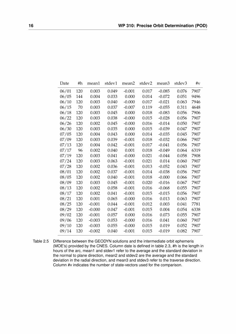
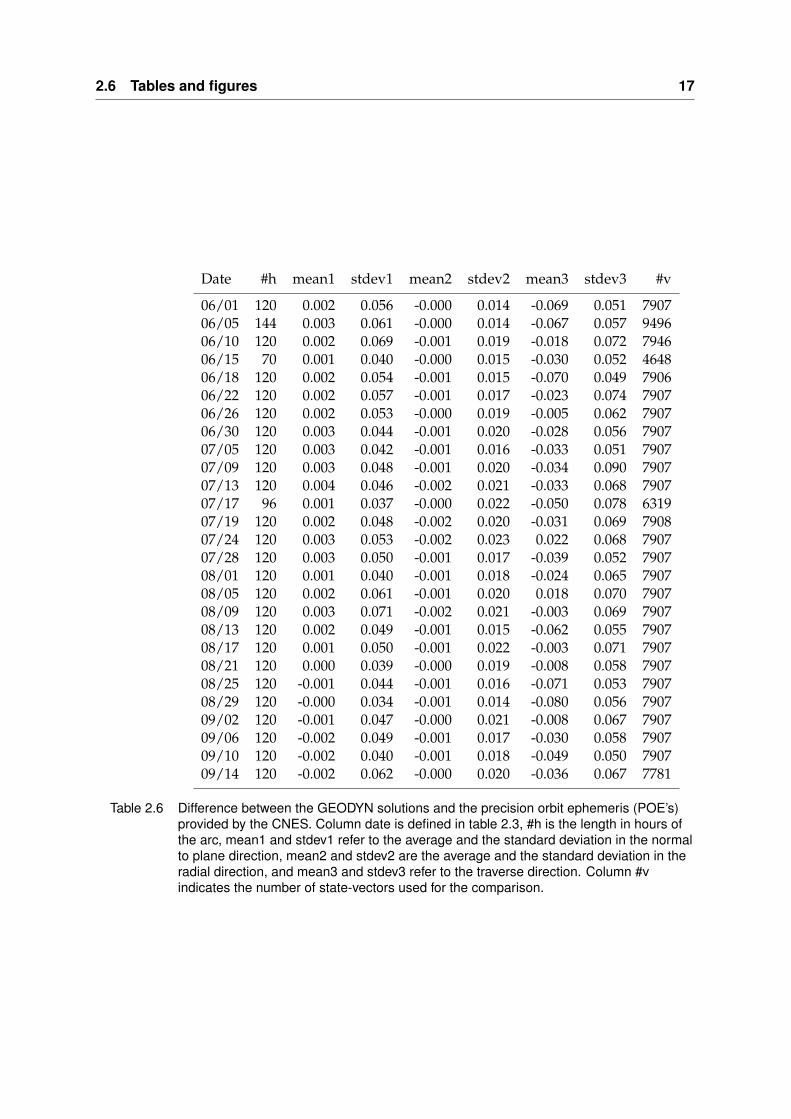
The CNES provided two additional products which are referred to as the MOEand the POE orbits. The MOE orbits agree to within 4.46 cm, 2.04 and 6.70 cmst.dev. in respectively the cross-track, the radial and the along-track direction. Intable 2.5 we show the individual mean and standard deviations for the arcs thatwe computed between 1-jun-2010 to 18-sep-2010. For the POE orbits we see anaverage standard deviation of 4.97 cm, 1.82 cm and 6.29 cm in the cross-track,the radial and the along track direction, the POE version of table 2.5 is shown intable 2.6. The MOE orbits are a clear improvement over the DIODE navigatorproduct and they are available within one day, the POE orbits have a latency of amonth, the POE orbits show a 10% improvement in the radial residuals comparedto the MOE’s.

2.4 Conclusions and recommendations

During the commissioning phase DEOS/A&S studied the complete POD pro-cessing chain which involves retrieval of satellite tracking data, spacecraft atti-tude data, and geophysical model data, including auxiliary data from varioussources. In the following we will briefly summarize the main findings during thecommissioning phase.

We demonstrated that the best agreement was found with the CNES POE or-bits. When we compare our arcs to these products we see an average standarddeviation of 4.97 cm, 1.82 cm and 6.29 cm in the cross-track, the radial and thealong track direction, the residuals by arc are shown in table 2.6. Our DORISmeasurement residuals are in the order of 0.4 mm/s for 10s averaged range rates,for the SLR residuals we have 3.0 cm st.dev.

We see already that the combination of SLR and DORIS orbits yields some-what deteriorated solutions compared to the DORIS only solution when we com-pare both our products with the CNES POE solution. This is work in progress,because it could point to issues that we may need to be improved in the opera-tional phase of Cryosat-2. Our recommendations for further research during theoperational phase are:

Improve on relative observation data weighting between SLR and DORIS.

Improve phase center offset maps of the DORIS antenna on Cryosat-2. Is therea dependency on the azimuth and elevation on the satellite looking at a DORISground beacons? Investigate also the phase center maps of the individualground beacons.

Investigate whether there are unresolved coordinate offsets on both theDORIS beacons and the SLR tracking stations.

Investigate the need to refine the SRP model used during POD, is there a needto improve the Cr constant?

Is a more aggressive parameterization of the drag and the 9 parameter generalacceleration model an option? For a discussion see section 2.4.1.

Can we confirm or improve accuracy of the Cryosat-2 orbits by means of min-imization of crossover residuals seen by the SIRAL LRM radar?


2.4.1 Variations in Kdrag due to thermospheric density changes.

During POD we solve for 12 hourly values of the drag model scaling parame-ter Kdrag. The solved for Kdrag values during POD are an approximation thatdepends on the used thermospheric density model (MSIS-86) and the solved forKdrag should not be confused with the physical value of Cd of Cryosat-2 whichdepends on the shape of Cryosat-2. The thermosphere density model depends onthe intensity of the solar flux and charged particles emitted by the Sun which arecaptured in the Earth’s magnetosphere. Proxy relations are modelled in MSIS-86. These relations enable to approximate the density of the thermosphere tovariations in the solar flux and the charged particle intensity for which the geo-magnetic index Kp provided by the NGDC is taken as a reference.

The implementation in MSIS-86 takes into account a solar flux constant rep-resented by the flux received at 2800 MHz or 10.7 cm (hence called F10.7) and3 hourly values of the geo-magnetic indices Kp which are both provided by theNGDC. If the proxy relations in MSIS-86 are accurately implemented then onewould see a constant drag model scaling parameter Kdrag over time, yet in realitythe implementation in MSIS-86 is an approximation so that there are excursions inthe Kdrag values which reflect the inability of the used drag model to capture theaccelerations seen by Cryosat-2 as a result of thermospheric density variations.

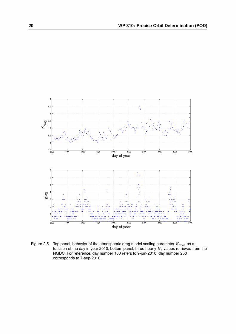
An example of the behavior of the drag model scaling parameter Kdrag whichwe solve for during POD is shown in the upper panel of figure 2.5. At the begin-ning of the analyzed period we saw Kdrag values around 1.5, and near the end ofour analyzed period we ended up over 2.0. To visualize the relation to the Earth’sgeomagnetic intensity the Kp parameter retrieved from the NGDC is plotted inthe bottom panel of figure 2.5.

An interesting part of the plot is the excursion on days 215-217 in 2010 whichcorresponds to 3-aug-2010 till 5-aug-2010. In this time frame there is a brief en-ergetic burst of charged particles from the Sun. These charged particles interactwith the Earth’s geomagnetic field which is reflected in the Kp parameters re-trieved from the NGDC. Remarkable is the correspondence between the abovedescribed burst of energetic particles and the change of Kdrag which comes froma background level of around 2 to about 3.5 during the storm.

The question is now how atmospheric drag and solar radiation pressure willbehave in the coming years, and in particular, whether the presently pursuedscheme for modelling drag and generalized acceleration parameters includingthe SRP model used for the satellite can be maintained, or whether there is needfor a micromodel approach to improve the SRP model, including a more aggre-sive way of parameterizing Kdrag and generalized acceleration parameters dur-ing POD.

2.5 Acknowledgments

The GEODYN-2 software is kindly provided by the NASA Goddard Space FlightCenter, Greenbelt, Maryland.

2.6 Tables and figures

2.6 Tables and figures 11

Figure 2.1 Three hourly averaged pitch angle as a function of the day of year 2010. For reference,day number 100 refers to 10-apr-2010, day number 280 corresponds to 7-oct-2010.

Figure 2.2 Three hourly averaged roll angle as a function of the day of year 2010. For reference,day number 100 refers to 10-apr-2010, day number 280 corresponds to 7-oct-2010.


Date #s #p #d1 #d2 st.dev.

06/01 50 1105 44227 40850 0.400206/05 49 1312 53276 52046 0.402906/10 48 1099 43570 41061 0.405706/15 48 627 24669 23816 0.395706/18 48 1134 44871 41982 0.397106/22 48 1099 43863 41479 0.409406/26 48 1091 44065 40739 0.405606/30 48 1075 43192 41152 0.390707/05 46 1043 42294 39880 0.400807/09 47 1063 43119 40463 0.419707/13 48 1079 43417 39848 0.412607/17 49 901 35282 33925 0.407507/19 49 1111 44323 39343 0.408507/24 49 1098 43814 39024 0.407407/28 48 1077 43170 39553 0.399808/01 48 1071 43592 39177 0.404008/05 48 1059 42721 40267 0.409508/09 49 1080 42916 38565 0.411708/13 46 1059 42117 37198 0.401408/17 47 1037 41849 38573 0.405608/21 48 1066 42909 39032 0.400208/25 48 1092 43908 40650 0.392808/29 48 1078 43954 40563 0.396209/02 48 1097 44496 40689 0.396709/06 48 1074 43562 40424 0.398809/10 47 1080 43036 39624 0.388509/14 48 1062 42095 38127 0.3928

Table 2.1 DORIS 10s averaged range rate statistics by arc. Column date refers to an arc definitionwhich is explained in table 2.3, #s indicates the number of used DORIS ground beacons,#p refers to the number of passes, #d1 and #d2 are the number of observation recordsbefore and after editing, mean and st.dev. refer to an average and a standard deviationof the DORIS measurement residuals in mm/s.


Date #s #p #d1 #d2 st.dev.

06/01 16 47 653 593 2.319606/05 16 61 1002 926 2.851206/10 12 48 606 475 4.130406/15 10 27 293 279 2.060106/18 11 33 436 343 2.975406/22 14 66 943 875 3.347606/26 14 67 1092 968 3.043506/30 17 80 1143 915 2.593407/05 17 73 943 844 2.648907/09 15 73 1101 1005 3.048207/13 15 65 873 822 2.901607/17 13 44 458 407 3.112207/19 18 78 981 889 3.279507/24 15 52 672 482 3.517507/28 15 62 824 534 2.950308/01 17 91 1093 743 2.817208/05 16 67 827 547 3.626408/09 15 73 912 740 3.141808/13 18 61 672 572 2.890708/17 16 66 911 770 3.822708/21 19 87 1004 745 2.959708/25 18 62 769 445 2.650808/29 19 92 1154 941 2.522209/02 16 76 993 729 2.971009/06 16 81 1034 545 3.606609/10 18 85 1148 901 3.659109/14 16 61 804 680 3.7988

Table 2.2 Satellite laser ranging statistics by arc. Column date is defined in table 2.3, #s indicatesthe number of used SLR tracking stations, #p refers to the number of passes, #d1 and#d2 are the number of observation records before and after editing, mean and st.dev.refer to an average and a standard deviation of the SLR measurement residuals in cm.


Date start date start time stop date stop time

06/01 1-jun-2010 00:00:26 6-jun-2010 00:00:2606/05 5-jun-2010 00:00:26 11-jun-2010 00:00:2606/10 10-jun-2010 03:00:26 15-jun-2010 03:00:2606/15 15-jun-2010 03:15:26 18-jun-2010 01:15:2606/18 18-jun-2010 01:15:26 23-jun-2010 01:15:2606/22 22-jun-2010 00:00:26 27-jun-2010 00:00:2606/26 26-jun-2010 00:00:26 1-jul-2010 00:00:2606/30 30-jun-2010 00:00:26 5-jul-2010 00:00:2607/05 4-jul-2010 00:00:26 9-jul-2010 00:00:2607/09 8-jul-2010 00:00:26 13-jul-2010 00:00:2607/13 12-jul-2010 00:00:26 17-jul-2010 00:00:2607/17 16-jul-2010 12:37:26 20-jul-2010 12:37:2607/19 20-jul-2010 12:37:26 25-jul-2010 12:37:2607/24 24-jul-2010 00:00:26 29-jul-2010 00:00:2607/28 28-jul-2010 00:00:26 2-aug-2010 00:00:2608/01 1-aug-2010 00:00:26 6-aug-2010 00:00:2608/05 5-aug-2010 00:00:26 10-aug-2010 00:00:2608/09 9-aug-2010 00:00:26 14-aug-2010 00:00:2608/13 13-aug-2010 00:00:26 18-aug-2010 00:00:2608/17 17-aug-2010 00:00:26 22-aug-2010 00:00:2608/21 21-aug-2010 00:00:26 26-aug-2010 00:00:2608/25 25-aug-2010 00:00:26 30-aug-2010 00:00:2608/29 29-aug-2010 00:00:26 3-sep-2010 00:00:2609/02 2-sep-2010 00:00:26 7-sep-2010 00:00:2609/06 6-sep-2010 00:00:26 11-sep-2010 00:00:2609/10 10-sep-2010 00:00:26 15-sep-2010 00:00:2609/14 14-sep-2010 00:00:26 19-sep-2010 00:00:26

Table 2.3 Start and stop dates and times by arc. Column ”Date” is the reference date specified asmonth/day in 2010 that is used in tables 2.1, 2.2 2.4 2.5 and 2.6.


Date #h mean1 stdev1 mean2 stdev2 mean3 stdev3 #v

06/01 120 0.004 0.082 -0.035 0.095 -0.165 0.171 642606/05 143 0.006 0.099 -0.039 0.133 -0.162 0.235 915806/10 120 0.007 0.104 -0.032 0.098 -0.100 0.178 746806/15 70 0.007 0.102 -0.039 0.090 -0.129 0.129 434006/18 120 0.005 0.112 -0.040 0.100 -0.167 0.133 758006/22 120 0.008 0.111 -0.039 0.105 -0.112 0.154 756506/26 120 0.001 1.055 0.007 2.036 -1.065 10.930 757406/30 120 -0.001 1.051 0.011 2.031 -1.080 10.896 762007/05 120 0.005 0.088 -0.039 0.101 -0.123 0.165 771607/09 120 0.004 0.094 -0.041 0.095 -0.130 0.158 772107/13 120 0.003 0.097 -0.047 0.099 -0.145 0.151 752407/17 96 0.006 0.084 -0.044 0.101 -0.145 0.145 606707/19 120 0.007 0.089 -0.043 0.089 -0.137 0.130 772307/24 120 0.004 0.092 -0.048 0.089 -0.089 0.138 770207/28 120 0.002 0.109 -0.042 0.104 -0.138 0.184 768808/01 120 0.003 0.101 -0.040 0.078 -0.128 0.131 759808/05 120 0.004 0.087 -0.039 0.074 -0.085 0.131 755708/09 120 0.002 0.085 -0.042 0.086 -0.112 0.147 755808/13 120 0.002 0.090 -0.043 0.095 -0.164 0.124 760408/17 120 0.005 0.087 -0.045 0.089 -0.109 0.135 770208/21 120 0.002 0.097 -0.049 0.094 -0.125 0.147 765408/25 120 0.001 0.085 -0.039 0.087 -0.177 0.137 760308/29 120 0.002 0.076 -0.040 0.076 -0.173 0.114 753309/02 120 0.004 0.085 -0.035 0.094 -0.098 0.135 753409/06 120 0.002 0.098 -0.042 0.098 -0.147 0.149 752009/10 120 0.002 0.097 -0.041 0.092 -0.155 0.134 746009/14 120 0.003 0.109 -0.035 0.098 -0.126 0.135 7310

Table 2.4 Difference between the GEODYN solutions and the external ephemeris provided fromthe DIODE flight receive navigation system. Column date is defined in table 2.3, #h isthe length in hours of the arc, mean1 and stdev1 refer to the average and the standarddeviation in the normal to plane direction, mean2 and stdev2 are the average and thestandard deviation in the radial direction, and mean3 and stdev3 refer to the flightdirection. Units : meter. Column #v indicates the number of state-vectors used for thecomparison.



06/01 120 0.003 0.049 -0.001 0.017 -0.085 0.076 790706/05 144 0.004 0.033 0.000 0.014 -0.072 0.051 949606/10 120 0.003 0.040 -0.000 0.017 -0.021 0.063 794606/15 70 0.003 0.037 -0.007 0.119 -0.055 0.311 464806/18 120 0.003 0.045 0.000 0.018 -0.083 0.056 790606/22 120 0.003 0.038 -0.000 0.015 -0.028 0.056 790706/26 120 0.002 0.045 -0.000 0.016 -0.014 0.050 790706/30 120 0.003 0.035 0.000 0.015 -0.039 0.047 790707/05 120 0.004 0.043 0.000 0.014 -0.035 0.045 790707/09 120 0.003 0.039 -0.001 0.018 -0.032 0.066 790707/13 120 0.004 0.042 -0.001 0.017 -0.041 0.056 790707/17 96 0.002 0.040 0.001 0.018 -0.049 0.064 631907/19 120 0.003 0.041 -0.000 0.021 -0.044 0.058 790807/24 120 0.003 0.063 -0.001 0.021 0.014 0.060 790707/28 120 0.002 0.036 -0.001 0.013 -0.052 0.043 790708/01 120 0.002 0.037 -0.001 0.014 -0.038 0.056 790708/05 120 0.002 0.040 -0.001 0.018 -0.000 0.066 790708/09 120 0.003 0.045 -0.001 0.020 -0.016 0.067 790708/13 120 0.002 0.058 -0.001 0.016 -0.068 0.055 790708/17 120 0.002 0.041 -0.001 0.015 -0.015 0.056 790708/21 120 0.001 0.065 -0.000 0.016 0.013 0.063 790708/25 120 -0.001 0.044 -0.001 0.012 0.003 0.041 778108/29 120 -0.000 0.047 -0.001 0.015 0.004 0.054 633809/02 120 -0.001 0.057 0.000 0.016 0.073 0.055 790709/06 120 -0.003 0.053 -0.000 0.016 0.041 0.060 790709/10 120 -0.003 0.055 -0.000 0.015 0.019 0.052 790709/14 120 -0.002 0.040 -0.001 0.015 -0.019 0.082 7907

Table 2.5 Difference between the GEODYN solutions and the intermediate orbit ephemeris(MOE’s) provided by the CNES. Column date is defined in table 2.3, #h is the length inhours of the arc, mean1 and stdev1 refer to the average and the standard deviation inthe normal to plane direction, mean2 and stdev2 are the average and the standarddeviation in the radial direction, and mean3 and stdev3 refer to the traverse direction.Column #v indicates the number of state-vectors used for the comparison.



06/01 120 0.002 0.056 -0.000 0.014 -0.069 0.051 790706/05 144 0.003 0.061 -0.000 0.014 -0.067 0.057 949606/10 120 0.002 0.069 -0.001 0.019 -0.018 0.072 794606/15 70 0.001 0.040 -0.000 0.015 -0.030 0.052 464806/18 120 0.002 0.054 -0.001 0.015 -0.070 0.049 790606/22 120 0.002 0.057 -0.001 0.017 -0.023 0.074 790706/26 120 0.002 0.053 -0.000 0.019 -0.005 0.062 790706/30 120 0.003 0.044 -0.001 0.020 -0.028 0.056 790707/05 120 0.003 0.042 -0.001 0.016 -0.033 0.051 790707/09 120 0.003 0.048 -0.001 0.020 -0.034 0.090 790707/13 120 0.004 0.046 -0.002 0.021 -0.033 0.068 790707/17 96 0.001 0.037 -0.000 0.022 -0.050 0.078 631907/19 120 0.002 0.048 -0.002 0.020 -0.031 0.069 790807/24 120 0.003 0.053 -0.002 0.023 0.022 0.068 790707/28 120 0.003 0.050 -0.001 0.017 -0.039 0.052 790708/01 120 0.001 0.040 -0.001 0.018 -0.024 0.065 790708/05 120 0.002 0.061 -0.001 0.020 0.018 0.070 790708/09 120 0.003 0.071 -0.002 0.021 -0.003 0.069 790708/13 120 0.002 0.049 -0.001 0.015 -0.062 0.055 790708/17 120 0.001 0.050 -0.001 0.022 -0.003 0.071 790708/21 120 0.000 0.039 -0.000 0.019 -0.008 0.058 790708/25 120 -0.001 0.044 -0.001 0.016 -0.071 0.053 790708/29 120 -0.000 0.034 -0.001 0.014 -0.080 0.056 790709/02 120 -0.001 0.047 -0.000 0.021 -0.008 0.067 790709/06 120 -0.002 0.049 -0.001 0.017 -0.030 0.058 790709/10 120 -0.002 0.040 -0.001 0.018 -0.049 0.050 790709/14 120 -0.002 0.062 -0.000 0.020 -0.036 0.067 7781

Table 2.6 Difference between the GEODYN solutions and the precision orbit ephemeris (POE’s)provided by the CNES. Column date is defined in table 2.3, #h is the length in hours ofthe arc, mean1 and stdev1 refer to the average and the standard deviation in the normalto plane direction, mean2 and stdev2 are the average and the standard deviation in theradial direction, and mean3 and stdev3 refer to the traverse direction. Column #vindicates the number of state-vectors used for the comparison.


Figure 2.3 Three hourly averaged yaw angle as a function of the day of year 2010. For reference,day number 100 refers to 10-apr-2010, day number 280 corresponds to 7-oct-2010.


Figure 2.4 Three hourly averaged yaw amplitude at orbital period as function of the day of year2010. For reference, day number 100 refers to 10-apr-2010, day number 280corresponds to 7-oct-2010.


Figure 2.5 Top panel, behavior of the atmospheric drag model scaling parameter Kdrag as afunction of the day in year 2010, bottom panel, three hourly Kp values retrieved from theNGDC. For reference, day number 160 refers to 9-jun-2010, day number 250corresponds to 7-sep-2010.

Chapter 3

WP 520: Indirect Calibration ofSIRAL - Commissioning Phase

This section deals with the work conducted for the calibration and validation ofthe CryoSat-2 Ocean product, or Low Resolution Mode (LRM) data and providesthe status at the end of the Commissioning Phase. (The LRM level 1b data formatis described in ACSL1b [2009] and the level 2 data in ACSL2 [2009].) This work,referred to as WP 520 in the ”CryoSat-2 Precise Orbit Determination and IndirectCalibration of SIRAL” project plan, entailed the analysis and identification of sys-tematic errors in the CryoSat-2 LRM observations, first estimation of range biasand the preliminary comparison with other operational altimeter satellites. Afull cross-calibration with Envisat, Jason-1 and Jason-2 though could not be per-formed due to not yet resolved (but understood and soon to be resolved) bugs inthe ground processing of the raw altimeter product. In spite of this, already veryuseful conclusions can be drawn from the analyses that at the same time helped toimprove the ground processing chain. We see this ”exercise” as work in progressand expect a continued research on data quality, range bias and time tag bias inthe Operational Phase. We acknowledge the need for a persistent monitoring ofthese biases in time to be able to provide insight in drift, which could be importantto be taken into account when using the data for the investigation of long-termchanges like sea level change, and or ice topography/volume change. In addi-tion, we expect that the altimeter (range) data can be used to assess the radial orbitaccuracy by generating crossover statistics which is a standard technique that weapply for ERS-1/2, Envisat, Topex/POSEIDON, Jason-1/2 and GFO. This is nowplanned for the Operational Phase. Meanwhile DEOS debugged its in-house soft-ware (RADS and applications) to address the latest issues with the CryoSat data.At this point, we are convinced that there is no need for adding altimeter dataas tracking information to the set of DORIS and SLR because these already pro-vide very consistent and accurate orbits. Altimetry is useful if there would be ashortage of tracking data, though the direct danger of adding altimetry would beleakage of ocean dynamics into the orbit.

3.1 Work package tasks, inputs and outputs

Tasks defined under WP 520:

LRM altimeter bias and time tag estimation in POD

LRM altimeter bias and time tag estimation by comparison with altimeter datafrom other satellites

22 WP 520: Indirect Calibration of SIRAL - Commissioning Phase

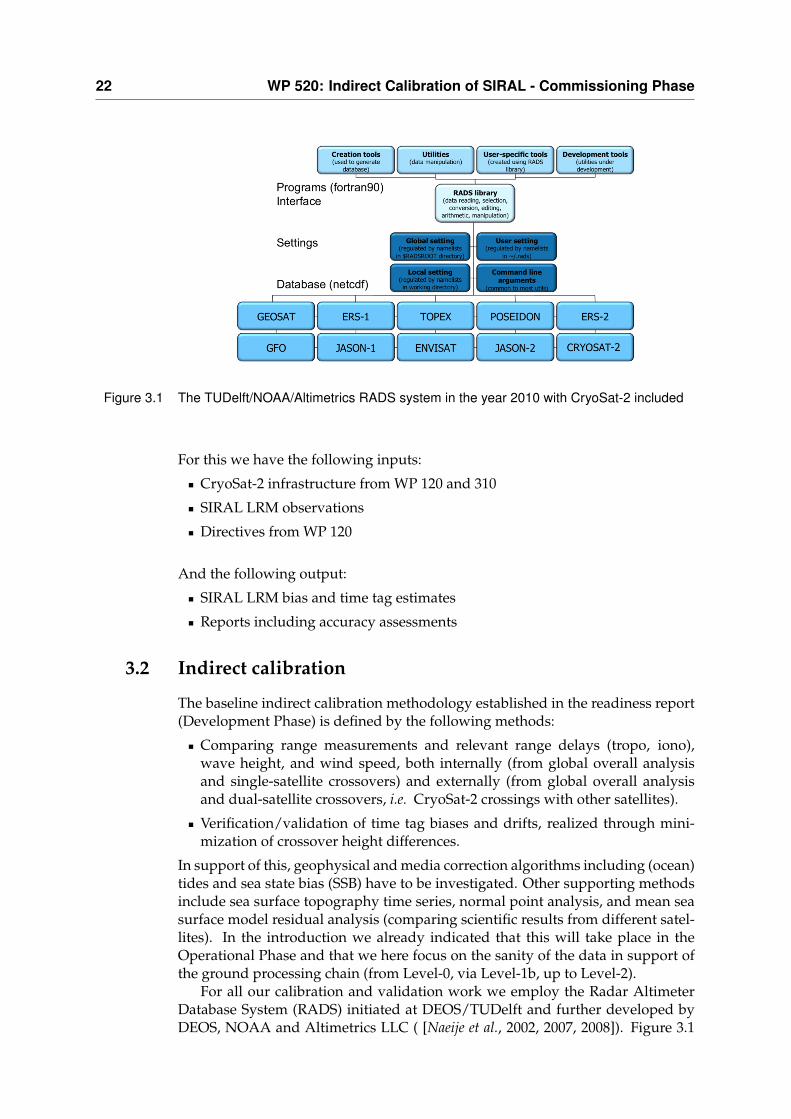
Figure 3.1 The TUDelft/NOAA/Altimetrics RADS system in the year 2010 with CryoSat-2 included

For this we have the following inputs:

CryoSat-2 infrastructure from WP 120 and 310

SIRAL LRM observations

Directives from WP 120

And the following output:

SIRAL LRM bias and time tag estimates

Reports including accuracy assessments

3.2 Indirect calibration

The baseline indirect calibration methodology established in the readiness report(Development Phase) is defined by the following methods:

Comparing range measurements and relevant range delays (tropo, iono),wave height, and wind speed, both internally (from global overall analysisand single-satellite crossovers) and externally (from global overall analysisand dual-satellite crossovers, i.e. CryoSat-2 crossings with other satellites).

Verification/validation of time tag biases and drifts, realized through mini-mization of crossover height differences.

In support of this, geophysical and media correction algorithms including (ocean)tides and sea state bias (SSB) have to be investigated. Other supporting methodsinclude sea surface topography time series, normal point analysis, and mean seasurface model residual analysis (comparing scientific results from different satel-lites). In the introduction we already indicated that this will take place in theOperational Phase and that we here focus on the sanity of the data in support ofthe ground processing chain (from Level-0, via Level-1b, up to Level-2).

For all our calibration and validation work we employ the Radar AltimeterDatabase System (RADS) initiated at DEOS/TUDelft and further developed byDEOS, NOAA and Altimetrics LLC ( [Naeije et al., 2002, 2007, 2008]). Figure 3.1

3.3 Experiences with SIRAL LRM data 23

shows the general concept of RADS. This system not only contains all historicalaltimeter data up to date but also facilitates easy access, cross-calibration and dataanalysis (”system tools”). In 2009 the system was overhauled, software totallyrewritten in Fortran 90 and now storing the data in NETCDF format. The actualwork in frame of our project mainly consisted of transferring and by that con-verting CryoSat-2 LRM Level-2 data to the native RADS (V3) format; the ”SIRALreader” software. To ensure an operational work environment during commis-sioning phase the entire RADS system was ported to a separate multicore XeonTM

server running the SUSE Linux operating system. There is only a limited numberof people that have access to this machine and the incoming data was shieldedfrom other users.

3.3 Experiences with SIRAL LRM data

Purpose of validation is the confirmation that everything in the product is ac-cording to the product specification and within sensible predefined ranges. Cal-ibration on the other hands seeks systematic biases to bring the product closerto reality, e.g. by inter-comparison with data from other missions and/or mod-els. Additionally, we have checked the data against the description in the Level-2products format specification, meaning that all slots in the data records have beenexamined. The check on the orbit parameters is dealt with in more detail in the”precise orbit determination” (POD) work of the project. During the commission-ing phase we came across various errors, bugs, nonconformities and limitationsin the SIRAL LRM level 2 data that we reported to ESA.

We focus our analysis on the time frame 29 August 2010 up to and including29 September 2010, to make sure we use the ”latest” data that already has gonethrough a number of ground track processing revisions during the commission-ing phase, doesn’t suffer from the ionospheric correction bug that was reportedearlier (which affected not just the correction itself but also the actual height mea-surement) and also to have a stretch of data that was not disturbed by large orbitmaneuvers. A 30-day period (referred to as ”September 2010”) was also cho-sen to have one complete subcycle of CryoSat’s orbit. One full cycle is 369 days,which means the exact geographic location is revisited after 369 days, resultingin a 7.5 km track separation at the equator; for a sybcycle this is about 90 km. Wescreened the data for ”open ocean” (surface type flag) and dry tropospheric, wettropospheric and ionospheric correction not equaling zero.

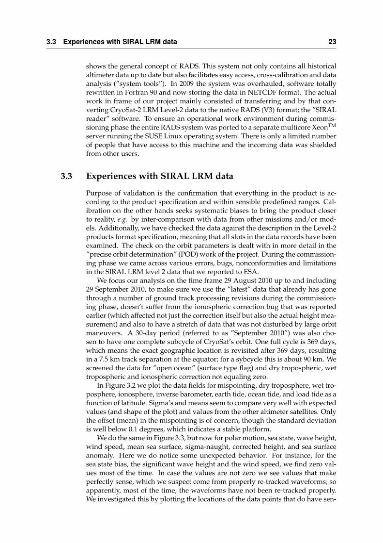
In Figure 3.2 we plot the data fields for mispointing, dry troposphere, wet tro-posphere, ionosphere, inverse barometer, earth tide, ocean tide, and load tide as afunction of latitude. Sigma’s and means seem to compare very well with expectedvalues (and shape of the plot) and values from the other altimeter satellites. Onlythe offset (mean) in the mispointing is of concern, though the standard deviationis well below 0.1 degrees, which indicates a stable platform.

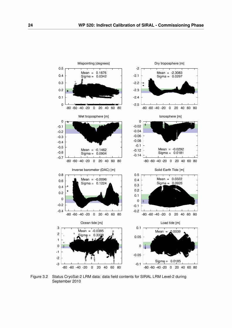
We do the same in Figure 3.3, but now for polar motion, sea state, wave height,wind speed, mean sea surface, sigma-naught, corrected height, and sea surfaceanomaly. Here we do notice some unexpected behavior. For instance, for thesea state bias, the significant wave height and the wind speed, we find zero val-ues most of the time. In case the values are not zero we see values that makeperfectly sense, which we suspect come from properly re-tracked waveforms; soapparently, most of the time, the waveforms have not been re-tracked properly.We investigated this by plotting the locations of the data points that do have sen-


Figure 3.2 Status CryoSat-2 LRM data: data field contents for SIRAL LRM Level-2 duringSeptember 2010

3.3 Experiences with SIRAL LRM data 25

Figure 3.3 Status CryoSat-2 LRM data continued: remaining data field contents for SIRAL LRMLevel-2 during September 2010


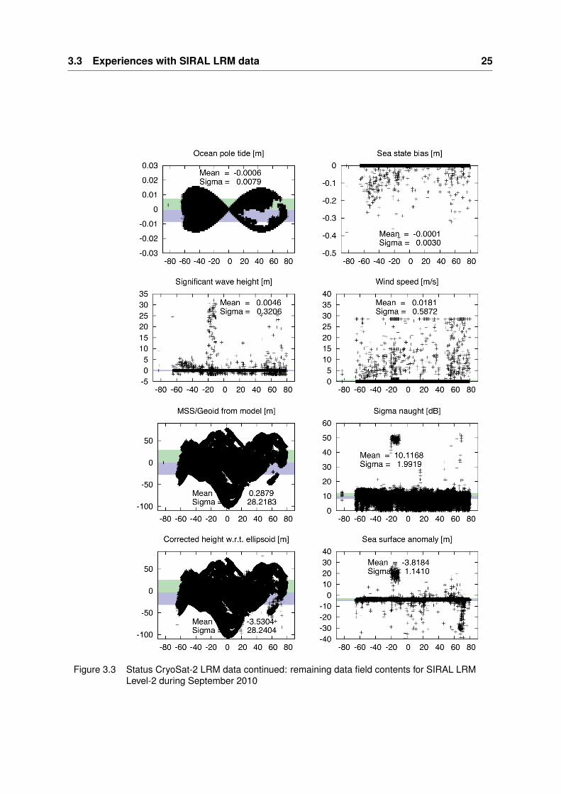
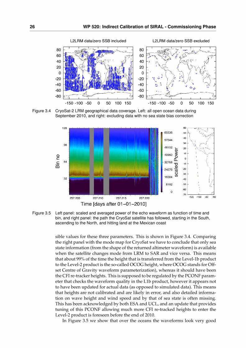
Figure 3.4 CryoSat-2 LRM geographical data coverage. Left: all open ocean data duringSeptember 2010, and right: excluding data with no sea state bias correction

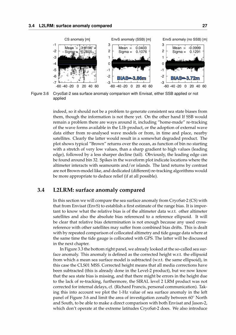
Figure 3.5 Left panel: scaled and averaged power of the echo waveform as function of time andbin, and right panel: the path the CryoSat satellite has followed, starting in the South,ascending to the North, and hitting land at the Mexican coast

sible values for these three parameters. This is shown in Figure 3.4. Comparingthe right panel with the mode map for CryoSat we have to conclude that only seastate information (from the shape of the returned altimeter waveform) is availablewhen the satellite changes mode from LRM to SAR and vice versa. This meansthat about 99% of the time the height that is transferred from the Level-1b productto the Level-2 product is the so-called OCOG height, where OCOG stands for Off-set Centre of Gravity waveform parameterization), whereas it should have beenthe CFI re-tracker heights. This is supposed to be regulated by the PCONF param-eter that checks the waveform quality in the L1b product, however it appears notto have been updated for actual data (as opposed to simulated data). This meansthat heights are not calibrated and are likely in error, and also detailed informa-tion on wave height and wind speed and by that of sea state is often missing.This has been acknowledged by both ESA and UCL, and an update that providestuning of this PCONF allowing much more CFI re-tracked heights to enter theLevel-2 product is foreseen before the end of 2010.

In Figure 3.5 we show that over the oceans the waveforms look very good

3.4 L2LRM: surface anomaly compared 27

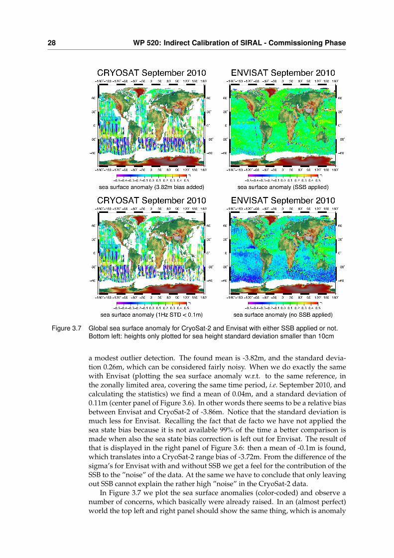
Figure 3.6 CryoSat-2 sea surface anomaly comparison with Envisat, either SSB applied or notapplied

indeed, so it should not be a problem to generate consistent sea state biases fromthem, though the information is not there yet. On the other hand If SSB wouldremain a problem there are ways around it, including ”home-made” re-trackingof the wave forms available in the L1b product, or the adoption of external wavedata either from re-analysed wave models or from, in time and place, nearbysatellites. Clearly the latter would result in a somewhat degraded product. Theplot shows typical ”Brown” returns over the ocean, as function of bin no startingwith a stretch of very low values, than a sharp gradient to high values (leadingedge), followed by a less sharper decline (tail). Obviously, the leading edge canbe found around bin 32. Spikes in the waveform plot indicate locations where thealtimeter interacts with seamounts and/or islands. The land returns by contrastare not Brown-model like, and dedicated (different) re-tracking algorithms wouldbe more appropriate to deduce relief (if at all possible).

3.4 L2LRM: surface anomaly compared

In this section we will compare the sea surface anomaly from CryoSat-2 (CS) withthat from Envisat (EnvS) to establish a first estimate of the range bias. It is impor-tant to know what the relative bias is of the altimeter data w.r.t. other altimetersatellites and also the absolute bias referenced to a reference ellipsoid. It willbe clear that relative bias determination is not enough because any used cross-reference with other satellites may suffer from combined bias drifts. This is dealtwith by repeated comparison of collocated altimetry and tide gauge data where atthe same time the tide gauge is collocated with GPS. The latter will be discussedin the next chapter.

In Figure 3.3 the bottom right panel, we already looked at the so-called sea sur-face anomaly. This anomaly is defined as the corrected height w.r.t. the ellipsoidfrom which a mean sea surface model is subtracted (w.r.t. the same ellipsoid), inthis case the CLS01 MSS. Corrected height means that all media corrections havebeen subtracted (this is already done in the Level-2 product), but we now knowthat the sea state bias is missing, and that there might be errors in the height dueto the lack of re-tracking, furthermore, the SIRAL level 2 LRM product was notcorrected for internal delays, cf. (Richard Francis, personal communication). Tak-ing this into account we plot the 1-Hz value of sea surface anomaly in the leftpanel of Figure 3.6 and limit the area of investigation zonally between 60◦ Northand South, to be able to make a direct comparison with both Envisat and Jason-2,which don’t operate at the extreme latitudes CryoSat-2 does. We also introduce


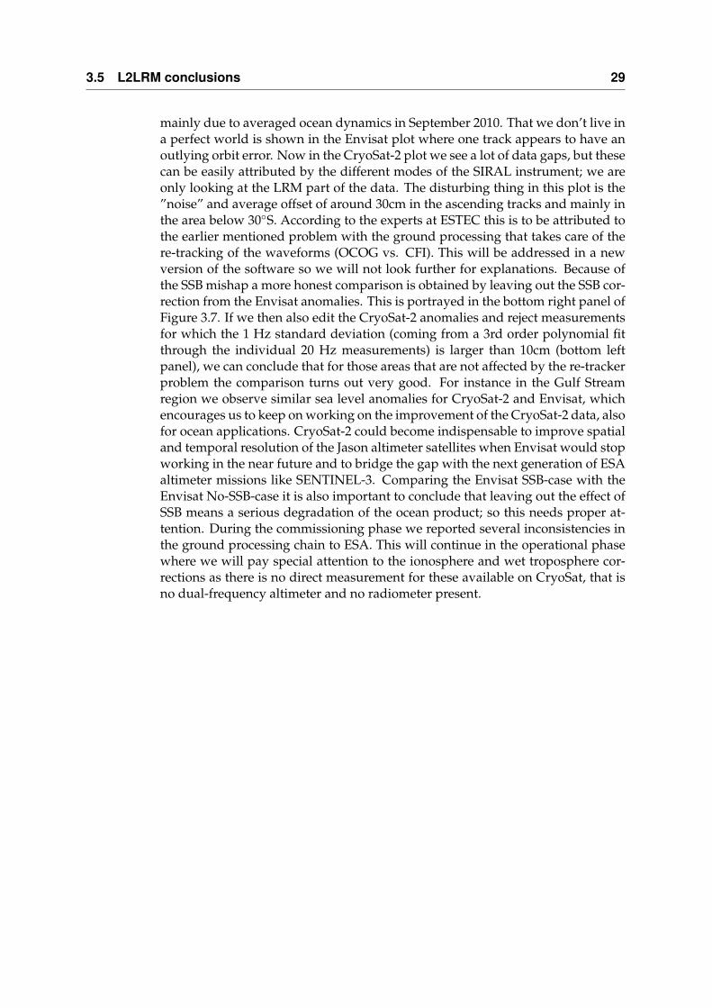
Figure 3.7 Global sea surface anomaly for CryoSat-2 and Envisat with either SSB applied or not.Bottom left: heights only plotted for sea height standard deviation smaller than 10cm

a modest outlier detection. The found mean is -3.82m, and the standard devia-tion 0.26m, which can be considered fairly noisy. When we do exactly the samewith Envisat (plotting the sea surface anomaly w.r.t. to the same reference, inthe zonally limited area, covering the same time period, i.e. September 2010, andcalculating the statistics) we find a mean of 0.04m, and a standard deviation of0.11m (center panel of Figure 3.6). In other words there seems to be a relative biasbetween Envisat and CryoSat-2 of -3.86m. Notice that the standard deviation ismuch less for Envisat. Recalling the fact that de facto we have not applied thesea state bias because it is not available 99% of the time a better comparison ismade when also the sea state bias correction is left out for Envisat. The result ofthat is displayed in the right panel of Figure 3.6: then a mean of -0.1m is found,which translates into a CryoSat-2 range bias of -3.72m. From the difference of thesigma’s for Envisat with and without SSB we get a feel for the contribution of theSSB to the ”noise” of the data. At the same we have to conclude that only leavingout SSB cannot explain the rather high ”noise” in the CryoSat-2 data.

In Figure 3.7 we plot the sea surface anomalies (color-coded) and observe anumber of concerns, which basically were already raised. In an (almost perfect)world the top left and right panel should show the same thing, which is anomaly

3.5 L2LRM conclusions 29

mainly due to averaged ocean dynamics in September 2010. That we don’t live ina perfect world is shown in the Envisat plot where one track appears to have anoutlying orbit error. Now in the CryoSat-2 plot we see a lot of data gaps, but thesecan be easily attributed by the different modes of the SIRAL instrument; we areonly looking at the LRM part of the data. The disturbing thing in this plot is the”noise” and average offset of around 30cm in the ascending tracks and mainly inthe area below 30◦S. According to the experts at ESTEC this is to be attributed tothe earlier mentioned problem with the ground processing that takes care of there-tracking of the waveforms (OCOG vs. CFI). This will be addressed in a newversion of the software so we will not look further for explanations. Because ofthe SSB mishap a more honest comparison is obtained by leaving out the SSB cor-rection from the Envisat anomalies. This is portrayed in the bottom right panel ofFigure 3.7. If we then also edit the CryoSat-2 anomalies and reject measurementsfor which the 1 Hz standard deviation (coming from a 3rd order polynomial fitthrough the individual 20 Hz measurements) is larger than 10cm (bottom leftpanel), we can conclude that for those areas that are not affected by the re-trackerproblem the comparison turns out very good. For instance in the Gulf Streamregion we observe similar sea level anomalies for CryoSat-2 and Envisat, whichencourages us to keep on working on the improvement of the CryoSat-2 data, alsofor ocean applications. CryoSat-2 could become indispensable to improve spatialand temporal resolution of the Jason altimeter satellites when Envisat would stopworking in the near future and to bridge the gap with the next generation of ESAaltimeter missions like SENTINEL-3. Comparing the Envisat SSB-case with theEnvisat No-SSB-case it is also important to conclude that leaving out the effect ofSSB means a serious degradation of the ocean product; so this needs proper at-tention. During the commissioning phase we reported several inconsistencies inthe ground processing chain to ESA. This will continue in the operational phasewhere we will pay special attention to the ionosphere and wet troposphere cor-rections as there is no direct measurement for these available on CryoSat, that isno dual-frequency altimeter and no radiometer present.


3.5 L2LRM conclusions

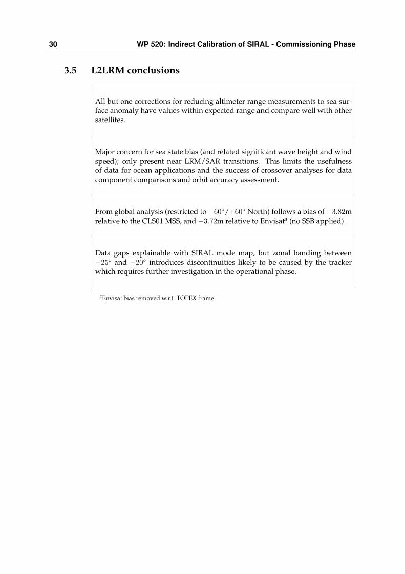
All but one corrections for reducing altimeter range measurements to sea sur-face anomaly have values within expected range and compare well with othersatellites.

Major concern for sea state bias (and related significant wave height and windspeed); only present near LRM/SAR transitions. This limits the usefulnessof data for ocean applications and the success of crossover analyses for datacomponent comparisons and orbit accuracy assessment.

From global analysis (restricted to −60◦/+60◦ North) follows a bias of −3.82mrelative to the CLS01 MSS, and −3.72m relative to Envisata (no SSB applied).

Data gaps explainable with SIRAL mode map, but zonal banding between−25◦ and −20◦ introduces discontinuities likely to be caused by the trackerwhich requires further investigation in the operational phase.

aEnvisat bias removed w.r.t. TOPEX frame

Chapter 4

WP 530: Tide Gauge Calibrationof SIRAL - Commissioning Phase

This section concerns the activities for the (absolute) tide gauge calibration of theSIRAL LRM Level-2 data and provides the status at the end of the Commission-ing Phase. This work, referred to as WP 530 in the ”CryoSat-2 Precise Orbit De-termination and Indirect Calibration of SIRAL” project plan, entailed preparinglogistics for the use of tide gauges in Lake Erie and other parts of the Great Lakesand tide gauges near Hawaii. Subsequently the altimeter data has to be subjectedto the direct comparison with tide gauge data to be able to establish both relativebias and absolute bias. Especially the latter could give insight in possible biasdrifts which would be obscured by drifts in the TOPEX frame when we wouldrestrict ourselves to cross-calibration with other satellites (all unbiased w.r.t. tothe TOPEX frame). The results that are presented here are limited in usefulnessbecause of the data problems mentioned in the previous Chapter. This has beenacknowledged by ESA, and adding to this the importance of a continuous moni-toring of range bias and time tag bias we will continue the tide gauge calibrationactivities in the Operational Phase.

4.1 Work package tasks, inputs and outputs

Tasks defined under WP 530:

Altimeter bias and drift estimate from tide gauges

Orbit centering and monitoring

For this we have the following inputs:

Input from WP 430

Tide gauge data Lake Erie and UHSLC

DEOS orbits from WP 310, and SSALTO orbits

Directives from WP 120

And the following output:

Reports about altimeter drift assessments

Reports about geographical orbit pattern

32 WP 530: Tide Gauge Calibration of SIRAL - Commissioning Phase

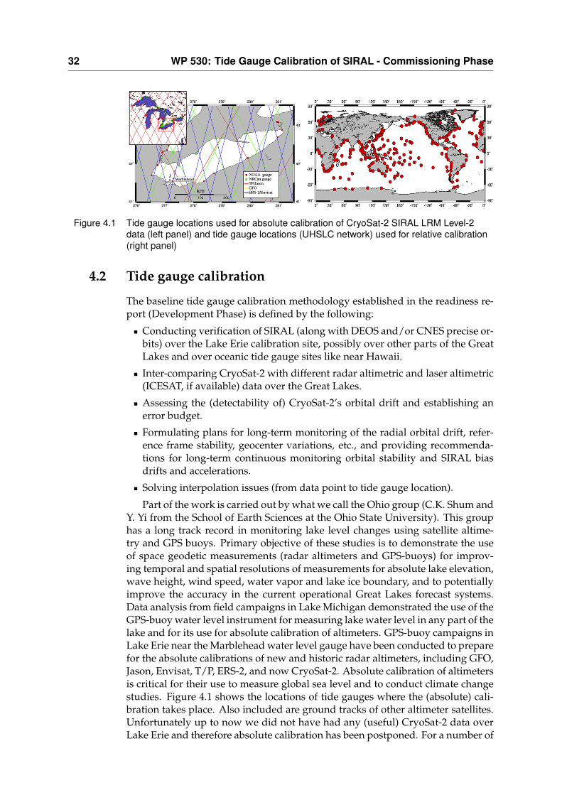
Figure 4.1 Tide gauge locations used for absolute calibration of CryoSat-2 SIRAL LRM Level-2data (left panel) and tide gauge locations (UHSLC network) used for relative calibration(right panel)

4.2 Tide gauge calibration

The baseline tide gauge calibration methodology established in the readiness re-port (Development Phase) is defined by the following:

Conducting verification of SIRAL (along with DEOS and/or CNES precise or-bits) over the Lake Erie calibration site, possibly over other parts of the GreatLakes and over oceanic tide gauge sites like near Hawaii.

Inter-comparing CryoSat-2 with different radar altimetric and laser altimetric(ICESAT, if available) data over the Great Lakes.

Assessing the (detectability of) CryoSat-2’s orbital drift and establishing anerror budget.

Formulating plans for long-term monitoring of the radial orbital drift, refer-ence frame stability, geocenter variations, etc., and providing recommenda-tions for long-term continuous monitoring orbital stability and SIRAL biasdrifts and accelerations.

Solving interpolation issues (from data point to tide gauge location).

Part of the work is carried out by what we call the Ohio group (C.K. Shum andY. Yi from the School of Earth Sciences at the Ohio State University). This grouphas a long track record in monitoring lake level changes using satellite altime-try and GPS buoys. Primary objective of these studies is to demonstrate the useof space geodetic measurements (radar altimeters and GPS-buoys) for improv-ing temporal and spatial resolutions of measurements for absolute lake elevation,wave height, wind speed, water vapor and lake ice boundary, and to potentiallyimprove the accuracy in the current operational Great Lakes forecast systems.Data analysis from field campaigns in Lake Michigan demonstrated the use of theGPS-buoy water level instrument for measuring lake water level in any part of thelake and for its use for absolute calibration of altimeters. GPS-buoy campaigns inLake Erie near the Marblehead water level gauge have been conducted to preparefor the absolute calibrations of new and historic radar altimeters, including GFO,Jason, Envisat, T/P, ERS-2, and now CryoSat-2. Absolute calibration of altimetersis critical for their use to measure global sea level and to conduct climate changestudies. Figure 4.1 shows the locations of tide gauges where the (absolute) cali-bration takes place. Also included are ground tracks of other altimeter satellites.Unfortunately up to now we did not have had any (useful) CryoSat-2 data overLake Erie and therefore absolute calibration has been postponed. For a number of

4.3 Experiences with relative calibration of SIRAL using tide gauges 33

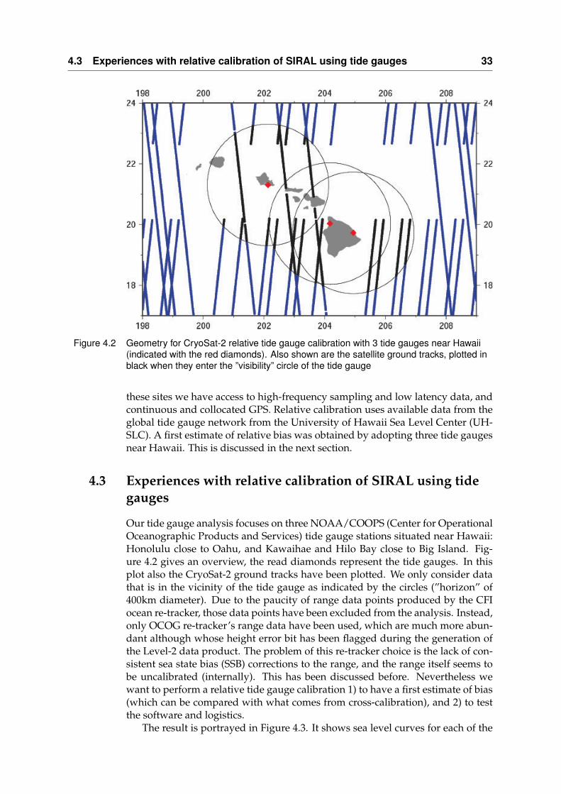
Figure 4.2 Geometry for CryoSat-2 relative tide gauge calibration with 3 tide gauges near Hawaii(indicated with the red diamonds). Also shown are the satellite ground tracks, plotted inblack when they enter the ”visibility” circle of the tide gauge

these sites we have access to high-frequency sampling and low latency data, andcontinuous and collocated GPS. Relative calibration uses available data from theglobal tide gauge network from the University of Hawaii Sea Level Center (UH-SLC). A first estimate of relative bias was obtained by adopting three tide gaugesnear Hawaii. This is discussed in the next section.

4.3 Experiences with relative calibration of SIRAL using tidegauges

Our tide gauge analysis focuses on three NOAA/COOPS (Center for OperationalOceanographic Products and Services) tide gauge stations situated near Hawaii:Honolulu close to Oahu, and Kawaihae and Hilo Bay close to Big Island. Fig-ure 4.2 gives an overview, the read diamonds represent the tide gauges. In thisplot also the CryoSat-2 ground tracks have been plotted. We only consider datathat is in the vicinity of the tide gauge as indicated by the circles (”horizon” of400km diameter). Due to the paucity of range data points produced by the CFIocean re-tracker, those data points have been excluded from the analysis. Instead,only OCOG re-tracker’s range data have been used, which are much more abun-dant although whose height error bit has been flagged during the generation ofthe Level-2 data product. The problem of this re-tracker choice is the lack of con-sistent sea state bias (SSB) corrections to the range, and the range itself seems tobe uncalibrated (internally). This has been discussed before. Nevertheless wewant to perform a relative tide gauge calibration 1) to have a first estimate of bias(which can be compared with what comes from cross-calibration), and 2) to testthe software and logistics.

The result is portrayed in Figure 4.3. It shows sea level curves for each of the

34 WP 530: Tide Gauge Calibration of SIRAL - Commissioning Phase

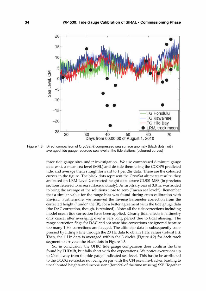
Figure 4.3 Direct comparison of CryoSat-2 compressed sea surface anomaly (black dots) withaveraged tide gauge recorded sea level at the tide stations (coloured curves)

three tide gauge sites under investigation. We use compressed 6-minute gaugedata w.r.t. a mean sea level (MSL) and de-tide them using the COOPS predictedtide, and average them straightforward to 1 per 2hr data. These are the colouredcurves in the figure. The black dots represent the CryoSat altimeter results: theyare based on LRM Level-2 corrected height data above CLS01 MSS (in previoussections referred to as sea surface anomaly). An arbitrary bias of 3.8 m. was addedto bring the average of the solutions close to zero (”mean sea level”). Rememberthat a similar value for the range bias was found during cross-calibration withEnvisat. Furthermore, we removed the Inverse Barometer correction from thecorrected height (”undo” the IB), for a better agreement with the tide gauge data(the DAC correction, though, is retained). Note: all the tide corrections includingmodel ocean tide correction have been applied. Clearly tidal effects in altimetryonly cancel after averaging over a very long period due to tidal aliasing. Therange correction flags for DAC and sea state bias corrections are ignored becausetoo many 1 Hz corrections are flagged. The altimeter data is subsequently com-pressed by fitting a line through the 20 Hz data to obtain 1 Hz values (robust fit).Then, the 1 Hz data is averaged within the 3 circles (Figure 4.2) for each tracksegment to arrive at the black dots in Figure 4.3.

So, in conclusion, the OHIO tide gauge comparison does confirm the biasfound by TUDelft, but falls short with the expectations. We notice excursions upto 20cm away from the tide gauge indicated sea level. This has to be attributedto the OCOG re-tracker not being on par with the CFI ocean re-tracker, leading touncalibrated heights and inconsistent (for 99% of the time missing) SSB. Together

4.4 Tide gauge calibration conclusions 35

with models for the ionospheric correction and wet troposphere correction we arecurrently far away from what would be possible for CryoSat: there is a clear needof validation of data and corrections in the Operational Phase. Knowing thatmost data ”problems” have been addressed, their origin known, and softwarerevisions underway, we are concerned but not worried about CryoSat’s usabilityin ocean applications. As mentioned in the introduction of this chapter we willcontinue the tide gauge assisted calibration in CryoSat’s Operational Phase.

4.4 Tide gauge calibration conclusions

CFI re-tracked corrected height data cannot be used at the moment, becausethey are too few. Inferior OCOG re-tracked corrected height measurements areusable but suffer from SSB problems. This has to be addressed in a new roundof investigations.

CryoSat-2 comparison with tide gauges near Hawaii reveal the same range biasas found by cross-calibration with Envisat, viz. ≈ 3.8m.

CryoSat-2 comparison with tide gauges near Hawaii fall short with expecta-tions and reveal excursions up to 20cm from the tide gauge sea level. Thiscalls for proper validation and calibration of both data and its corrections inthe Operational Phase.

Due to problems with the data, no absolute calibration has been carried out,and also the relative calibration needs revisiting. Here we have to concludethat tide gauge calibration remains important, also in the Operational phase,which we therefore recommend.

Bibliography

ACSL1b (2009), Cryosat ground segment instrument processing facility l1b, (cs-rs-acs-gs–5106), ESA.

ACSL2 (2009), Cryosat ground segment instrument processing facility l2, (cs-rs-acs-gs–5123), ESA.

EADS (2009), Alignment summary document, ESA doc CS-RP-DOR-SY-0055.

ESA (2008), HE-5AS star tracker software interface control document, TER-STR-ICD-001.

Francis, R. (2005), CryoSat reference information, CS-TN-ESA-SY-0441.

Goetz, Christopher (2006), Technical description of the laser retroreflector ar-ray cryosat-lrr-02, issue 1.0, c2-dd-raa-lr-0001 (original id: K01-3095-00-00 to),Federal Unitary State Enterprise - Institute for Precision Instrument.

Naeije, M., R. Scharroo, and E. Doornbos (2007), Next generation altimeter ser-vice: challenges and achievements, in Envisat Symposium, Montreux, Switzer-land, ESA SP-636, edited by H. Lacoste, ESA/ESTEC, 23–27 April 2007.

Naeije, Marc, Eelco Doornbos, Lucy Mathers, Remko Scharroo, Ernst Schrama,and Pieter Visser (2002), Radar altimeter database system: exploitation andextension (radsxx), SRON/NIVR/DEOS publ. NUSP-2 6.3/IS-66 02–06, Nether-lands Agency for Aerospace Programmes (NIVR), Delft, The Netherlands,ISBN 90-5623-077-8.

Naeije, Marc, Remko Scharroo, Eelco Doornbos, and Ernst Schrama (2008),Global altimetry sea-level service: Glass, NUSP-2 report GO 52320 DEO,NIVR/DEOS.

Pavlis DE Poulouse S, McCarthy JJ (2006), Geodyn operations manual, contractorreport, SGI Inc.

Ries, J (2010), ITRF 2005 SLR coordinates, CSR.

Schrama, E., P.N.A.M. Visser, E.N. Doornbos, M.C. Naeije, B.A.C. Ambrosius,C.K. Shum, and A. Braun (2009), Cryosat-2 precise orbit determination andindirect calibration of SIRAL, proposal submitted to ESA in response to con-tract change request no. 001 for CCN-2 ESTEC contract no. 18196/04/NL/GS,DEOS.

Willis, P., J.C. Ries, N.P. Zelensky, L. Soudarin, H. Fagard, E.C. Pavlis, andF.G. Lemoine (2009), DPOD2005 : Realization of a DORIS terrestrial ref-erence frame for precise orbit determination, Advances in Space Research,pp. 44(5):535–544.

Documents

CryoSat-2 Precise Orbit Determination and Indirect ...deos.tudelft.nl/AS/ejo/ejo/text/cs2_cpr_main.pdf · to [email protected], DIODE Navigator and receiver