Culture and Household Saving - Europa

Culture and Household Saving

Benjamin Guin∗

November 2015

Abstract

This paper examines the role of culture in households’ saving decisions. Exploiting the

historical language borders within Switzerland, I isolate the effect of households’ exposure

to certain cultural groups from economic, institutional, demographic and geographic factors

for a homogeneous and representative sample of households. The analysis uses the Swiss

Household Panel which I complement with geographic and socio-economic data. I show that

low- and middle-income households located in the German-speaking part are more than 12

percentage points more likely to save than similar households in the French-speaking part.

I show that these differences across language regions are consistent both with different dis-

tributions of time preferences, and norms of obtaining formal and informal consumer credit

during times of financial distress.

∗Swiss Institute of Banking and Finance, University of St.Gallen (HSG), Switzerland. E-mail: [email protected]. I thank my supervisor Martin Brown for his guidance and support. Moreover, Ithank my conference discussants Steffen Andersen, Mauro Mastrogiacomo and Oscar Stolper for helpfulsuggestions. In addition, I am grateful for comments by Christoph Basten, Marco Di Maggio, BenjaminEnke, Beatrix Eugster, Raymond Fisman, Emilia Garcia-Appendini, Michael Haliassos, Christian Hatten-dorff, Rajkamal Iyer, Raphael Lalive, Michael Lechner, Stephan Meier, Steven Ongena, Thomas Spycher,Johannes Stroebel, Stefan Trautmann and the conference participants of the following conferences: EEA-ESEM 2015 in Mannheim, Netspar Conference in Modena, Western Economic Association Conferencein Wellington, Institutional and Individual Investors: Saving for Old Age Conference in Bath, Congressof the Swiss Society of Economics and Statistics (SSES) in Basel, 8th International Conference of PanelData Users in Lausanne. I also thank the seminar participants at the Austrian National Bank (OeNB) inVienna and University of St.Gallen for helpful comments. This paper uses data from the Swiss HouseholdPanel and I thank Beatrix Eugster and Oliver Lipps for further data enrichments. A first draft of thispaper was written while I was a Chazen Visiting Scholar at Columbia University (GSB); I thank itsbusiness school and Stephan Meier for their hospitality and the Swiss National Science Foundation forfinancial support.

1 Introduction

There are tremendous differences in household saving and accumulated wealth across coun-

tries. Understanding these differences is important, as even small changes in aggregate

savings rates can affect a country’s growth path. In addition, low wealth buffers can im-

peril an economy’s financial stability in the case of adverse income or expenditure shocks.

Typically, economists attempt to explain these differences by economic, institutional, de-

mographic and geographic conditions which vary across countries. As these attempts have

been only partly successful in explaining the observed differences, this paper analyzes the

extent to which exposure to cultural groups can affect households’ intertemporal financial

decisions - in particular their decision to save. Moreover, it considers how culture affects

these decisions.

What is culture and why should it affect households’ intertemporal decisions? Only

recently, economists have transformed the notion of culture from a vague concept by pro-

viding a clear definition that allows for the development of testable empirical predictions.

In line with Guiso et al. (2006) and Fernandez (2011), I define cultural differences as

systematic variation in norms and preferences shared within social groups.

In this paper, I focus on social groups that share a similar language. I argue that

speaking a similar language is a specific dimension of culture and a necessary condition

for any form of social interaction. It enables the transmission of beliefs and preferences

from parents to their children (vertical transmission) or from their peers (horizontal trans-

mission). In line with the existing literature, I test several specific dimensions of norms

and preferences. I argue that different distributions of time preferences and norms of ob-

taining formal or informal consumer credit in financial distress can affect a household’s

decision to save. Impatient households are more likely to consume today than to save for

the future (Sutter et al., 2013). In addition, the norm of mutual help in informal networks

of family and friends in the case of adverse income or expenditure shocks might lead to

lower precautionary saving (Ortigueira and Siassi (2013), Bloch et al. (2008)).

Switzerland is a suitable laboratory to analyze the role of exposure to different lan-

guage groups in households’ intertemporal decisions. In Switzerland, there are two major

language groups: German and French (in addition to Italian and Romansh). The speakers

of these languages are located in separate regions for historical reasons. These regions are

geographically close and share a common language border. At this border, the share of

2

German-speaking individuals falls from 90% to about 20% within 5 kilometers (the share

of French-speaking individuals moves accordingly).

As almost all policies and laws are set either at the national or on the cantonal level,

there is no associated change in policies and institutions at the parts of this border that

run through cantons. In addition, there is no change in geographic conditions, as the

main geographical border, the Alps, runs in an East-West direction, while the language

border separating the German-speaking region from the French-speaking region runs in a

North-South direction. In addition, it is reasonable to assume that economic conditions

that are relevant for households’ saving decisions do not change at the language border

(e.g., business cycles, inflation, interest rates and supply of financial products).

Hence, by comparing the financial decisions of similar households on the German-

speaking side of the language border to those of the households on the French-speaking

side, I am able to isolate the effect of the exposure to these language groups on individual

decisions from institutional, economic and geographic differences. Being able to do this is

important as institutional conditions can affect households’ propensity to save through dif-

ferences in tax incentives (Duflo et al., 2006), pension systems (Borsch-Supan et al., 2008)

and unemployment insurance (Engen and Gruber, 2001). Economic conditions might lead

to different saving behavior in the case of differences in interest rates, inflation (Carroll

and Summers, 1987), business cycles (Carroll et al., 2000) or unemployment expectations

(Basten et al., 2012). Finally, geographic proximity to financial institutions might be rel-

evant to the access and use of financial products (Degryse and Ongena (2005), Agarwal

and Hauswald (2010), Brown et al. (2014)).

To isolate the effect of language group exposure on households’ financial decisions, I

employ survey data from the Swiss Household Panel (waves 1999 until 2012). It includes

characteristics of the person responsible for the management of household finances (“house-

hold head”) (e.g., age, gender, education, etc.), the preferred language spoken (German,

French or Italian) and that person’s religious views. In addition, it contains a wide range

of socio-economic household characteristics, such as income, employment status and the

exact location of each household at the municipality level. Moreover, it includes variables

that have been shown to be good proxies for impatience (e.g., past tobacco consumption)

(e.g., Chabris et al. (2008), Khwaja et al. (2006)). I complement this data set with data

on local unemployment rates at the district level.1

1There are 148 districts in Switzerland (as of January 2013).

3

The empirical strategy is a spatial local border contrast. I test for discontinuities in

household savings at the language border. The key identifying assumption of this local

border contrast is that only the dominant language of each municipality, but no other

pre-determined variable2, changes household saving at the language border. I argue that

this is reasonable to assume - especially for those parts of the language border that run

through cantons, as opposed to those that separate cantons.

I estimate the effect of households’ exposure to language groups on their propensity

to save and to spend excessively. I mainly rely on a variable that indicates whether a

household can save at least CHF 100 per month.3 Alternatively, I employ variables that

indicate whether the household saves voluntarily in a pension fund and whether a house-

hold’s expenditures are higher than its income. To investigate the channels relevant to the

cultural differences in household saving, I complement the main analysis with two further

empirical exercises. First, I test whether different initial distributions of time preferences

are consistent with the observed differences in saving. In particular, I examine whether

households in the German-speaking part are more patient (Channel 1 ). Second, I test

whether households in the French-speaking part are more likely to obtain formal or infor-

mal consumer credit during financial distress. In this case, they should be less likely to

save ex-ante (Channel 2 ).

I document that low- and middle-income households in the German-speaking part are

more than 12 percentage points more likely to save and 6 percentage points less likely to

spend excessively than are similar households in the French-speaking part. These results

are robust, even in terms of more formal testing, when implementing the local border

contrast. I find evidence that there are differences in norms of obtaining credit in financial

distress and impatience that are consistent with the initial differences in household saving

across language regions.

This paper contributes to several strands of the literature. While the role of short-term

social interactions among peers4 has been shown to affect households’ decisions to con-

sume (Kuhn et al. (2011), Angelucci and De Giorgi (2009), Luttmer (2005)), assume debt

(Georgarakos et al., 2014), save for retirement (Duflo and Saez, 2002) and participate in

the stock market (Kaustia and Knupfer (2012), Brown et al. (2008), Hong et al. (2004),

Christelis et al. (2011)), evidence on the role of the long-term vertical dimension of culture

2all variables that are not affected by the dominant language themselves.3CHF 100 is about USD 96 (as of October 2014).4I interpret these as the horizontal dimension of culture.

4

in households’ financial decisions is still scarce.

Existing research has analyzed the role of culture in household debt and portfolios

using cross-country comparisons (e.g., Christelis et al. (2013), Bover et al. (2014), Breuer

and Salzmann (2012)) and examining financial decisions of immigrants to a country (Car-

roll et al. (1994), Haliassos et al. (2014)). While the first strand of the literature faces the

problem of convincingly disentangling country-specific institutional and economic factors

from cultural factors, the second strand faces multiple sample selection issues that arise

when comparing different immigrant groups with one another and with the non-immigrant

population (Bauer and Sinning (2011), Sinning (2011), Piracha and Zhu (2012)). In ad-

dition, in both strands of the literature, it remains unclear which norms and preferences

that are common within cultural groups are relevant to the observed differences in finan-

cial decisions. The present paper overcomes these methodological drawbacks by comparing

the financial decisions of a representative and homogeneous sample of households within

a country. Hereby, I am able to isolate the effect of culture on financial decisions from

differences in institutional, economic and geographic conditions and from differences in

household characteristics.

By examining the channels at work, this paper contributes to the existing literature

on how culture shapes differences in norms and preferences. In particular, the results

of this paper can be interpreted as empirical evidence in favor of the recently developed

linguistic-saving hypothesis. It argues that the future orientation of language can shape

individual time preferences (Chen (2013)). These can, in turn, determine intertemporal

financial decisions. There is evidence in favor of this hypothesis found from controlled lab-

oratory experiments (Sutter et al. (2014)) and cross-country comparisons (Chen, 2013).

The present paper provides evidence for it both within country and for a representative

and homogeneous sample of households.

However, in contrast to Sutter et al. (2014) and Chen (2013), I do not claim that it is

language syntax that shapes time preferences. Instead, I consider the exposure to a certain

language group merely as a necessary condition for the transmission of preferences and

beliefs. Hence, any form of preference or norm could be relevant to the observed differ-

ences in household saving. In particular, an alternative strand of the literature argues that

social norms imply non-pecuniary costs of defaulting on loans (e.g. Guiso et al. (2013),

Fay et al. (2002) and Gross and Souleles (2002)). This paper contributes to this strand

of literature by showing that there are substantial differences in how households resolve

financial distress across cultural groups. These differences are likely to be consistent with

5

non-pecuniary costs, such as the social stigma of obtaining consumer credit in financial

distress.

The remainder of the paper is organized as follows: Section 2 discusses the theoretical

motivation. Section 3 describes the institutional background to the paper. Section 4

presents the data and methodology. Section 5 shows the empirical results of the role

of culture for household saving. Section 6 examines the competing channels of culture.

Section 7 discusses the validity of the results and section 8 draws final conclusions.

6

2 Theoretical Motivation

In this section, I motivate how different distributions of time preferences and norms of

taking credit in financial distress can affect a household’s saving decision. I assume that a

household is faced with the possibility of an uncertain adverse income shock. The house-

hold can insure itself ex-ante (before the income shock materializes) by implementing

precautionary savings. It can be shown it saves more ex-ante, the more patient5 it is

(Channel 1 ). Moreover, a household will not save ex-ante if it takes credit to cover the

income shock once it materializes (Channel 2 ).

In this framework, I assume that a household lives for three periods.

• In period 1, the household earns exogenous income Y1 = Y . It can save a portion of

this income S1 ∈ [0, Y1]. It spends the remaining income on the consumption of a

non-durable good C1 = Y1 − S1.

• In period 2, the household gets back its initial saving S1 (for simplicity I assume

that the interest rate is zero) and earns income Y2. With probability 1 − π it does

not receive an adverse income shock and earns income Y2 = Y . With probability

π the household receives an adverse income shock of σ < Y and earns income of

Y2 = Y − σ. In period 2, the household spends its entire wealth on the consumption

of a non-durable good.

• In period 3, the household receives retirement income of Y3 = Y .

I assume that the household discounts consumption of each subsequent period with a

discount factor of 0 < β ≤ 1.6 Furthermore, I assume that there are two types of house-

holds depending on whether they use credit T in case the shock materializes. Type A

household does not use credit in period 2. Type B household does have access to credit.

In case of a negative income shock, it receives a transfer payment of T = σ, which it repays

in period 3.7

In the first period, the household decides on its initial saving S1 without knowing about

its second-period income Y2. In the following section, I discuss how this saving decision

5Households with higher discount factors.6Note that the discount factor β relates to the discount rate ρ as follows: β ≡ 1

1+ρ . A high discountfactor implies patience.

7I again assume that interest rate is zero. Hence, this household weakly prefers obtaining credit as0 < β ≤ 1.

7

depends on the individual discount factor β and the type of the household.

To obtain a closed-form solution, I make the following assumptions: First, I assume

that utility follows a logarithmic form such that the precautionary saving motive is pre-

served (e.g., Kimball (1990)). Second, I normalize income to one (Y = 1). Third, I

assume that negative income shocks occur with probability π = 12

and are of magnitude

σ = 12Y = 1

2.

In period 1, the household decides on its optimal amount of precautionary saving.

Hereby, it maximizes the expected utility of its lifetime (depending on its anticipated

borrowing in period 2):

maxS1

U(C1) + π β [U(C2L) + β U(C3L)] + (1− π) β [U(C2H) + β U(C3H)] (1)

s.t. C1 = Y1 − S1 = 1− S1 (2)

C2L = Y2 + S1 − σ + T =1

2+ S1 + T (3)

C3L = Y3 − T = 1− T (4)

C2H = Y2 + S1 = 1 + S1 (5)

C3H = Y3 = 1 (6)

It is straightforward to see that the following first-order condition has to hold:

FOC : − 1

1− S1

+ πβ1

12

+ S1 + T+ (1− π)β

1

1 + S1

= 0 (7)

In the following paragraphs, I briefly discuss the saving decisions of both households types.

Type A Household: No credit to cover income shock (T = 0)

First, I consider the case of the household that does not use credit to cover the adverse

income shock. Solving equation 7 for S1, it can be shown that its optimal saving S∗1,A is

strictly positive if its discount factor β is sufficiently high (see Appendix A.1 for details).

S∗1,A > 0, ∀β ∈ (2

3, 1] (8)

This implies that a household that does not take credit will always save ex-ante, if it is

sufficiently patient.

8

Moreover, it can be shown this optimal precautionary saving S∗1,A is increasing in the

discount factor β (see Appendix A.2 for details).

∂S∗1,A∂β

> 0, ∀β ∈ (2

3, 1] (9)

This implies that a household will save more the more patient it is (Channel 1 ).

Type B Household: Credit to cover negative income shock (T = σ)

If the household obtains credit once the income shock occurs, it is straightforward to show

that it would not save (see Appendix A.3 for details).

S∗1,B = 0, ∀0 < β ≤ 1 (10)

This implies that households do not save if they obtain credit once income shocks occur.

Hence, they save less than households that would not take credit if income shocks occur

(Channel 2 ).

Discussion

In this theoretical discussion, I assume that interest rates are the same and zero for all

households. Moreover, income risk is essentially the same for all households (independent

of their cultural exposure). This implies, in particular, that the risk of becoming unem-

ployed is similar across all social groups and all households have similar access to social

insurance (e.g., unemployment benefits). Last, I assume that households in the third pe-

riod that are in retirement, neither borrow nor save.

My empirical research design accounts for these prerequisites by considering only house-

holds that are located within a small geographic scope. Hereby, it is reasonable to assume

that interest rate differences do not exist due to arbitrage. Besides, households have the

same access to social insurance and should face similar risk of unemployment.

Besides, in the empirical part I will only consider households that are non-retired (which

should be equivalent to households that live in period 1 or period 2 in this stylized frame-

work).

9

3 Background

3.1 Languages in Switzerland

In Switzerland, there are four official languages: German, French, Italian and Romansh.

According to the Federal Population Census of 2000, 64.1 percent of the resident popula-

tion of Switzerland declared German as their main language, 20.4 percent speak primarily

French, 6.5 percent speak predominantely Italian, 0.5 percent speak primarily Romansh

(and the rest speak predominantly another language).8 In most of the 26 cantons of

Switzerland, there is only one major language. There are seventeen German-speaking

cantons (e.g., Zurich, St.Gallen and Basel), four French-speaking cantons (Geneva, Jura,

Neuchatel and Vaud) and one Italian-speaking canton (Ticino). In addition, there are

several cantons with more than one official language: the cantons of Bern, Valais, and

Fribourg are bilingual (French and German) and Graubunden is officially trilingual (Ger-

man, Romansh, and Italian).

Figure 1 shows the preferred language spoken by the majority of residents of each mu-

nicipality. It can be seen from this figure that the majority of residents in the north-eastern

part of Switzerland speak predominantly German. In the western part of Switzerland, the

majority of people speak French while the majority of the residents in the southern part

speak Italian (in addition to Romansh). These language regions are geographically close

and share common language borders.

At these language borders, the share of German-speaking households changes abruptly.

Figure 2 shows the share of household heads that prefer to speak German in terms of dis-

tance from the language border separating German from French-speaking municipalities.

It can be easily seen from this figure that the share of German-speaking household heads

changes at the border from about 0.90 to 0.20.9

In Switzerland, most policies are set either at the federal or at the cantonal level.10 For

example, cantons have much discretion in setting cantonal income and wealth tax rates.

This is important, as it is not income before taxes but net income that affects household

saving. Similarly, differences in net wealth could affect household saving. In addition, can-

8Source: http://www.bfs.admin.ch/bfs/portal/en/index/themen/01/05/blank/key/sprachen.html, ac-cessed on October 30th, 2014.

9By definition there is no French-speaking municipality on the German side of the language border(and vice versa).

10Source: https://www.admin.ch/gov/en/start/federal-council/political-system-of-switzerland/swiss-federalism.html, accessed on October 17th, 2015.

10

tons set the curricula of primary and secondary schools, hence, literacy and - in particular

- financial literacy levels could vary across cantons. These factors might themselves affect

household saving.

As I intend to isolate cultural factors from differences in institutional, economic, demo-

graphic and geographic conditions, it is crucial that I focus on multilingual cantons which

have the language border running through them. For this reason, I focus my empirical

analysis on the three bilingual cantons (Bern, Fribourg and Valais). In addition, I only

compare households located in the same canton.

3.2 Differences in Household Saving

While households in Switzerland have similar incentives to save a substantial amount of

their income, there is substantial heterogeneity across language regions. Figure 3 shows

household saving rates in Switzerland in terms of language regions in 2011 (these saving

rates are calculated by subtracting all expenses from the entire household income).11 This

figure suggests that households in the German-speaking part save a higher share of their

income (about 13.2 percent) than do households in the French-speaking part (about 10.5

percent).

My empirical analysis uses the Swiss Household Panel, which includes indicators of

whether households can and do save a certain amount. In particular, I analyze whether

households can save at least CHF 100 per month. Figure 4 shows the share of households

that save at least CHF 100 per month by income levels and by language region in the three

bilingual cantons (Bern, Fribourg, Valais) between 1999-2003. Low income households are

in the lowest quartile of the income distribution in Switzerland per year. Middle and

high income households are in the second & third quartile, and the highest quartile of the

income distribution, respectively. This figure illustrates two stylized facts: First, almost

all households in the highest income group save at least CHF 100 per month irrespective

of the language region they are in. This share is substantially lower among low-income

(around 60 percent) and among middle-income households (about 80 percent). Second,

the share of households that save seems to be more than 10 percentage points lower among

11Data are obtained from the Swiss Household Budget Survey, which is conducted across the seven majorregions of Switzerland. About 3’000 households take part each year. They are chosen randomly from therandom sample register of the Federal Statistical Office. The Household Budget Survey is conducted bymeans of telephone interviews and written questionnaires. Source: http://www.bfs.admin.ch, accessed onOctober 17th, 2015.

11

households located in the French-speaking region than among the ones in the German-

speaking region of Switzerland.

In this paper, I investigate these heterogeneities in household saving. I focus on the

subsample of low- and middle-income households and ask whether the observed differences

between households in the French and German-speaking regions can be explained by their

different cultural exposure.

4 Data, Identification, Estimation

4.1 Data

The empirical analysis uses the Swiss Household Panel. It is a longitudinal survey of

households whose members represent the non-institutional population resident in Switzer-

land. It was first conducted in 1999 and consists of two parts. The first part is a household

questionnaire that contains information on the composition of the household (for example,

household size, household income, etc.). In the second part of the survey, each household

member is interviewed individually about his or her personal characteristics (age, gender,

education, etc.) and whether he or she is responsible for the household finances. For

each household, I only consider the person that is responsible for the household financial

management (“household head”) and match his/her responses to the information about

the household he/she lives in. The survey was conducted by telephone interviews. The

household interviews typically lasted 15 minutes (compared to about 35 minutes required

for the individual interviews).

Financial decisions and household characteristics

The main dependent variable in my empirical analysis is Saving, which indicates whether

the household can save at least CHF 100 monthly. As shown in Table 1, about 83 percent

of my representative sample of low- and middle-income households save at least CHF 100

monthly - which implies that about one-fifth of the households do not save a minimum

share of their income.

The share of non-savers is even higher when analyzing which households save into a retire-

ment savings account. As an alternative dependent variable, I employ Saving (3rd pillar),

which indicates whether the household saves into a “pillar 3” pension fund. It turns out

that the share of households without such an account is more than one-third (Table 1).

Finally, I employ the variable Overspending, which indicates whether the household’s ex-

penses are higher than its income. As indicated in Table 1, about 8 percent of households

12

spend more than they earn.

In addition, I employ the variable Payment arrears as a proxy for households’ financial

distress. This variable indicates whether the household has fallen into payment arrears

within the preceding 12 months.12 Table 1 shows that about 11 percent of all households

fall into payment arrears each year.

Language by municipality, language region and distance to the language

border

I complement the household-level data of the Swiss Household Panel with further informa-

tion on the municipality in which the household is located. In particular, I add information

on the dominant language of each municipality. The binary variable Gi,m indicates whether

the majority of citizens in municipality m, in which the household i is located, prefer to

speak German (French otherwise).

Hence, I define a language region as the set of municipalities that have the same dom-

inant language (French or German). Furthermore, I use the location of each municipality

m in which household i is located to calculate the walking distance to the language border

in kilometers as represented by the variable Distancei,m. I provide further details on the

calculation of these variables in Appendix B.

Household covariates

I employ several household and household head covariates in the empirical analysis. House-

hold variables are Household income and Household size. I also use household head vari-

ables that serve as proxies for gender (Male), education (University), employment status

(Employed, Self employed, Unemployed), preferred language spoken (German speaker)13

and other socio-economic characteristics (Age, Swiss).

Unemployment rates

As existing research has shown that unemployment expectations can have an effect on

households’ saving decisions (e.g., Basten et al. (2012)), I also control for regional unem-

ployment rates. Therefore, I have obtained information on regional unemployment rates

by district and year from State Secretariat for Economic Affairs (SECO).

12Definitions of the variables are provided in Table 12. Summary statistics of all variables are providedin Table 1.

13I only observe the choice of the survey language but not the preferred language in daily life.

13

As my preferred dependent variable Saving is only available in the surveys waves

conducted between 1999 and 2003, I only consider survey respondents from this time

period. Additionally, I only include households that have their primary residence in one

of the three bilingual cantons (Bern, Fribourg and Valais). I also only include households

whose household heads are active in the labor market14 and that are in the lowest three

quartiles of the income distribution in Switzerland for each wave of the survey. My final

sample consists of 577 households that represent the non-institutional low- and middle-

income population in the three bilingual cantons (Bern, Fribourg, Valais) between 1999

and 2003.

4.2 Identification

To clarify the parameter of interest, I make use of the Potential Outcomes Framework.

This enables me to define the causal effect before discussing the assignment mechanism

and without specifying functional form and distributional assumptions.15

The N=577 households covered in my sample are indexed by i = 1, ..., N . In the anal-

ysis, the treatment variable, Gi,m, can assume two different values: Gi,m = 1 if household

i is located in a municipality m in which German is the dominant language. Similarly,

Gi,m = 0, if household i is located in a municipality m in which French is the dominant

language. This definition of the treatment variable is mutually exclusive (as there is only

one dominant language). In addition, it is exhaustive as I consider only municipalities

where either French or German is the dominant language.

I am interested in discovering whether and how the exposure to a different dominant

language group affects the intertemporal decisions of households - in particular, their de-

cision to save. In the main analysis, the binary outcome variable Yi,m assumes the value

of one, if the household i can save at least CHF 100 monthly (zero otherwise). Given the

definition of the treatment, there are two potential outcomes: Yi,m(1) denotes the saving

decision that would be made if household i were located in a German-speaking munici-

pality m; and Yi,m(0) denotes the saving decision that would be made if household i were

located in a French-speaking municipality m. When analyzing the channels of how house-

holds’ exposure to certain language groups affects the observed differences in household

saving, the outcome variable Yi,m represents proxies for households’ time preferences and

their willingness to obtain credit in financial distress.

14I exclude households whose household heads are retired.15See Imbens and Wooldridge (2009) for a more detailed discussion.

14

Relating household saving decisions Yi,m to the type of municipality Gi,m can be con-

founded by variables such as interest rates, inflation rates, unemployment risk, and access

to financial services. These might vary even within Switzerland. Not controlling for all

factors might lead to biased point estimates. To overcome this problem, I apply a Local

Border Contrast16 which compares households that live on one side of the language border

to households that are located on the other side. By considering only households that are

located very close to the border, the importance of confounding variables decreases while

differences in culture are preserved.

In order to implement this local border contrast, I define El(Yi,m) as the limit of the

expectation of Yi,m on the French-speaking side of the language border: i.e., El(Yi,m) =

limε→0−E(Yi,m|Distancei,m = ε). Similarly, I define Er(Yi,m) as the limit of the expec-

tation of Yi,m on the German-speaking side of the language border: i.e., Er(Yi,m) =

limε→0+E(Yi,m|Distancei,m = ε). The treatment effect of interest is as follows (Imbens

and Lemieux, 2008):

δ = E[Yi,m(1)− Yi,m(0)|Distancei,m = 0] = Er(Yi,m)− El(Yi,m)

Discussion

The identification of this Local Average Treatment Effect relies on the assumption that

the potential outcome variable is continuous in the running variable Distancei,m. That is,

E(Yi,m(1)|Distancei,m = x) and E(Yi,m(0)|Distancei,m = x), ∀x ≈ 0 (11)

are continuous in x. This assumption means that two households located in two dif-

ferent, but geographically close municipalities (that have the same dominant language)

have essentially the same propensity to save. In particular, it implies that we would not

expect to see an increase in household saving if we moved a household, together with its

French-speaking municipality, right across the nearby language border to the German side

(and vice versa).

This assumption would be violated if, at the language border, there was a change in

not only the dominant language in the municipality, but also in factors that affect house-

16See Hahn et al. (2001) for a detailed discussion.

15

holds saving decisions but are unaffected by the dominant language in the municipality.

In particular, these could be economic conditions such as deposit interest rates, inflation

rates or unemployment rates.17 I argue that this condition has to hold due to arbitrage.

For example, if deposit interest rates were actually higher in the French-speaking part

than in the German-speaking part, then households in the German-speaking part would

start depositing money in banks in the French-speaking part. They would be able to do

this as transaction costs close to the border are negligible. This increase in the supply of

deposits would decrease equilibrium interest rates in the French-speaking part.18

In addition, this assumption would be violated if pre-determined household covariates

that affect household saving changed discontinuously at the language border (for example,

gender of the household head). However, it does not imply that all household covariates

have to be similar at the border. Instead, I expect some household covariates to be en-

dogenous to the exposure to the dominant language. If, for example, time preferences

actually differed across language regions, then we would expect different education and

employment choices. Different savings rates could translate into different wealth levels

over time.

4.3 Estimation

I estimate this effect using the following linear parametric specification.19

Yi,m = α + δGi,m + βl1Distancei,m + βr1Gi,mDistancei,m +X ′i,mγ + εi,m (12)

where Gi,m is a binary variable that takes on the value of 1 if the majority of the

municipality in which the household i is located speaks German (zero otherwise). Xi,m is

a vector of variables that captures differences between households and municipalities and

contains socio-economic household characteristics. Moreover, this vector contains canton

fixed effects. The latter are important as they ensure that I compare only households that

are located in the same canton. I consider different linear (and non-linear) spatial trends

using the Distancei,m variable. Here, the parameter βl1 estimates the linear spatial trend

in the outcome variable. Similarly, βr1 measures the linear spatial trend in the outcome

variable on the German-speaking side of the language border that is different from the

trend on the French side. Since E[Yi,m|Distancei,m = 0, Gi,m = 1] = α + δ + X ′iγ and

E[Yi,m|Distancei,m = 0, Gi,m = 0] = α+X ′iγ, the parameter of interest is the estimate of δ.

17It is important to understand that this assumption does allow for differences between distant partsof the two language regions but not for differences across language regions close to the border.

18Similar arguments can be made for unemployment rates or inflation rates.19Similar to that used by Eugster et al. (2011).

16

Given the relatively low number of survey respondents that are located in the three

bilingual cantons in my sample, I estimate equation 12 including only the households

that are located within 50 kilometers of the language border (similar to the procedure by

Eugster et al. (2011)). In unreported robustness checks, I show that the results are robust

when varying this ad-hoc bandwidth within a range of 30km to 70km.

I estimate this linear regression using ordinary least squares while clustering the standard

errors on the municipality level. In robustness checks, I show that the effects are robust

to nonlinear estimation.20

5 Language Region and Household Saving

5.1 Household Characteristics & Decisions by Language Region

In this section, I document that the low-and middle-income households located in the

German-speaking part are more likely to save and are less likely to spend more than they

earn. Besides, I show that the households that I consider in my sample are similar in

terms of the household characteristics relevant for the individual saving decision.

Panel A of Table 2 presents a univariate analysis comparing the individual saving de-

cisions of non-retired low- and middle-income households located in the German-speaking

part of Switzerland to the ones located in the French-speaking region. It only considers

households located within 50 km of the language border in the three bilingual cantons

(Bern, Fribourg, Valais) between 1999 and 2003. The table shows that the propensity to

save at least CHF 100 is about 12 percentage points higher among households located

in the German-speaking part (88 percent) than among households in the French-speaking

part (76 percent). This difference is statistically significant at all conventional significance

levels. It is qualitatively similar when considering the share of households that saves ex-

plicitly into a “pillar 3” pension fund (differences of 11 percentage points). In addition,

households in the French-speaking part seem to be about 6 percentage points more likely

to spend more than they earn.

While the households I consider in the sample differ with respect to their intertempo-

ral financial decisions, they are similar in terms of other major dimensions. Panel B of

Table 2 shows that there are no differences in Household income or Household size. Fur-

thermore, the household heads differ not at all or only marginally with respect to major

20I use a Probit estimation reporting marginal effects. The results are available upon request.

17

socio-economic characteristics (Male, University, Age, Swiss, Employed, Self employed,

Unemployed).

5.2 Local Border Contrast: Household Saving

In this section, I show that the univariate differences in household saving are robust to

more rigorous empirical testing. Figure 5 illustrates the share of households that can save

at least CHF 100 per month in terms of their distance from the language border. First,

it can be seen that the share of households that save more than CHF 100 is substantially

lower in the French-speaking part than in the German-speaking part. Second, there is

evidence that the share of households that save at least CHF 100 jumps discontinuously

at the language border, where the walking distance is zero.

I am interested in whether the size of this discontinuity in household saving at the lan-

guage border is economically meaningful and statistically different from zero. Therefore,

I implement the regression in equation 12 and report the point estimate of the parameter

δ. This estimate can be interpreted as the effect of a change in the language region on

households’ saving behavior at the language border.

Table 3 reports my baseline estimates in my preferred sample of non-retired low- and

middle-income households located within 50 km of the language border in the three bilin-

gual cantons (Bern, Fribourg, Valais). The first column shows that the effect of language

region on household saving is about 12 percentage points (without controlling for spatial

trends or any household or regional characteristics). When controlling for linear spatial

trends, canton fixed effects and year fixed effects, this gap increases to 29 percentage points

(column 2). The magnitude and statistical significance remains qualitatively similar af-

ter controlling for socio-economic household characteristics (Household income, Household

size, Male, University, Age, Swiss, Employed, Self employed) and regional unemployment

rates (columns 3 & 5). Moreover, it remains robust to the inclusion of quadratic spatial

trends (columns 4 & 5).21

In unreported robustness checks, I show that these results are robust to decreasing and

increasing the bandwidths by 20 km in both language regions. Moreover, these results are

robust to a non-linear estimation. Besides, the results remain qualitatively similar when

additionally controlling for the main religion of the household head (Catholic, Protestant

or Other). Overall, there is strong empirical evidence that the exposure to certain language

groups affects households’ saving behavior.22

21The results are robust to the inclusion of higher order distance polynomials.22This gap persists when considering households’ decisions to have a “pillar 3” pension fund and to

18

6 Possible Channels

In this paper, I argue that different distributions of time preferences and norms of using

formal or informal consumer credit in financial distress can affect households’ decision to

save. In this section, I explore whether these preferences and norms actually differ across

language regions and whether these differences are consistent with the observed differences

in household saving.

6.1 Channel 1: Time Preferences

Household heads might differ with respect to their individual discount factors. Higher

discount factors imply that households consume less today and shift more wealth to the

future, that is, they save more. It is a natural question to ask whether households in

German-speaking municipalities save more because they have higher discount factors and

are, hence, more patient.

To answer this question, I employ past tobacco consumption as a proxy for individual

impatience and, hence, a discount factor. Several existing studies have shown that there

is a direct relationship between past smoking behavior and individual impatience (e.g.,

Chabris et al. (2008), Khwaja et al. (2006)). The 2010 & 2011 waves of the Swiss House-

hold Panel ask household heads whether they had “ever smoked cigarettes, cigars or a

pipe?”. The binary variable Tobacco smoked takes on the value of one if the household

head responds with “Yes” to this question. In this case, it indicates that the household

head has a low discount factor. If the household head responds with “No” to this question,

the binary variable Tobacco smoked takes on the value of zero. It then indicates that the

household head has a high discount factor.

Again, I test for significant differences in this variable across language regions. As this

variable is only available in the survey waves of 2010 & 2011, I consider households located

within 50 km of the language border in the three bilingual cantons (Bern, Fribourg and

Valais) in these years.

The results in Table 4 show that the percentage of household heads that have ever

smoked tobacco is substantially higher in the French-speaking part (64%) than in the

German-speaking part (55%). The difference of 9 percentage points is economically mean-

ingful and statistically significant at all conventional significance levels. Considering lin-

consume excessively.

19

ear spatial trends (and canton and year fixed effects), the French-German gap increases

in magnitude (to 23 percentage points) and is statistically significant at the five percent

level. The magnitude and statistical significance remains qualitatively similar after con-

trolling for socio-economic household characteristics (Household income, Household size,

Male, University, Age, Swiss, Employed, Self employed) and regional unemployment rates

(columns 3 & 5). Moreover, I find similar results after additionally considering quadratic

spatial trends (columns 4 & 5).

Overall, there is evidence of a discontinuity in my proxy of impatience at the lan-

guage border. In unreported robustness checks, I show that these results are similar when

changing the ad-hoc bandwidths by 20 km and using a non-linear estimation procedure.

6.2 Channel 2: Formal or Informal Credit in Financial Distress

Households face uncertainty regarding future adverse income and expenditure shocks (for

example, due to unemployment, lower bonus payments or unanticipated medical expenses

in case of illness). Ex-ante insurance against these events is often infeasible if insurance

markets are incomplete and do not offer insurance for all contingencies. Besides, ex-ante

insurance might often not be expedient if the insurance premiums offered are not actu-

arially fair. If this is the case, households might conduct higher ex-ante precautionary

savings to accumulate enough wealth that might serve as a buffer against these nega-

tive shocks. Alternatively, households may rely on their informal networks of family and

friends to share the risks of these adverse shocks and smooth consumption. That is, they

may take Informal credit from their networks of family and friends once income shocks

materialize and the household is in financial distress (e.g., Ortigueira and Siassi (2013),

Bloch et al. (2008), Hayashi et al. (1996), Ligon (1998)). Alternatively, these households

might take Formal credit from financial institutions to smooth consumption (e.g., Gertler

et al. (2009)).

In this section, I investigate whether households in the French-speaking part are less

likely to save because they expect to take credit from their informal networks or from

banks when adverse income shocks materialize. I argue that the households I compare in

the empirical analysis are faced with similar conditions on the formal insurance market,

as (i) they are similar in terms of major socio-economic characteristics and (ii) they are

located in geographic proximity within the same canton. Hence, lower savings among

households could be rooted in different norms of taking Formal credit or Informal credit

in financial distress.

20

I suggest an indirect test of this hypothesis by pointing out differences in how house-

holds resolve financial distress. In the survey, the respondents are asked whether they are in

payment arrears and how they resolve such arrears. In particular, they are asked whether

they react to these financial problems “(...) by borrowing from relatives or friends” or

“(...) by borrowing from banks”. In the following analysis, I rely on the binary variable

Informal credit which takes on the value of one, if the household head has borrowed at

least once from family members or friends in case of financial problems (zero otherwise).

Similarly, Formal credit takes on the value of one, if the household head has borrowed at

least once from banks in the time period considered (zero otherwise).

As these questions are asked in each survey wave, I consider all households located

within 50 km of the language border in the three bilingual cantons (Bern, Fribourg, Valais)

over time (1999-2012). Among these households, 308 fell into payment arrears at some

point between 1999 and 2012. In total, there are 740 incidences of financial distress. (This

implies that there are several households that fell into payment arrears more than once).

Table 5 illustrates that there is some evidence that households in the French-speaking

part are more likely to rely on Informal credit once they fall into payment arrears. The

simple mean comparison suggests that these households are on average two percentage

points more likely to take Informal credit. Yet, this difference is not statistically significant

(column 1). When controlling for linear spatial trends (columns 2 & 3) and additionally

controlling for quadratic spatial trends (columns 4 & 5), there is evidence that households

in the French-speaking parts are about 11 - 27 percentage points more likely to take In-

formal credit. Again, these point estimates remain qualitatively similar when decreasing

and increasing the bandwidths by 20 km in both language regions.

In Table 6, I test for differences in relying on Formal credit when falling into payment

arrears. A simple mean comparison reveals that households in the German-speaking part

are about 8 percentage points less likely to take Formal credit than are households in

the French-speaking part (column 1). When linear spatial trends (columns 2 & 3) are

considered and additionally quadratic spatial trends are controlled for (columns 4 & 5),

this difference increases slightly in economic magnitude but remains largely statistically

significant (columns 1, 4 and 5).

I conclude that there are some differences in how households in the French-speaking

part resolve financial distress compared to how households do so in the German-speaking

21

part. There is some evidence that the former are more likely to rely on an informal network

of family and friends once they fall into payment arrears than are the latter. Given that

the households are similar in terms of relevant dimensions and assuming that there are

no differences in the supply of financial products, I interpret this as evidence for higher

risk-sharing among French-speaking households.

In addition, there is also weak evidence that households in the French-speaking part

are more likely to take consumer credit from banks once they fall into payment arrears

than are households in the German-speaking part. A higher degree of risk-sharing and

a higher willingness to take Formal credit might ultimately lead to lower precautionary

saving (e.g., Ortigueira and Siassi (2013)).

7 Robustness & Validity

7.1 Measuring Household Saving and Sample Selection

My preferred outcome variable Saving indicates whether a household can save at least

CHF 100 per month. Using this variable might raise three concerns. First, households

that report that they can save at least CHF 100 do not necessarily actually save. Second,

this binary variable is essentially an arbitrage cutoff point of the distribution of household

saving within Switzerland. Third, this variable only asks for explicit saving of money but

does not take into consideration other forms of saving. In particular, households in the

French-speaking part might be more inclined to put money into housing - for example, by

taking a mortgage to buy a house. In this case, they might have less available income to

save as they have to pay back their mortgage.

In this section, I run several tests to mitigate these concerns. First, I employ two dif-

ferent measures of household saving. I use Saving (3rd pillar) which indicates whether the

household saves into a “pillar 3” pension fund. I also employ the variable Overspending

which indicates whether the household’s expenses are higher than its income. Both vari-

ables ask households not only whether they can save but whether they actually do save.

Panel A and Panel B of Table 7 suggest that there are - indeed - differences in households’

saving behavior across language regions employing these variables. This result should

mitigate concerns that saving behavior might be different at other cutoffs in the saving

distribution and that households’ actual saving behavior might not be appropriately rep-

resented by my preferred saving variable.

22

Furthermore, I repeat my main analysis (as reported in Table 3) but now controlling

for home ownership. If different levels of home ownership were driving the observed differ-

ences in households’ saving behavior, then controlling for it should lower the statistical and

economic significance of the point estimate of the variable German-speaking part. Panel A

of Table 8, however, shows that this is not the case. The point estimates stay statistically

significant and similar in magnitude.

Last, I mitigate concerns that arise due to the selection of my sample. I explicitly con-

sidered only the low- and middle-income households as almost all high-income households

can save at least CHF 100. To mitigate concerns of data mining, I run a robustness test

on the full sample of all households. The results reported in Panel B of Table 8 suggest

that the point estimates of the language region remain robust when considering the full

sample of all households.

7.2 Validity of the Research Design

For robustness, I run a battery of tests that verify the validity of my research design (as

suggested by Imbens and Lemieux (2008)). First, I test for differences in household char-

acteristics across language regions. The mean-comparisons presented in Panel B of Table

2 indicate that the households do not differ in terms of most of the observable household

characteristics that could be relevant for the households’ saving decisions. In addition, I

provide a formal test of the discontinuity of all relevant household characteristics at the

language border. As illustrated in Table 9, I do not find evidence for discrete jumps in

most household covariates at the border.

Second, I test whether there are discontinuities in household saving within the same

language region. As suggested by Imbens and Lemieux (2008), I employ two placebo

tests. In each language region, I take the median distance to the border as a alternative

(”placebo”) borders. I then test whether there are discontinuities in household saving at

these borders. As illustrated in Table 10, I do not find evidence for discrete jumps in

household saving when applying these placebo tests.

Third, I analyze the residuals of the main regression shown in column 2 of Table 3.

If households in the French-speaking part differed in unobservable characteristics from

households in the German-speaking part, the residuals of this regression should be sys-

tematically different. Figure 6 shows that this is not the case: The residuals are scattered

randomly around zero on both sides of the language border.

23

Last, I apply an alternative identification strategy. Instead of using the language region

as the treatment variable, I estimate the effect of the preferred language spoken on the

propensity to save. I control for all observable household and regional characteristics that

I believe can determine the individual saving decision and could be correlated with the

language spoken. I find that French-speaking households are about 11 to 12 percentage

points less likely to save at least CHF 100 per month and are 10 to 11 percentage points

more likely to spend more money than they earn (Table 11).

8 Conclusion

In this paper, I analyze the role of culture in households’ intertemporal financial decisions

making. In particular, I examine whether the exposure to specific language groups affects

households’ decision to save or to overspend. In addition, I elicit potential channels of how

the exposure to certain language groups affects these decisions.

Hereby, I exploit within-country variation of historically determined language regions

in Switzerland. I compare the financial decisions of a representative and homogeneous

sample of low- and middle income households, which are similar on major relevant socio-

economic characteristics on the German-speaking side of the language border, to the ones

on the French-speaking side. To do so, I implement a spatial local border contrast design,

through which I am able to isolate cultural differences of a representative sample of the

population from differences in economic (e.g., business cycles, interest rates and inflation),

institutional (e.g., pension systems, education) and other conditions (e.g., access to finan-

cial services).

The analysis is based on data from the Swiss Household Panel. This survey includes

a wide range of socio-economic household characteristics such as income, the employment

status and the exact location of each household. Furthermore, it includes characteristics of

the person responsible for the management of household finances (“household head”) (in

particular age, gender, and education), the preferred language spoken (French, Italian or

German) and variables that have been shown to be good proxies for time preferences (for

example, past tobacco consumption). I complement the data with detailed information

on language regions and further geographic information about Switzerland.

I document that households in the German-speaking part are more than 12 percentage

points more likely to save and 6 percentage points less likely to spend excessively. These

24

results are robust in comparison with more formal testing when implementing the local

border contrast. I find evidence that the greater use of formal credit in financial distress,

of informal networks of friends and family, and higher time discount rates among French-

speaking households can explain these differences.

Overall, this empirical evidence suggests that culture can - at least partly - explain

some of the observed differences in saving rates we observe across countries.

25

References

Agarwal, S. and R. Hauswald (2010). Distance and Private Information in Lending. Review

of Financial Studies , 1–32.

Angelucci, M. and G. De Giorgi (2009). Indirect Effects of an Aid Program: How Do

Cash Transfers Affect Ineligibles’ Consumption? American Economic Review 99 (1),

486–508.

Basten, C., A. Fagereng, and K. Telle (2012). Saving and portfolio allocation before and

after job loss. Working Paper (672).

Bauer, T. K. and M. G. Sinning (2011). The savings behavior of temporary and permanent

migrants in Germany. Journal of Population Economics 24, 421–449.

Bloch, F., G. Genicot, and D. Ray (2008). Informal insurance in social networks. Journal

of Economic Theory 143 (1), 36–58.

Borsch-Supan, A., A. Reil-Held, and D. Schunk (2008). Saving incentives, old-age provision

and displacement effects: evidence from the German pension reform. Journal of Pension

Economics and Finance 7, 295–319.

Bover, O., J. M. Casado, S. Costa, P. D. Caju, Y. McCarthy, E. Sierminska,

P. Tzamourani, E. Villanueva, and T. Zavadil (2014). The distribution of debt across

euro area countries: the role of individual characteristics, institutions and credit condi-

tions. Deutsche Bundesbank Discussion Paper (1).

Breuer, W. and A. J. Salzmann (2012). National Culture and Household Finance. Global

Economy and Finance Journal (5).

Brown, J. R., Z. Ivkovic, P. A. Smith, and S. Weisbenner (2008). Neighbors Matter: Causal

Community Effects and Stock Market Participation. Journal of Finance LXIII (3),

1509–1531.

Brown, M., B. Guin, and S. Morkotter (2014). Deposit Withdrawals from Distressed

Commercial Banks. Working Paper.

Carroll, C., J. Overland, and D. N. Weil (2000). Saving and Growth with Habit Formation.

American Economic Review 90 (3), 341–355.

Carroll, C., B.-K. Rhee, and C. Rhee (1994). Are there cultural effects on saving? Some

cross-sectional evidence. Quarterly Journal of Economics 3, 685–699.

26

Carroll, C. and L. H. Summers (1987). Why Have Private Savings Rates in the United

States and Canada Diverged? Journal of Monetary Economics 20, 249–279.

Chabris, C., D. Laibson, C. Morris, J. Schuldt, and D. Taubinsky (2008). Individual

laboratory-measured discount rates predict field behavior. Journal of Risk and Uncer-

tainty 37, 237–269.

Chen, K. (2013). The Effect of Language on Economic Behavior: Evidence from Savings

Rates, Health Behaviors, and Retirement Assets. American Economic Review 103 (2),

690–731.

Christelis, D., M. Ehrmann, and D. Georgarakos (2013). Exploring Differences in House-

hold Debt across Euro Area Countries and the US. Working Paper , 1–38.

Christelis, D., D. Georgarakos, and M. Haliassos (2011). Stockholding: Participation,

location, and spillovers. Journal of Banking and Finance 35, 1918–1930.

Degryse, H. and S. Ongena (2005). Distance, Lending Relationships, and Competition.

Journal of Finance 60 (1), 231–266.

Duflo, E., W. Gale, J. Liebman, P. Orszag, and E. Saez (2006). Saving Incentives for

Low- and Middle-Income Families: Evidence from a Field Experiment with H&R Block.

Quarterly Journal of Economics (November), 1311–1346.

Duflo, E. and E. Saez (2002). Participation and investment decisions in a retirement plan:

the influence of colleagues choices. Journal of Public Economics 85, 121–148.

Engen, E. M. and J. Gruber (2001). Unemployment insurance and precautionary saving.

Journal of Monetary Economics 47, 545–579.

Eugster, B., R. Lalive, A. Steinhauer, and J. Zweimuller (2011). The Demand for Social

Insurance: Does Culture Matter? Economic Journal 121, 413–448.

Fay, S., E. Hurst, and M. White (2002). An Empirical Analysis of Personal Bankruptcy

and Delinquency. American Economic Review 92 (3), 706–718.

Fernandez, R. (2011). Does Culture Matter? (1A ed.), Volume 1. Elsevier.

Georgarakos, D., M. Haliassos, and G. Pasini (2014). Household Debt and Social Interac-

tions. Review of Financial Studies .

Gertler, P., D. Levine, and E. Moretti (2009). Do microfinance programs help families

insure consumption against illness? Health Economics 18 (3), 257–273.

27

Gross, D. and N. Souleles (2002). An Empirical Analysis of Personal Bankruptcy and

Delinquency. Review of Financial Studies 15 (1), 319–347.

Guiso, L., P. Sapienza, and L. Zingales (2006). Does Culture Affect Economic Outcomes?

Journal of Economic Perspectives 20 (2), 23–48.

Guiso, L., P. Sapienza, and L. Zingales (2013). The Determinants of Attitudes toward

Strategic Default on Mortgages. Journal of Finance LXVIII (4), 1473–1515.

Hahn, J., P. Todd, and W. V. der Klaauw (2001). Identification and Estimation of Treat-

ment Effects with a Regression-Discontinuity Design. Econometrica 69 (1), 201–209.

Haliassos, M., T. Jansson, and Y. Karabulut (2014). Incompatible European Partners?

Cultural Predispositions and Household Financial Behavior. Working Paper , 1–65.

Hayashi, F., J. Altonji, and L. Kotlikoff (1996). Risk-Sharing between and within Families.

Econometrica 64 (2), 261–294.

Hong, H., J. D. Kubik, and J. C. Stein (2004). Social Interaction and Stock-Market

Participation. Journal of Finance LIX (1), 137–163.

Imbens, G. M. and T. Lemieux (2008). Regression Discontinuity Designs: A guide to

practice. Journal of Econometrics 142, 615–635.

Imbens, G. M. and J. M. Wooldridge (2009). Recent Developments in the Econometrics

of Program Evaluation. Journal of Economic Literature 47 (1), 5–86.

Kaustia, M. and S. Knupfer (2012). Peer performance and stock market entry. Journal

of Financial Economics 104, 321–338.

Khwaja, A., F. Sloan, and M. Salm (2006). Evidence on preferences and subjective beliefs

of risk takers: The case of smokers. International Journal of Industrial Organization 24,

667–682.

Kimball, M. (1990). Precautionary Savings in the Small and in the Large. Economet-

rica 58 (1), 53–73.

Kuhn, P., P. Kooreman, A. Soetevent, and A. Kapteyn (2011). The Effects of Lottery

Prizes on Winners and Their Neighbors: Evidence from the Dutch Postcode Lottery.

American Economic Review 101, 2226–2247.

Ligon, E. (1998). Risk Sharing and Information in Village Economies. Review of Economic

Studies 65, 847–864.

28

Luttmer, E. F. (2005). Neighbors as Negatives: Relative Earnings and Well-Being. Quar-

terly Journal of Economics 120 (3), 963–1002.

Ortigueira, S. and N. Siassi (2013). How important is intra-household risk sharing for

savings and labor supply? Journal of Monetary Economics 60, 650–666.

Piracha, M. and Y. Zhu (2012). Precautionary savings by natives and immigrants in

Germany. Applied Economics 44 (21), 2767–2776.

Sinning, M. G. (2011). Determinants of savings and remittances: empirical evidence from

immigrants to Germany. Review of Economics of the Household 9 (1), 45–67.

Sutter, M., S. Angerer, D. Glatzle-Rutzler, and P. Lergetporer (2014). The effects of

language on children’s intertemporal choices. Working Paper .

Sutter, M., M. Kocher, D. Glatzle-Rutzler, and S. Trautmann (2013). Impatience and

Uncertainty: Experimental Decisions Predict Adolescents’ Field Behavior. American

Economic Review 103 (1), 510–531.

29

Figure 1: Language regions in Switzerland

This figure shows the main language by municipality in Switzerland. Orange illustrates municipalities

with an Italian-speaking majority, dark navy illustrates municipalities with a German-speaking majority,

and red illustrates municipalities with a French-speaking majority (in 2000).

30

Figure 2: German speakers and distance to the language border

This figure shows the share the share of German-speaking household heads depending on the distance to

the language border. The vertical line indicates the language border as detailed in the text. Dots left of

(right of) the vertical line indicate the share of German-speaking household heads in 10km segments in

the French-speaking part (German-speaking part). Source: Swiss Household Panel (1999-2012).

31

Figure 3: Household saving in terms of language region in Switzerland

This figure shows the saving rates of households in Switzerland in terms of language regions in 2011. The

household saving rate is calculated by subtracting all expenses from the entire household income. Source:

Household Budget Survey (HBS) (2011).

0.00

0.02

0.04

0.06

0.08

0.10

0.12

0.14

French‐speaking part German‐speaking part

32

Figure 4: Household saving by language regions and income in Switzerland

This figure shows the share of households that can save at least CHF 100 per month in terms of income

levels and language regions in the three bilingual cantons (Bern, Fribourg, Valais) in 1999-2003. Low-

income (middle-income, high-income) households are households whose household income is in the lowest

quartile (second and third quartile, highest quartile) of the income distribution in Switzerland per survey

wave. Source: Swiss Household Panel (1999-2003).

0.2

.4.6

.81

Sha

re o

f hou

seho

lds

that

can

sav

e at

leas

t CH

F 1

00

Low income Middle income High income

French-speaking part

German-speaking part

33

Figure 5: Saving in terms of language region

This figure shows the share of households that can save at least CHF 100 per month depending on the

distance to the language border. The vertical line indicates the language border as detailed in the text.

Dots left to (right to) the vertical line indicate the share of households that can save at least CHF 100

per 10km segments in the French-speaking part (German-speaking part). Source: Swiss Household Panel

(1999-2003).

0.2

.4.6

.81

1.2

Sha

re o

f hou

seho

lds

that

can

sav

e at

leas

t CH

F 1

00

-50 -40 -30 -20 -10 0 10 20 30 40 50

Walking distance to language border in km

95% Confidence Interval



34

Figure 6: Residuals in terms of language region

This figure shows the residuals of the regression specified in Table 3 Column 2 in the three multilingual

cantons (Bern, Fribourg, Valais) depending on the distance to the language border. The vertical line

indicates the language border as detailed in the text. Dots left to (right to) the vertical line indicate

average residuals per 10km segments in the French-speaking part (German-speaking part). Source: Swiss

Household Panel (1999-2003).

-.8

-.6

-.4

-.2

0.2

.4.6

.8

Res

idua

ls

-50 -40 -30 -20 -10 0 10 20 30 40 50

Walking distance to language border in km

95% Confidence Interval



35

Table 1: Summary statistics

Definitions of the variables are provided in Table 12.

Variable name Mean Std. Dev. Minimum Maximum Observations

Intertemporal Financial DecisionsSaving 0.83 0.38 0.00 1.00 577Saving (3rd pillar) 0.63 0.48 0.00 1.00 577Overspending 0.08 0.26 0.00 1.00 577Homeowner 0.42 0.49 0.00 1.00 577Payment arrears 0.11 0.32 0.00 1.00 6’592

Language variablesGerman-speaking part 0.55 0.50 0.00 1.00 577German speaker 0.55 0.50 0.00 1.00 577Distance 9.17 29.40 -49.09 49.47 577Distance >25km 0.86 0.34 0.00 1.00 577

Socio-economic characteristicsHousehold income 10.46 0.49 8.29 11.13 577Household size 2.81 1.39 1.00 7.00 577Male 0.44 0.50 0.00 1.00 577University 0.14 0.35 0.00 1.00 577Age 40.35 11.82 19.00 68.00 577Swiss 0.91 0.28 0.00 1.00 577Employed 0.77 0.42 0.00 1.00 577Self employed 0.02 0.15 0.00 1.00 577Unemployed 0.02 0.14 0.00 1.00 577

Resolving Payment ArrearsInformal credit 0.36 0.48 0.00 1.00 308Formal credit 0.16 0.36 0.00 1.00 308

Impatience & PlanningTobacco smoked 0.59 0.49 0.00 1.00 508

Regional characteristicsUnemployment 2.22 0.99 0.72 5.20 577

36

Table 2: Household decisions & socio-economic characteristics in terms of language region

This table compares households’ saving and expenses (Panel A) and household and household head char-

acteristics (Panel B) of non-retired low- and middle-income households located in the German-speaking

part of Switzerland to those of the ones located in the French-speaking part of Switzerland between 1999

and 2003. It only considers households located within 50 km of the language border. The last column tests

the differences in means (t-test). The number of household observations (N) is reported in parentheses.

***, **, * denote statistical significance at the 0.01, 0.05 and 0.10-levels, respectively. Definitions of the

variables are provided in Table 12.

Panel A. Households’ financial decisions

German-speakingpart

French-speakingpart Difference

Saving 0.881 0.760 0.121***(N=319) (N=258) (N=577)

Saving (3rd pillar) 0.674 0.566 0.108***(N=319) (N=258) (N=577)

Overspending 0.049 0.109 -0.061***(N=308) (N=247) (N=555)

Panel B. Household and household head characteristics

German-speakingpart

French-speakingpart Difference

Household characteristicsHousehold income 10.485 10.424 0.061

(N=319) (N=258) (N=577)Household size 2.859 2.748 0.111

(N=319) (N=258) (N=577)Household head characteristicsMale 0.458 0.407 0.051

(N=319) (N=258) (N=577)University 0.141 0.147 -0.006

(N=319) (N=258) (N=577)Age 41.179 39.318 1.861*

(N=319) (N=258) (N=577)Swiss 0.925 0.895 0.029

(N=319) (N=258) (N=577)Employed 0.762 0.787 -0.025

(N=319) (N=258) (N=577)Self employed 0.034 0.008 0.027**

(N=319) (N=258) (N=577)Unemployed 0.025 0.016 0.010

(N=319) (N=258) (N=577)

37

Table 3: Household saving in terms of language region

The dependent variable Saving is a binary variable indicating whether the household can save at least CHF

100 per month. German-speaking part is a binary variable indicating whether the household is located

in the German-speaking part of Switzerland (French-speaking part of Switzerland otherwise). Household

control variables are Household income, Household size, Male, University, Age, Swiss, Employed, Self

employed. The regional control variable is the Unemployment rate at the district level. Definitions of the

variables are provided in Table 12. Standard errors are clustered on the municipality level and are reported

in parentheses. ***, **, * denote statistical significance at the 0.01, 0.05 and 0.10-levels, respectively.

1 2 3 4 5

Survey Wave 1999-2003 1999-2003 1999-2003Bandwidth 50km 50km 50km

Dependent variable Saving Saving Saving

German-speaking part 0.121*** 0.294*** 0.359*** 0.280*** 0.355***[0.031] [0.045] [0.061] [0.057] [0.079]

Distance NO Linear Linear Quadratic QuadraticHousehold controls NO NO YES NO YESRegional controls NO NO YES NO YESYear FE NO YES YES YES YESCanton FE NO YES YES YES YES

Observations 577 577 577 577 577Households 577 577 577 577 577Share in German-speaking part 0.55 0.55 0.55 0.55 0.55Municipalities 157 157 157 157 157Mean of dependent variable 0.83 0.83 0.83 0.83 0.83R-squared 0.025 0.048 0.137 0.050 0.137Method OLS OLS OLS OLS OLS

38

Table 4: Time preferences in terms of language region

The dependent variable Tobacco smoked indicates whether the household head has ever smoked tobacco.

German-speaking part is a binary variable indicating whether the household is located in the German-

speaking part of Switzerland (French-speaking part of Switzerland otherwise). Household control variables

are Household income, Household size, Male, University, Age, Swiss, Employed, Self employed. The

regional control variable is the Unemployment rate at the district level. Definitions of the variables

are provided in Table 12. Standard errors are clustered at the municipality level and are reported in

parentheses. ***, **, * denote statistical significance at the 0.01, 0.05 and 0.10-levels, respectively.

1 2 3 4 5

Survey Wave 2010 & 2011 2010 & 2011 2010 & 2011Bandwidth 50km 50km 50km

Dependent variable Tobacco smoked Tobacco smoked Tobacco smoked

German-speaking part -0.091** -0.226** -0.324*** -0.208* -0.256**[0.046] [0.098] [0.107] [0.107] [0.119]

Distance NO Linear Linear Quadratic QuadraticHousehold controls NO NO YES NO YESRegional controls NO NO YES NO YESCanton FE NO YES YES YES YESYear FE NO YES YES YES YES


39

Table 5: Informal credit in financial distress in terms of language region

The dependent variable Informal credit is a binary variable indicating whether the household has borrowed

at least once from family or friends in case of financial distress. German-speaking part is a binary variable

indicating whether the household is located in the German-speaking part of Switzerland (French-speaking

part of Switzerland otherwise). Household control variables are Household income, Household size, Male,

University, Age, Swiss, Employed, Self employed. The regional control variable is the Unemployment rate

at the district level. Definitions of the variables are provided in Table 12. Standard errors are clustered

at the municipality level and are reported in parentheses. ***, **, * denote statistical significance at the

0.01, 0.05 and 0.10-levels, respectively.

1 2 3 4 5


Dependent variable Informal credit Informal credit Informal credit

German-speaking part -0.020 -0.122 -0.111 -0.271*** -0.258**[0.057] [0.094] [0.108] [0.079] [0.108]



40

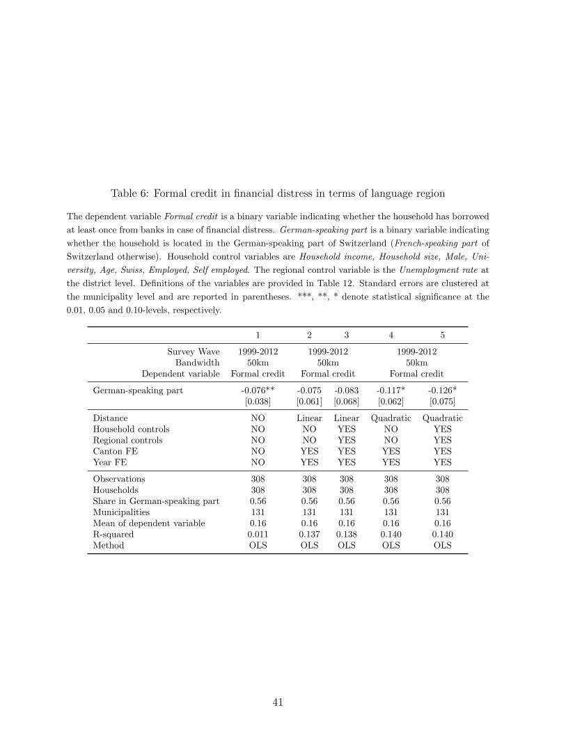
Table 6: Formal credit in financial distress in terms of language region

The dependent variable Formal credit is a binary variable indicating whether the household has borrowed

at least once from banks in case of financial distress. German-speaking part is a binary variable indicating

whether the household is located in the German-speaking part of Switzerland (French-speaking part of

Switzerland otherwise). Household control variables are Household income, Household size, Male, Uni-

versity, Age, Swiss, Employed, Self employed. The regional control variable is the Unemployment rate at

the district level. Definitions of the variables are provided in Table 12. Standard errors are clustered at

the municipality level and are reported in parentheses. ***, **, * denote statistical significance at the

0.01, 0.05 and 0.10-levels, respectively.

1 2 3 4 5


Dependent variable Formal credit Formal credit Formal credit

German-speaking part -0.076** -0.075 -0.083 -0.117* -0.126*[0.038] [0.061] [0.068] [0.062] [0.075]



41

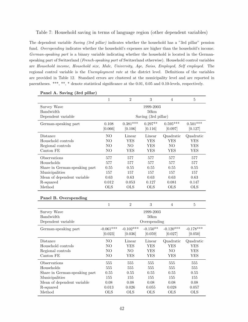
Table 7: Household saving in terms of language region (other dependent variables)

The dependent variable Saving (3rd pillar) indicates whether the household has a ”3rd pillar” pension

fund. Overspending indicates whether the household’s expenses are higher than the household’s income.

German-speaking part is a binary variable indicating whether the household is located in the German-

speaking part of Switzerland (French-speaking part of Switzerland otherwise). Household control variables

are Household income, Household size, Male, University, Age, Swiss, Employed, Self employed. The

regional control variable is the Unemployment rate at the district level. Definitions of the variables

are provided in Table 12. Standard errors are clustered at the municipality level and are reported in

parentheses. ***, **, * denote statistical significance at the 0.01, 0.05 and 0.10-levels, respectively.

Panel A. Saving (3rd pillar)

1 2 3 4 5

Survey Wave 1999-2003Bandwidth 50kmDependent variable Saving (3rd pillar)

German-speaking part 0.108 0.381*** 0.297** 0.595*** 0.501***[0.066] [0.106] [0.116] [0.097] [0.127]

Distance NO Linear Linear Quadratic QuadraticHousehold controls NO YES YES YES YESRegional controls NO NO YES NO YESCanton FE NO YES YES YES YES


Panel B. Overspending

1 2 3 4 5

Survey Wave 1999-2003Bandwidth 50kmDependent variable Overspending

German-speaking part -0.061*** -0.102*** -0.150** -0.120*** -0.178***[0.023] [0.036] [0.059] [0.027] [0.050]



42

Table 8: Household saving in terms of language region (robustness)


100 per month. German-speaking part is a binary variable indicating whether the household is located in

the German-speaking part of Switzerland (French-speaking part of Switzerland otherwise). Homeowner

indicates whether the household owns the property it lives in. Household control variables are Household

income, Household size, Male, University, Age, Swiss, Employed, Self employed. The regional control

variable is the Unemployment rate at the district level. Definitions of the variables are provided in

Table 12. Standard errors are clustered on the municipality level and are reported in parentheses. ***,

**, * denote statistical significance at the 0.01, 0.05 and 0.10-levels, respectively.

Panel A. Saving (controlling for home ownership)

1 2 3 4 5

Survey Wave 1999-2003Bandwidth 50kmDependent variable Saving


Homeowner 0.063* 0.043 0.041 0.041 0.040[0.035] [0.032] [0.032] [0.032] [0.032]



Panel B. Saving (Full sample)

1 2 3 4 5





43

Table 9: Validity: Covariates and language region

The dependent variables are Household income, Household size, Male, University, Age, Swiss, Employed, Self employed. German-speaking part is a

binary variable indicating whether the household is located in the German-speaking part of Switzerland (French-speaking part of Switzerland otherwise).

The regional control variable is the Unemployment rate at the district level. Definitions of the variables are provided in Table 12. Standard errors are

clustered at the municipality level and are reported in parentheses. ***, **, * denote statistical significance at the 0.01, 0.05 and 0.10-levels, respectively.

1 2 3 4 5 6 7 8

Survey Wave 1999-2003Bandwidth 50kmDependent variable Household income Household size Male University Age Swiss Employed Self employed

German-speaking part -0.182 1.211*** 0.181 -0.095 1.429 -0.020 -0.126 0.090[0.138] [0.342] [0.131] [0.103] [2.547] [0.084] [0.122] [0.057]

Distance Quadratic Quadratic Quadratic Quadratic Quadratic Quadratic Quadratic QuadraticHousehold controls NO NO NO NO NO NO NO NORegional controls YES YES YES YES YES YES YES YESCanton FE YES YES YES YES YES YES YES YES

Observations 577 577 577 577 577 577 577 577Households 577 577 577 577 577 577 577 577Share in German-speaking part 0.55 0.55 0.55 0.55 0.55 0.55 0.55 0.55Municipalities 157 157 157 157 157 157 157 157Mean of dependent variable 10.46 2.81 0.44 0.14 40.34 0.91 0.77 0.02R-squared 0.021 0.040 0.006 0.023 0.016 0.011 0.008 0.018Method OLS OLS OLS OLS OLS OLS OLS OLS

44

Table 10: Household saving in terms of language region (robustness)


100 per month. German-speaking part is a binary variable indicating whether the household is located

in the German-speaking part of Switzerland (French-speaking part of Switzerland otherwise). Household

control variables are Household income, Household size, Male, University, Age, Swiss, Employed, Self

employed. The regional control variable is the Unemployment rate at the district level. Definitions of the

variables are provided in Table 12. Standard errors are clustered on the municipality level and are reported

in parentheses. ***, **, * denote statistical significance at the 0.01, 0.05 and 0.10-levels, respectively.

Panel A. Households located in French-speaking part

1 2 3 4


Distance >25km -0.027 -0.018 -0.055 -0.035[0.090] [0.087] [0.099] [0.097]

Distance Linear Linear Quadratic QuadraticHousehold controls NO YES NO YESRegional controls NO YES NO YESCanton FE YES YES YES YES

Observations 258 258 258 258Households 258 258 258 258Share in German-speaking part 0.00 0.00 0.00 0.00Municipalities 73 73 73 73Mean of dependent variable 0.76 0.76 0.76 0.76R-squared 0.043 0.149 0.044 0.149Method OLS OLS OLS OLS

Panel B. Households located in German-speaking part

1 2 3 4


Distance >25km 0.027 0.067 0.168 0.167[0.065] [0.074] [0.113] [0.122]

Distance Linear Linear Quadratic QuadraticHousehold controls NO YES NO YESRegional controls NO YES NO YESCanton FE YES YES YES YES


45

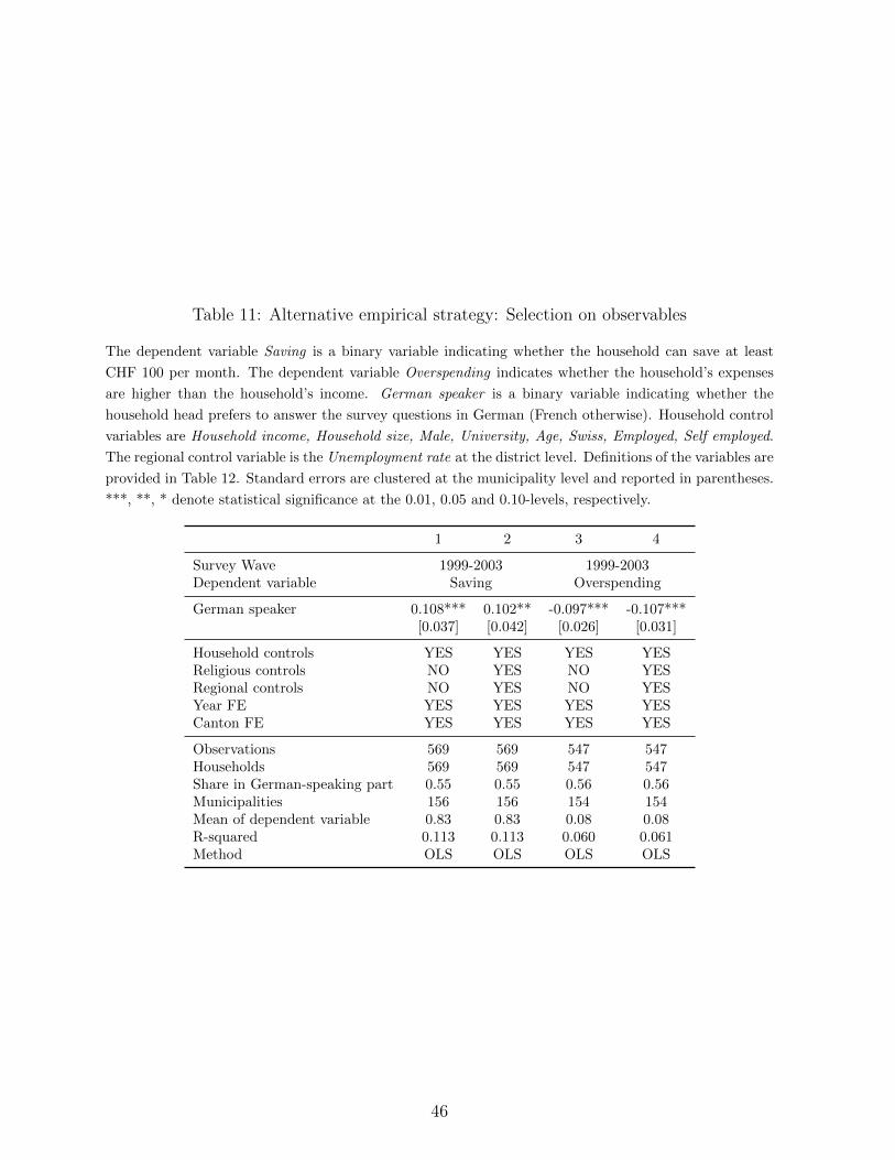
Table 11: Alternative empirical strategy: Selection on observables

The dependent variable Saving is a binary variable indicating whether the household can save at least

CHF 100 per month. The dependent variable Overspending indicates whether the household’s expenses

are higher than the household’s income. German speaker is a binary variable indicating whether the

household head prefers to answer the survey questions in German (French otherwise). Household control

variables are Household income, Household size, Male, University, Age, Swiss, Employed, Self employed.

The regional control variable is the Unemployment rate at the district level. Definitions of the variables are

provided in Table 12. Standard errors are clustered at the municipality level and reported in parentheses.

***, **, * denote statistical significance at the 0.01, 0.05 and 0.10-levels, respectively.

1 2 3 4

Survey Wave 1999-2003 1999-2003Dependent variable Saving Overspending

German speaker 0.108*** 0.102** -0.097*** -0.107***[0.037] [0.042] [0.026] [0.031]

Household controls YES YES YES YESReligious controls NO YES NO YESRegional controls NO YES NO YESYear FE YES YES YES YESCanton FE YES YES YES YES


46

Table 12: Variable definitions

This table provides definitions of variables.

Variable name Definition Source

Intertemporal Financial DecisionsSaving Binary variable = 1 if the household can save at least CHF 100 monthly, = 0 otherwise. SHP 1999 - 2003Saving (3rd pillar) Binary variable = 1 if the household saves into a ”pillar 3” scheme, = 0 otherwise. SHP 1999 - 2003Overspending Binary variable = 1 if the household’s expenses are higher than the household’s income, = 0 otherwise. SHP 1999 - 2003Homeowner Binary variable = 1 if the household owns the property it lives in, = 0 otherwise. SHP 1999 - 2003

Payment arrearsBinary variable = 1 if the household has fallen into payment arrears within the preceding 12 months,

= 0 otherwise. SHP 1999 - 2012

Language variables

German-speaking partBinary variable = 1 if the household is located in the German-speaking part of Switzerland, = 0

if French-speaking part. SHP 1999 - 2003German speaker Binary variable = 1 if the household head prefers to answer the survey questions in German, = 0 if French. SHP 1999 - 2003Distance Walking distance from the language border in km. Search.chDistance >25km Binary variable = 1 if the walking distance from the language border is greater than 25 km, = 0 otherwise. Search.ch

Socio-economic characteristicsHousehold income Net yearly household income in CHF (OECD equivalised) (natural logarithm). SHP 1999 - 2003Household size Number of persons in household SHP 1999 - 2003Male Binary variable = 1 if the household head is male, = 0 otherwise. SHP 1999 - 2003University Binary variable = 1 if the household head holds a unversity degree, = 0 otherwise. SHP 1999 - 2003Age Age of the household head in years. SHP 1999 - 2003Swiss Binary variable = 1 if the household head is Swiss, = 0 otherwise. SHP 1999 - 2003Employed Binary variable = 1 if the household head is employed, = 0 otherwise. SHP 1999 - 2003Self employed Binary variable = 1 if the household head is self employed, = 0 otherwise. SHP 1999 - 2003Unemployed Binary variable = 1 if the household head is unemployed, = 0 otherwise. SHP 1999 - 2003

Resolving Payment Arrears

Informal creditBinary variable = 1 if the household has borrowed at least once from family or friends

in case of financial distress, = 0 otherwise. SHP 1999 - 2012

Formal creditBinary variable = 1 if the household has borrowed at least once from banks

in case of financial distress, = 0 otherwise. SHP 1999 - 2012

Impatience & PlanningTobacco smoked Binary variable = 1 if the household heads have ever smoked tobacco in their lives, = 0 otherwise. SHP 2010; 2011

Regional characteristics

Unemployment

Unemployment rate per district and year (in percent) based on calculation

by State Secretariat for Economic Affairs (SECO). SHP 1999 - 2003

47

A Solution to the Stylized Model

A.1 Type A household (T = 0): Saving decision in t=1

The following first-order condition has to hold:

FOC : − 1

1− S1

+ πβ1

12

+ S1 + T+ (1− π)β

1

1 + S1

= 0 (13)

Assuming that the probability of income shocks is π = 12, this is equivalent to:

2[(1

2+ S1 + T )(1 + S1)] = β(1− S1)[(1 + S1) + (

1

2+ S1 + T )] (14)

Type A household does not obtain credit in distress (T = 0). Plugging in T = 0 in

equation 14, we can solve for the optimal household saving S∗1,A.23

S∗1,A =−3 + 1

2β +

√12.25β2 + β + 1

2(2 + 2β)(15)

Notice that β is non-negative by definition. Hence, the denominator of equation 15 is

positive. Hence, optimal saving of this household type is strictly positive, S∗1,A > 0, if:

√12.25β2 + β + 1 > 3− 1

2β (16)

As 0 < β ≤ 1, it follows from equation 16 that the following inequality has to hold.

=⇒ 12.25β2 + β + 1 > (3− 1

2β)2 (17)

Rearranging terms, we can find the strictly positive solution:

12β2 + 4β − 8 > 0 (18)

Solving for β yields the critical discount factor β∗:24

β∗ >2

3� (19)

23Notice: We are only interested in the solution where S∗1,A ≥ 0.

24Notice: We are only interested in the solution where 0 < β∗ ≤ 1.

48

A.2 Type A household (T = 0): Optimal saving and discount

factor

We want to show that optimal precautionary saving S∗1 is strictly increasing in β, i.e.

∂S∗1,A∂β

> 0,∀2

3< β ≤ 1 (20)

We know from Appendix A.1 that optimal precautionary saving for this household type

is:

S∗1,A =−3 + 1

2β +

√12.25β2 + β + 1

2(2 + 2β)(21)

We check the sign of the first partial derivative with respect to β:

∂S∗1,A∂β

=[12

+ 12a−.5(24.5β + 1)] · (4 + 4β)− [−3 + 1

2β +√a] · 4

(4 + 4β)2(22)

where a ≡ 12.25β2 + β + 1.

Notice that the denominator, (4 + 4β)2, is positive. Hence, the partial derivative∂S∗

1,A

∂β> 0 is positive if:

[1

2+

1

2a−.5(24.5β + 1)] · (4 + 4β)− [−3 +

1

2β +√a] · 4 > 0 (23)

which is equivalent to

[1

2a−.5(24.5β + 1)] · (4 + 4β) + [

1

2(4 + 4β)− [−3 +

1

2β +√a] · 4] +

√2−√

2 > 0 (24)

Inequality 24 is true if the following inequalities 25 and 26 hold true:

1

2a−.5(24.5β + 1) · (4 + 4β) >

√2 (25)

and

1

2· (4 + 4β)− [−3 +

1

2β +√a] · 4 > −

√2 (26)

It is straightforward to show that inequality 25 is true.

⇔ (24.5β + 1) · (2 + 2β) >√

2√a (27)

49

Substituting a ≡ 12.25β2 + β + 1 back in, it is equivalent to.

⇔ 49β2 + 51β + 2 >√

24.5β2 + 2β + 2, ∀0 < β ≤ 1 � (28)

Similarly, one can show that inequality 26 is true. Rearranging terms yields.

⇔ 14− 4√a > −

√2 (29)

which is equivalent to

⇔√a <

14 +√

2

4(30)

Substituting a ≡ 12.25β2 + β + 1 back in.

⇔√

12.25β2 + β + 1 <14 +

√2

4(31)

We can plug in β = 1 in a (as a is strictly increasing in β, for all 0 < β ≤ 1):

√14.25 <

14 +√

2

4, ∀0 < β ≤ 1 � (32)

Hence, optimal precautionary saving S∗1,A is increasing in β. �

50

A.3 Type B household (T = σ): Saving decision in t=1

In case of credit T = σ, the first-order condition (equation 13) simplifies to:

FOC : − 1

1− S1

+ πβ1

1 + S1

+ (1− π)β1

1 + S1

= 0 (33)

Assuming that the probability of income shocks is π = 12, this is equivalent to:

1

1− S1

= β1

1 + S1

(34)

Solving for S1 gives optimal precautionary saving of this household type S∗1,B:

S∗1,B =β − 1

1 + β,∀0 < β ≤ 1 (35)

As∂S∗

1,B

∂β> 0 and S∗1,B < 0,∀0 < β ≤ 1, we conclude that this household type never saves,

i.e. S∗1 = 0 (as saving cannot be negative by definition). �

51

B Data Appendix

In this section, I provide further details on the calculation and sources of the language

variables. These data rely to a large extent on distance data used by Eugster et al. (2011).

B.1 Dominant language per municipality Gi,m

The Swiss Population Census in 2000 conducted by the Federal Statistical Office provides

information on each person’s main language spoken at home. I use this information to

determine the major language of each municipality. The variable Gi,m takes on the value

of one if household i is located in a municipality m where more than 50% of the population

prefer to speak German at home (zero otherwise).25

B.2 Language region

I define a Language region as being the set of municipalities that have the same major lan-

guage. For example, the French-speaking region of Switzerland includes all municipalities

in which the majority of the population prefer speaking French. Similarly, the German-

speaking region of Switzerland includes all municipalities in which the majority of the

population prefer speaking German. This definition is important for the empirical strat-

egy that I point out in section 4. As can be seen in Figure 1, there are several enclaves (i.e.

German-speaking municipalities entirely surrounded by French-speaking municipalities).

In this baseline definition, these German-speaking municipalities are part of the German-

speaking language region. In unreported robustness checks I exclude these enclaves. I can

show that the results remain qualitatively similar.

B.3 Distance to the language border

To calculate the distance to the language border, I use data on the driving distance in

kilometers between any pair of municipalities in Switzerland.26 For each municipality

in the German language region, I define the shortest distance among the distances to

all municipalities in the French language region as being the distance to the language

border. Equivalently, for each French-speaking municipality I take the shortest driving

distance to a municipality in the German-speaking part as being the distance to the

language border. The variable Distancei,m then takes negative values for municipalities

25I rely on year 2000 data assuming that the composition of the language speakers has not changedsubstantially over time.

26The matrix of all distance pairs was obtained from the online platform search.ch.

52

in the French-speaking part and takes positive values for municipalities in the German-

speaking part. The municipalities that serve as the closest municipalities for at least one

municipality on the opposite side of the language border are assigned distance values of

zero (Distancei,m = 0).

53

Documents

Culture and Household Saving - Europa