curs 6.doc

8. THE DISTORTING REGIME(The Non-sinusoidal Permanently Periodic Regime)

8.1 Fourier Analysis

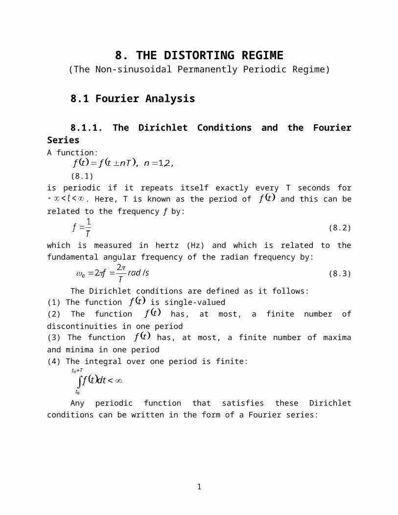
8.1.1. The Dirichlet Conditions and the Fourier SeriesA function:

(8.1)

is periodic if it repeats itself exactly every T seconds for . Here, T is known as the

period of and this can be related to the frequency f by:

(8.2)

which is measured in hertz (Hz) and which is related to the fundamental angular frequency of the

radian frequency by:

(8.3)

The Dirichlet conditions are defined as it follows:

(1) The function is single-valued

(2) The function has, at most, a finite number of discontinuities in one period

(3) The function has, at most, a finite number of maxima and minima in one period

(4) The integral over one period is finite:

Any periodic function that satisfies these Dirichlet conditions can be written in the form

of a Fourier series:

(8.4)

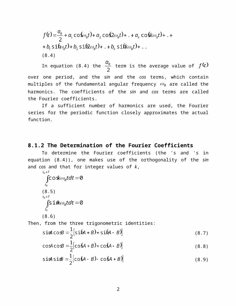
In equation (8.4) the term is the average value of over one period, and the sin and

the cos terms, which contain multiples of the fundamental angular frequency are called the

harmonics. The coefficients of the sin and cos terms are called the Fourier coefficients.

If a sufficient number of harmonics are used, the Fourier series for the periodic function

closely approximates the actual function.

1

8.1.2 The Determination of the Fourier CoefficientsTo determine the Fourier coefficients (the 's and 's in equation (8.4)), one makes use of

the orthogonality of the sin and cos and that for integer values of k,

(8.5)

(8.6)

Then, from the three trigonometric identities:

(8.7)

(8.8)

(8.9)

with and , where k and m are integers, it can be shown that:

(8.10)

(8.11)

(8.12)

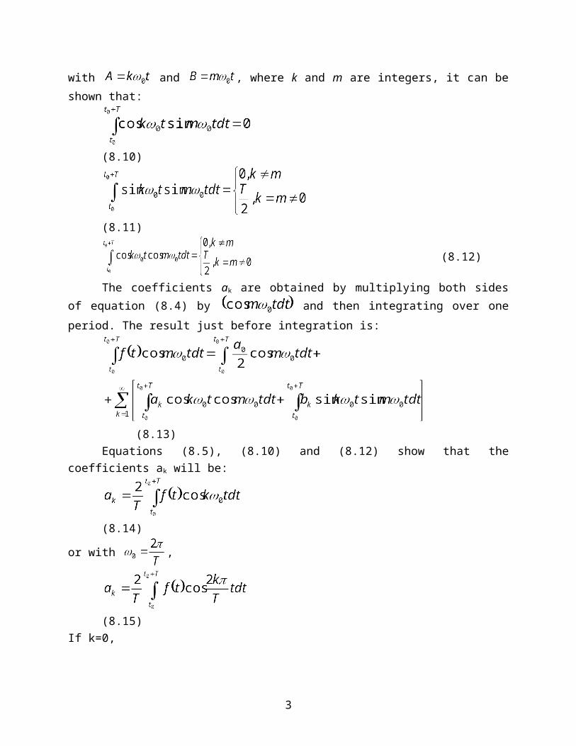
The coefficients ak are obtained by multiplying both sides of equation (8.4) by and then integrating over one period. The result just before integration is:

(8.13)

Equations (8.5), (8.10) and (8.12) show that the coefficients ak will be:

(8.14)

or with ,

2

(8.15)

If k=0,

(8.16)

and it is obvious that use of in equation (8.4) permits the use of a uniform relationship for

finding all of the ak including a0. Moreover, equation (8.16) represents just twice the average

value of over one period.

The bk coefficients are obtained in a similar fashion, but this time equation (8.4) is multiplied by . The form just prior performing the integration is:

(8.17)

Use of equations (8.6), (8.10) and (8.11) show that the coefficients bk will be:

(8.18)

or, if ,

(8.19)

8.1.3 Symmetry considerationsEvaluation of the Fourier coefficients becomes a great deal simpler when certain types of

symmetry are recognized.

Even-Function Symmetry.

An even function is defined by:

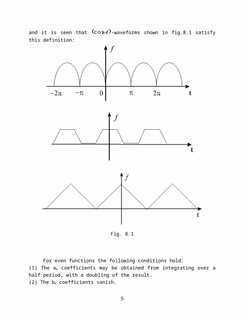
and it is seen that -waveforms shown in fig.8.1 satisfy this definition:

3

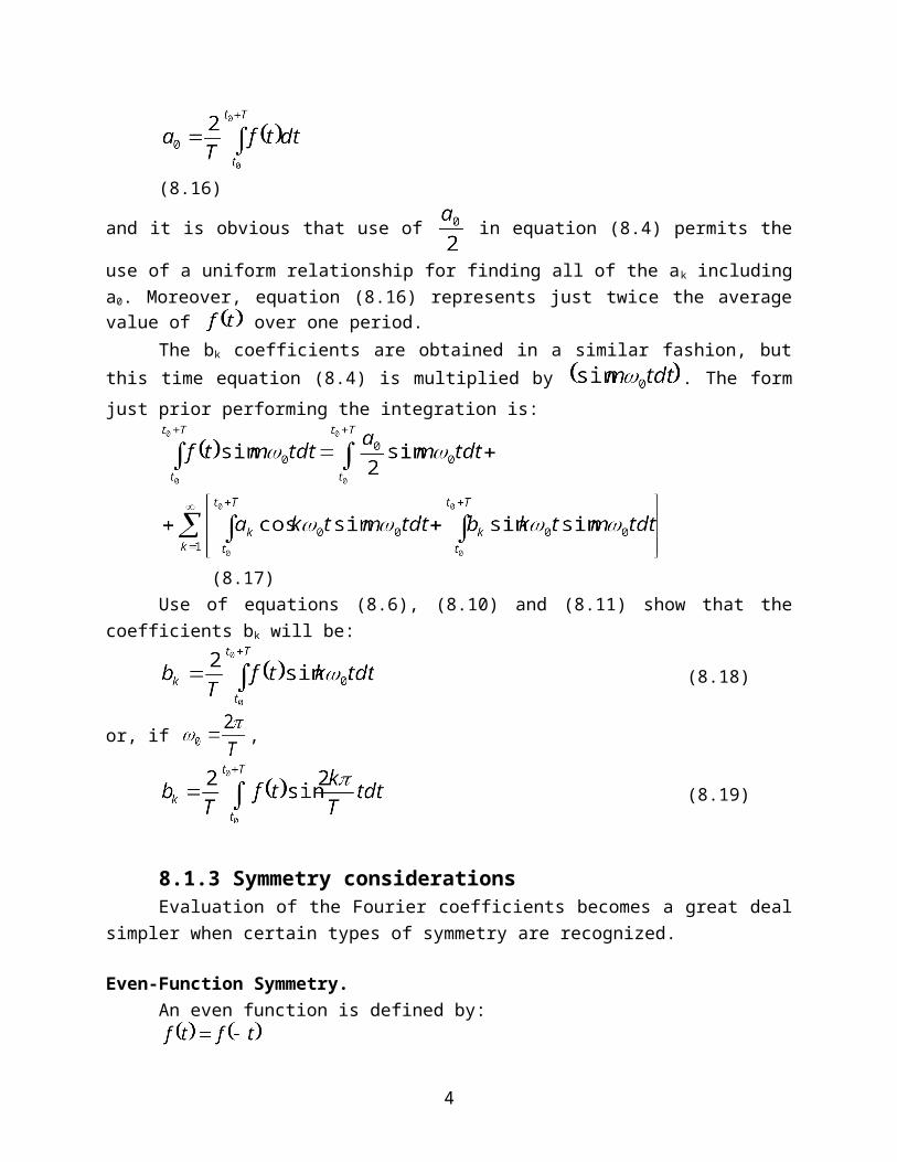
Fig. 8.1

For even functions the following conditions hold:

(1) The ak coefficients may be obtained from integrating over a half period, with a doubling of

the result.

(2) The bk coefficients vanish.

Odd-Function Symmetry.

4

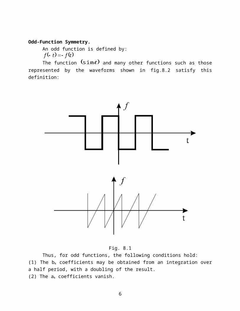
An odd function is defined by:

The function and many other functions such as those represented by the

waveforms shown in fig.8.2 satisfy this definition:

Fig. 8.1

Thus, for odd functions, the following conditions hold:

(1) The bk coefficients may be obtained from an integration over a half period, with a doubling of

the result.

(2) The ak coefficients vanish.

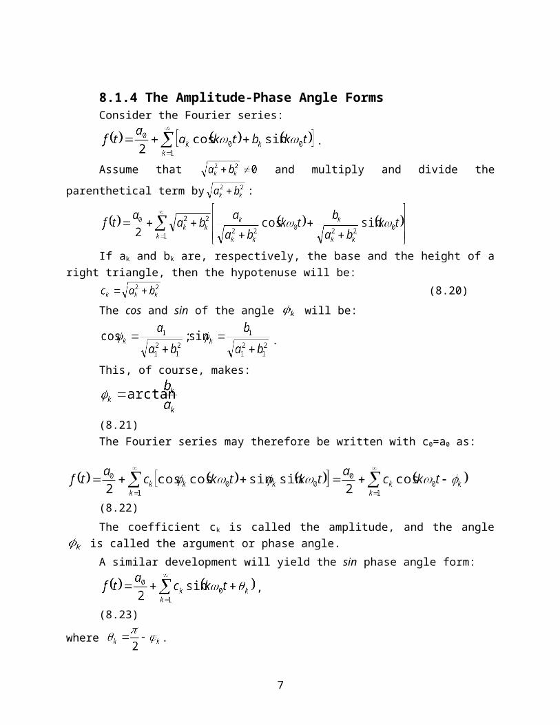
8.1.4 The Amplitude-Phase Angle FormsConsider the Fourier series:

5

.

Assume that and multiply and divide the parenthetical term by :

If ak and bk are, respectively, the base and the height of a right triangle, then the

hypotenuse will be:(8.20)

The cos and sin of the angle will be:

.

This, of course, makes:

(8.21)

The Fourier series may therefore be written with c0=a0 as:

(8.22)

The coefficient ck is called the amplitude, and the angle is called the argument or

phase angle.

A similar development will yield the sin phase angle form:

, (8.23)

where .

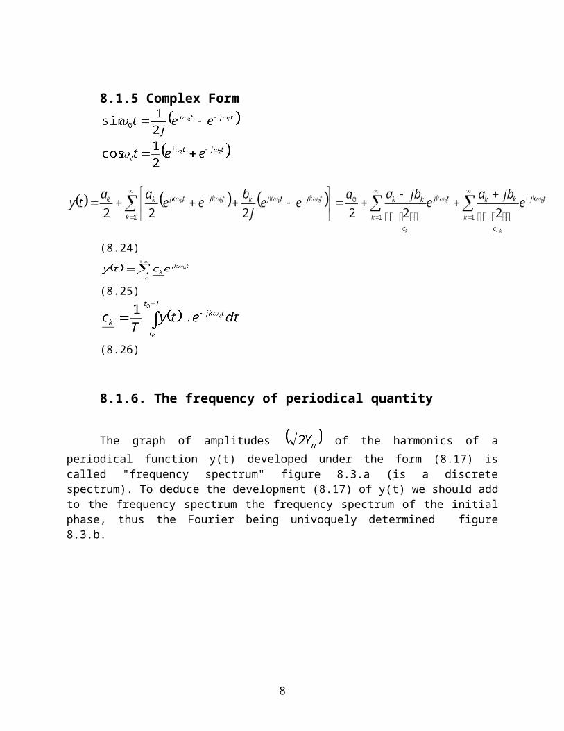
8.1.5 Complex Form

(8.24)

(8.25)

6

(8.26)

8.1.6. The frequency of periodical quantity

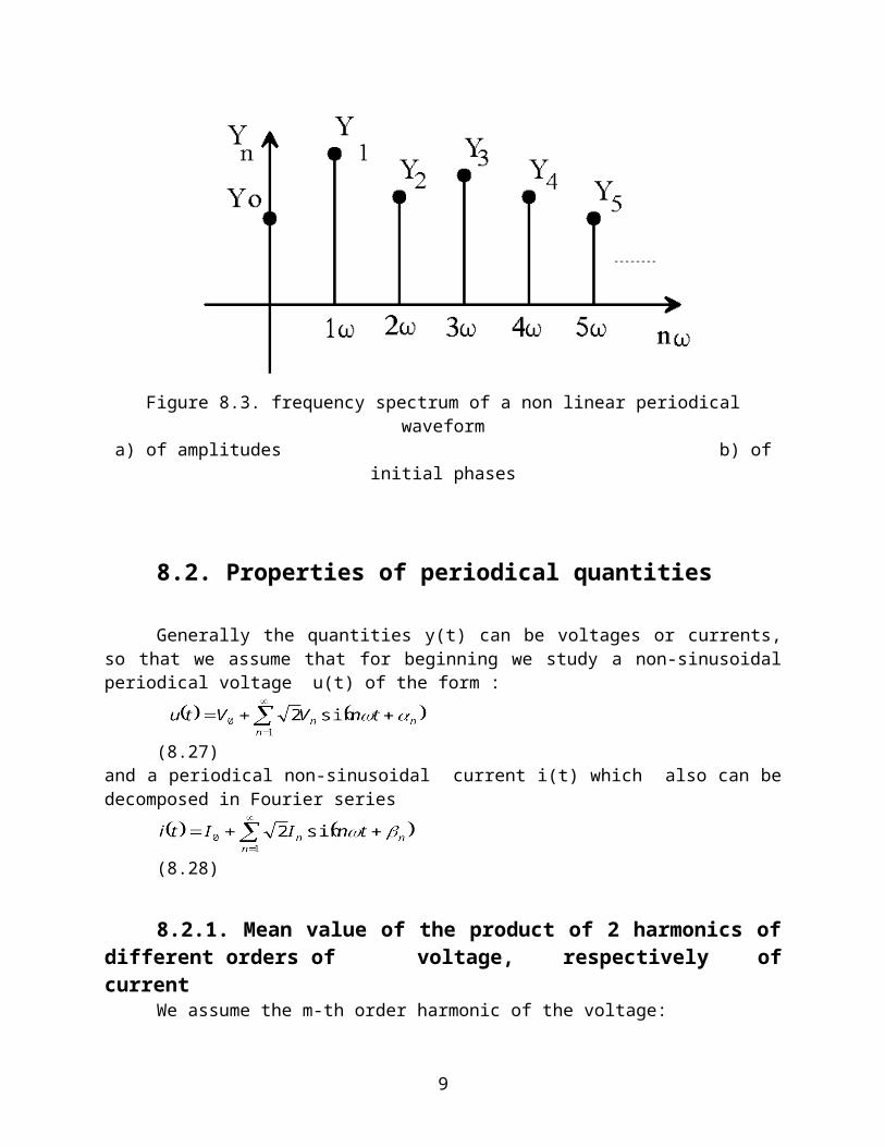
The graph of amplitudes of the harmonics of a periodical function y(t) developed under the form (8.17) is called "frequency spectrum" figure 8.3.a (is a discrete spectrum). To deduce the development (8.17) of y(t) we should add to the frequency spectrum the frequency spectrum of the initial phase, thus the Fourier being univoquely determined figure 8.3.b.

Figure 8.3. frequency spectrum of a non linear periodical waveform a) of amplitudes b) of initial phases

8.2. Properties of periodical quantities

Generally the quantities y(t) can be voltages or currents, so that we assume that for beginning we study a non-sinusoidal periodical voltage u(t) of the form :

(8.27)

and a periodical non-sinusoidal current i(t) which also can be decomposed in Fourier series

(8.28)

8.2.1. Mean value of the product of 2 harmonics of different orders of voltage, respectively of current

7

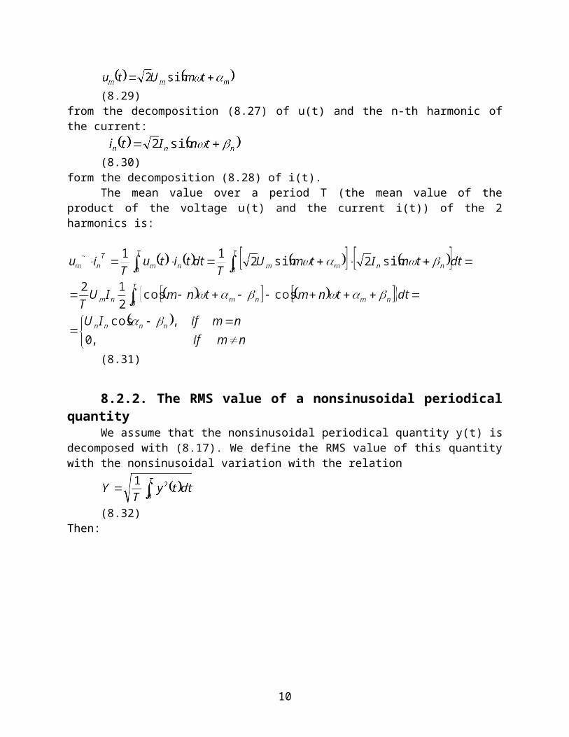
We assume the m-th order harmonic of the voltage: (8.29)

from the decomposition (8.27) of u(t) and the n-th harmonic of the current: (8.30)

form the decomposition (8.28) of i(t).The mean value over a period T (the mean value of the product of the voltage u(t) and the

current i(t)) of the 2 harmonics is:

(8.31)

8.2.2. The RMS value of a nonsinusoidal periodical quantityWe assume that the nonsinusoidal periodical quantity y(t) is decomposed with (8.17). We

define the RMS value of this quantity with the nonsinusoidal variation with the relation

(8.32)

Then:

(8.33)

But

(8.34)

Substituting (8.34) in (8.33) and then in (8.32) we find:

(8.35)

where Yd is called the distorting residue of the quantity y(t) and it is equal to the RMS value of the high harmonics:

(8.36)

Then the RMS value of the voltage u(t) given by (8.27) is:

8

(8.37)with the distorting residue of voltage:

(8.38)

The RMS value of the current i(t) decomposed with (8.28) is:(8.39)

with the distorting residue of current:

(8.40)

8.2.3 Factors Characterising the Nonsinusoidal Periodic WaveformWe consider a nonsinusoidal periodic waveform developed under the form (8.17).

8.2.3.1 The Peak (Amplitude) Factor kvThe peak factor (or amplitude factor) is defined as a ratio between the maximum value of

the periodical quantity (Ymax) and the RMS value Y:

(8.41)

At the sinusoidal periodical quantities:(8.42)

We say that a periodical waveform is flat if and that is keen if .

8.2.3.2 The Factor of Form kf The factor of form kf of a periodical function y(t) is defined as a ratio between the RMS

value and the mean value Y of the periodical function along a half of period:

(8.43)

Here t0 is the moment of zero-crossing of y(t) towards ascendant values.At a sinusoidal periodic waveform:

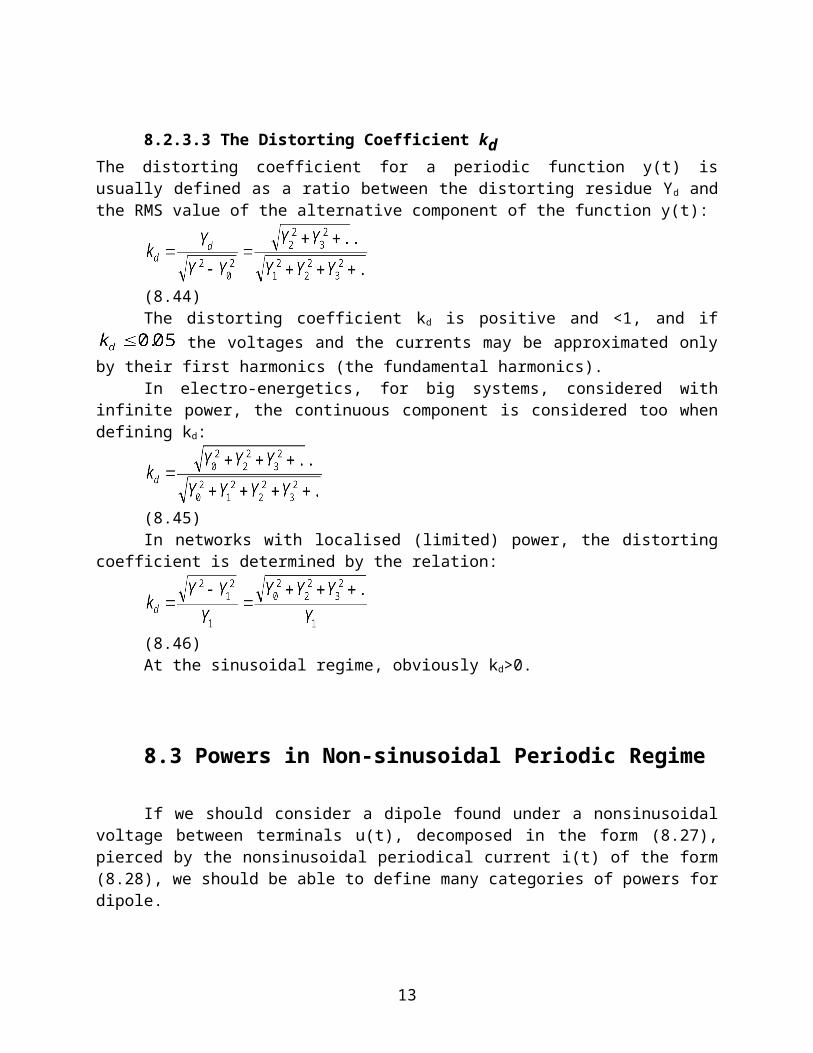
8.2.3.3 The Distorting Coefficient kdThe distorting coefficient for a periodic function y(t) is usually defined as a ratio between the distorting residue Yd and the RMS value of the alternative component of the function y(t):

9

(8.44)

The distorting coefficient kd is positive and <1, and if the voltages and the currents may be approximated only by their first harmonics (the fundamental harmonics).

In electro-energetics, for big systems, considered with infinite power, the continuous component is considered too when defining kd:

(8.45)

In networks with localised (limited) power, the distorting coefficient is determined by the relation:

(8.46)

At the sinusoidal regime, obviously kd>0.

8.3 Powers in Non-sinusoidal Periodic Regime

If we should consider a dipole found under a nonsinusoidal voltage between terminals u(t), decomposed in the form (8.27), pierced by the nonsinusoidal periodical current i(t) of the form (8.28), we should be able to define many categories of powers for dipole.

8.3.1 Instantaneous powerThe instantaneous power is defined using the product of the instantaneous values of

voltage and current:

(8.47)

8.3.2 Active powerThe active power, P defined as the medium value over the common period T (of voltage

and current) of the instantaneous power:

(8.48)

(8.49)

where is the phase difference between the homologous harmonics voltage and current. Then in nonsinusoidal periodical regime, the active power is equal to the sum of the active power of the component of d.c. (U0 . I0 ) and the sum of the harmonics active power.

The active power is measured in watts:

10

8.3.3 Reactive powerThe reactive power is defined as the sum of the harmonics reactive powers:

(8.50)

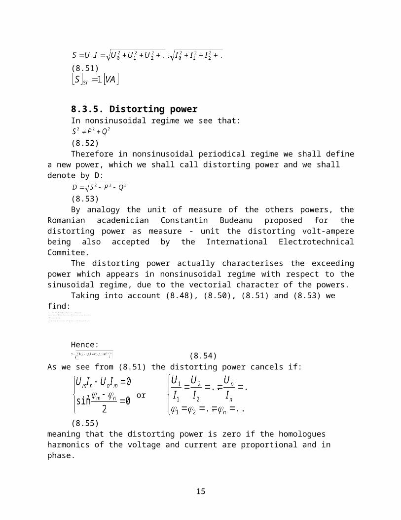
8.3.4 Apparent PowerThe apparent power S is defined as the product of the RMS values of voltage and current:

(8.51)

8.3.5. Distorting powerIn nonsinusoidal regime we see that:

(8.52)Therefore in nonsinusoidal periodical regime we shall define a new power, which we

shall call distorting power and we shall denote by D:(8.53)

By analogy the unit of measure of the others powers, the Romanian academician Constantin Budeanu proposed for the distorting power as measure - unit the distorting volt-ampere being also accepted by the International Electrotechnical Commitee.

The distorting power actually characterises the exceeding power which appears in nonsinusoidal regime with respect to the sinusoidal regime, due to the vectorial character of the powers.

Taking into account (8.48), (8.50), (8.51) and (8.53) we find:

Hence:(8.54)

As we see from (8.51) the distorting power cancels if:

or (8.55)

meaning that the distorting power is zero if the homologues harmonics of the voltage and current are proportional and in phase.

8.3.6 Complementary powerHaving in view that in nonsinusoidal regime the relations (8.53) is valid, actually means

that the deviation from the sinusoidal currents and in phase with the supplying voltage is due to both reactive power and to distorting power. Therefore we define vectorial a global power corresponding to them, which we should call complementary power:

11

(8.56)

8.4. The Power Factor in Distorting Regime

To define the power factor at a dipole in PPNR we proposed few definitions, each of

them trying to reveal some characteristics of this regime:

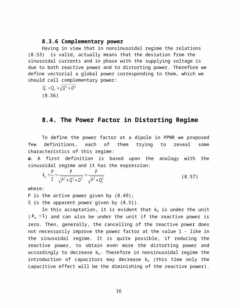
a. A first definition is based upon the analogy with the sinusoidal regime and it has the

expression:

(8.57)

where:

P is the active power given by (8.49);

S is the apparent power given by (8.51).

In this acceptation, it is evident that kp is under the unit ( ) and can also be under the

unit if the reactive power is zero. Then, generally, the cancelling of the reactive power does not

necessarily improve the power factor at the value 1 - like in the sinusoidal regime. It is quite

possible, if reducing the reactive power, to obtain even more the distorting power and

accordingly to decrease kp. Therefore in nonsinusoidal regime the introduction of capacitors may

decrease kp (this time only the capacitive effect will be the diminishing of the reactive power).

To improve the power factor it is necessary to reduce the complementary power Qc

(which changes into reactive power in sinusoidal regime).

b. A second definition is based upon the possibility of identifying the receivers producing

distorting regime with respect to those which do not produce such a regime. In this situation we

must report the apparent power to the fundamental harmonic:

(8.58)

(which should correspond to the maximum active power absorbed by a pure resistive linear

receiver, supplied by a sinusoidal voltage).

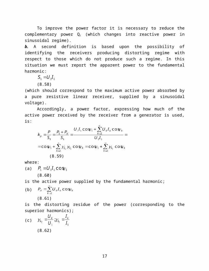
Accordingly, a power factor, expressing how much of the active power received by the

receiver from a generator is used, is:

(8.59)

where:

12

(a) (8.60)

is the active power supplied by the fundamental harmonic;

(b) (8.61)

is the distorting residue of the power (corresponding to the superior harmonics);

(c) (8.62)

represent the weights of the kth harmonics of the voltage, respectively of the current, with

respect to the fundamental harmonic of the voltage, respectively of the current.

Then the power factor in this hypothesis can also be written:

(8.63)

where:(c') (8.64)

is the fundamental power factor;

(c'') (8.65)

is the distorting power factor.

In this case too, the optimal value is also 1 for kp, as in sinusoidal regime, but this thing

must be done in two generally independent ways:

- the cancelling of the active power distorting residue (Pd=0);

- the full compensation of the reactive power on the fundamental harmonic ();

This second definition makes the power factor defined by (8.59) to be not only a

characteristic of the distorting receiver, but to be considered as a factor expressing the interaction

between receiver and network under given operating conditions. It means that if the supplying

network is changed, the power factor changes too, even though the fundamental frequency and

the fundamental nominal voltage remain unchanged.

Under this new acceptation let us also specify that the power factor may also be greater

than 1, this depending on the circulation sense of the distorting residue of the active power:

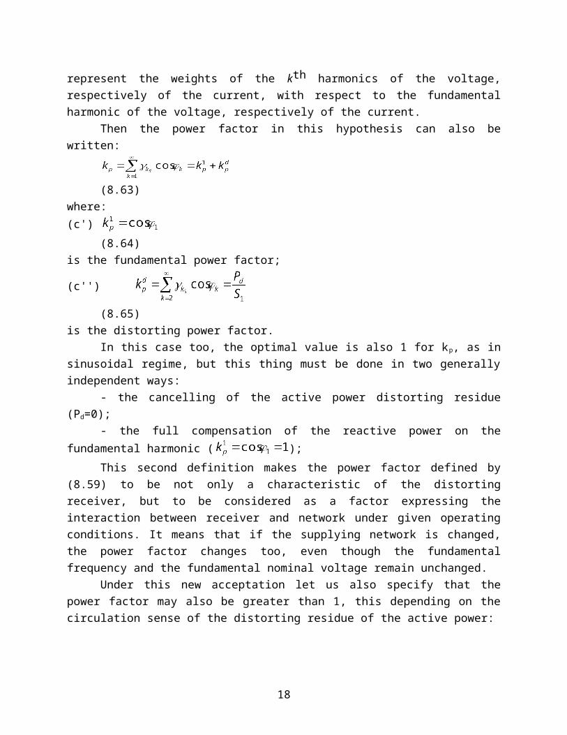
(a) For distorting receivers (generally non-linear) the distorting residue of the active power is

from the receiver towards the network to which it is connected (fig.8.6.)

13

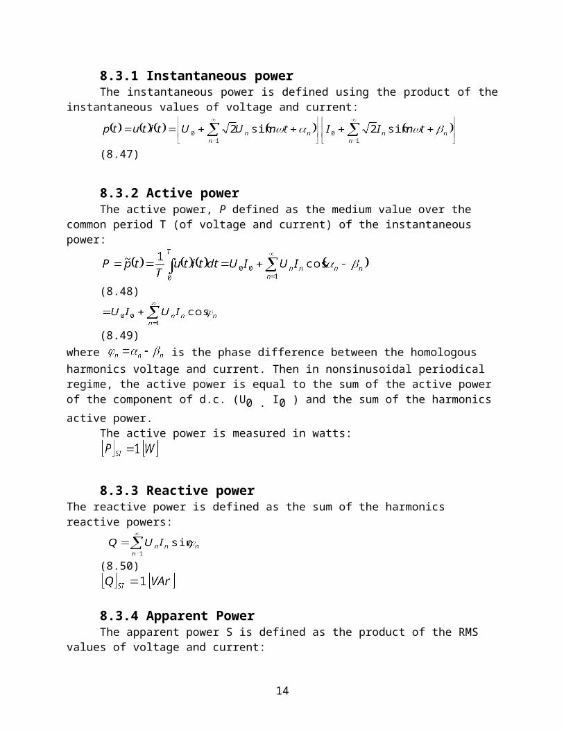
Figure 8.6

In this case:

(8.66)

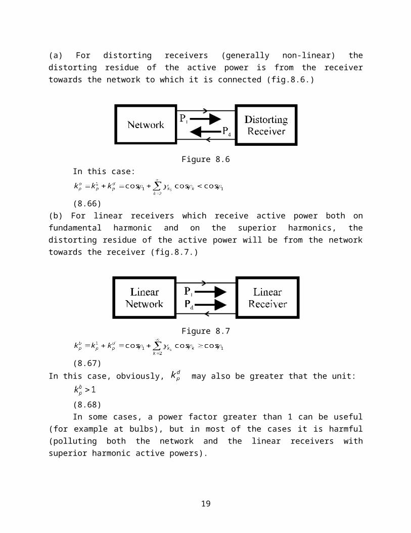
(b) For linear receivers which receive active power both on fundamental harmonic and on the

superior harmonics, the distorting residue of the active power will be from the network towards

the receiver (fig.8.7.)

Figure 8.7

(8.67)

In this case, obviously, may also be greater that the unit:

(8.68)

In some cases, a power factor greater than 1 can be useful (for example at bulbs), but in

most of the cases it is harmful (polluting both the network and the linear receivers with superior

harmonic active powers).

8.5. Linear Circuits in Permanently Periodical Non-sinusoidal Regime

8.5.1. Kirchhoff's Theorems at Linear Circuits Found in PPNR

Considering that Kirchhoff's theorems in instantaneous values were deduced for a quasi-

stationary operating regime of an electric circuit, it means that they keep their validity in PPNR

too. Let us also specify that a function which meets Dirichlet's conditions and allows a Fourier

14

series development is identically zero if both its continuous component and its harmonics are

zero.

8.5.1.1. Kirchhoff's First Theorem

Evidently, we assume a linear network and that the only sources of non-sinusoidal

periodical regime are exactly the network sources. In this case, in order to write the equation

without difficulties, the used index will symbolize the side order and the exponent will

symbolize the harmonic order.

Thus, for every circuit node, at an isolated network having a periodical variation of the

electrical quantities, Kirchhoff's first theorem is written in the general case (in instantaneous

values):

(8.69)

ik(t) from (8.69) represents the current through the side k and it is developed in Fourier

series under the form:

(8.70)

Substituting (8.70) in (8.69), we find:

(8.71)

whence, using the previous observation:

(8.72)

or

(8.73)

As one may notice from (8.72) or (8.73), Kirchhoff's first theorem is separately valid for

each harmonic and can be enunciated as follows:

"The algebraic sum of the currents of the harmonic for a circuit node is always zero, if

the network is linear and the electrical quantities present periodical variations".

15

8.5.1.2. Kirchhoff's Second Theorem

In this case the Kirchhoff's Second theorem remains valid too for a circuit loop:

(8.74)

If the voltage at the kth side terminals presents a periodic variation, having the

development in Fourier series:

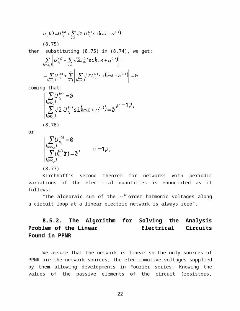
(8.75)

then, substituting (8.75) in (8.74), we get:

coming that:

(8.76)

or

(8.77)

Kirchhoff's second theorem for networks with periodic variations of the electrical

quantities is enunciated as it follows:

"The algebraic sum of the order harmonic voltages along a circuit loop at a linear

electric network is always zero".

8.5.2. The Algorithm for Solving the Analysis Problem of the Linear Electrical Circuits Found in PPNR

We assume that the network is linear so the only sources of PPNR are the network

sources, the electromotive voltages supplied by them allowing developments in Fourier series.

Knowing the values of the passive elements of the circuit (resistors, inductances and capacitors)

and the values of sources which generally are non-sinusoidal periodic, due to the linear character

16

of the network or of the circuit, to solve the analysis problem we can apply the superposition

theorem as follows:

(a) We make the harmonic components of the sources of electromotive voltages and of

current to act one by one; they will determine harmonic currents of order through the sides of

the network;

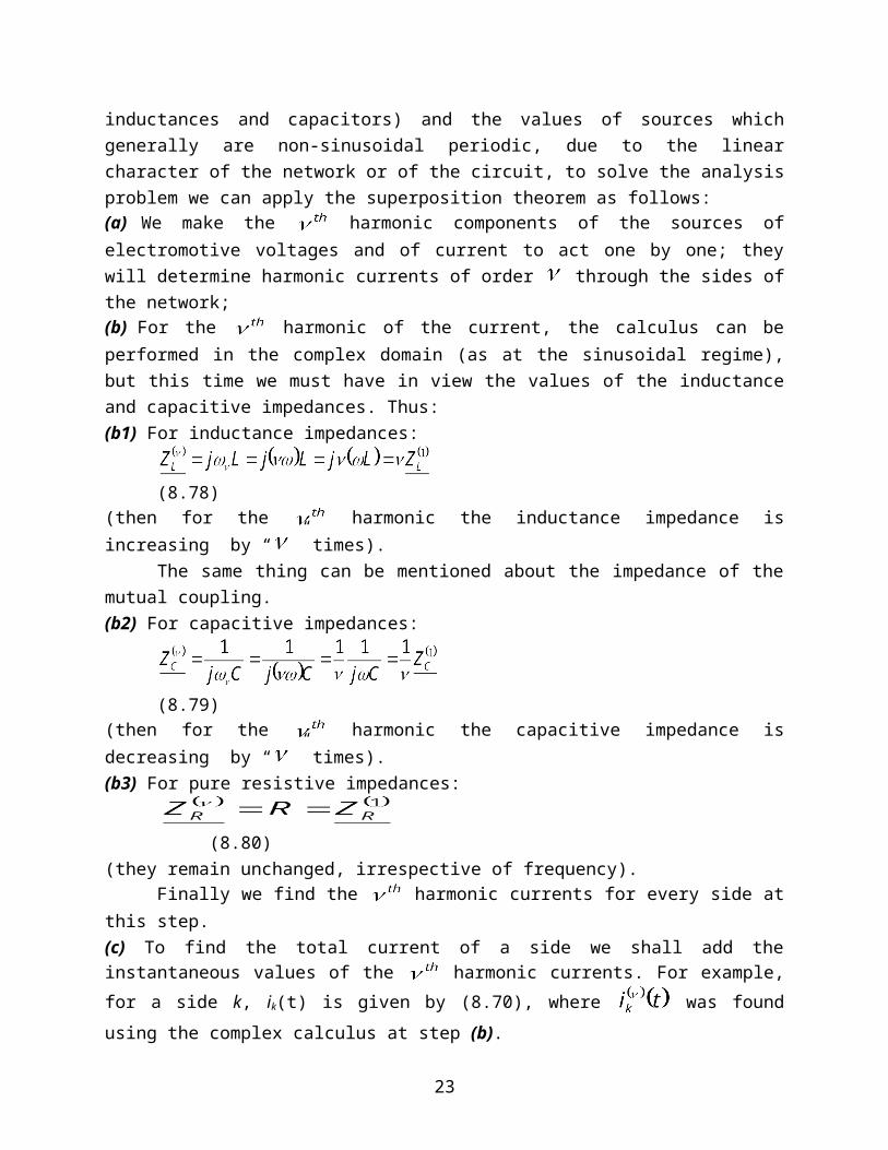
(b) For the harmonic of the current, the calculus can be performed in the complex domain (as

at the sinusoidal regime), but this time we must have in view the values of the inductance and

capacitive impedances. Thus:

(b1) For inductance impedances:(8.78)

(then for the harmonic the inductance impedance is increasing by “ ” times).

The same thing can be mentioned about the impedance of the mutual coupling.

(b2) For capacitive impedances:

(8.79)

(then for the harmonic the capacitive impedance is decreasing by “ ” times).

(b3) For pure resistive impedances:

(8.80)

(they remain unchanged, irrespective of frequency).

Finally we find the harmonic currents for every side at this step.

(c) To find the total current of a side we shall add the instantaneous values of the harmonic

currents. For example, for a side k, ik(t) is given by (8.70), where was found using the

complex calculus at step (b).

8.6 The Behavior of the Idle linear Elements in PPNR (Distorting) regime

We analyze in this paragraph the mode of variation of the current through the ideal linear

elements of the circuit (resistor, coil and capacitor) at their supplying with periodical permanent

non-sinusoidal voltage, using a decomposition in Fourier series of the form:

(8.83)

Each of these elements will absorb a distorting periodically current, with a variation of the form:

17

(8.84)

each harmonic of order k of the current depending only on the kth harmonic of the voltage.

8.6.1. The Behavior of an Idle Resistor at the Supplying with a Non-sinusoidal Periodic Voltage

Figure 8.9

The supplying voltage of a linear resistor is periodic non-sinusoidal, having the

development in Fourier series of the form (8.83). In this case the relation between voltage and

current is:

(8.85)

then:

(8.86)

The current will result under the form (8.84) from (8.86):

(8.87)

where:

18

(8.88a)

(8.88b)

(8.88c)

Then:

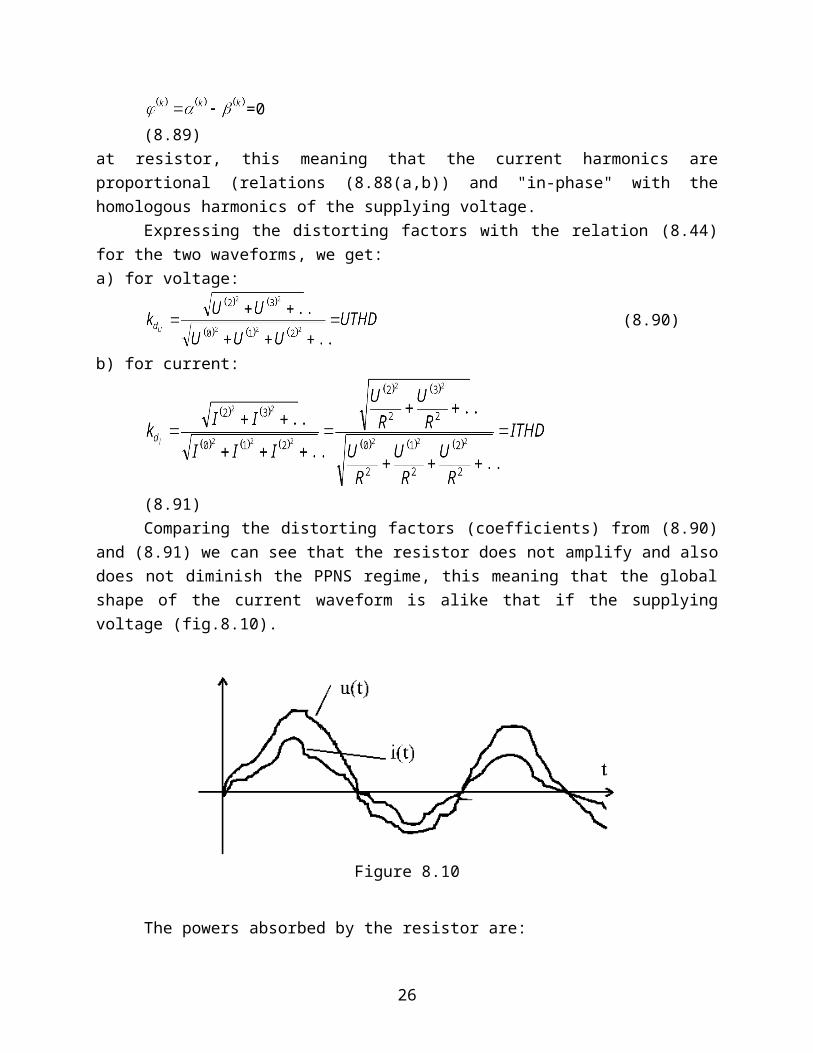
=0 (8.89)

at resistor, this meaning that the current harmonics are proportional (relations (8.88(a,b)) and "in-

phase" with the homologous harmonics of the supplying voltage.

Expressing the distorting factors with the relation (8.44) for the two waveforms, we get:

a) for voltage:

(8.90)

b) for current:

(8.91)

Comparing the distorting factors (coefficients) from (8.90) and (8.91) we can see that the

resistor does not amplify and also does not diminish the PPNS regime, this meaning that the

global shape of the current waveform is alike that if the supplying voltage (fig.8.10).

Figure 8.10

The powers absorbed by the resistor are:

1. the active power:

19

(8.52)

where:

a) U is the RMS value of the supplying voltage:

b) I is the RMS value of the absorbed current:

2. the reactive power:

(8.95)

3. the apparent power:

(8.96)

4. the distorting power:

Because

(8.97)

then the conditions (8.55) are meet, the distorting power is zero. This thing can be also

performed if we should have calculated it starting from its definition:

(8.98)

(from (8.92), (8.95) and (8.96)).

Also from the expression of the distorting power we can see that its null value results in

no influence of the resistor over the non-sinusoidal permanent periodic current with respect to

the variation mode of the supplying voltage.

The power factor in this case is:

1-using the definition (8.57):

(8.99)


(8.100)

where:

(8.101a)

20

(8.101b)

From (8.100), because in practice:(8.102a)

(8.102b)

(that is the high harmonics generally have an amplitude which is smaller than the fundamental

one, at both voltage and current), it means that the power factor may also be greater than 1.

Then, practically the linear resistor absorbs active power both on the fundamental

harmonic at a unitary power factor ( ), and on the superior harmonics. This effect can

be useful when such a resistor is used for heating purposes, but harmful in the other practical

situations.

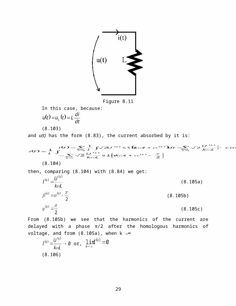
8.6.2. Behavior of an Idle Coil at the Supplying with Non-sinusoidal Periodic Voltage

Figure 8.11

In this case, because:

(8.103)

and u(t) has the form (8.83), the current absorbed by it is:

(8.104)

then, comparing (8.104) with (8.84) we get:

21

(8.105a)

(8.105b)

(8.105c)

From (8.105b) we see that the harmonics of the current are delayed with a phase π/2 after the

homologous harmonics of voltage, and from (8.105a), when k →∞

or, (8.106)

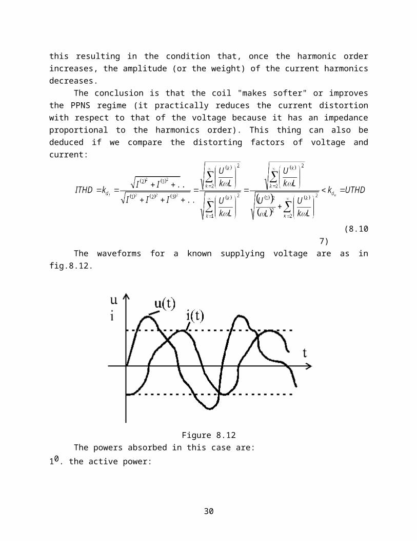
this resulting in the condition that, once the harmonic order increases, the amplitude (or the

weight) of the current harmonics decreases.

The conclusion is that the coil "makes softer" or improves the PPNS regime (it practically

reduces the current distortion with respect to that of the voltage because it has an impedance

proportional to the harmonics order). This thing can also be deduced if we compare the distorting

factors of voltage and current:

(8.107)

The waveforms for a known supplying voltage are as in fig.8.12.

Figure 8.12

The powers absorbed in this case are:

22


(8.108)

Observation: If the supplying voltage has also a continuous component, obviously

(8.109), but the variation of u(t) will no longer be around the horizontal axis, but around the

horizontal line (8.110). Analogous for the current.


(8.111)


(8.112)

40. the distorting power (also non-zero this time):

(8.113)

Then the distorting power shows us that in this case the distortion degree of the voltage and

current is different.

The power factor is:


(8.114)


(8.115)

From both definitions of the power factor one can notice that the linear coil supplied by

an PPNS voltage does not absorb active power neither on the fundamental harmonic nor on

superior harmonics. In exchange from (8.111) and (8.113) we can see that it absorbs both

reactive power (Q>0) and distorting power (D>0), meaning that besides the reactivity that an idle

coil has in the case of a sinusoidal regime, in non-sinusoidal regime the idle coil also influences

the degree of distortion of the current with respect to the supplying voltage - thing also found at

the expression of the distorting factor of voltage and current.

8.6.3. Behavior of Idle Capacitor at Supplying with Non-sinusoidal Periodic Voltage

23

Figure 8.13

When supplying a capacitor with a periodic non-sinusoidal voltage u(t), given by (8.83),

the current variation through the capacitor is obtained from the relationship between voltage and

current:

(8.116)

hence:

(8.117)

Comparing (8.117) with (8.84) we find:(8.118a)

(8.118b)

(8.118c)

When k→∞, we find that:

, (8.119)

then the linear capacitor supplied with a non-sinusoidal periodic voltage distorts even more the

current waveform (simultaneously with the increasing of the harmonic order, the RMS of the

current corresponding to the respective harmonic increases, too). This thing can also be seen if

we compare the distorting factors of the two waveforms:

(8.120)

The waveform of the periodic current i(t) at the supplying with a PPNS voltage u(t) is

given in fig.8.14.

24

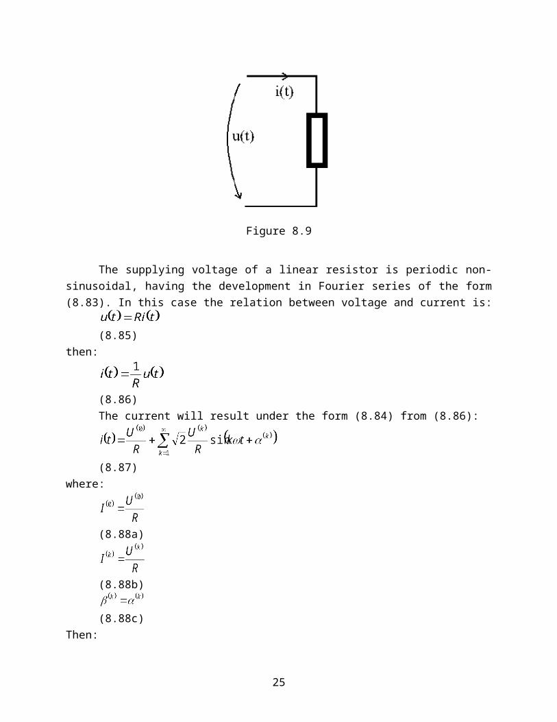
Figure 8.14

The powers absorbed in this case are:


(8.121)


(8.122)

Q<0 means that, actually, the capacitor gives reactive power, both on the fundamental harmonic

and on superior harmonics.


(8.123)

40. the distorting power:

(8.124)

The distorting power presence in this case too shows us a different distorting degree at

voltage and respectively at current.

The power factor is in this case:

1-with the definition (8.57):

25

(8.125)


(8.126)

Like in the case of the idle coil, using both modalities for the definition of the power

factor, we see that also the idle capacitor supplied by a non-sinusoidal periodic voltage does not

absorb active power neither on the fundamental harmonic nor on the superior harmonics. In

exchange from (8.122) we see that an idle capacitor delivers in network reactive power both on

the fundamental harmonic and on superior harmonics (Q<0), as a consequence of receiving

apparent power. Except that a part of this power turns into distorting power, distorting even more

the current with respect to the supplying voltage as we saw from (8.120) (with respect to the

distorting factor for the current relative to that of the voltage).

8.6.4 Behavior of Simple Circuits at Supplying with PPN Voltage

8.6.4.1. Behavior of a RLC Series Circuit Supplied by a Non-sinusoidal Permanent Periodic

Voltage (NPPV)

8.6.4.1.1. Analysis of a RLC Series Circuit Supplied by a NPPV

Figure 8.15

We consider the RLC series circuit supplied by a NPPV of the form (8.83). To find i(t)

we use the superposition theorem in this case, considering the circuit equation:(8.152)

or:

26

(8.153)

Under the action of the supplying voltage of the kth harmonic, the circuit equation is:

(8.154)

or in complex:

(8.155)

where:(8.156)

From (8.155) and (8.156) we find I(k):

(8.157)

Here:

(8.158)

is the impedance of the RLC series circuit corresponding to the kth harmonic. Obviously:

(8.159)

With (8.159) and (8.156) in (8.157) we find:

(8.160)

Then the instantaneous value of the kth harmonic current is:

(8.161)

The total current through circuit, based upon the superposition theorem, is:

(8.162)

10. The active power:

27

(8.163)

20. The reactive power:

(8.164a)

where:

(8.164b)

(8.164c)

30. The apparent power:

(8.165)

40. The distorting power:

(8.166)

The power factor is:


(8.167)

2-using definition (8.):

28

(8.168)

Concluding about the RLC series circuit supplied by a NPPV, we can say that:

(a) - is always absorbing active power both on fundamental harmonic and on the superior

harmonics (relation (8.163));(b) - the reactive power may be absorbed on certain harmonics, ki, for which:

(8.169)

but may be released on other harmonics, kl, for which:

(8.170)

Generally speaking the total reactive power Q may be absorbed (when Q>0 or QL>|QC|)

or released (when Q<0 or QL<|QC|).

(c) - the appearance of a nonzero distorting power clearly emphasizes a distorting degree of the

current absorbed by this circuit different from its supplying voltage;

(d) - the power factor, irrespective of the definition used for its definition, is always signalising

an active power absorbed by the RLC series circuit both on fundamental harmonic and on

superior harmonics.

8.6.4.1.2. Resonance of the RLC Series Circuit Supplied by a NPPV. Filter of Harmonics

As we saw from (8.158), the complex impedance corresponding to the kth harmonic is:

(8.171)

where:(8.172)

is the inductance reactance corresponding to the kth harmonic, and:

(8.173)

is the capacitive reactance corresponding to the kth harmonic.

As we can see from (8.172) and (8.173), the two reactances are differently modifying

with respect to frequency: the inductive reactance grows directly proportional with the frequency

whereas the capacitive reactance decreases in inverse proportion with the frequency.

On the whole the total reactance X(k) of the RLC series circuit increases when the

frequency increases. In this situation, if on the fundamental harmonic:

29

(8.174)

it is possible to exist a certain frequency k0 for which X(k) should cancel:

(8.175)

where:

(8.176)

Obviously, the reactance cancels on the k0 harmonic only if is a natural number.

For values of k>k0, the reactance X(k) becomes positive, growing together with k. If there

is a k0 satisfying (8.175), then for the th harmonic the positive reactance has the same absolute

value as the negative reactance of the fundamental harmonic:

(8.177)

Concluding, we can say that for a RLC series circuit supplied by a NPPV, even though no

resonance phenomenon should occur on the fundamental harmonic, it may be possible for it to occurs on a superior harmonic, k0, if the condition (8.177) is met. The appearance of the

voltages' resonance phenomenon on a superior harmonic in the RLC series circuit may result in

the designing of some passive filters L-C for the absorption of the superior harmonics when

these appear in the electrical networks. In such situations we can say that a compensation of the

distorting regime on a superior harmonic takes place, through the local absorption of the reactive

power corresponding to that harmonic k:

(8.178)

and of the distorting power, which practically represents the connection between the kth

harmonic and the other harmonics (including the fundamental one):

(8.179)

This thing becomes possible because on the kth harmonic the impedance corresponding

to this harmonic, Z(k), has a zero imaginary part:

(8.180)

and in the absence of a resistance:

(8.181)

meaning that through such an impedance the current may be considered as much as possible

(theoretically infinite).

30

Usually the harmonic passive filters (the LC circuits) are assembled in parallel with the

network in which harmonic components of voltage and current occur, in order to face the local

absorption of the reactive and distorting powers given by (8.180) and (8.181). the variation of a

filter impedance with respect to frequency for a LC filter corresponding to the 5th harmonic is

given in fig.8.16.

Figure 8.16

If for the frequency of the proper harmonic (k=5 or f=5x50=250 Hz) the total impedance

of the filter is zero, for frequencies smaller than 250 Hz, Z(k) has a capacitive character (X(k)<0),

and for frequencies greater than 250 Hz, Z(k) has an inductive character (X(k)>0). Such a filter

behaves differently for neighbouring harmonics: it behaves like a filter for harmonics different

from k=5 too, but in a distinct manner (for example it filters the 11th harmonic better than the

13th harmonic, s.o.).

Let us also specify that in practice for high frequencies combined filters are usually used,

due to the lower weight of the higher harmonics at the increasing frequency and because the

impedance for the harmonics to be combined is resulting small enough to produce an efficient

filtering.

31

Documents

curs 6.doc