D A S E

A P S? E

I1

Abhiroop Mukhopadhyay2 and Soham Sahoo3

July 16, 2013

1The authors wish to thank Emla Fitzsimons, Victor Lavy, seminar participants at theInstitute of Economic Growth (Delhi) and the Indian School of Business (Hyderabad); par-ticipants of the Growth and Development Conference (Delhi), the Italian Doctoral Workshopin Economics and Policy Analysis (Turin), IZA at DC Young Scholar Program (WashingtonDC), NEUDC (Dartmouth), and Asian Meeting of the Econometric Society (Delhi) for theircomments. This research was funded by a research grant from the Planning and PolicyResearch Unit, Indian Statistical Institute, Delhi. Abhiroop Mukhopadhyay conducted re-search on this paper when he was Sir Ratan Tata Senior Fellow at the Institute of EconomicGrowth, Delhi (2010-11).

2Economics and Planning Unit, Indian Statistical Institute (Delhi): abhiroop@isid.ac.in

3Economics and Planning Unit, Indian Statistical Institute (Delhi): soham9r@isid.ac.in

Abstract

This paper investigates if better access to secondary education increases enrollment in pri-

mary schools among children in the 6-10 age group. Using a household level longitudinal

survey in a poor state in India, we find support for our hypothesis. The results are robust

to endogenous placement of secondary schools and measurement error issues. Moreover, the

marginal effect is larger for poorer households and boys (who are more likely to enter the

labour force). We also find that households that invest in health have a larger marginal

effect. We also provide some suggestive evidence that this effect may be quite widespread in

India.

Keywords: Primary schooling, school enrollment, school attendance, secondary

schooling, human capital, returns to schooling

JEL codes: I2, I20, I25

1 Introduction

The second Millennium Development Goal (MDG) of the United Nations aims at uni-

versalization of primary education by 2015. Despite best attempts and significant rises

in enrollment in most developing countries, recent findings suggest that the target is

unlikely to be met1. While access to primary schooling has improved substantially, high

dropout rates are still a critical problem2. In India, the major public policy initiatives

like Sarva Shiksha Abhiyan (Education for All), the provision of a midday meal, free

textbooks, uniforms etc. aim to universalize elementary education and reduce dispar-

ity across regions, gender and social groups. In this context, two suggestions have been

popular: to reduce the access barrier through the provision of community-based primary

schools; and to improve the quality of schools in terms of physical infrastructure, teacher

quality etc. This paper raises a third issue: Does the possibility of continuation into

higher levels of schooling affect primary schooling outcomes? In particular, we seek to

investigate the effect of access to secondary education on primary school participation.

The decision of investment in the human capital of children is crucially linked to

the perceived economic returns to education (Manski, 1996; Nguyen, 2008; and Jensen,

2010). The received wisdom from studies conducted in the past two decades is that the

returns to education are concave, i.e., the marginal effect of an increment in the number

1A Fact Sheet published by the United Nations in 2010 reveals that although enroll-ment in primary education in developing regions has increased from 83 percent in 2000to 89 percent in 2008, yet this pace of progress is insufficient to meet the target by 2015.About 69 million school age children were out of school in 2008.

2Statistics published by the United Nations show that the proportion of pupils inIndia starting grade 1 who reach last grade of primary was only 68.5 percent in 2006(http://unstats.un.org/unsd/mdg/SeriesDetail.aspx?srid=591). The report on elemen-tary education in India published by the District Information System for Education(DISE) shows that the average dropout rate in primary level (grade 1 to 5) between2006-07 and 2007-08 was 9.4 percent.

3

of years of primary schooling is larger than the effect at higher levels (Psacharopoulos,

1994 and Psacharopoulos and Patrinos, 2004). However, several recent studies show

that the private returns to each extra year of education, in fact, rise with the level of

education. A very recent paper by Colclough et. al. (2010) refers to several studies on

different countries that find this changing pattern of returns to education. Schultz (2004)

finds that private returns in six African countries are highest at the secondary and post-

secondary levels. Kingdon et. al. (2008) find a convex shape of the education-income

relationship in eleven countries.

Studies specific to India have also shown similar results (Kingdon, 1998; Duraisamy,

2002 and Kingdon and Unni, 2001). On the other hand, some other studies show that

while the actual rate of return to primary schooling is high, parents believe that the first

few years of schooling have lower returns than in the later years (Banerjee and Duflo,

2005 and 2011). These observations suggest that households may perceive education

investment as lumpy; that significant economic returns require continuation to at least

high school - households may find it worthwhile to educate their children only if they

can reach that level. In light of this, better access to a post-primary school represents

reduction in the cost of post-primary schooling and increases the possibility of continua-

tion into higher levels of schooling. In doing so, it can become an important determinant

of primary school participation.

This paper aims to empirically test the hypothesis that access to secondary schools

affects primary schooling outcomes. Although the importance of access to schooling in

determining educational outcomes has been well recognized in the literature (Duflo, 2001

and 2004; Filmer, 2007; Glick and Sahn, 2006; Orazem and King, 2007), most of it is

on access to primary schooling and its effect on children. Therefore a major supply side

4

intervention for policy makers has been to increase the availability of primary schools

to the community to encourage more children to go to school. One commonly used

measure of access is distance to school. Different studies have found that a reduction in

distance to school improves enrollment, reduces dropout and improves test scores (Lavy,

1996; Bommier and Lambart, 2000; Brown and Park, 2002; Handa, 2002; and Burde

and Linden, 2012).

Most of the literature addressing access examines the linkage between schooling out-

comes at a particular level with access to that level of schooling. This is true even

when studies look at access to secondary schooling. For example, Muralidharan and

Prakash (2012) look at the impact of an incentive to provide cycles to girls going to

secondary schools on their enrollment. Similarly, Pitt et. al. (1993) look at the effects

of secondary schools on enrollment of children aged 10-14. Therefore, they have a static

view of concentrating solely on the current cost of schooling. However, difficult access to

post-primary schooling that reflects the future cost of schooling hinders the possibility

of continuation to a higher level of education and can hence adversely affect schooling

decisions even at the primary level. Only a few studies acknowledge the importance of

access to post-primary schooling in determining outcomes at the primary level.

Lavy (1996) uses a cross-sectional data-set for rural Ghana and shows that distance to

post-primary schools negatively affects primary school enrollment. He suggests that the

effective fees for post-primary schooling should be reduced to induce more participation

at the primary level. Results similar to Lavy (1996) have been found in other cross

sectional studies by Burke and Beegle (2004) on Tanzania, by Vuri (2008) on Ghana and

Guatemala and by Lincove (2009) on Nigeria. Hazarika (2001) uses a cross-sectional

data-set on rural Pakistan and finds no impact of access to post-primary school on

5

primary school enrollment of girls. His study indicates that if gains from post-primary

schooling are low, as is the case for girls in Pakistan, access to it has no effect on

primary school outcomes. Almost all these studies base their analysis on cross-sectional

data, hence they are unable to control for time-invariant unobserved heterogeneity at the

household level. Moreover, apart from Lavy (1996), there is no discussion on endogenous

placement of schools, which can be a potential source of bias in the estimates. Lavy

(1996), however, does not discuss placement of secondary schools as they are considered

to be very far away from the sampled households. Andrabi et. al. (2013) also point out

to another mechanism that may link secondary schooling access and primary schooling.

They posit that secondary schools may create private school teachers in the future,

hence affecting primary schooling outcomes in the future. This is inherently a long run

mechanism: their paper looks at data 17 years apart. In this paper the mechanism we

look at is much more short term and hence completely different.

This paper uses a household level longitudinal survey of 43 villages in Uttar Pradesh,

a state in India, to test the hypothesis that better access to secondary education increases

enrollment and attendance among children in the primary school going age group. It

takes advantage of two education policies, during the period of the study, that led to

a decrease in inequality of access to secondary schools in the state of Uttar Pradesh.

First, under the 10th five year plan of India (2002-2007), a scheme of Area-Intensive

Programme for Educationally Backward Minorities was initiated3. In line with this

goal, special emphasis was given to extending access to schools in educationally back-

ward areas with higher concentration of Scheduled Castes (SC) and Scheduled Tribes

(ST) population. Second, in addition to the national policy, the Uttar Pradesh state

3http://planningcommission.nic.in/plans/planrel/fiveyr/10th/volume2/v2_ch4_1.pdf

6

government introduced a scheme in 1997 to promote girls’ secondary education. Under

the scheme, any new private girls only secondary school opened in a hitherto uncovered

block headquarter, was made eligible for a one-time infrastructure grant of Rs. 1 million

(Jha and Subrahmanian, 2005). Once this led to the opening of girls secondary schools,

boys were allowed into these girls schools in order to make them cost-effective. Thus,

this policy led to opening of new secondary schools in places which were lagging behind

in the past. This paper takes advantage of this environment where changes in access

to secondary schools over the period of study are more likely to reflect these policy

initiatives rather than a demand driven endogenous placement.

Using a fixed effects regression, the paper finds that there is indeed a positive effect of

better access to secondary education on primary school participation. The results do not

change even after we account for potential endogenous placement of secondary schools

and measurement error issues. Moreover, we find that the effect is heterogeneous: the

marginal effect is larger for smaller villages and for villages closer to bus stops. The

effect is also larger for poorer households and boys (who are more likely to enter the

labour force). We also find a larger marginal effect for households that invest in health

through immunization. Stratifying the sample by age cohorts, the paper finds larger

effects on the enrollment of younger children and on the attendance of older children.

Using a nationally representative survey for India (National Sample Survey 2007-08),

we also provide some suggestive evidence that this effect may be quite widespread.

This study contributes to the existing literature by extensively examining how devel-

opments at higher levels of education influence decisions at much lower levels. We point

out to the lumpiness of human capital investment: that education may be attractive

when children can have a less costly way of acquiring education all the way to secondary

7

school. This backward linkage from secondary school access to primary schooling out-

comes is very different from the question that most of the literature addresses: the

static view of whether primary (secondary) school access affects primary (secondary)

schooling. Among papers that do address a question similar to one asked in this paper,

our paper provides a tighter research design employing household (hence, village) fixed

effects techniques. Moreover,we attempt to validate our result using instruments that

are plausible and by providing a battery of robustness checks that are consistent with

our hypothesis that it is the continuation possibility that seems to drive our results and

not other confounding factors. Our robustness checks, in particular, attempt to rule of

other mechanisms and give support to our hypothesis, something that the other papers

addressing this question do not attempt.4

The paper is organized as follows: Section 2 describes the data used for our analysis.

Section 3 explains the empirical methodology. Section 4 reports the results obtained

from the main regressions. In section 5, we show that our results are robust. Section 6

investigates if there are other pathways that explain our results. In section 7, results are

provided that show that the impact of secondary school access is heterogeneous. Section

8 uses the NSS data to check whether our hypothesis can be extended at the all India

level. The final section discusses the conclusions of the paper.

4Our study relates very well to the recent policy environment in India, where the Min-istry of Human Resource Development has developed a framework for universalizationof access to and improvement of quality at the secondary stage. Following Sarva Shik-sha Abhiyan, a national mission on Rashtriya Madhyamik Shiksha Abhiyan (RMSA), oruniversalization of secondary education, has been set up.

8

2 Data

To test our hypothesis, we provide evidence using data from a longitudinal follow up of

households first surveyed as a part of the World Bank’s Living Standards Measurement

Study (LSMS) in Uttar Pradesh, a state in India (this survey is also called the Survey

of Living Conditions, or SLC). This is a two-period panel data on rural households in

43 villages selected from nine districts in eastern and southern Uttar Pradesh5. The

baseline data was collected in 1997-98 under LSMS. The second round of data was col-

lected in 2007-08 by the authors; the data collection was funded by the University of

Oxford and the World Bank 6. The survey comprised a village questionnaire that con-

tained information on, among other things, access to the nearest primary and secondary

school and a household questionnaire that had detailed information on various aspects

of standard of living, including the schooling status of each child in the household.

For the purpose of our study, we use information on households with children in the

6-10 age group. There were 402 such households in 1997-98 and 346 in 2007-087. Among

these households, there were 210 households with children in the relevant age group in

both 1997-98 and 2007-088. We use data on these households in our panel methods9.

5Uttar Pradesh is usually considered one of the most backward regions in the country.Our sample includes 9 districts.The number of villages in each district vary from 3 to 6per district.

6Both surveys were conducted during the same time of the year - December to April.The data collected in 1997 was verified to the extent possible during the second survey.Household attrition rate for the sample was 12.16 percent.

7There are 705 children in the relevant age group in 1997-98 and 566 children in2007-08.

8Appendix Table A1 summarizes the changes over time for these households. Wediscuss some of the key changes in the discussion that follows.

9Our most restrictive analysis using the balanced panel of households uses informationon 722 children over the two years.

9

These 210 included households do not vary significantly from the excluded ones in

terms of baseline (2007-08) characteristics (Appendix Table A2). The only characteristic

that is significantly different between them is household size. The included households

have, on an average, 0.69 members more.

Our two variables of interest are the proportion of children aged 6-10 in households

who are enrolled in schools, defined as enrol, and the proportion of children in the

same age group in households that attend school. The SLC has detailed information on

attendance. It reports the number of days in the past 7 days that the child attended

school10. We define attend as the proportion of children in the household who have

attended school at least three days in the last week.

According to the estimates from the panel of households, while enrol was 67 percent

in 1997-98, it had increased to 83 percent by 2007-08. Based on our definition, while the

attendance share was 63 percent in 1997-98, it had risen to 82 percent by 2007-0811.

We use information on distance-to-schools that have been collected during the village

survey. Distance to the nearest primary, middle and secondary schools is measured

from the village centre and reported in kilometers. The average distance to the nearest

primary school has reduced from 0.76 km to 0.1 km and to the nearest middle school

from 2.46 km to 1.46 km12. However, because both primary and middle schools were

already very close on average to the villages in 1997-98, the change in them is modest.

10Consistent with the baseline survey, holidays and unusual attendances because offamily events are factored in while asking this question. For this small sub-sample,attendance on the last normal week is asked. While such self reported data are notperfect, we are constrained not to change questions for the sake of uniformity.11The corresponding enrollment rate for children in the 6-10 age group increased from

65 percent in 1997-98 to 83 percent in 2007-08. The rise in enrollment rate has beenhigher for girls (from 59 percent to 84 percent) as compared to boys (from 73 percentto 82 percent). Attendance rates show a similar trend.12Middle schools are also called Upper Primary in the education literature.

10

The change in the distance to the nearest secondary school has been spectacular, though,

the average distance has reduced from 5.59 km to 3.44 km (Figure 1).

To investigate if the change in distance to nearest secondary schools over time de-

pends on baseline household characteristics, in Appendix Table A3, we report a regres-

sion of a variable that measures change in distance of nearest secondary school (1997-98

minus 2007-08) on baseline characteristics. A greater value of this variable implies a

greater change. We find that the change in distance is negatively correlated to the

proportion of literate mothers in a household. Since mother’s literacy is often a strong

indicator of children’s education, this implies that, over time, households with less lit-

erate mothers now have greater access to secondary schools. We account for this in

our empirical model. Also, change in distance has been less for the Muslim households.

No other observed variable considered (father’s literacy, household head literacy, gen-

der of household head, land ownership, caste, and household size) is significant. Thus

the change in distance to secondary schools does not seem to be correlated to baseline

covariates of demand. If anything, households with typically lower baseline demand for

education have seen larger changes in access1314.

Given the almost insignificant relationship between changing access to secondary

schools and covariates of demand, what explains then, the temporal change in access?

As mentioned before, the state government policy promoted opening up of new secondary

schools in blocks (administrative units which include many villages) where there was no

single sex secondary school for girls. These were subsequently opened to boys by most

13This equalization is equally true when we use estimates of baseline demand at thevillage, block or district level.14The survey conducted in 1997-98 does not ask about whether the nearest secondary

school is private or public. Hence we are not able separate the effects by type of school.

11

schools to make them cost effective. Moreover, the 10th five year plan aimed at providing

better access to communities with higher concentration of SC and ST population. To

investigate if these indeed were correlated with the changing access to secondary schools,

we include two variables: whether the block had any single sex girls secondary school

at the baseline (Girls_School), and the proportion of SC/ST households in the village

(SCST_Prop). Results show that both the variables are significant in the regression.

The distance to nearest secondary school has reduced more in places where there was

no girls secondary school before15. The change is also higher in places with more SC/ST

concentration. These results suggest that placement of new secondary schools was not

driven by demand for education. Rather, the government policies were instrumental in

providing better access to areas which were educationally backward.

Pooling the data from both rounds, we find a significant and negative correlation of

-0.20 between the proportion of enrolled children at the primary level and distance to

the nearest secondary school. However, this correlation coefficient does not take into

account any other confounding factors that may have changed over time. Therefore, in

the next section, we specify econometric models and carry out multivariate analysis to

look into the hypothesized causation more carefully.

15Data for Girls Secondary Schools at the block level are sourced from The 7th AllIndia Education Survey (NCERT) conducted in 2002. Ideally, we would have liked toconduct the exercise with data prior to 1997. However, data from an earlier period werenot available to the authors. But it is easy to see that this doesn’t bias our resultstoo much. If schools had already opened up in response to the policy by 2002, wewould expect that the relation between change of access to secondary schools and thisvariable would be be insignificant . However, as pointed out, we obtain a signficantresult, supporting our hypothesis.

12

3 Empirical Model

This section discusses an empirical model to test whether access to secondary schools

increases schooling enrollment and attendance at the primary level. For ease of presen-

tation, we refer to only enrollment in the empirical model; however, in testing, we test

both enrollment and attendance.

For each household i living in village j at time t, let the proportion of children in

the age group 6-10 who are enrolled in school be Sijt. In our description below, the

subscripts are implicit.

The co-variates for explaining enrollment can usually be categorized into four groups:

individual child level factors: gender, age; household characteristics: wealth, household

education, social group, religion; school characteristics: access to schools, quality of

schooling; and geographical characteristics: village/district characteristics. Since S is

defined at the household level, we transform child level variables into their appropriate

household counterparts: average age of children within the 6-10 age band (Age) and

proportion of male children in the same age band (Male). To allow for non-linear

impacts of age on enrollment, we include the square of average age (Age2).

Among other household level variables, we include land size to control for wealth

(land). The education level of decision makers in the household, especially of the

mother, has often been found in the literature to have an important impact on the

educational outcome of children. In the SLC, the identity of the mother is known.

Hence we control for the education of the mothers by including the proportion of liter-

ate mothers (LIT_MOM)16.We also include a dummy variable capturing whether the

16Consistent with our analysis, we look at mother of children aged 6 to 10.

13

household head is literate (HH_Lit). Moreover, previous literature has also found that

the education outcomes of children are better when the household decision maker is a

woman. Hence we also include a dummy variable that indicates if the household head

is a woman (HH_Fem). To allow for differential impacts across different castes, we

also include dummy variables that represent the social group the household belongs to

(SCT : Scheduled Caste/Tribe, OBC : Other backward Castes; the omitted category is

the other less disadvantaged castes). Similarly, we allow for different enrollment rates

across different religious communities by including religion dummies; in particular, we

create a dummy variable for Muslims (Muslim).

This paper concentrates on access to secondary schooling, a level that yields percep-

tible market returns. Our study found primary schools close to most villages but not

secondary schools. We focus on secondary schooling, which is less likely than middle

schooling to be susceptible to endogeneity. Secondary schools need a larger market size

to be profitable because of the need for more infrastructure and relatively better trained

teachers; their placement depends on the characteristics of a larger group of people than

just a village. Indeed, even after their proliferation, they are still on average 3-4 km

away from the villages. Hence, in our specification, we allow for access to the nearest

primary and secondary schools. These variables measuring the distance to the nearest

school are measured as continuous variables. We include a squared term of distance to

secondary schooling to allow for non linearity of this effect17.

Let us refer to the distance to nearest primary school as PRIM.Moreover, the vector

of the linear and the squared distance to the nearest relevant secondary school is referred

17Given very small distances of primary schooling from the villages, we omit the squareof distance to primary schooling from our specification.

14

to as SEC. While the inclusion of PRIM is standard in primary schooling regressions,

the inclusion of distance to secondary schools is less standard18. We hypothesize that

if access to the nearest secondary school is found to be statistically significant after

controlling for primary school access, the hypothesis that the possibility of continuation

plays a significant role in primary school enrollment will be credible. Indeed, if parents

perceive that only returns to higher levels of schooling are worth the investment of

sending children to school, then they would be unlikely to enrol their children in primary

schools if secondary schools are far away.

Recent literature on schooling has stressed the importance of the quality of schools.

The quality of primary schools has been found to be significant in papers that investigate

schooling outcomes. More crucially for our analysis, if secondary schools were present

closer to villages where the quality of primary schools is good, then our estimators for

the impact of access to secondary school would be inconsistent. Thus, we include quality

of the village primary school as a regressor. We include three terciles of quality (DTERCl )

constructed by principle components over various features of infrastructure19.

It is plausible that the presence or nearness of secondary schools is confounded by

unobserved village heterogeneity. We therefore allow for village level fixed effects αj. We

also control for the distance of the village to the nearest district headquarter (DistHQ).

It is plausible that villages closer to district headquarters have a better perception about

18It must be pointed out here that inclusion of the quadratic term in distance is lesscommon. However, we include them because we posit that marginal changes in distancesmatter more when the distances are less.19The features of school quality considered in the analysis are type of structure, main

flooring material, whether the school has classrooms, number of classrooms, whether theclasses are held inside classrooms, whether the school has usable blackboards, whetherdesks are provided to the students, whether mid-day meal is provided and the proportionof teachers present on the day of survey.

15

the returns to education. Another channel through which the distance to district head-

quarters may affect primary schooling is through the quality of teachers that come to

the nearby schools. It can be argued that villages near the district headquarters may

have better qualified teachers - those who reside in district headquarters and commute

to the village schools on a daily basis. We also allow for differential road access by

defining dummy variables for the quality of roads (DROADh ). We also account for the size

of the village by controlling for village population (Pop). Another variable included in

our specification is the proportion of adult village members who are engaged in off farm

activities (OFF_FARM). We use this variable, collected as a part of the village survey,

to prevent any concerns of endogeneity that may emanate from the simultaneous choice

of schooling and work at the household level. Apart from having a probable income

effect, these activities may also need some level of education. Therefore we posit that

greater exposure of the households in a village to off farm jobs may inform households

about the benefits of education.

To eliminate other confounding temporal trends, we include t as a regressor. More-

over, we allow trends to vary by district (σd ∗ t) as well as by nearness to district

headquarters (DistHQ ∗ t). These trend terms control for, among other things, changes

in returns to education over time for the district as a whole, as well as for the village

depending on how far it is from district centres.

Next, we take care of household level unobserved heterogeneity by running a house-

hold level fixed effects regression for a balanced panel. Thus, we include household fixed

effects (αij).

Let I refer to the individual characteristics that have been transformed to the house-

hold level variables and H refer to the household level socio-economic characteristics.

16

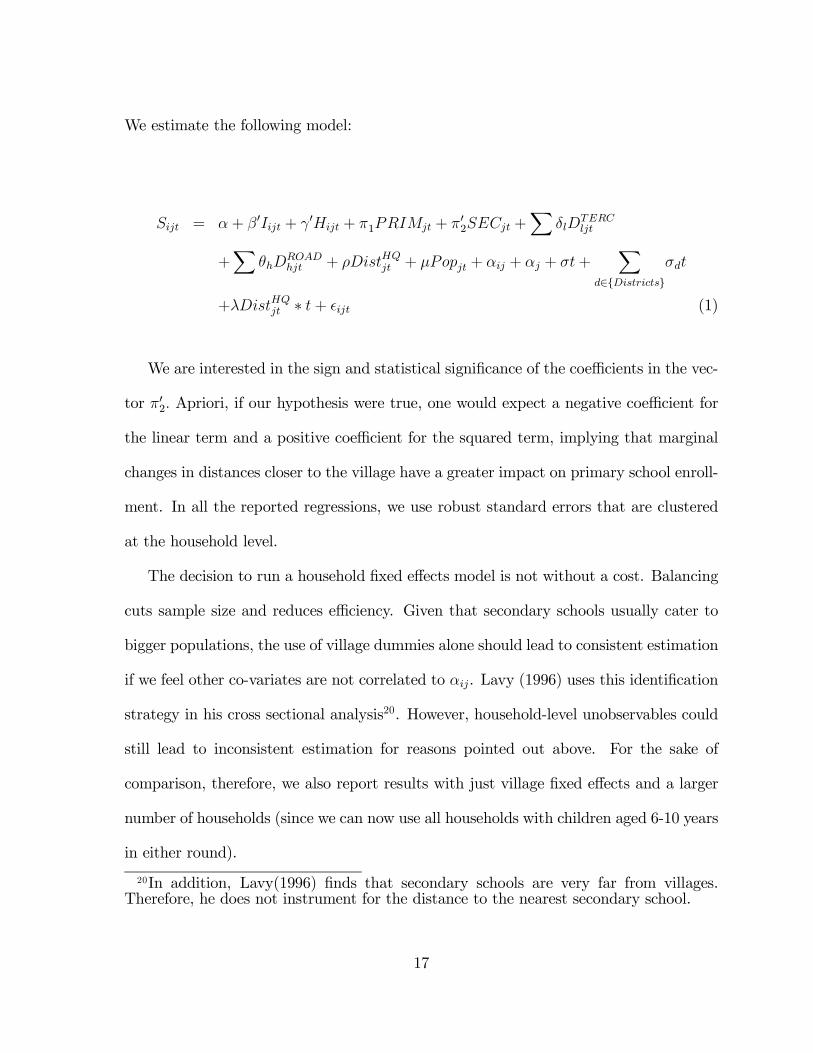
We estimate the following model:

Sijt = α + β′Iijt + γ′Hijt + π1PRIMjt + π

′2SECjt +

δlD

TERCljt

+

θhDROADhjt + ρDistHQjt + µPopjt + αij + αj + σt+

d∈{Districts}

σdt

+λDistHQjt ∗ t+ ϵijt (1)

We are interested in the sign and statistical significance of the coefficients in the vec-

tor π′2. Apriori, if our hypothesis were true, one would expect a negative coefficient for

the linear term and a positive coefficient for the squared term, implying that marginal

changes in distances closer to the village have a greater impact on primary school enroll-

ment. In all the reported regressions, we use robust standard errors that are clustered

at the household level.

The decision to run a household fixed effects model is not without a cost. Balancing

cuts sample size and reduces efficiency. Given that secondary schools usually cater to

bigger populations, the use of village dummies alone should lead to consistent estimation

if we feel other co-variates are not correlated to αij. Lavy (1996) uses this identification

strategy in his cross sectional analysis20. However, household-level unobservables could

still lead to inconsistent estimation for reasons pointed out above. For the sake of

comparison, therefore, we also report results with just village fixed effects and a larger

number of households (since we can now use all households with children aged 6-10 years

in either round).

20In addition, Lavy(1996) finds that secondary schools are very far from villages.Therefore, he does not instrument for the distance to the nearest secondary school.

17

4 Main Results

While columns (1) and (2) in Table 1 report results with household fixed effects, columns

(3) and (4) present a comparison using only village fixed effects. Results using column (1)

and (2) show that while distance to primary school has no effect, distance to secondary

schools does. The relationship is negative but the marginal impact of a drop in distance

is less at large distances. This implies that the marginal effect of a one kilometer decrease

in distance to secondary school on the share of children enrolled, evaluated at the mean

distance in 2007-08 (3.44 km), is 0.063. The marginal effect on attendance is slightly

lower at 0.060. The insignificance of distance to primary school for both variables for

this sample is not surprising because most villages already had a primary school nearby

even in 1997-98, as shown earlier.

Everything else turns out insignificant, barring the third tercile of primary school

quality (in the case of enrollment), the share of proportion of adult members doing

off farm labour, road access variables and the time trend (for attendance). We find

that a primary school of the highest quality (relatively speaking) in a village increases

the share of enrollment by 0.247 but has no impact on attendance. We find that a

unit increase in the percentage of adult members in off farm employment raises both

enrollment and attendance by 0.004. We find that a better road increases the probability

of both enrollment and attendance, though this increase is highest for paved roads21.

The insignificance of the rest of the variables could be driven by low temporal variation.

Besides, creating the balanced panel required dropping households and led to inefficiency.

21While all weather roads (Pucca) comes out to be significant for attendance, theirmagnitude is less than that for paved. This is slightly puzzling; it could be caused by aslight misclassification between paved and "pucca".

18

Therefore, that our result on secondary schooling is obtained despite this inefficiency

suggests that this effect is strong.

How do our results compare when we include only village fixed effects and include all

households that have children in either survey? The results that correspond to distance

to the nearest secondary school still survive, though they are muted. The marginal ef-

fect is again negative and decreasing in distance. The marginal effect on enrollment of a

kilometre drop in distance to the nearest secondary school is 0.040 (evaluated at mean

distance of 3.44 km) whereas the marginal effect is 0.034 for attendance. This underes-

timates the effect of distance to secondary schools and suggests the need for controlling

for household-specific fixed effects. Other significant results include the important role

of a literate mother (marginal effect of 0.059 for enrollment and 0.071 for attendance),

a literate household head (a marginal effect of 0.14 for both variables) and female head

of the family (0.108 for enrol). We also find that a greater proportion of children from

households with more land are likely to both enrol in and attend primary school (a

marginal effect of 0.007). As before, the share of off-farm employment plays a positive

role in both enrollment and attendance. Similarly, dummy variables for road access are

positive and significant for both enrollment and attendance22.

5 Robustness

In this section, we subject our specification to robustness checks. First, we want to know

if any endogeneity in secondary school placements is driving our result. We address this

22A pure pooled Ordinary Least Square estimation with no village level fixed effectsyields many more significant variables. However, insofar as our results on access to sec-ondary schooling survive all specifications, we do not forsake the fixed effects estimationmodels.

19

by running a 2 SLS estimation procedure. Second, we consider the implication of running

the regression at the child level instead of household level. Third, we test if our results

are affected by measurement errors and outliers.

5.1 Instrumental Variables

Even with individual and village fixed effects, one could contend that secondary schools

come up endogenously. We take this into account using three instruments. First, as

discussed already in Section 2, the state government of UP promoted opening up of

girls only secondary schools in blocks (administrative units which include many villages)

where there was no single sex secondary school for girls. The state government provided

a one-time infrastructure grant of one million rupees. However, these were fee-charging

schools with no aid from the government for paying salaries or incurring any other

recurrent expenditure. Due to poor initial uptake by girls, the owners of the schools,

opened under this scheme, demanded, that they be allowed to admit boys as well.

Initially, in 1999, all schools opened under these schemes were allowed to admit boys by

an executive office order, which was later revised after a gap of two years. Under the

revised order, only those schools that were located in rural areas were allowed to admit

boys along with girls. Hence, for our rural sample, the policy implied a greater access

to both boys and girls. Therefore we consider the dummy variable indicating whether

there was a girls only secondary school in the block at the baseline (Girls_School) and

interact it with time to use it as an instrument for measuring distance to secondary

school. We plausibly assume that apart from its effect through access to secondary

education, presence of girls secondary school in the block has no additional effect on

20

primary school enrollment and attendance23. Moreover, the 10th five year plan laid

emphasis on opening up new secondary schools in SC/ST concentrated areas. Hence we

use proportion of households belonging to SC and ST category in the village in 1997

(SCST_Prop), interacted with time, as the second instrument24. In addition, following

Lavy (1996), we also use changing distance to other institutions of development as

another instrument25. We construct an index variable by principal component analysis:

distance to the nearest telephone booth, police station, public distribution shop and

bank (Distance_Infrastructure)26. The implicit assumption is that improving access

to village facilities is correlated with opening secondary schools but have no incremental

impact on schooling decisions once we have controlled for other regressors.

We have a linear and a square term of distance to secondary schools that are poten-

tially endogenous. Given our three instruments, our model is over identified. We carry

out overidentification test and the result confirms the validity of the instruments (Table

2). The Hansen J Statistic is 0.654 (p-value 0.419) and 0.032 (p-value 0.858) respectively

for enrollment and attendance regressions. Thus, we fail to reject the null hypothesis

that the instruments are uncorrelated with the error term and thus validly excluded

from the estimating equation.

In the case of both attendance and enrollment, we get the same qualitative re-

23We test this further in the next section by taking into account other trends that maybe correlated with secondary school placement.24The 10th five year plan laid emphasis on providing better access to both primary

and secondary schools. However, given that primary schools were already very close tovillages in our baseline sample, we assume that this policy could have made an impactonly for secondary schools.25Lavy (1996) used distance to public telephone and post office as instruments for

distance to middle school.26It may be argued that access to telephone booth is not very relevant with the advent

of mobile phones. Our results do not change when we drop this from the index.

21

sult2728(Table 2). The linear term is negative and the square term is positive, thus

replicating the same relationship. Moreover, they are both significant in the enrollment

regression. For attendance, while the square term is significant, the linear term is almost

significant at 10% (p-value is 0.102). Reassuringly, the magnitude of the effect is very

similar for enrollment. The marginal effect at the mean for 2007-08 is now 0.060 (as

compared to 0.063 in the household fixed effects model) and 0.049 for attendance (as

compared to 0.060 in the household fixed effects model).

Given these coefficients, our qualitative results, highlighting the importance of access

to secondary schools, goes through. For both enrollment and attendance, the marginal

effect of a change in distance to secondary school using fixed effects and instruments is

similar to that obtained using just fixed effects.

5.2 Additional Trends

In this section, we check the robustness of our results by taking into account additional

trends that may be correlated with both the demand for schooling and placement of

schools. As shown in the earlier section, secondary schools came up in places where

prior educational attainment was lower. Hence, there may be differential trends in de-

27First stage results show that for both the linear term and the quadratic term, thereis a positive coefficient for Girls_School, a negative coefficient for SCST_Prop, and apositive coefficient for Distance_Infrastructure (Appendix Table A4). The first stageresult reconfirms that the increasing proximity of secondary schools has been more inblocks where there was no girls secondary school earlier, and in places with relativelymore SC/ST population. The positive relation between distance to secondary schooland the distance (index) to other infrastructure facilities (not relating to education) isalso intuitive. The F stats for the overall fit of the two first stage regressions are 20.51and 36.69.28If we include the instruments as regressors in the main equation, they come out

insignificant. While this evidence of no direct effect of instruments on the dependentvariable is flawed (though popular in the literature), it suggests that the results are notdriven by secular improvements in the village infrastructure.

22

mand for schooling depending on the initial level of educational attainment. The effect

of proximity of secondary schools on primary school enrollment can be overestimated

if villages with lower base-level education experience higher growth in both demand

for and supply of schooling. Therefore, we construct a village-level variable from the

1997 data, considering the proportion of children in the age group of 11-15 years who

have completed primary education. Since this cohort should have already finished pri-

mary schooling at the time of the baseline, it is a pre-determined variable reflecting the

baseline demand for education in the village. We interact this variable with time and

include it in the regression. Thus, the villages are allowed to follow different trajectories

depending on their baseline demand for schooling. Similarly, one can argue that the

growth in enrollment and attendance rate over time itself may vary with caste with the

less privileged castes showing a greater increase in demand for education. We take this

into account by including additional time trends which vary with the caste and religion

of the households.

The inclusion of these trends also helps us allay some apprehensions we may have

about the instruments used in the previous section. For example, it may be that the

blocks, where girls only schools did not exist in 1997, experienced a greater change in

demand for primary schooling: a pure base effect. Hence, as an additional exercise, we

run 2 SLS regressions including the village level baseline education trends (described

above). Moreover, we also include the caste and religion trends. The former ensures

that the greater access to secondary schools in areas with larger proportion of SC/ST

households in the village does not pick up the effect of an increase in demand for schooling

by these marginalized communities.

After controlling for these additional trends in the regression, we still find significant

23

negative effect of distance to secondary school on primary level enrollment and atten-

dance. The results for household fixed effects regressions, both without instruments

(OLS) and with instruments (2SLS), are reported in Table 3. The magnitude of the

effects in this specification are in line with our main specification.29 Given the evidence

from the last two sections, we report fixed effects estimation of the main specification in

the rest of the paper30.

5.3 Unit of Analysis

So far, the results obtained from household-level analysis have supported our hypothesis

that access to secondary schooling does play a significant role in determining primary

school participation. To further examine the robustness of these results, we conduct

child level analysis with household fixed effects. Hence the unit of observation becomes

specific to a child instead of a household. The dependent variable is binary enrollment

or attendance. We follow the specifications similar to our household fixed effects regres-

sions, except that we allow for child level variables like age and gender. We estimate

a linear probability model31 and use the data on all households which have children in

6-10 age group in any round32. The results show a significant negative coefficient of

distance to secondary school variable and a significant positive coefficient of its square

29The trends based on caste and religion of the households are not significant. Whilethe trend interacted with baseline demand for education is found to be negative andsignificant for enrollment (OLS), it does not affect, significantly, the coefficient of SECand SEC2.The coefficient of SEC is insignificant for Enrollment with 2SLS. Howeverthe sign is negative and SEC2 is postive and significant, as in all other specifications.30Most of our results go through even with instruments. (Results available on request)31The results go through even if we run a probit model with this specification (results

are not presented here).32The results go through even if we consider only the balanced panel of households

present in both the rounds for the child-level analysis.

24

term (Table 4). The marginal effect of a 1 km-reduction in distance to secondary school

is 0.062 on enrollment and 0.059 on attendance (evaluated at the mean distance of 3.7

in 2007-08). These results are very similar to those obtained when we use variables at

the household level.

5.4 Measurement Error and Outliers

While we have made special efforts to verify distances to nearest schools, distances could

still be reported with error33. To check whether measurement error in distances causes

inconsistency, we estimate the household fixed effects models with distance dummies

instead of distances. We define distance dummies for distance to secondary schools. We

find that the results are robust to smoothing of distance using dummies (Table 5). If the

nearest secondary school is at a distance of 1 to 5 km, then it reduces enrollment by 0.525

as compared to when it is within 1 km. The impact is around -0.40 for distances beyond

5 km (relative to there being a secondary school within 1 km of the village)34. The effect

on attendance is slightly larger at -0.608 and -0.410 for the two distance dummies.

In small datasets, large outliers often tend to drive results. To remove the impact of

outliers, based on our model, we remove observations that have residuals greater than

one standard deviation of the estimated residuals. Results stay robust to removal of

these observations and are available on request.

33We have verified distances using a village survey and by putting the same questionto households. In most cases, the distances reported in the village survey are the sameas the modal value of the distances from the household surveys for the village.34However, we find that the coefficient of dummy variable for 1-5 km is statistically

not significantly different from the coefficient of the dummy variable for greater than 5km.

25

6 Other Pathways

Next we conduct two exercises to rule out the possibility of other explanations for the

results obtained.

6.1 Secondary Schools or Secondary Education

In this paper, we check the hypothesis that the possibility of completing secondary

education affects the decision to enrol and attend school at the primary level. So far,

we have shown that access to secondary school affects primary school enrollment and

attendance. However, many secondary schools have classes 1 to 5. Secondary schools

usually have better infrastructure than stand-alone primary schools. It may be that

children go to a secondary school for their primary education as one comes up closer. In

this case, our results would give further evidence, indirectly, to the importance of better

quality.

To extricate the impact of the possibility of continuation to secondary education,

we follow another strategy. We define another dependent variable: the proportion of

household children aged 6-10 years who go to a school within the village. Further, we

use a sub-sample of villages that do not have a secondary school within two kilometers

in both periods35. In this scenario, if a larger proportion of children go to schools within

the village, this cannot be the outcome of their going to a secondary school because there

are none in the village (or even within a two kilometer radius of the village)36. In this

35This selection is based on distance, an independent variable. Therefore our estimatorsare still consistent.36Since this information is based on self-reported responses and households are not

always sure about the boundary of villages, we choose the two-kilometre radius to reducethe chances of error.

26

case, the marginal effect on primary school enrollment must be driven by the perception

that students can continue to secondary level. This is indeed the case (Table 6).

The marginal impact on the share of enrollment in the village primary school from

a reduction in distance to secondary school turns out to be 0.026 (the mean distance

to nearest secondary schools is 5.4 for such villages in 2007-08). In the case of share of

attendance in the local village school, this impact is 0.055. Thus, for villages which do

not have secondary schools, there has indeed been a considerable impact of secondary

schools opening near the village and, given that we only look at children studying inside

the village, this effect can only be due to an increased awareness of the possibility of

availing secondary education.

6.2 Sibling Externality

Participation in primary school may have improved because children have elder siblings

who have had better access to secondary schooling and are better educated. Their

elder siblings may be teaching them and motivating them to attend primary school.

If this is true, then it establishes another pathway through which access to secondary

school may be important for primary schooling. However, our objective is to check

if the proximity of secondary school has any direct impact on the primary schooling

decision despite its effect through this channel. Therefore, we run the regression model

introducing a new household level co-variate that captures the number of children in

the 14-18 age group enrolled in secondary or higher school. The results show that even

after we control for the elder sibling effect through this new variable, the distance to

secondary school and its square term both remain significant (Table 7). The magnitude

27

of the effects remains almost unchanged. It is important to note here that we recognize

the possibility that decisions regarding primary and secondary schooling of children are

determined simultaneously in a household. However, our objective is not to estimate the

causal effect of siblings; rather, we seek to show that our main results remain unperturbed

even if we account for a possible correlation between the education of primary school

age children and their older counterparts.

7 Heterogeneity of Effects

In this section, we investigate the heterogeneity of impact of access to secondary schools.

To begin with, we investigate if the impact of better access to secondary schools varies by

the size of the village. We define small villages as ones where the number of households

are less than 200 in the base year and large villages where the households are more than

20037. We find that the marginal effect of a decrease in the distance to secondary school

is positive for both small and large villages (Table 8). However, the impact of closer

secondary schools is more prominent on small villages than on large ones. A unit drop

in distance to secondary schools raises the share of enrollment rate by 0.119 and the share

of attendance by 0.164. But the marginal effects in large villages are much smaller: 0.046

and 0.050 respectively for enrollment and attendance. These larger marginal effects for

smaller villages reassure us that our results are not driven by the opening of secondary

schools in response to absolute size of demand. Rather, smaller villages were further

off from secondary schools in the base year and, therefore, have the most to gain from

changing proximity to secondary schools.37We run separate regressions for the two classes of villages as all coefficients may be

very different across the two classes.

28

We investigate whether the impact of access to secondary schools varies with trans-

port infrastructure by using a formulation where we interact a dummy variable that

measures if there is a bus stop within 1.5 km radius of the village (BUS) with the dis-

tance to the nearest secondary school38. We find that the effect of a decrease in distance

is increasing if there is a bus stop (Table 9). The marginal impact of a reduction in

distance if there is a bus stop is 0.10 on enrollment (0.114 for attendance) and 0.063

(0.060 for attendance) when there is no bus stop. This result makes sense since the

distance to the nearest secondary school measures the perception of how difficult it is

to get to the next level of schooling. Insofar as most children would need a bus to go

to these schools, our results point out that the impact of continuation kicks in when

there is a complementary bus service. It therefore points out the need for developing

infrastructure to reap these benefits.

Economic theory suggests that the effect of access to secondary schools should vary

with wealth. It is likely that a change in access cost will have a larger effect on poor

households. To check if this is indeed true, we carry out the regression separately for

households whose landholding in 1997 was below the median level and for the ones

above it. The results suggest that while we get significant effects for both groups,

the magnitude is higher for households below the median level of landholding (Table

10). The marginal effect of a one kilometer decrease in distance - on enrollment - for

poorer households (evaluated at three kilometers, the mean of the sample in 2007-08) is

38In most regressions, we stratify our regressions by variables defined at the base year,However, in the case of access to bus stop, we use an interaction term. The logic for thisis that while village size classifications are sticky over time (small villages remain smallin both periods), access to bus stop is not and changes over time. Hence, conditioningon the access to bus stop in the base year may not correctly reflect reality in the latteryear.

29

0.075 (for attendance: 0.065). The corresponding marginal effect for richer households

(evaluated at the sample mean of 3.9 km) is lesser at 0.039 (0.049 for attendance). This

result is intuitive as the cost of continued schooling binds most for poorer households.

Hence the impact of reduction in distance must be higher for them39.

Empirical studies have often cited a strong connection between health and education

(Miguel and Kremer, 2003). In our data set, we do not have anthropometric information

on children for 1997-08. In the absence of that, we use the immunization record of

households for children aged 0-5 collected in 1997-0840. We divide the households into

two groups: those where all the children in the relevant age group were immunized and

those where all the children were not immunized. We find that in households where all

children were immunized, the marginal effect of a unit decrease in distance on enrollment

(evaluated at the sample mean of 3.6 km) is 0.071 where as that for households where

all children were not immunized (evaluated at the sample mean of 3.5 km) was 0.021

(Table 11). The difference in the effect on attendance is even larger. The marginal effect

is 0.073 for the households where all children were immunized where as it is 0.009 in

the case of the other group. This difference may have two linked explanations. First,

households where all children were immunized may have a higher preference for health.

And since preference for health and education are often linked, the higher marginal

39It would have been interesting to look at the impact of decreasing distance of sec-ondary schools for various social groups. However, because of the small sample size,we are not able to run a household fixed effects regression for the General Category.The households in our sample are primarily from Scheduled Castes and Other BackwardCastes in rural Uttar Pradesh (representative of the composition of the region). Whenwe run our regression on this sub-sample, the average partial effect of a unit reductionin the distance to nearest secondary school on enrollment of the primary school goingchildren in the backward communities is found to be 0.066 (results available on request).40The survey asks if the children received any immunization, for example, for Polio,

DPT, Measles.

30

effect for these households may reflect that. A second plausible reason could be that the

health of children in households which have traditionally immunized children is better.

Therefore, they respond to changes in education opportunities better than those whose

health is not as good. This indicates an interesting link between health and educational

investment.

To investigate the heterogeneity for child level variables, we turn to child level re-

gressions. We have observed above that the overall results do not change whether we use

household as unit of analysis or children. However, for this part, child level regressions

help us investigate the heterogeneity with respect to child level variables.

We decompose the sample into two age groups, 6-7 years and 8-10 years, to see

whether the effect of secondary schooling has been more on the younger children or

the older ones. Access to secondary schooling affects the two groups differently and

the impacts on attendance and enrollment are different (Table 12). The effect of a

one kilometer decrease in distance to secondary school on enrollment is larger for the

younger age group (marginal effect of 0.14) than for the older age group (marginal effect:

0.045). For the younger children, both the linear and square terms are not significant

for attendance. However, for the older children, the effect on attendance is found to

be significant and higher: the marginal effect of a unit drop in distance to secondary

school is 0.05. These results are consistent with our stated hypothesis. Households

making decisions on whether to send their six year olds to primary school may not find

it optimal to do so if they perceive that it is unlikely that the child will be able to go to

secondary school, a level where there are economic returns. Once the child is not sent to

school in his initial years, it is less likely that he/she will be enrolled in a primary school

at a later age (8-10 years) in response to change in access to secondary school. Hence,

31

the effect on enrollment is larger for the younger age group. The results on attendance

suggest that the older age groups start to lose interest and attend school less if there

is no possibility of future continuation. This may explain their subsequent dropping

out and why many children stop going to school when they get older, despite higher

enrollment rates for younger age groups.

Next, we examine if the effects vary by gender. While distance to secondary schools

affects enrollment for boys, there are no effects for girls (Table 13). This differential

impact has two explanations.

First, recall that we hypothesize that the effect of secondary schooling comes from

the possibility to earn economic returns after schooling. However, in rural areas, it is

less likely for educated women to seek jobs41. Therefore, the effect of continuation seems

to be restricted to boys. Second, it is possible that distances to secondary schools are

still far, although they have gone down. It is well known that parents do not send girls

too far from the village. Therefore, it may be the case that the distances are such that

this effect has not kicked in for girls.

8 Extending Hypothesis to a Nationally Represen-

tative Survey

It may be contended that our results are specific to the small part of India that our

sample represents. Therefore, in this section, we provide additional evidence that sug-

gests that our (qualitative) results are general. We do so by analyzing the same effect

41This was also pointed out by Hazarika (2001).

32

using a cross sectional sample for rural India collected by the National Sample Survey.

The National Sample Survey Organization (NSSO) conducts nationally representative

household surveys on "participation and expenditure in education" once in 10 years. We

use the most recent education survey (64th round) by NSSO conducted in 2007-0842.

Detailed information about the schooling status of each child in a household is reported

in the dataset. The dataset also contains standard socioeconomic characteristics of the

household. Crucial to the paper, it contains information on key variables of interest: dis-

tance to the nearest primary, upper-primary and secondary school for each household.

This information allows us to examine the relationship between distance to the nearest

secondary school and primary school participation.

Consistent with the analysis above, we restrict our analysis to children aged 6-10

years. The average share of children enrolled in a household is 89.7 percent while the

average attendance share is 89.5 percent43. The access to secondary schooling is hetero-

geneous across rural India44. While 30.79 percent of the households have a secondary

school within 1 km, for 17.08 percent of the households the nearest secondary school is

located at a distance of more than 5 km.

Analogous to the analysis above, we regress the proportion of children enrolled (at-

tending) on individual characteristics (averaged at the household level): Age, Age2,

42Unlike in 64th round, the earlier NSSO education surveys did not have informationon distance variables for post-primary schools. Therefore, only a static cross-sectionalanalysis is possible using the NSS data.43The estimated enrollment rate for these children at the all India level (rural) is 89

percent; (boys: 90.36 percent, girls: 87.42 percent). Attendance rates do not differ muchfrom the enrollment figures: overall it is 88.76 percent (boys: 90.18 percent, girls: 87.12percent).44NSS data validate our claim that a majority of the population have easy access to

primary schools. The nearest primary school is at a distance less than 1 km for 91.88percent of the households.

33

share of male children: MALE; household characteristics: A dummy variable represent-

ing whether the household head is literate: HH_LIT, a dummy variable representing

whether the household head is female: HH_FEM, household size, dummy variables

representing land categories, dummy variable representing whether the household is

a Muslim: MUSLIM, dummy variables representing social groups, distance dummy

variables for primary school (PRIM) and secondary school (SEC)45. We control for

sub-regional differences by using dummy variables. While the attempt has been to keep

the same set of variables as the analysis above, we are constrained by the variables

available in the data set. For example we cannot control for the quality of the village

primary school or any other access variable.

It is important to begin by the remark that the results should be treated as only

suggestive. Given the cross sectional nature of data, we do not make any claims on

causality. Indeed the earlier part of our paper shows the importance of the panel struc-

ture. The results here are provided to indicate that the results from the previous section

are not specific to our sample but are consistent with correlations observed in a nationally

representative sample.

We provide two sets of results in Table 14. The first column corresponds to the

proportion of children in the 6-10 age group enrolled in school and the second column

to the proportion of children in the 6-10 age group who attend school. We do not

focus as much on other variables but their results are as expected46. Moving to the

45The distance categories are specified in the National Sample Survey.46We find that age (Age) has the usual increasing and concave relationship with enroll-

ment. Since some children start school late, more children are found enrolled in schoolas one raises the age at initial induction ages. However, after a certain age, they aremore likely to drop out. The proportion of males among children (Male) is positive andsignificant, hinting that the gap between boys and girls in primary schooling still exists.Among household level variables, we find that the presence of a literate head increases S

34

variables of interest, we find that distance to primary schools is still an important co-

variate of enrollment and attendance. Despite schemes that target primary schooling,

including massive investment in school infrastructure, this result points to the need

for more primary schools. We find that if the primary school is between one and five

kilometers away, the proportion of children enrolled falls by 1.6 percentage points than

when primary schools are less than one kilometer away. This proportion falls by 17

percentage points if primary schools are more than five kilometers away. In this case,

the affect on attendance is even more with a 19.2 percentage fall as compared to the

reference access category. This result is different from the result from our sample since

there is more heterogeneity in the all India sample.

Next we turn to the results for distance to secondary schools. We find that secondary

schools have no discernible differential impact on primary schooling if they are at a

distance of one to five kilometers than when the school is within a one kilometer radius

(the reference category). However, if secondary schools are more than five kilometers

away from the household, then this is associated with a 2.5 percentage-point lower share

of enrolled children. This seems to indicate a link between secondary schooling and

primary education enrollment. This negative partial correlation between distance to

secondary schools and enrollment/ attendance is a strong indication that our hypothesis

by 11 percentage points while the presence of a female head increases the proportion by2.4 percentage points. Households with greater land ownership have higher enrollment,pointing out that richer households are more likely to send children to school despitefree education. Households with land ownership of 0.05 to one acre have 3 percentagepoints higher proportion of children enrolled than households with less than 0.05 acreof land (the reference category). Households with more than one acre of land have 5percentage points higher proportion of children enrolled in school as compared to thereference category. A greater household size, reflecting a squeeze on household resources,causes a lower share of enrollment. Muslims households have 7 percentage points lesserchildren enrolled in households than other religious groups. Schedule tribes are the leastlikely to be enrolled in school, with the smallest S, followed by Schedule Caste who have3.9 percentage points lesser S than the reference category (General caste).

35

may hold for most of rural India.

9 Conclusion

Universal primary education has been a stated aim of development policy experts as

well as of governments. Policies to improve outcome for primary education have largely

focussed on access to primary schools. In recent years, this emphasis has moved to

quality of education with efforts being made to improve the quality of teachers. However,

a key component that drives the decision of households to send children to school is the

economic returns to schooling. This paper builds on recent work in the literature on

the economics of education that shows that the perceived (real, in many cases) returns

to education are convex. We posit that if this is true, it is plausible that education

investment is lumpy - that to elicit profitable returns from education, households have

to invest in their child’s education until they pass high school. Households take into

account the cost of post-primary schooling in making decisions at even the primary level.

Amajor component of the cost of post primary schooling is distance to secondary schools.

This paper explores whether access to secondary schools affects primary schooling.

We estimate the significance of the hypothesized relation using a panel data set on

households from 43 villages in Uttar Pradesh, a state in India where primary schooling

is far from universal. Taking advantage of policies that led to equalization of access to

secondary schooling, we find that the distance to the nearest secondary school is indeed

a significant determinant of primary school enrollment and attendance. The marginal

effect on the proportion of children in a household enrolled in a primary school, from a

one kilometer decrease in distance to secondary school, evaluated at the mean distance

36

in 2007-08 (3.44 km) is 0.063. The marginal effect on attendance is slightly lower at

0.060.

Further, to test whether our results are driven by endogenous placement of secondary

schools, we run a 2 SLS estimation using the block level variation in presence of girls

secondary school at the baseline, proportion of SC/ST households in the village at

the baseline, and an index of access to infrastructure facilities (that do not directly

affect schooling) as instruments. The choice of the first two instruments are motivated

by national and state level educational policies in effect during the period of study.

Changing access to infrastructure (in the spirit of previous research by Lavy, 1996) is

also used as an instrument, although the results do not change if we drop this instrument.

We find that our results are robust to instrumentation.

Next, our paper also finds that the impact of secondary schools in the vicinity is

driven by the possibility of continuation and not merely because secondary schools may

provide better quality education at the primary level. In villages that do not have

secondary schools, the marginal impact on the share of enrollment in the village primary

school from a reduction in distance to secondary school turns out to be 0.026 (the mean

distance to nearest secondary schools is 5.4 for such villages in 2007-08). In the case of

share of attendance in the local village school, this impact is 0.055. This suggests that

the effect on primary schooling outcomes is driven by continuation possibilities. We also

rule out the possibility of other pathways confounding the effect. For example, it is not

the case that the effect disappears if we account for the fact that children studying in

secondary schools mentor their younger siblings to go to primary schools.

We find that the impact of secondary schools is heterogeneous. The impact is greater

when there is a complementary bus stop close to the village and the smaller the villages in

37

the baseline survey, the greater the effect. We find that households that lie in the bottom

half of the baseline land distribution are affected more. We also find that households

that have immunized all their children react more to the decrease in distance. This

suggests that the ability to respond to better schooling opportunities depend on health

outcomes of children. Interestingly, we find that the effect is larger for enrollment of

children aged 6-7 years; however, for the children aged 8-10, the effect is larger for their

attendance. We find the effect is larger for boys than for girls. This is again consistent

with our hypothesis since work participation rate among men is larger than for women.

So men are more likely to reap economic benefits from reaching secondary schools.

While these results are obtained for a sample of 43 villages in a poor part of India,

our hypothesis may be much more general. Despite the omission of some key variables

in a nationally representative survey (National Sample Survey 2007-08), we run a sim-

ple regression to show that there is a negative correlation nationally between access

to secondary schools and primary schooling enrollment (and attendance). Controlling

for distance to primary schools, we find that if secondary schools are more than five

kilometers away, there is a 2.5 percentage-point decrease in share of primary enrolled

children.

In light of these results, our paper suggests that access to post-primary schools is

important for meeting primary schooling objectives. While on the one hand it can be

argued that secondary schools will open up privately as soon as enough children are

primary educated, this critical mass of primary educated children may never develop

in many parts of the developing world. In the absence of continuation possibilities,

households may pull their children out of primary schools. Thus, all levels of schooling

need to be developed and accessible at the same time to achieve universal education.

38

References

[1] Andrabi, Tahir, Jishnu Das and Asim I. Khwaja (2013), "Students Today, Teachers

Tomorrow: Identifying constraints on the provision of education", Journal of Public

Economics, 100, pp 1-14.

[2] Banerjee, Abhijit and Esther Duflo (2005), "Growth Theory through the Lens of

Development Economics", in P. Aghion and S. N. Durlauf (eds.) Handbook of Eco-

nomic Growth, 1A, North-Holland, Amsterdam, pp 473-552.

[3] Banerjee, Abhijeet and Esther Duflo (2011), Poor Economics: A Radical Rethinking

of the Way to Fight Global Poverty, PublicAffairs, United States.

[4] Bommier, Antoine and Sylvie Lambart (2000), "Education Demand and Age at

School Enrollment in Tanzania", The Journal of Human Resources, 35(1), pp 177-

203.

[5] Brown, Philip H. and Albert Park (2002), "Education and poverty in rural China,"

Economics of Education Review, 21(6), pp 523-541.

[6] Burde, Dana and Leigh L. Linden (2012), "The Effect of Village-Based Schools:

Evidence from a Randomized Controlled Trial in Afghanistan", NBER Working

Paper No. 18039.

[7] Burke, Kathleen and Kathleen Beegle (2004), "Why Children Aren’t Attending

School: The Case of Northwestern Tanzania", Journal of African Economics, 13(2),

pp 333-355.

39

[8] Colclough, C.; G. Kingdon and H. Patrinos (2010). "The Changing Pattern of Wage

Returns to Education and its Implications", Development Policy Review, 28(6), pp

733-747.

[9] Duflo, Esther (2001), "Schooling and Labor Market Consequences of School Con-

struction in Indonesia: Evidence from an Unusual Policy Experiment", American

Economic Review, 91(4), pp 795-813.

[10] Duraisamy, P. (2002), "Changes in Returns to Education in India, 1983-94: By

Gender, Age-cohort and Location", Economics of Education Review, 21(6), pp 609-

622.

[11] Filmer, Deon (2007), "If You Build It, Will They Come? School Availability and

School Enrollment in 21 Poor Countries", Journal of Development Studies, 43(5),

pp 901-928.

[12] Glewwe, Paul (2002), "Schools and Skills in Developing Countries: Education Poli-

cies and Socioeconomic Outcomes", Journal of Economic Literature, 40(2), pp 436-

482.

[13] Glick, Peter and David E. Sahn (2006), "The Demand for Primary Schooling in

Madagascar: Price, Quality, and the Choice between Public and Private Providers",

Journal of Development Economics, 79(1), pp 118-145.

[14] Handa, Sudhanshu (2002), "Raising Primary School Enrollment in Developing

Countries: The Relative Importance of Supply and Demand", Journal of Devel-

opment Economics, 69(1), pp 103-128.

40

[15] Hazarika, Gautam (2001), "The Sensitivity of Primary School Enrollment to the

Costs of Post-Primary Schooling in Rural Pakistan: A Gender Perspective", Edu-

cation Economics, 9(3), pp 237-244.

[16] Jensen, Robert (2010), "The (Perceived) Returns to Education and the Demand

for Schooling", Quarterly Journal of Economics, 125(2), pp 515-548.

[17] Jha, Jyotsna and Ramya Subrahmanian (2005), "Secondary Education in the Indian

State of Uttar Pradesh: Gender Dimensions of State Policy and Practice", United

Nations Research Institute for Social Development (UNRISD).

[18] Kingdon, Geeta Gandhi and Jeemol Unni (2001), "Education and Women’s Labour

Market Outcomes in India", Education Economics, 9(2), pp 173-195.

[19] Kingdon, Geeta Gandhi (2007), "The Progress of School Education in India", Ox-

ford Review of Economic Policy, 23(2), pp 168-195.

[20] Kingdon, G., H. Patrinos, C. Sakellariou and M. Soderbom (2008), "International

Pattern of Returns to Education", Mimeo, World Bank.

[21] Lavy, Victor (1996), "School Supply Constraints and Children’s Educational Out-

comes in Rural Ghana", Journal of Development Economics, 51(2), pp 291-314.

[22] Lincove, Jane Arnold (2009), "Determinants of Schooling for Boys and Girls in

Nigeria under a Policy of Free Primary Education", Economics of Education Review,

28(4), pp 474-484.

41

[23] Manski, Charles F. (1993), "Adolescent Econometricians: How Do Youth Infer the

Returns to Schooling?", in C. Clotfelter and M. Rothschild (eds.) Studies of Supply

and Demand in Higher Education, University of Chicago Press, Chicago.

[24] Miguel, E. and M. Kremer (2004), "Worms: Identifying Impacts on Education

and Health in the Presence of Treatment Externalities", Econometrica, 72(1), pp

159—217.

[25] Muralidharan, Karthik and Nishith Prakash (2012), "Cycling to School: Increasing

High School Enrollment for Girls in Bihar", Mimeo.

[26] Nguyen, Trang (2008), "Information, Role Models and Perceived Returns to Edu-

cation: Experimental Evidence from Madagascar", Mimeo, MIT.

[27] Orazem, Peter F. and Elizabeth M. King (2007), "Schooling in Developing Coun-

tries: The Roles of Supply, Demand and Government Policy", in T.P. Schultz and J.

Strauss (eds.) Handbook of Development Economics, 4, North-Holland, Amsterdam,

pp 3475-3559.

[28] Pitt, Mark M., Mark R. Rosenzweig and Donna M. Gibbons (1993), "The Determi-

nants and Consequences of the Placement of Government Programs in Indinesia",

World Bank Economic Review, 7(3), pp 319-348.

[29] Psacharopoulos, G. (1994), "Returns to Investment in Education: a Global Up-

date", World Development, 22(9), pp 1325—1343.

[30] Psacharopoulos, G. and H. Patrinos (2004), "Returns to Investment in Education:

A Further Update", Education Economics, 12(2), pp 111-134.

42

[31] Schultz, T. P. (2004), "Evidence of Returns to Schooling in Africa from House-

hold Surveys: Monitoring and Restructuring the Market for Education", Journal

of African Economies, 13(2), pp ii95-ii148.

[32] Vuri, D. (2008), "The Effect of Availability and Distance to School on Children’s

Time Allocation in Ghana and Guatemala", Understanding Children’s Work Pro-

gramme Working Paper.

43

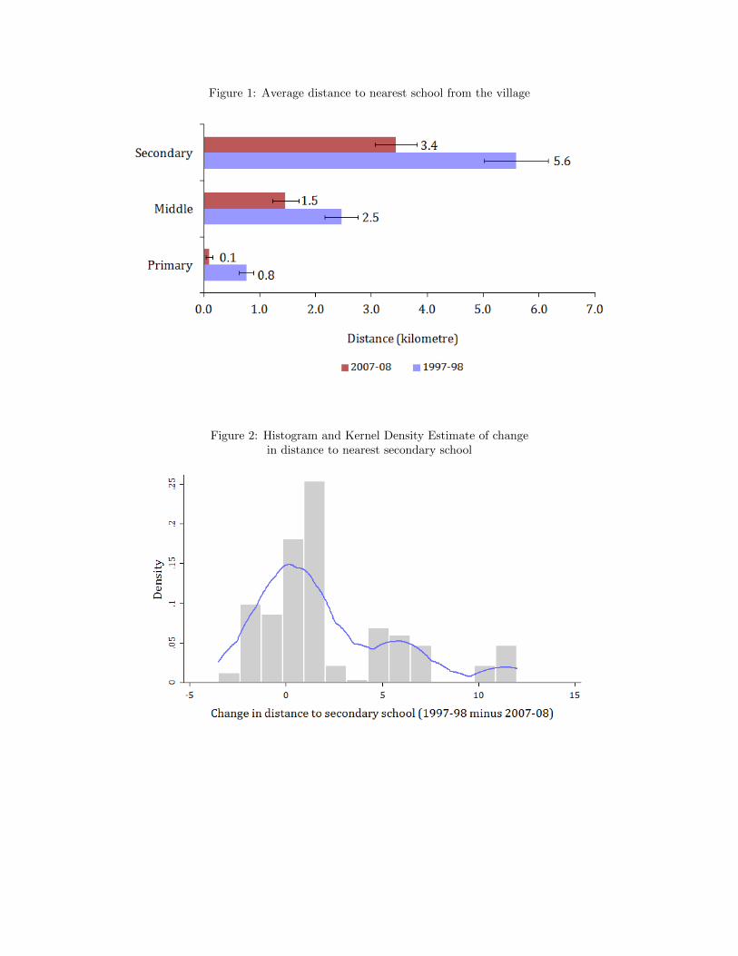
Figure 1: Average distance to nearest school from the village

Figure 2: Histogram and Kernel Density Estimate of changein distance to nearest secondary school

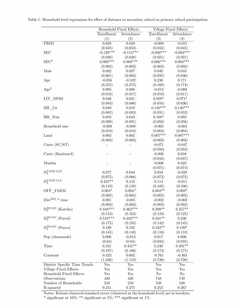
Table 1: Household level regressions for e§ect of distance to secondary school on primary school participation

Household Fixed E§ects Village Fixed E§ects

Enrollment Attendance Enrollment Attendance

(1) (2) (3) (4)

PRIM 0.028 0.049 -0.009 -0.015

(0.045) (0.053) (0.043) (0.045)

SEC -0.120*** -0.114*** -0.080*** -0.063***

(0.026) (0.028) (0.021) (0.021)

SEC2 0.008*** 0.008*** 0.006*** 0.004***

(0.002) (0.002) (0.002) (0.002)

Male 0.082 0.037 0.040 0.010

(0.061) (0.063) (0.035) (0.036)

Age -0.056 -0.102 0.230 0.171

(0.255) (0.275) (0.169) (0.174)

Age2 0.005 0.008 -0.012 -0.008

(0.016) (0.017) (0.010) (0.011)

LIT_MOM 0.046 0.031 0.059* 0.071*

(0.083) (0.086) (0.034) (0.036)

HH_Lit 0.049 0.019 0.140*** 0.140***

(0.082) (0.083) (0.031) (0.032)

HH_Fem 0.058 0.043 0.108* 0.093

(0.090) (0.091) (0.056) (0.056)

Household size -0.008 -0.009 -0.005 -0.004

(0.010) (0.010) (0.004) (0.004)

Land 0.002 0.002 0.007*** 0.007***

(0.003) (0.003) (0.002) (0.002)

Caste (SC/ST) - - -0.071 -0.047

(0.050) (0.053)

Caste (Backward) - - -0.006 0.016

(0.044) (0.047)

Muslim - - -0.006 0.023

(0.071) (0.074)

DTERCILE2 0.077 0.044 0.034 -0.028

(0.075) (0.086) (0.072) (0.072)

DTERCILE3 0.247** 0.153 0.114 -0.011

(0.119) (0.129) (0.105) (0.106)

OFF_FARM 0.004* 0.004* 0.004** 0.003*

(0.002) (0.002) (0.002) (0.002)

DistHQ * time 0.001 -0.001 -0.002 -0.003

(0.003) (0.003) (0.003) (0.002)

DROAD2 (Katcha) 0.448*** 0.462*** 0.299** 0.257**

(0.153) (0.163) (0.123) (0.125)

DROAD3 (Paved) 0.519*** 0.482*** 0.331** 0.236

(0.175) (0.185) (0.142) (0.145)

DROAD4 (Pucca) 0.198 0.192 0.242** 0.199*

(0.145) (0.148) (0.116) (0.118)

Pop (thousands) 0.006 -0.013 0.017 0.006

(0.04) (0.04) (0.034) (0.035)

Time 0.241 0.455** 0.240 0.401**

(0.197) (0.196) (0.173) (0.175)

Constant 0.423 0.602 -0.761 -0.463

(1.036) (1.119) (0.720) (0.739)

District SpeciÖc Time Trends Yes Yes Yes Yes

Village Fixed E§ects Yes Yes Yes Yes

Household Fixed E§ects Yes Yes No No

Observations 420 420 748 748

Number of Households 210 210 538 538

R-squared 0.251 0.275 0.253 0.267

Notes: Robust clustered standard errors (clustered at the household level) are in brackets.

* signiÖcant at 10%; ** signiÖcant at 5%; *** signiÖcant at 1%.

Table 2: Household level Öxed e§ects instrumental variables (2SLS) estimation

Enrollment Attendance(1) (2)

SEC -0.118** -0.101(0.059) (0.061)

SEC2 0.009** 0.008*(0.004) (0.004)

Other Covariates Yes YesDistrict SpeciÖc Time Trends Yes YesHousehold Fixed E§ects Yes YesObservations 388 388Number of Households 194 194OveridentiÖcation Test (Hansen J Statistic) 0.654 0.032(p-value) (0.419) (0.858)

Notes: Robust clustered standard errors (clustered at the household level)are in brackets. * signiÖcant at 10%; ** signiÖcant at 5%; *** signiÖcant at1%. The regressors SEC and SEC2 are instrumented by three instruments:(i) whether there was a single sex girls secondary school in the block atthe baseline interacted with time, (ii) proportion of SC/ST households inthe village at the baseline interacted with time, and (iii) village distance toinfrastructure index. The village level index for distance to infrastructureis constructed by principal component analysis of four variables: distanceto the nearest telephone service, police station, PDS and bank.

Table 3: Household level regressions controlling for additional trends

Household FE - OLS Household FE - 2SLSEnrollment Attendance Enrollment Attendance

(1) (2) (3) (4)SEC -0.111*** -0.108*** -0.102 -0.109*

(0.027) (0.029) (0.066) (0.066)SEC2 0.008*** 0.008*** 0.008* 0.008**

(0.002) (0.002) (0.004) (0.004)Baseline education * time -0.543** -0.425 -0.355 -0.090

(0.266) (0.263) (0.324) (0.303)Caste (SC/ST) * time 0.087 0.049 0.097 0.059

(0.115) (0.111) (0.120) (0.119)Caste (Backward) * time 0.053 0.066 0.089 0.116

(0.109) (0.102) (0.102) (0.101)Muslim * time 0.168 0.161 0.160 0.173

(0.163) (0.170) (0.160) (0.173)Other Covariates Yes Yes Yes YesDistrict SpeciÖc Time Trends Yes Yes Yes YesVillage Fixed E§ects Yes Yes Yes YesHousehold Fixed E§ects Yes Yes Yes YesObservations 420 420 388 388Number of Households 210 210 194 194R-squared 0.276 0.290 - -

Notes: Robust clustered standard errors (clustered at the household level) are in brackets.* signiÖcant at 10%; ** signiÖcant at 5%; *** signiÖcant at 1%.

Table 4: Child level regressions

Household Fixed E§ects Village Fixed E§ectsEnrollment Attendance Enrollment Attendance

(1) (2) (3) (4)SEC -0.122*** -0.114*** -0.080*** -0.061***

(0.032) (0.034) (0.020) (0.021)SEC2 0.008*** 0.007*** 0.005*** 0.004**

(0.003) (0.003) (0.002) (0.002)Other Covariates Yes Yes Yes YesDistrict SpeciÖc Time Trends Yes Yes Yes YesVillage Fixed E§ects Yes Yes Yes YesHousehold Fixed E§ects Yes Yes No NoObservations 1271 1271 1271 1271R-squared 0.674 0.673 0.235 0.241

Notes: Robust clustered standard errors (clustered at the household level) are inbrackets. * signiÖcant at 10%; ** signiÖcant at 5%; *** signiÖcant at 1%.

Table 5: Results with distance dummies for secondary school

Enrollment Attendance(1) (2)

SEC (1km d < 5km) -0.525*** -0.608***(0.194) (0.185)

SEC (d 5km) -0.400*** -0.410***(0.111) (0.113)

Other Covariates Yes YesDistrict SpeciÖc Time Trends Yes YesHousehold Fixed E§ects Yes YesObservations 420 420Number of Households 210 210R-squared 0.231 0.270

Notes: Robust clustered standard errors (clustered at thehousehold level) are in brackets. * signiÖcant at 10%; ** sig-niÖcant at 5%; *** signiÖcant at 1%.

Table 6: E§ects of change in secondary-school-distance outside village on primary-school-participation withinvillage

Enrollment Attendance(1) (2)

SEC -0.463*** -0.519***(0.099) (0.111)

SEC2 0.041*** 0.043***(0.011) (0.011)

Other Covariates Yes YesDistrict SpeciÖc Time Trends Yes YesHousehold Fixed E§ects Yes YesObservations 212 212Number of Households 106 106R-squared 0.331 0.318

Notes: Robust clustered standard errors (clustered at thehousehold level) are in brackets. * signiÖcant at 10%; ** sig-niÖcant at 5%; *** signiÖcant at 1%.

Table 7: E§ects after controlling for sibling externality

Enrollment Attendance(1) (2)

SEC -0.120*** -0.116***(0.026) (0.028)

SEC2 0.008*** 0.008***(0.002) (0.002)

SEC_SIBLING -0.001 0.029(0.038) (0.042)

Other Covariates Yes YesDistrict SpeciÖc Time Trends Yes YesHousehold Fixed E§ects Yes YesObservations 420 420Number of Households 210 210R-squared 0.251 0.277

Notes: Robust clustered standard errors (clustered at thehousehold level) are in brackets. * signiÖcant at 10%; ** sig-niÖcant at 5%; *** signiÖcant at 1%.

Table 8: E§ects in small and large villages

Small Villages Large VillagesEnrollment Attendance Enrollment Attendance

(1) (2) (3) (4)SEC -0.533** -0.718*** -0.065 -0.076

(0.228) (0.227) (0.047) (0.047)SEC2 0.050** 0.068*** 0.003 0.004

(0.023) (0.023) (0.004) (0.004)Other Covariates Yes Yes Yes YesDistrict SpeciÖc Time Trends Yes Yes Yes YesHousehold Fixed E§ects Yes Yes Yes YesObservations 164 164 256 256Number of Households 82 82 128 128R-squared 0.338 0.351 0.304 0.354

Notes: Robust clustered standard errors (clustered at the household level) are inbrackets. * signiÖcant at 10%; ** signiÖcant at 5%; *** signiÖcant at 1%. Small(large) villages are deÖned as villages where the number of households were less(more) than 200 in 1997-98.

Table 9: E§ect of access to secondary school depending on village access to bus stop

Enrollment Attendance(1) (2)

SEC -0.135*** -0.135***(0.028) (0.030)

SEC2 0.011*** 0.011***(0.002) (0.002)

SEC * BUS -0.038* -0.054**(0.021) (0.023)

Other Covariates Yes YesDistrict SpeciÖc Time Trends Yes YesHousehold Fixed E§ects Yes YesObservations 420 420Number of Households 210 210R-squared 0.262 0.295

Notes: Robust clustered standard errors (clustered at thehousehold level) are in brackets. * signiÖcant at 10%; ** sig-niÖcant at 5%; *** signiÖcant at 1%.

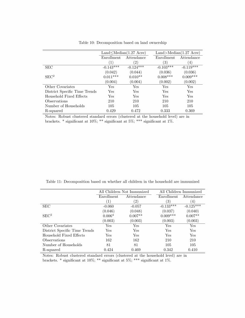
Table 10: Decomposition based on land ownership

LandMedian(1.27 Acre) Land>Median(1.27 Acre)Enrollment Attendance Enrollment Attendance

(1) (2) (3) (4)SEC -0.143*** -0.124*** -0.103*** -0.119***

(0.042) (0.044) (0.036) (0.036)SEC2 0.011*** 0.010** 0.008*** 0.009***

(0.004) (0.004) (0.002) (0.002)Other Covariates Yes Yes Yes YesDistrict SpeciÖc Time Trends Yes Yes Yes YesHousehold Fixed E§ects Yes Yes Yes YesObservations 210 210 210 210Number of Households 105 105 105 105R-squared 0.429 0.472 0.333 0.369

Notes: Robust clustered standard errors (clustered at the household level) are inbrackets. * signiÖcant at 10%; ** signiÖcant at 5%; *** signiÖcant at 1%.

Table 11: Decomposition based on whether all children in the household are immunized

All Children Not Immunized All Children ImmunizedEnrollment Attendance Enrollment Attendance

(1) (2) (3) (4)SEC -0.060 -0.057 -0.133*** -0.125***

(0.046) (0.048) (0.037) (0.040)SEC2 0.006* 0.007** 0.009*** 0.007**

(0.003) (0.003) (0.003) (0.003)Other Covariates Yes Yes Yes YesDistrict SpeciÖc Time Trends Yes Yes Yes YesHousehold Fixed E§ects Yes Yes Yes YesObservations 162 162 210 210Number of Households 81 81 105 105R-squared 0.424 0.469 0.342 0.410

Notes: Robust clustered standard errors (clustered at the household level) are inbrackets. * signiÖcant at 10%; ** signiÖcant at 5%; *** signiÖcant at 1%.

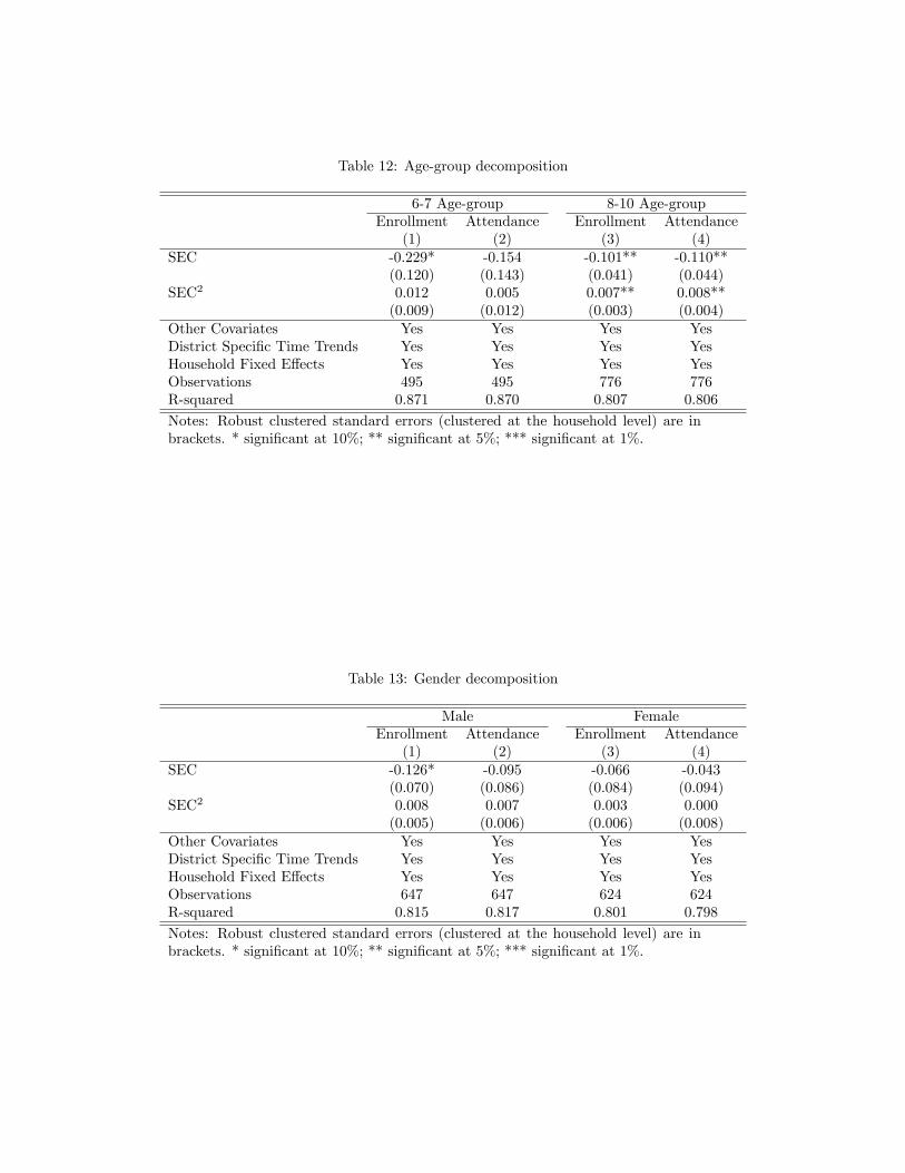
Table 12: Age-group decomposition

6-7 Age-group 8-10 Age-groupEnrollment Attendance Enrollment Attendance

(1) (2) (3) (4)SEC -0.229* -0.154 -0.101** -0.110**

(0.120) (0.143) (0.041) (0.044)SEC2 0.012 0.005 0.007** 0.008**

(0.009) (0.012) (0.003) (0.004)Other Covariates Yes Yes Yes YesDistrict SpeciÖc Time Trends Yes Yes Yes YesHousehold Fixed E§ects Yes Yes Yes YesObservations 495 495 776 776R-squared 0.871 0.870 0.807 0.806

Notes: Robust clustered standard errors (clustered at the household level) are inbrackets. * signiÖcant at 10%; ** signiÖcant at 5%; *** signiÖcant at 1%.

Table 13: Gender decomposition

Male FemaleEnrollment Attendance Enrollment Attendance

(1) (2) (3) (4)SEC -0.126* -0.095 -0.066 -0.043

(0.070) (0.086) (0.084) (0.094)SEC2 0.008 0.007 0.003 0.000

(0.005) (0.006) (0.006) (0.008)Other Covariates Yes Yes Yes YesDistrict SpeciÖc Time Trends Yes Yes Yes YesHousehold Fixed E§ects Yes Yes Yes YesObservations 647 647 624 624R-squared 0.815 0.817 0.801 0.798

Notes: Robust clustered standard errors (clustered at the household level) are inbrackets. * signiÖcant at 10%; ** signiÖcant at 5%; *** signiÖcant at 1%.

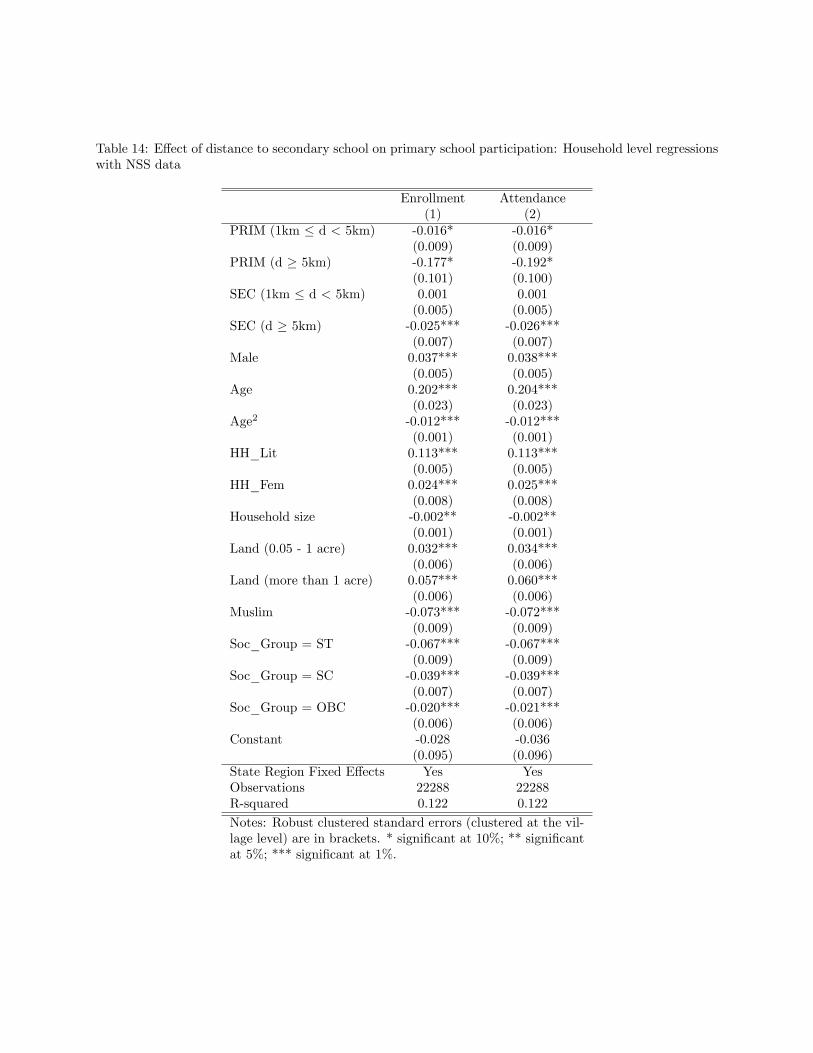
Table 14: E§ect of distance to secondary school on primary school participation: Household level regressionswith NSS data

Enrollment Attendance(1) (2)

PRIM (1km d < 5km) -0.016* -0.016*(0.009) (0.009)

PRIM (d 5km) -0.177* -0.192*(0.101) (0.100)

SEC (1km d < 5km) 0.001 0.001(0.005) (0.005)

SEC (d 5km) -0.025*** -0.026***(0.007) (0.007)

Male 0.037*** 0.038***(0.005) (0.005)

Age 0.202*** 0.204***(0.023) (0.023)

Age2 -0.012*** -0.012***(0.001) (0.001)

HH_Lit 0.113*** 0.113***(0.005) (0.005)

HH_Fem 0.024*** 0.025***(0.008) (0.008)

Household size -0.002** -0.002**(0.001) (0.001)

Land (0.05 - 1 acre) 0.032*** 0.034***(0.006) (0.006)

Land (more than 1 acre) 0.057*** 0.060***(0.006) (0.006)

Muslim -0.073*** -0.072***(0.009) (0.009)

Soc_Group = ST -0.067*** -0.067***(0.009) (0.009)

Soc_Group = SC -0.039*** -0.039***(0.007) (0.007)

Soc_Group = OBC -0.020*** -0.021***(0.006) (0.006)

Constant -0.028 -0.036(0.095) (0.096)

State Region Fixed E§ects Yes YesObservations 22288 22288R-squared 0.122 0.122

Notes: Robust clustered standard errors (clustered at the vil-lage level) are in brackets. * signiÖcant at 10%; ** signiÖcantat 5%; *** signiÖcant at 1%.

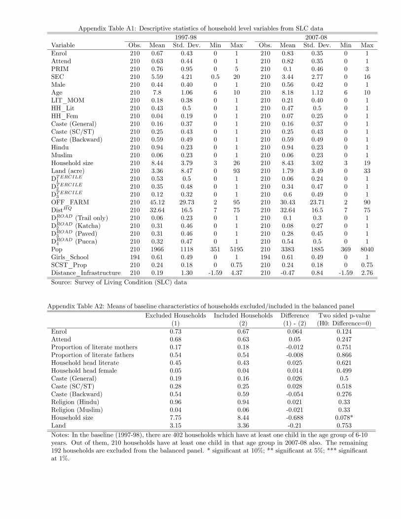
Appendix Table A1: Descriptive statistics of household level variables from SLC data1997-98 2007-08

Variable Obs. Mean Std. Dev. Min Max Obs. Mean Std. Dev. Min MaxEnrol 210 0.67 0.43 0 1 210 0.83 0.35 0 1Attend 210 0.63 0.44 0 1 210 0.82 0.35 0 1PRIM 210 0.76 0.95 0 5 210 0.1 0.46 0 3SEC 210 5.59 4.21 0.5 20 210 3.44 2.77 0 16Male 210 0.44 0.40 0 1 210 0.56 0.42 0 1Age 210 7.8 1.06 6 10 210 8.18 1.12 6 10LIT_MOM 210 0.18 0.38 0 1 210 0.21 0.40 0 1HH_Lit 210 0.43 0.5 0 1 210 0.47 0.5 0 1HH_Fem 210 0.04 0.19 0 1 210 0.07 0.25 0 1Caste (General) 210 0.16 0.37 0 1 210 0.16 0.37 0 1Caste (SC/ST) 210 0.25 0.43 0 1 210 0.25 0.43 0 1Caste (Backward) 210 0.59 0.49 0 1 210 0.59 0.49 0 1Hindu 210 0.94 0.23 0 1 210 0.94 0.23 0 1Muslim 210 0.06 0.23 0 1 210 0.06 0.23 0 1Household size 210 8.44 3.79 3 26 210 8.43 3.02 3 19Land (acre) 210 3.36 8.47 0 93 210 1.79 3.49 0 33DTERCILE1 210 0.53 0.5 0 1 210 0.06 0.24 0 1DTERCILE2 210 0.35 0.48 0 1 210 0.34 0.47 0 1DTERCILE3 210 0.12 0.32 0 1 210 0.6 0.49 0 1OFF_FARM 210 45.12 29.73 2 95 210 30.43 23.71 2 90DistHQ 210 32.64 16.5 7 75 210 32.64 16.5 7 75DROAD1 (Trail only) 210 0.06 0.23 0 1 210 0.1 0.3 0 1DROAD2 (Katcha) 210 0.31 0.46 0 1 210 0.08 0.27 0 1DROAD3 (Paved) 210 0.31 0.46 0 1 210 0.28 0.45 0 1DROAD4 (Pucca) 210 0.32 0.47 0 1 210 0.54 0.5 0 1Pop 210 1966 1118 351 5195 210 3383 1885 369 8040Girls_School 194 0.61 0.49 0 1 194 0.61 0.49 0 1SCST_Prop 210 0.24 0.18 0 0.75 210 0.24 0.18 0 0.75Distance_Infrastructure 210 0.19 1.30 -1.59 4.37 210 -0.47 0.84 -1.59 2.76

Source: Survey of Living Condition (SLC) data

Appendix Table A2: Means of baseline characteristics of households excluded/included in the balanced panelExcluded Households Included Households Di§erence Two sided p-value

(1) (2) (1) - (2) (H0: Di§erence=0)Enrol 0.73 0.67 0.064 0.124Attend 0.68 0.63 0.05 0.247Proportion of literate mothers 0.17 0.18 -0.012 0.751Proportion of literate fathers 0.54 0.54 -0.008 0.866Household head literate 0.45 0.43 0.025 0.621Household head female 0.05 0.04 0.014 0.499Caste (General) 0.19 0.16 0.026 0.5Caste (SC/ST) 0.28 0.25 0.028 0.518Caste (Backward) 0.54 0.59 -0.054 0.276Religion (Hindu) 0.96 0.94 0.021 0.33Religion (Muslim) 0.04 0.06 -0.021 0.33Household size 7.75 8.44 -0.688 0.078*Land 3.15 3.36 -0.21 0.753

Notes: In the baseline (1997-98), there are 402 households which have at least one child in the age group of 6-10years. Out of them, 210 households have at least one child in that age group in 2007-08 also. The remaining192 households are excluded from the balanced panel. * signiÖcant at 10%; ** signiÖcant at 5%; *** signiÖcantat 1%.

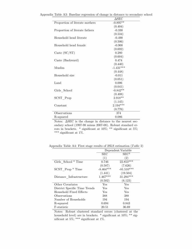
Appendix Table A3: Baseline regression of change in distance to secondary schoolSEC

Proportion of literate mothers -0.895**(0.404)

Proportion of literate fathers -0.330(0.534)

Household head literate -0.490(0.506)

Household head female -0.900(0.692)

Caste (SC/ST) 0.280(0.604)

Caste (Backward) 0.474(0.440)

Muslim -1.431***(0.448)

Household size -0.011(0.051)

Land 0.006(0.041)

Girls_School -0.842**(0.408)

SCST_Prop 2.918**(1.145)

Constant 2.194***(0.776)

Observations 374R-squared 0.086

Notes: SEC is the change in distance to the nearest sec-ondary school (1997-98 minus 2007-08). Robust standard er-rors in brackets. * signiÖcant at 10%; ** signiÖcant at 5%;*** signiÖcant at 1%.

Appendix Table A4: First stage results of 2SLS estimation (Table 2)Dependent.Variable

SEC SEC2

(1) (2)Girls_School * Time 0.746 22.853***

(0.587) (7.626)SCST_Prop * Time -8.464*** -81.510***

(1.441) (19.504)Distance_Infrastructure 1.467*** 31.294***

(0.502) (6.123)Other Covariates Yes YesDistrict SpeciÖc Time Trends Yes YesHousehold Fixed E§ects Yes YesObservations 388 388Number of Households 194 194R-squared 0.694 0.843F-statistic 20.51 36.69

Notes: Robust clustered standard errors (clustered at thehousehold level) are in brackets. * signiÖcant at 10%; ** sig-niÖcant at 5%; *** signiÖcant at 1%.