DANISH METEOROLOGICAL INSTITUTE

TECHNICAL REPORT

98-18

Monthly Arctic Sea Ice Signatures for use inPassive Microwave Algorithms

December 1998

Søren Andersen

ISSN 0906-897X

2

Copenhagen 1998Summary

The present report describes the determination of a set of monthly tiepoints for use in sea iceretrieval by passive microwave radiometry. From archived DMSP F-13 SSM/I data from1996 and 1997 as well as surface temperatures from the NCEP reanalysis, emissivities arecomputed and analysed on a 250x250 km grid. The results are sets of monthly tiepoints forFirst Year ice and Open Water extracted over the Arctic Ocean, the Baffin Bay and the Bal-tic as well as a set of monthly tiepoints for Multi Year ice valid for the Arctic Ocean. Thetiepoints cover the 19V, 19H, 37V, 37H, 85V and 85H channels. The tiepoints over openwater are found from Radiative Transfer simulations to be consistent with water vapour andwind climatology. Due to this and the use of emissivity the tiepoints support the use of aux-iliary data to eliminate surface temperature and atmospheric influences. Geographical differ-ences between the Arctic and the Baffin Bay are small for the 19 and 37 GHz channels. Thedifferences at 85 GHz in specific and between the Baltic and the Arctic in general are sub-stantial. In the two year data set interannual variation in emissivity is largest in the summermonths over Multi Year ice (up to 0.06) while typical differences are 0.01. The analysis re-veals large variations in the 85 GHz signature over Multi Year ice, that complicate ice typedetermination by the use of these channels.

3

List of contents

1. Introduction............................................................................................................42. Theory ....................................................................................................................53. Data and Methodology...........................................................................................83.1 Data......................................................................................................................83.2 Method .................................................................................................................93.2.1 Open water tiepoints .........................................................................................93.2.2 Ice tiepoints.......................................................................................................94. Results..................................................................................................................125. Discussion and conclusion...................................................................................145.1 Recommendations..............................................................................................156. Acknowledgements..............................................................................................167. References............................................................................................................17Appendix A............................................................................................................. 20Appendix B ............................................................................................................. 22Appendix C............................................................................................................. 24

4

1. Introduction

Satellite remote sensing of sea ice based on passive microwave radiation is attractive due tothe large contrast in radiation between the open and the ice covered ocean surfaces as wellas the relatively low sensitivity to atmospheric water content and clouds [e.g. Wilheit et al.,1972]. Starting in the early 1970’s with the Electrically Scanning Microwave Radiometer(ESMR) successive series of satellites have carried microwave radiometers providing com-parable measurements. Since 1987 the Special Sensor Microwave Imager (SSM/I) on boardthe Defense Meteorological Satellite Programme (DMSP) series has provided measurementsof V and H polarised microwave radiation at the frequencies 19, 37 and 85 GHz as well as22 GHz V polarised. The upcoming Advanced Microwave Scanning Radiometer (AMSR)and Special Sensor Microwave Imager Sounder (SSMIS) instruments will continue thisheritage and even add new channels.

Algorithms for the conversion of satellite observed brightness temperatures into ice concen-trations have been proposed by numerous workers since the single frequency, single polari-sation algorithm for ESMR that allowed the estimation of concentrations of two radiometri-cally distinct surface types [e.g. Zwally et al., 1983; Parkinson et al., 1987]. With the chan-nels featured by the SSM/I it is possible to account for 3 radiometrically distinct surfaces,which enables reasonably unambiguous estimates of arctic multiyear (MY) and firstyear(FY) ice concentrations during the winter season [Comiso, 1986; Rothrock et al., 1988;Wensnahan et al., 1993]. In order to achieve this it is necessary to provide typical emissivi-ties, commonly referred to as tie-points, of the pure type surfaces i.e. FY, MY and open wa-ter (OW). Errors and inconsistencies in the estimated ice concentrations may arise whendeviations from the tie-point emissivities occur over time due to e.g. melting, snow coverand wind roughening of the ocean surface as well as spatially due to geographical differ-ences in chemical and physical conditions [Comiso, 1983; Eppler et al., 1992]. The use oflocal and seasonal tie-points has been reported to improve the accuracy and consistency ofthe concentration estimates significantly [Steffen & Schweiger, 1991; Thomas, 1993].

Following these recommendations, this report describes the generation of a monthly set oftie-points for the Arctic including all surface viewing SSM/I channels based on archivedSSM/I data and NCEP reanalysis surface temperature fields from 1996 and 1997. It is in-tended for use in the algorithms developed and adapted within the context of the EUMET-SAT Satellite Application Facility (SAF) on Ocean and Sea Ice. However, it is anticipatedthat it will be useful in other applications as well.

5

2. Theory

At the frequencies considered here the radiation in terms of brightness temperature of a sur-face is related linearly to the physical temperature of the radiating portion of the surface:

T p e p TB S( , ) ( , )λ λ= (1)

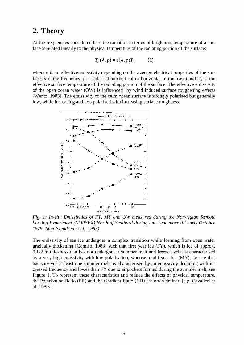
where e is an effective emissivity depending on the average electrical properties of the sur-face, λ is the frequency, p is polarisation (vertical or horizontal in this case) and TS is theeffective surface temperature of the radiating portion of the surface. The effective emissivityof the open ocean water (OW) is influenced by wind induced surface roughening effects[Wentz, 1983]. The emissivity of the calm ocean surface is strongly polarised but generallylow, while increasing and less polarised with increasing surface roughness.

Fig. 1: In-situ Emissivities of FY, MY and OW measured during the Norwegian RemoteSensing Experiment (NORSEX) North of Svalbard during late September till early October1979. After Svendsen et al., 1983)

The emissivity of sea ice undergoes a complex transition while forming from open watergradually thickening [Comiso, 1983] such that first year ice (FY), which is ice of approx.0.1-2 m thickness that has not undergone a summer melt and freeze cycle, is characterisedby a very high emissivity with low polarisation, whereas multi year ice (MY), i.e. ice thathas survived at least one summer melt, is characterised by an emissivity declining with in-creased frequency and lower than FY due to airpockets formed during the summer melt, seeFigure 1. To represent these characteristics and reduce the effects of physical temperature,the Polarisation Ratio (PR) and the Gradient Ratio (GR) are often defined [e.g. Cavalieri etal., 1993]:

6

PRT V T H

T V T H

GRT p T p

T p T p

B B

B B

pB B

B B

λ

λ λ

λ λλ λ

λ λλ λ

=−+

=−+

( , ) ( , )

( , ) ( , )

( , ) ( , )

( , ) ( , )1 2

2 1

2 1

(2)

with the same notation as earlier. PR19 is practically insensitive to ice type variations, it issmall over ice and large over open water. GR1937V reflects the sensitivity to frequency of MYice and OW such that GR1937V < 0 for MY ice and GR1937V > 0 for OW and GR1937V ≈ 0 forFY ice. In addition to these surface types numerous other ice types, e.g. new ice, may befound having different radiational properties. However, with the set of channels and resolu-tion featured on presently operating satellite systems it is not feasible to distinguish themfrom a mixture of MY, FY and OW [Wensnahan et al., 1993]. The emissivity of the con-solidated ice sheet additionally varies considerably during the meltseason due to wetness ofthe snowcover and due to the formation of meltponds. The former effect brings about a par-ticularly large increase in the emissivity of the MY ice attaining values very close to that ofFY.

The radiation received by the SSM/I sensor consists of contributions from the surface asgiven by equation 1 minus the atmospheric attenuation as well as contributions from theatmosphere and from space. This can be described by a radiative transfer equation:

T p e p T e T

e p T e e p T e

B S B up

B down B sp

( , ) ( , ) ( )

[ ( , )] ( ) [ ( , )] ( )

( ),

,( )

,( )

λ λ λ

λ λ λ λ

τ λ

τ λ τ λ

= + +

− + −

−

− −1 1 2(3)

where TB,up and TB,down denote upwelling and downwelling atmospheric radiation, TB,sp isthe radiation from space and τ is the atmospheric opacity. For the rain free atmosphere, theRayleigh criterion is applicable, i.e. scattering effects are negligible, up to 50 GHz (Ulaby etal., 1981). Furthermore, under Arctic conditions, the water content of the atmosphere issmall and the attenuation is therefore small. Under rainy conditions or at frequencies above50 GHz, however, scattering effects are important and give rise to increased atmosphericabsorption as well as emission.

In the retrieval of ice parameters from satellite passive microwave radiometry, the atmos-pheric contributions are relatively small over the bright FY ice surfaces and most notablyresult in spurious ice concentrations over the open ocean as well as deficient MY concentra-tions. As a response to problems with spurious ice, simple thresholding filters to reject spu-rious pixels have been applied [Gloersen & Cavalieri, 1986; Cavalieri et al., 1995]. A morephysically based approach is to retrieve atmospheric parameters (surface wind, liquid waterpath and integrated water vapour) from the SSM/I brightness temperatures over water andcorrect for them [Heygster et al., 1996]. Within the present project the use of NumericalWeather Prediction (NWP) model fields for a similar correction scheme will be described ina coming report.

Previous studies on tiepoints [e.g. Pedersen, 1991; Thomas, 1993] have often concentratedon enhancing specific aspects like bias or interannual consistency in ice concentration retri-vals. Others [e.g. Svendsen et al., 1983] have based their tiepoints on field measurements ofemissivity (see Figure 1), which is physically superior. However, monthly data to accountfor the full annual cycle are not available and it is difficult to assure representativity of thein-situ samples. Furthermore, the use of the atmospheric correction scheme mentioned

7

above and the more rigorous accounting for terms 1, 2 and 3 of equation 3, supports a dif-ferent emphasis in the definition of tie-points. Thus, in the following tiepoints are taken tobe typical emissivities characterising the individual surface type including the effect of amean climatological (well-known) atmospheric state. In summary the objective is thereforeto establish a data set that reflects the average monthly variation in surface emissivity plusatmospheric contributions. Hence, the possibility in a subsequent algorithm definition toaccount for surface temperature variations and atmospheric influences explicitly by meansof auxiliary data is kept open.

8

3. Data and Methodology

3.1 Data

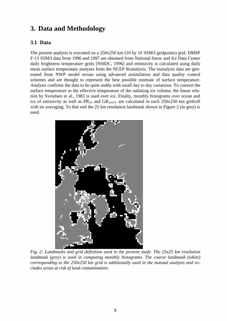
The present analysis is executed on a 250x250 km (10 by 10 SSM/I gridpoints) grid. DMSPF-13 SSM/I data from 1996 and 1997 are obtained from National Snow and Ice Data Centerdaily brightness temperature grids [NSIDC, 1996] and emissivity is calculated using dailymean surface temperature analyses from the NCEP Reanalysis. The reanalysis data are gen-erated from NWP model reruns using advanced assimilation and data quality controlschemes and are thought to represent the best possible estimate of surface temperature.Analysis confirms the data to be quite stable with small day to day variations. To convert thesurface temperature to the effective temperature of the radiating ice volume, the linear rela-tion by Svendsen et al., 1983 is used over ice. Finally, monthly histograms over ocean andice of emissivity as well as PR19 and GR1937V are calculated in each 250x250 km gridcellwith no averaging. To that end the 25 km resolution landmask shown in Figure 2 (in grey) isused.

Fig. 2: Landmasks and grid definition used in the present study. The 25x25 km resolutionlandmask (grey) is used in computing monthly histograms. The coarse landmask (white)corresponding to the 250x250 km grid is additionally used in the manual analysis and ex-cludes areas at risk of land contamination.

9

3.2 Method

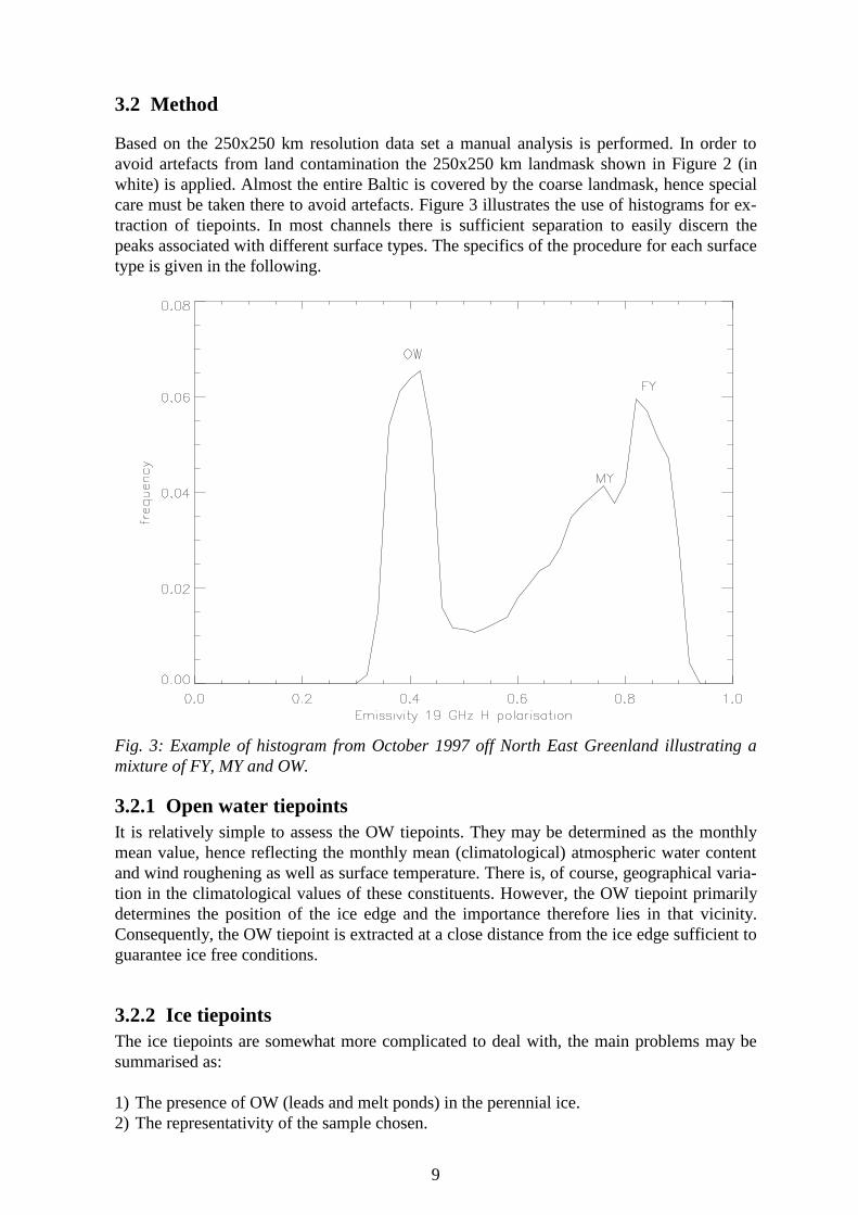
Based on the 250x250 km resolution data set a manual analysis is performed. In order toavoid artefacts from land contamination the 250x250 km landmask shown in Figure 2 (inwhite) is applied. Almost the entire Baltic is covered by the coarse landmask, hence specialcare must be taken there to avoid artefacts. Figure 3 illustrates the use of histograms for ex-traction of tiepoints. In most channels there is sufficient separation to easily discern thepeaks associated with different surface types. The specifics of the procedure for each surfacetype is given in the following.

Fig. 3: Example of histogram from October 1997 off North East Greenland illustrating amixture of FY, MY and OW.

3.2.1 Open water tiepointsIt is relatively simple to assess the OW tiepoints. They may be determined as the monthlymean value, hence reflecting the monthly mean (climatological) atmospheric water contentand wind roughening as well as surface temperature. There is, of course, geographical varia-tion in the climatological values of these constituents. However, the OW tiepoint primarilydetermines the position of the ice edge and the importance therefore lies in that vicinity.Consequently, the OW tiepoint is extracted at a close distance from the ice edge sufficient toguarantee ice free conditions.

3.2.2 Ice tiepointsThe ice tiepoints are somewhat more complicated to deal with, the main problems may besummarised as:

1) The presence of OW (leads and melt ponds) in the perennial ice.2) The representativity of the sample chosen.

10

3) Purity of the sample ice type.

For FY, it is important to choose an area of ice that is known to be of 100 % concentrationand located in the seasonal ice zone to avoid contamination with MY ice. To aid in locatingsuch areas, a-priori knowledge along with images of PR19 are used in choosing gridcellscharacterised by minimum PR19 and the highest emissivity characterised by a peak in thehistogram is selected as the tiepoint. During winter this is straightforward and the validity ofthe tiepoint rests on the assumption that the statistics of the 250x250 km grid cell are domi-nated by pixels of 100% ice concentration. This procedure is similar to the one adopted byThomas, 1993.

During summer the ice is broken up and the surface is extensively covered by melt ponds. Inaddition the MY ice looses its characteristics and merges with the FY ice into a summer icesignature, rendering ice type analyses impossible [e.g. Comiso, 1983]. The ice emissivityduring summer is very variable; it is determined by the extent of melt ponds that lead to de-creased emissivity and wet snow cover effects that lead to increased emissivities. In additioncome uncertainties in the extent of cracks and leads, however, previous studies show that iceconcentrations during summer are very high, between 90 and 100% [Carsey, 1982; Camp-bell et al., 1984; Barry and Maslanik, 1989]. Melt ponds may affect up to 80 % of the sea icesurface [Grenfell and Lohanick, 1985] and is a fundamental problem that cannot be distin-guished from leads or cracks. It will lead to seriously depressed ice concentrations if onechooses the overall maximum emissivity (that corresponds to wet snow) as tiepoint duringsummer. In order to reduce these effects we choose gridcells characterised by high PR19 tolocate areas with a low extent of open water (i.e. cracks, leads and meltponding) and themean emissivity within these cells to avoid the wet snow signature. This will of course leadto larger occurrences of total ice concentration estimates in excess of 100% during summerbut the mean hemispheric concentration should remain closer to the true value.

By definition, the ice cover that is present by the fall freezeup is classified as MY. However,the MY tiepoint is even more problematic than the FY as old leads freeze up and yield anunknown mixture of OW, MY and FY. Furthermore there is evidence that the radiativeproperties of the MY ice itself is varying considerably over time, which gives rise to a lackof consistency in the retrieved MY ice coverage. The procedure for establishing the MYtiepoint is to use GR1937V to enable the identification of gridcells of high MY concentration[Cavalieri and Gloersen, 1984]. Subsequently, the assessment of the tiepoint is based on useof histograms in conjunction with experience from previously published works [e.g. Svend-sen et al., 1983; Comiso, 1983; Pedersen, 1991; Eppler et al., 1992; Steffen and Schweiger,1991; Thomas, 1993]. For frequencies lower than 37 GHz and all V-polarised channels, apeak in the histogram located between the peaks associated with OW and FY representsMY. For H-polarised frequencies from 37 GHz and up, the emissivity of MY is less thanthat of OW, which simplifies the tiepoint extraction to that of the generally lowest emissiv-ity peak within the MY ice pack.

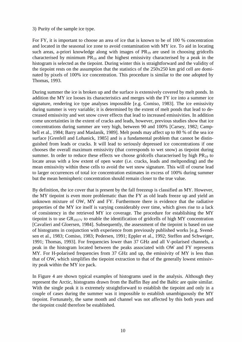
In Figure 4 are shown typical examples of histograms used in the analysis. Although theyrepresent the Arctic, histograms drawn from the Baffin Bay and the Baltic are quite similar.With the single peak it is extremely straightforward to establish the tiepoint and only in acouple of cases during the summer was it impossible to establish unambiguously the MYtiepoint. Fortunately, the same month and channel was not affected by this both years andthe tiepoint could therefore be established.

11

Fig. 4: Typical examples of histograms used to define tiepoints from October 1997. The leftrepresents FY ice in the Kara Sea, the right panel represents MY ice off the Canadian Ar-chipelago. Notice that in both cases the histogram contains only one peak, facilitating thedetermination of the tiepoints. Although this sample is drawn from the Arctic Ocean, similarhistograms are obtained in the Baltic and in the Baffin Bay.

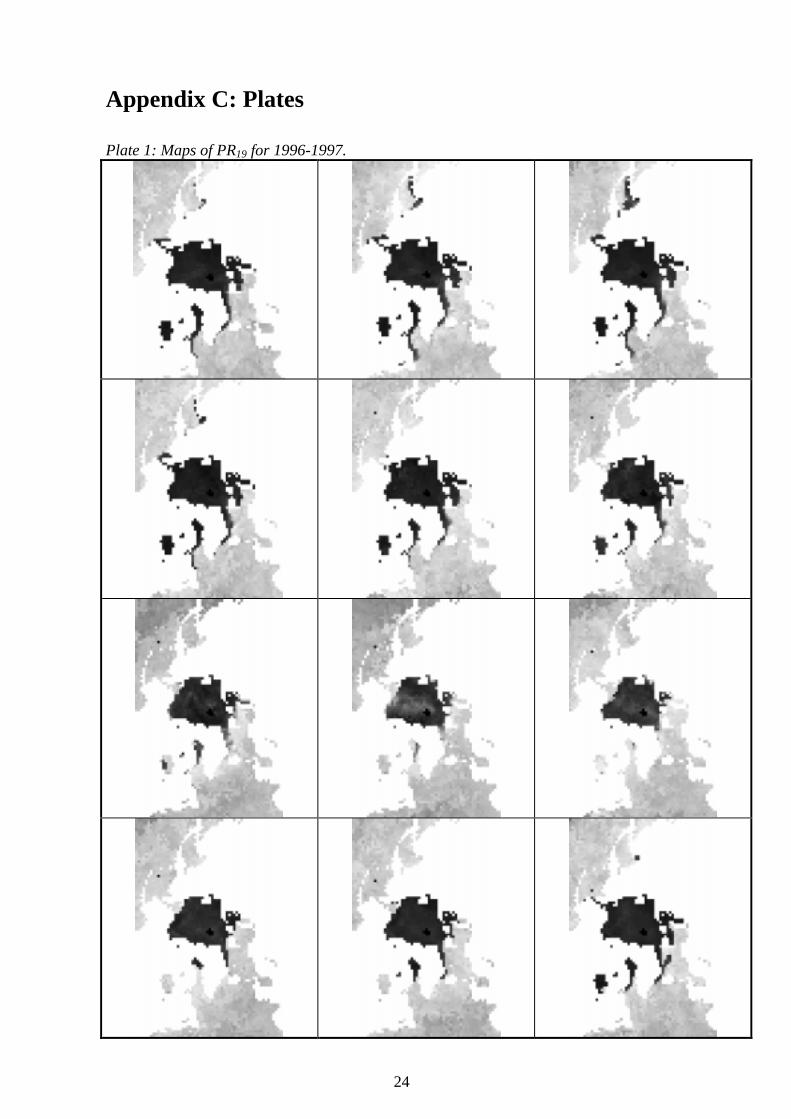
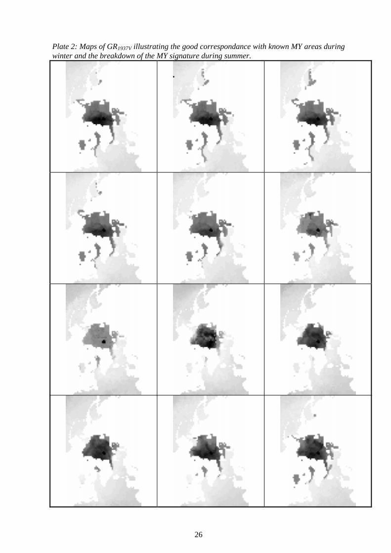
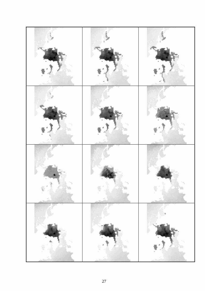
As can be seen from plates 1 and 2 (found in Appendix C), the Arctic ice season of 1996was characterised by less extensive breakup than usual leaving large expanses of the Kara,Barents and Laptev Seas ice covered although they are usually ice free during summer. Atthe same time the East Coast of Greenland experienced very mild ice conditions. Accord-ingly, at the onset of freezing conditions in autumn of 1996 until the melt season of 1997,areas characterised by ice of large negative GR1937V (MY signature) are found in a muchwider area than usual. The summer of 1997 was much more typical as the Barents and KaraSeas this year were completely free of ice during the summer. At the onset of freezing theice characterised by low GR1937V is seen to retreat considerably towards the Canadian Ar-chipelago. As a consequence of these conditions great care must be exercised when estab-lishing the FY tiepoint after the summer of 1996 in order to avoid areas of 2’nd year ice. It isfound, however, that areas of the Laptev, Kara and Barents Seas are characterised byGR1937V close to zero, minimum PR19 as well as overall maximum emissivities which can betaken as strong evidence that there are in fact pixels within this area covered completely byFY ice. Consequently the Arctic FY tiepoint is taken from this general area.

In the Baffin Bay the ice usually melts completely during summer. However, in 1996 thiswas not the case and consequently MY ice might be found in a small area close to theGreenland Coast during the winter of 1996/1997. This leads to avoidance of the area closestto the Greenland Coast when establishing the FY tiepoint as it is most likely to contaminatethe tiepoint with MY ice. Although the ice did not vanish completely, the widespread meltduring July-September was found to destroy the possibility of establishing a credible tie-point.

In the Baltic the ice melts completely during summer, hence it is not necessary to considercontamination of the FY signature with old ice. Rather it is the possible contamination byland that requires careful analysis to avoid introduction of artefacts. The ice extent is gener-ally only sufficient to allow determination of tiepoints during the months from Januarythrough April.

12

4. Results

Following the methodology given in the previous section the set of tiepoints for the ArcticOcean, the Baffin Bay and the Baltic were determined. The results are given in Tables 1-3for the Arctic Ocean, Tables 4-5 for the Baffin Bay and Tables 6-7 for the Baltic. The Tablesare found in Appendix A, while plots of the tiepoints can be found in Appendix B. Not sur-prisingly the difference in the tiepoint emissivity estimates between years was highest in thesummer months attaining values as high as 0.06 for the 85H MY tiepoint during August. Forthe lower frequencies and for FY and OW tiepoints in general there was much better con-sistency from year to year. The maximum difference was 0.04, again in the month ofAugust. Over all, a typical difference in emissivity was found to be about 0.01.

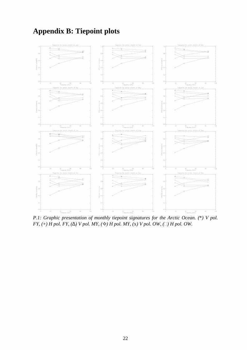
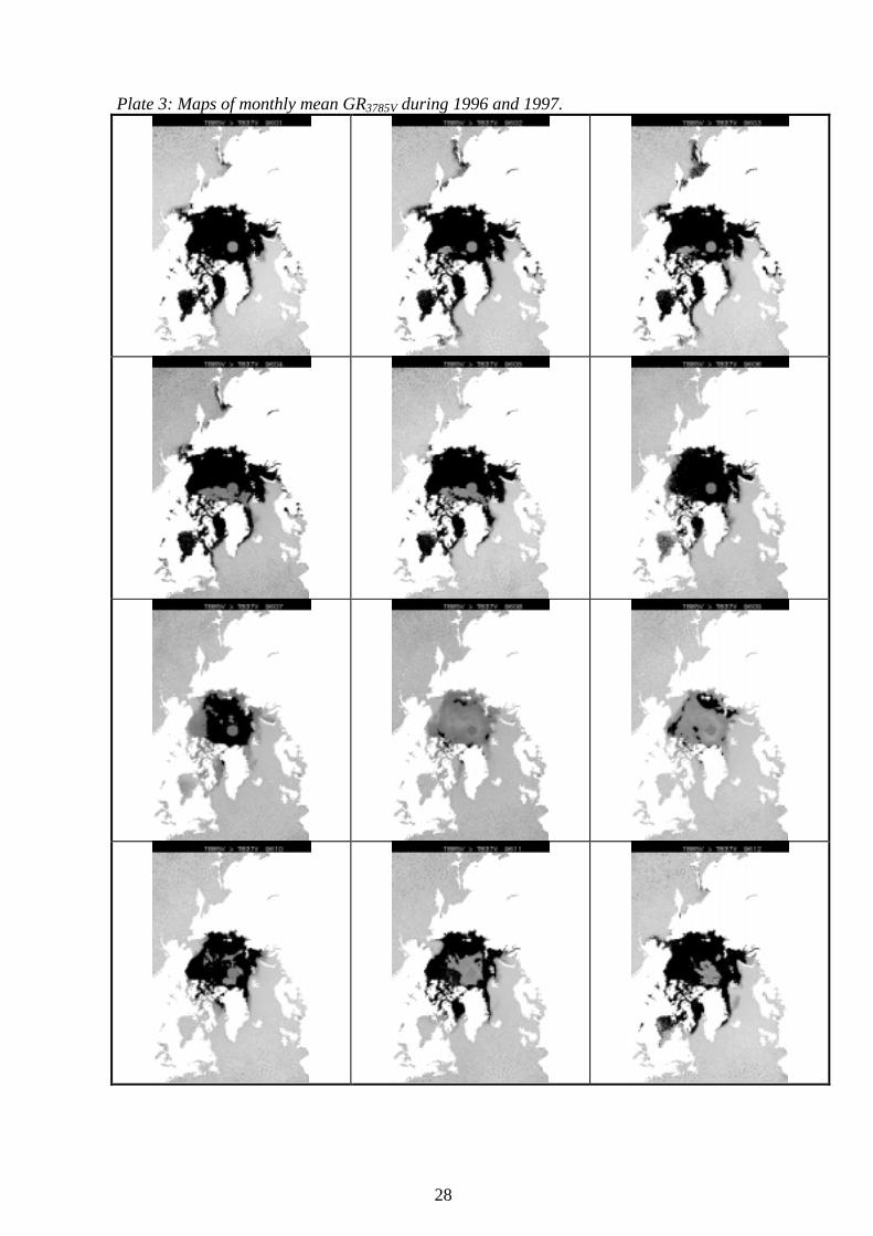
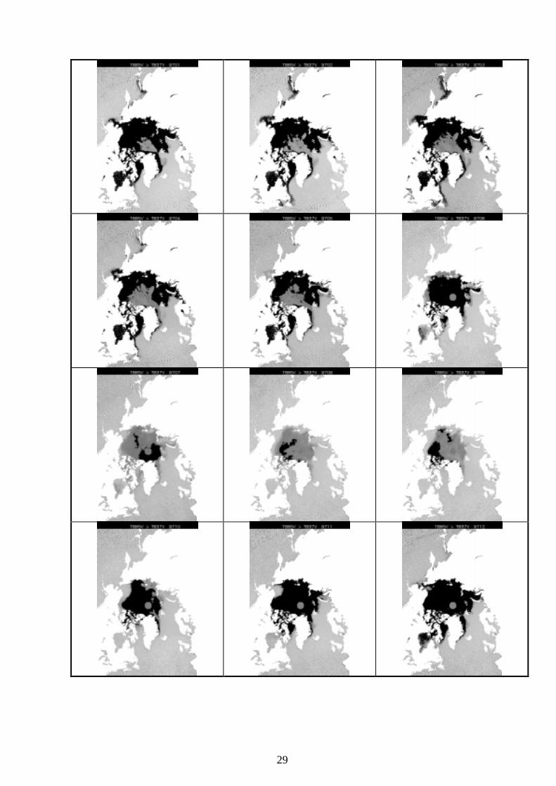
In the Arctic based on PR19 and GR1937V all MY tiepoints were found in a well confinedregion North of the Canadian Archipelago. Similarly, the FY tiepoints were found in theKara and Laptev Sea area, which is consistent with general knowledge of the Arctic ice cli-mate. Figure P.1 found in Appendix B depicts the yearly variation of these tiepoint signa-tures. Note that the polarisation ratio for ice is relatively constant throughout the year for allchannels and always in great contrast to the polarisation ratio for OW. During the wintermonths the tiepoints are generally in reasonable accordance with the emissivities measuredduring NORSEX (see Figure 1). One exception is the evolution of the MY tiepoint at 85GHz that for several months is even higher than that for 37 GHz. This is in contrast to theNORSEX measurements and surprising as one would expect the increased scattering in MYto attenuate the emissivity of the 85 GHz channel. To investigate the nature of the phenome-non more closely images of monthly mean GR3785V for 1996 and 1997 where negative val-ues (corresponding to agreement with the NORSEX signatures) are masked out are pre-sented in plate 3, see Appendix C. Hence, under normal circumstances one would expect theentire Arctic and MY areas in particular to be masked out during winter. However, the fea-ture is seen to arise and spread from approximately February in what is known as areas ofvery old ice off the Canadian Archipelago. It vanishes abruptly in June to emerge again cov-ering almost the entire Arctic from July through October. During the months of Octoberthrough December 1997 the feature vanishes. However, during the same period of 1996 itremains and even affects the months of January through May of 1997. The origin of thephenomenon is not known to the author but may be connected with varying snow propertieslike e.g. ice crusts within the snow or salt contamination of the surface. It affects areas ofMY and FY ice indiscriminately during summer/autumn, when the effect can probably beascribed to the presence of liquid water on top of the ice. Thus, the signature is undoubtedlynot associated with the same physical property in summer and winter.

On a more general level, at the onset of summer, it is evident that the tiepoint signatures areheavily affected by surface effects arising due to melt ponds and wetness of the snow coverand the polarisation ratio over ice is increased accordingly. Especially for July, the tiepointsreflect the total merging of the MY and FY signatures. The validity of the September FYtiepoints may be argued as the minimum ice extent is generally found to occur during thatmonth [e.g. Comiso, 1990]. Accordingly, indications of OW contamination of the Septem-ber FY tiepoint are evident in the generally increased polarisation ratio.

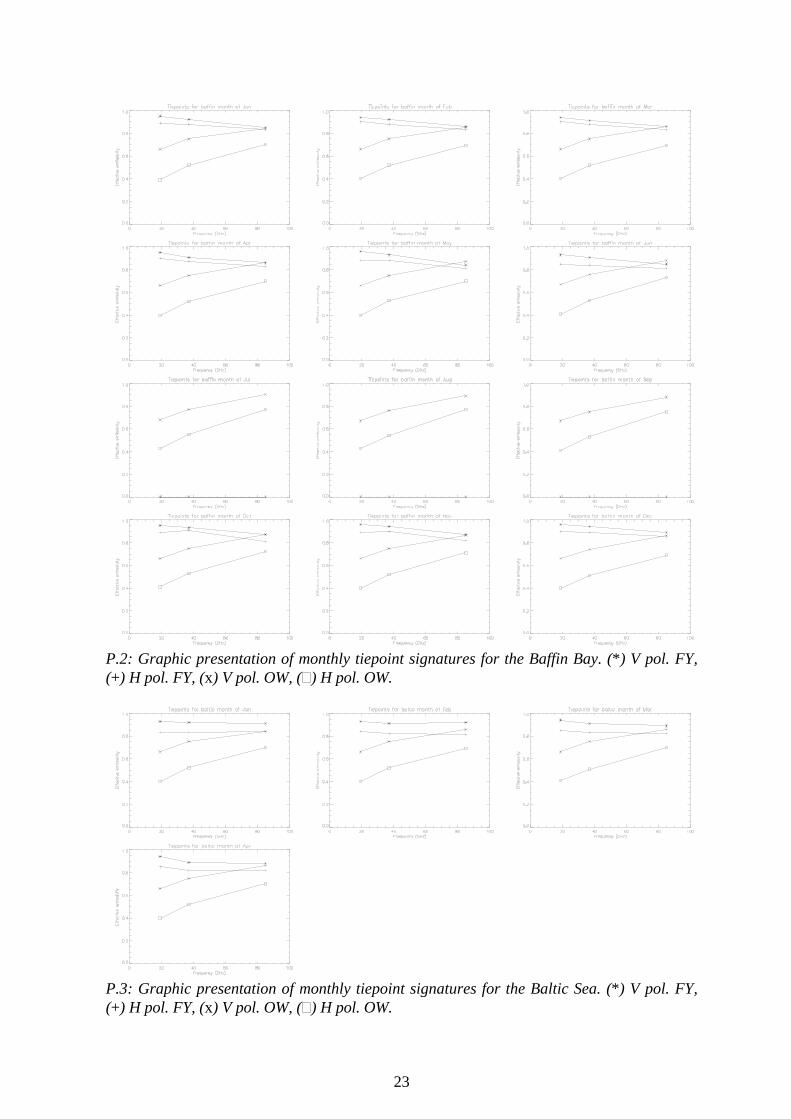
The Baffin Bay 19 and 37 GHz tiepoint emissivities (see Appendix B, Figure P.2) differonly slightly from those observed in the Arctic. The most notable distinction is probably thatthe minimum in PR37 found in both areas during October persists well into November in theBaffin Bay. At 85 GHz on the other hand large differences in the emissivity level are found

13

although PR85 is found to be relatively invariant. The polarisation ratio over ice in the Baltic(see Appendix B, Figure P.3) as compared to the two other areas is generally larger due to arelative depression in the level of the 19H and 37H channels and an increase in the 85Vlevel. There are no apparent signs of land contamination.

As for OW, the horisontally polarised signatures are most sensitive to differences in themonthly wind and water vapour distributions between different locations. The overall emis-sivity differences between the Baltic, the North Atlantic and the Baffin Bay are marginal,which is in agreement with previous works [Pedersen, 1991; Ulaby et al., 1986].

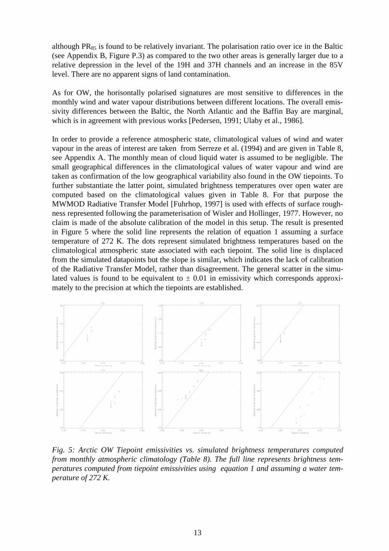
In order to provide a reference atmospheric state, climatological values of wind and watervapour in the areas of interest are taken from Serreze et al. (1994) and are given in Table 8,see Appendix A. The monthly mean of cloud liquid water is assumed to be negligible. Thesmall geographical differences in the climatological values of water vapour and wind aretaken as confirmation of the low geographical variability also found in the OW tiepoints. Tofurther substantiate the latter point, simulated brightness temperatures over open water arecomputed based on the climatological values given in Table 8. For that purpose theMWMOD Radiative Transfer Model [Fuhrhop, 1997] is used with effects of surface rough-ness represented following the parameterisation of Wisler and Hollinger, 1977. However, noclaim is made of the absolute calibration of the model in this setup. The result is presentedin Figure 5 where the solid line represents the relation of equation 1 assuming a surfacetemperature of 272 K. The dots represent simulated brightness temperatures based on theclimatological atmospheric state associated with each tiepoint. The solid line is displacedfrom the simulated datapoints but the slope is similar, which indicates the lack of calibrationof the Radiative Transfer Model, rather than disagreement. The general scatter in the simu-lated values is found to be equivalent to � 0.01 in emissivity which corresponds approxi-mately to the precision at which the tiepoints are established.

Fig. 5: Arctic OW Tiepoint emissivities vs. simulated brightness temperatures computedfrom monthly atmospheric climatology (Table 8). The full line represents brightness tem-peratures computed from tiepoint emissivities using equation 1 and assuming a water tem-perature of 272 K.

14

5. Discussion and conclusion

The tiepoints extracted here from the record of DMSP F-13 SSM/I measurements from 1996and 1997 are generally quite close to those reported in earlier works based on field meas-urements or SMMR data [Pedersen, 1991; Comiso, 1983; Svendsen, 1983] for the 19 and 37GHz channels. The 85 GHz channels, on the other hand, reveal marked differences from theNORSEX field measurements in all seasons. The unstable nature of the 85 GHz MY sig-nature certainly complicates the use of these channels for MY ice retrieval.

The differences between summer- and winter months is relatively large for both MY and FYice types although the largest variation is detected over MY. This has several reasons, suchas a larger extent of meltponding over MY ice [Grenfell and Lohanick, 1985] and the factthat the occurrence of wet snow raises the emissivity of the MY type to be comparable tothat of FY, while leaving the FY emissivity relatively unaffected. The breakdown of theseparation between MY and FY ice comes both in 1996 and 1997 in July, while the emis-sivities for June are only slightly influenced. Note that for the month of July, where theemissivities of MY at 19 and 37 GHz increase abruptly the 85 GHz emissivities are practi-cally unaffected. Except for July it is clearly possible to distinguish between two major icetypes. The critical question in summer is whether or not it is true that substantial areas of100% ice concentration with or without melt ponds exist. This is not clear at present but if itis true one should use the summer tiepoints. Otherwise an interpolation between June andOctober, thus ignoring wet snow and meltponds, might be more appropriate. Certainly, atthe time of the minimum ice extent in September, FY ice is by definition practically non-existent. The signature is accordingly smaller and more polarised indicating serious OWcontamination. It is therefore recommended to at least replace the FY signature for Septem-ber with an average of the August and October signatures. The advent and ending of thesummer melt may be readily diagnosed using the methodology outlined by e.g. Smith (1998)to determine when to start using the high emissivity July tiepoint and when to revert to alower one. It is unavoidable, however, that the summer concentration estimates will be muchmore uncertain than those of the cold seasons but the planned validation study may testsome of the above aspects and assumptions.

The geographical differences are marginal between the Arctic and the Baffin Bay. As couldbe expected, however, the difference between the Arctic and the Baltic is larger and the Bal-tic FY emissivities are generally lower, which is in accordance with the lower salinity ob-served there. At 85 GHz, on the other hand, the V-polarised emissivity is higher while theH-polarised one is at approximately the same level as observed elsewhere.

The present study bears some implications for algorithm development. Plate 3 (see Appen-dix C) presents large interannual variations in the signature of MY at 85 GHz. This is clearevidence that it is presently not feasible to use the 85 GHz channel for ice type classifica-tions. However, once the reasons for the observed behaviour is understood it might add in-teresting knowledge on other important aspects. It is observed that the polarisation ratio re-mains at a relatively constant level throughout the year and that the differences between MYand FY ice are small. This confirms the usefulness of the parameter for total ice concentra-tion retrieval at 85 GHz as it is found by Svendsen et al. (1987). The much increased sensi-tivity to atmospheric noise, however, is still an unresolved issue [Lubin et al., 1997].

It is anticipated that the tiepoints presented here will be able to contribute to more exact re-trievals of both FY and especially MY when used in conventional algorithms based on the

15

19 and 37 GHz channels. Furthermore it facilitates a more consistent accounting for the ef-fects of the atmosphere as it allows the definition of a reference atmospheric state from cli-matology associated with each individual tiepoint. This is feasible due to the fact that inpractice the tiepoints for each individual surface type are retrieved in a relatively well con-fined area from month to month. For completeness, total precipitable water, wind speed re-duced to 10 m and surface pressure, extracted at representative locations from climatology[Serreze et al., 1994] are given in Table 8 and their consistency with the OW tiepoints isillustrated in Figure 5.

5.1 Recommendations

The present set of tiepoint have been determined to accommodate the use of auxiliary datafor elimination of e.g. atmospheric effects and effects of surface temperature. For mostmonths it is recommended that the tiepoints be interpolated linearly in time to avoid discon-tinuities in the retrieved concentrations at the turn of each month. The FY tiepoints for Sep-tember do not seem valid and should therefore be replaced by an interpolation of the adja-cent months. In the remaining summer months the ice tiepoint estimation may also sufferfrom water contamination in the form of cracks and leads. The extent is unknown and indis-tinguishable from melt ponds. However, as reference data on actual ice concentrations (withor without melt ponds) is needed, it is left to a planned ice algorithm validation study to as-sess the validity and usefulness of the remaining summer tiepoints. To assure and assess thevalidity of long term retrievals made with any kind of tiepoint set, the interannual variationsin tiepoint emissivity should be assessed using a much longer dataset than the one used here.

16

6. Acknowledgements

The present report describes the outcome of work performed during the authors stay as avisiting scientist under the EUMETSAT SAF on Ocean and Sea Ice development project atthe National/Naval Ice Center, Washington D.C. For assistance and fruitful discussion dur-ing the stay thanks are extended to Kim Partington and Adnan Trakic, NIC as well as RobertGrumbine, NCEP and Don Cavalieri, NASA GSFC. Leif Toudal Pedersen is thanked forproviding valuable comments to the manuscript. NCEP Reanalysis data provided by theNOAA-CIRES Climate Diagnostics Center, Boulder, Colorado, from their Web site athttp://www.cdc.noaa.gov/ is used in this work.

17

7. References

Barry, R.; J. Maslanik: Arctic sea ice characteristics and associated atmosphere - ice inter-actions in summer inferred from SMMR data and drifting buoys: 1979-1984, Geojournal,18, 1, 1989.

Campbell, W. J.; P. Gloersen; H. J. Zwally: Aspects of Arctic sea ice observable by sequen-tial passive microwave observations from the Nimbus-5 satellite, in I. Dyer and C. Chrys-sotomidis (Ed.): Arctic Technology and Policy, 197-122, Hemisphere, New York, 1984.

Cavalieri, D. J.; K. M. St. Germain; C. T. Swift: Reduction of weather effects in the calcu-lation of sea-ice concentration with the DMSP SSM/I, J. Glaciol., 41, 139, 455-464, 1995.

Cavalieri, D. J.; P. Gloersen: Determination of sea ice parameters with the Nimbus 7SMMR, J. Geophys. Res., 89, C4 , 5355-5369, 1984.

Comiso J.C.: Characteristics of Arctic winter sea ice from satellite multispectral microwaveobservations, J. Geophys. Res., 91, C1, 975-994, 1986.

Comiso, J. C.: Arctic multiyear ice classification and summer ice cover using passive mi-crowave satellite data, J. Geophys. Res., 95, C8 , 13411-13422, 1990.

Comiso, J. C.: Sea ice effective microwave emissivities from satellite passive microwaveand infrared observations, J. Geophys. Res., 88, C12, 7686-7704, 1983.

Eppler, D.; M. R. Anderson; D. J. Cavalieri; J. C. Comiso; P. Gloersen; C. Garrity; T. C.Grenfell; M. Hallikainen; J. A. Maslanik; C. Mätzler; R. A. Melloh; I. Rubinstein; C. Swift:Passive microwave signatures of sea ice. In Carsey (Ed.): Microwave remote sensing of seaice, American Geophysical Union, Washington DC, 48-71, 1992.

Fuhrhop, R.: MWMOD user manual, Institut für Meereskunde, Christian-Albrechts-Universität, Kiel, Germany, 82 pp., 1997.

Gloersen, P.; D. J. Cavalieri: Reduction of weather effects in the calculation of sea ice con-centration from microwave radiances, J. Geophys. Res., 91,C3 , 3913-3919, 1986.

Grenfell, T. C.; A. W. Lohanick: Temporal variations of the microwave signatures of sea iceduring the late spring and early summer near Mould Bay NWT, J. Geophys. Res., 90, C3 ,5063-5074, 1985.

Heyster, G.; B. Burns; T. Hunewinkel; K. Künzi; L. Meyer-Lerbs; H. Schottmüller; C.Thomas; P. Lemke; T. Viehoff; J. Turner; S. Harangozo; T. Lachlan-Cope; L. T. Pedersen:Pelicon - Project for estimation of long term variability in ice concentration, Final report, ECContract EV5V-CT93-0268 (DG 12 DTEE), 188 pp., 1996.

Lubin, D.; C. Garrity; R. O. Ramseier; R. H. Whritner: Total sea ice concentration retrievalfrom the SSM/I 85.5 GHz channels during the arctic summer. Remote Sens. Environ., 62,63-76, 1997.

18

Oelke C.: Atmospheric signatures in sea-ice concentration estimates from passive micro-waves: modelled and observed, Int. J. Remote Sensing, 18, 5, 1113-1136, 1997.

Parkinson C. L., J. C. Comiso, H. J. Zwally, D. J. Cavalieri, P. Gloersen, W. J. Campbell:Arctic sea ice, 1973-1976: Satellite passive microwave observations, NASA-SP-489, 296pp., 1987.

Pedersen, L. T.: Retrieval of sea ice concentration by means of passive microwave radiome-try, PhD dissertation LD 81, Electromagnetics Institute, Technical University of Denmark,148 pp., 1991.

Rothrock D. A., D. R. Thomas, A. S. Thorndike: Principal component analysis of satellitepassive microwave data over sea ice, J. Geophys. Res., 93, C3, 2321-2332, 1988.

Serreze M. C., M. C. Rehder, R. G. Barry, and J. D. Kahl: A climatological data base ofArctic water vapor characteristics. Polar Geography and Geology, 18, 63-75, 1994.

Smith D. M.: Recent increase in the length of the melt season of perennial Arctic sea ice,Geophysical Research Letters, 25, 5, 655-658, 1998

Steffen K.; A. Schweiger: NASA Team algorithm for sea ice concentration retrieval fromDefense Meteorological Satellite Program Special Sensor Microwave Imager: Comparisonwith Landsat imagery. J. Geophys. Res., 96, C12, 21971-21987, 1991.

Svendsen E.; K. Kloster; B. Farelly; O. M. Johannesen; J. A. Johannesen; W. J. Campbell;P. Gloersen; D. J. Cavalieri; C. Mätzler: Norwegian remote sensing experiment: Evaluationof the Nimbus 7 scanning multichannel microwave radiometer for sea ice research. J. Geo-phys. Res., 88, C5, 2781-2791, 1983.

Svendsen E.; C. Mätzler; T. C. Grenfell: A model for retrieving total sea ice concentrationfrom spaceborne dual-polarised passive microwave instrument operating near 90 GHz. Int.J. Remote Sensing, 8, 10, 1479-1487, 1987.

Thomas D. R.: Arctic sea ice signatures for passive microwave algorithms, J. Geophys.Res., 98, C6, 10037-10052, 1993.

Ulaby F. T., R. K. Moore, A. K. Fung: Microwave remote sensing active and passive, vol.III: From theory to application, Artech House, Norwood, MA, 1986.

Wensnahan M., G. A. Maykut, T. C. Grenfell, D. P. Winebrenner: Passive microwave re-mote sensing of thin sea ice using principal component analysis, J. Geophys. Res., 98, C7,12453-12468, 1993.

Wentz, F.J.: Model function for ocean microwave brightness temperatures, J. Geophys.Res., 88, C3, 1892-1908, 1983.

Wilheit T. T., J. Blinn, W. Campbell, A. Edgerton, W. Nordberg: Aircraft measurements ofmicrowave emissions from Arctic sea ice, Remote Sens. Eviron., 2, 129, 1972.

19

Wisler M. M., J. P. Hollinger: Estimation of marine environmental parameters using passivemicrowave radiometric remote sensing systems, Technical Report NRL Memo Rep. 3661,Naval Research Laboratory, Washington D.C., 1977.

Zwally H. J., J. C. Comiso, C. L. Parkinson, W. J. Campbell, F. D. Carsey: Antarctic sea ice,1973-1976: Satellite passive-microwave observations, NASA-SP-459, 216 pp., 1983.

20

Appendix A: Tables

FY Jan Feb Mar Apr May Jun Jul Aug Sep Oct Nov Dec19V 0,95 0,94 0,95 0,95 0,96 0,96 0,93 0,90 0,88 0,95 0,96 0,9419H 0,89 0,89 0,90 0,89 0,89 0,91 0,87 0,87 0,84 0,87 0,91 0,8937V 0,92 0,92 0,91 0,92 0,93 0,94 0,92 0,92 0,88 0,92 0,94 0,9137H 0,89 0,88 0,88 0,88 0,88 0,89 0,86 0,85 0,78 0,88 0,89 0,8885V 0,84 0,89 0,84 0,84 0,86 0,87 0,85 0,82 0,84 0,84 0,88 0,8285H 0,82 0,84 0,83 0,82 0,84 0,83 0,83 0,77 0,74 0,76 0,83 0,78

MY Jan Feb Mar Apr May Jun Jul Aug Sep Oct Nov Dec19V 0,83 0,83 0,84 0,85 0,86 0,87 0,94 0,81 0,81 0,83 0,83 0,8419H 0,76 0,77 0,77 0,78 0,79 0,80 0,88 0,74 0,72 0,76 0,75 0,7637V 0,70 0,71 0,71 0,72 0,75 0,78 0,93 0,67 0,71 0,72 0,71 0,7037H 0,65 0,66 0,66 0,67 0,69 0,72 0,88 0,63 0,66 0,67 0,66 0,6685V 0,67 0,69 0,72 0,75 0,77 0,80 0,77 0,74 0,74 0,73 0,75 0,7085H 0,65 0,66 0,66 0,71 0,74 0,74 0,75 0,72 0,72 0,71 0,72 0,67

OW Jan Feb Mar Apr May Jun Jul Aug Sep Oct Nov Dec19V 0,66 0,66 0,66 0,66 0,66 0,67 0,67 0,67 0,67 0,66 0,66 0,6619H 0,40 0,40 0,40 0,40 0,40 0,41 0,42 0,42 0,41 0,41 0,40 0,4037V 0,75 0,75 0,75 0,75 0,75 0,76 0,76 0,76 0,75 0,75 0,75 0,7437H 0,52 0,52 0,52 0,52 0,52 0,53 0,54 0,54 0,53 0,53 0,52 0,5285V 0,84 0,85 0,86 0,86 0,87 0,88 0,89 0,89 0,88 0,87 0,86 0,8685H 0,70 0,69 0,69 0,70 0,70 0,73 0,75 0,76 0,75 0,72 0,71 0,69Tables 1-3: Tiepoint emissivities for FY, MY and OW measured over or in the vicinity ofthe Arctic Ocean.

FY Jan Feb Mar Apr May Jun Jul Aug Sep Oct Nov Dec19V 0,95 0,94 0,94 0,95 0,96 0,93 0,95 0,96 0,9619H 0,89 0,90 0,90 0,90 0,88 0,85 0,89 0,89 0,9037V 0,92 0,92 0,91 0,91 0,93 0,91 0,93 0,94 0,9437H 0,88 0,88 0,88 0,87 0,88 0,84 0,91 0,90 0,8985V 0,85 0,86 0,86 0,86 0,84 0,85 0,87 0,87 0,8985H 0,83 0,83 0,83 0,83 0,81 0,81 0,81 0,82 0,85

OW Jan Feb Mar Apr May Jun Jul Aug Sep Oct Nov Dec19V 0,66 0,66 0,66 0,66 0,66 0,67 0,68 0,67 0,67 0,66 0,66 0,6619H 0,39 0,40 0,40 0,40 0,40 0,41 0,43 0,43 0,41 0,41 0,40 0,4037V 0,75 0,75 0,75 0,75 0,75 0,76 0,77 0,76 0,75 0,75 0,75 0,7437H 0,52 0,52 0,52 0,52 0,53 0,53 0,55 0,54 0,53 0,53 0,52 0,5185V 0,84 0,85 0,86 0,86 0,87 0,88 0,90 0,89 0,88 0,87 0,86 0,8685H 0,70 0,69 0,69 0,70 0,70 0,73 0,77 0,77 0,75 0,72 0,71 0,69Tables 4-5: Tiepoint emissivities for FY ice and OW measured over the Baffin Bay.

21

FY Jan Feb Mar Apr May Jun Jul Aug Sep Oct Nov Dec19V 0,93 0,93 0,94 0,9419H 0,83 0,84 0,85 0,8537V 0,92 0,91 0,91 0,8937H 0,83 0,82 0,83 0,8285V 0,91 0,92 0,89 0,8885H 0,84 0,81 0,82 0,82

OW Jan Feb Mar Apr May Jun Jul Aug Sep Oct Nov Dec19V 0,66 0,66 0,66 0,6619H 0,40 0,40 0,41 0,4037V 0,75 0,75 0,75 0,7537H 0,52 0,52 0,51 0,5285V 0,84 0,86 0,86 0,8685H 0,70 0,69 0,70 0,70Tables 6-7: Tiepoint emissivities for FY ice and OW measured over the Baltic Sea duringthe ice seasons of 1996 and 1997.

Arctic Jan Feb Mar Apr May Jun Jul Aug Sep Oct Nov DecFY PW 2,00 2,03 2,26 3,10 5,69 10,35 13,90 12,41 8,50 4,34 2,72 2,26

MY PW 1,79 1,59 1,78 2,46 4,80 9,16 12,33 10,91 7,11 3,45 2,17 1,90

PW 4,77 5,28 5,24 6,37 8,29 11,71 15,06 14,44 12,36 9,21 6,71 5,28

OW MW 1,00 -1,10 -0,57 -0,30 -0,20 0,17 -0,30 -0,57 0,00 -0,17 0,13 0,93

ZW -1,03 -0,53 -1,47 1,33 -1,40 -0,10 0,27 0,16 -0,40 -0,20 -1,50 -2,87

Baffin Jan Feb Mar Apr May Jun Jul Aug Sep Oct Nov DecFY PW 2,45 2,35 3,07 3,36 5,62 9,80 13,49 11,94 9,42 5,10 3,46 2,78

PW 3,07 3,04 4,15 4,89 7,44 13,28 18,59 15,83 12,31 7,01 4,78 3,67

OW MW -0,51 0,07 0,16 0,02 0,05 0,10 -0,47 0,02 0,07 0,09 -0,12 0,09

ZW 1,87 1,43 1,09 -0,25 -1,15 -1,25 -1,45 -1,06 0,55 -0,05 1,00 1,41

Table 8: Precipitable water (PW) in mm, zonal wind (ZW) and meridional wind (MW) inm/s from climatology [Serreze et al., 1994] in areas representative to the tiepoint extraction.

22

Appendix B: Tiepoint plots

P.1: Graphic presentation of monthly tiepoint signatures for the Arctic Ocean. (* ) V pol.FY, (+) H pol. FY, (∆) V pol. MY, (✧) H pol. MY, (x) V pol. OW, (�) H pol. OW.

23

P.2: Graphic presentation of monthly tiepoint signatures for the Baffin Bay. (* ) V pol. FY,(+) H pol. FY, (x) V pol. OW, (�) H pol. OW.

P.3: Graphic presentation of monthly tiepoint signatures for the Baltic Sea. (* ) V pol. FY,(+) H pol. FY, (x) V pol. OW, (�) H pol. OW.

24

Appendix C: Plates

Plate 1: Maps of PR19 for 1996-1997.

25

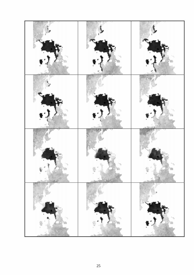
26

Plate 2: Maps of GR1937V illustrating the good correspondance with known MY areas duringwinter and the breakdown of the MY signature during summer.

27

28

Plate 3: Maps of monthly mean GR3785V during 1996 and 1997.

29