DATA DISTRIBUTION IN HPX

DATA DISTRIBUTION IN HPX

A Thesis

Submitted to the Graduate Faculty of the Louisiana State University and

Agricultural and Mechanical College in partial fulfillment of the

requirements for the degree of Master of (degree)

in

System Science

by Bibek Ghimire

B.S., Louisiana State University, 2012 December 2014

ii

ACKNOWLEDGEMENTS

I would like to thank Dr. Hartmut Kaiser from the Center for Computation and

Technology for his constant support and opportunity. He has provided tremendous support

during the pursue of my graduate study. My gratitude goes to the entire member from Ste||ar

group of Center for Computation and Technology for providing suggestions and feedbacks. I

would also like to thank my committee members Dr. Hartmut Kaiser, Dr. Steven Brandt and Dr.

Jianhua Chen for their constructive criticism. I would also like to thank Anuj R. Sharma for his

work in distributed vector. Finally I would like to thank my parents for their constant support and

motivations and thank you goes to all the people whom I have met and spent good times.

iii

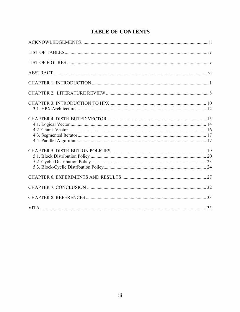
TABLE OF CONTENTS

ACKNOWLEDGEMENTS ............................................................................................................ ii

LIST OF TABLES ......................................................................................................................... iv

LIST OF FIGURES ........................................................................................................................ v

ABSTRACT ................................................................................................................................... vi

CHAPTER 1. INTRODUCTION ................................................................................................... 1

CHAPTER 2. LITERATURE REVIEW ....................................................................................... 8

CHAPTER 3. INTRODUCTION TO HPX .................................................................................. 10 3.1. HPX Architecture .............................................................................................................. 12

CHAPTER 4. DISTRIBUTED VECTOR .................................................................................... 13 4.1. Logical Vector ................................................................................................................... 14 4.2. Chunk Vector ..................................................................................................................... 16 4.3. Segmented Iterator ............................................................................................................. 17 4.4. Parallel Algorithm .............................................................................................................. 17

CHAPTER 5. DISTRIBUTION POLICIES ................................................................................. 19 5.1. Block Distribution Policy .................................................................................................. 20 5.2. Cyclic Distribution Policy ................................................................................................. 23 5.3. Block-Cyclic Distribution Policy ....................................................................................... 24

CHAPTER 6. EXPERIMENTS AND RESULTS ........................................................................ 27

CHAPTER 7. CONCLUSION ..................................................................................................... 32

CHAPTER 8. REFERENCES ...................................................................................................... 33

VITA ............................................................................................................................................. 35

iv

LIST OF TABLES

5.1 Chunk Distribution over localities for block distribution policy ……………………….….. 21

5.2 Chunk Distribution over localities for cyclic distribution policy ………………….………. 23

5.3 Chunk Distribution over localities for block-cyclic distribution policy ……………….……25

v

LIST OF FIGURES

Figure 4.1. Representation of distributed vector hpx::vector v(16,hpx::block(4)) ……………...15

Figure 5.1. Shows how the mapping of distributed vector elements are done in block distribution policy hpx::vector v(16,hpx::block(4))………………………………...22

Figure 5.2. Shows how the mapping of distributed vector elements are done in cyclic

distribution policy hpx::vector v(16,hpx::cyclic(4)) ……………………………….24 Figure 5.3: Shows how the mapping of distributed vector elements are done in

block-cyclic distribution policy hpx::vector v(16,hpx::block_cyclic(2,4)) ...………26 Figure 6.1: The image of mandelbrot computed using our distributed vector …………...……...29

Figure 6.2: The graph compares distribution policies. Block, cyclic and block-cyclic with block size of 100 is plotted and compared ……………………………………30

Figure 6.3: The graph compares block-cyclic policy with different block size …………….…...31

vi

ABSTRACT

High Performance Computation (HPC) requires a proper and efficient scheme for distribution of

the computational workload across different computational nodes. The HPX (High Performance

ParalleX) runtime system currently lacks a module that automates data distribution process so

that the programmer does not have to manually perform data distribution. Further, there is no

mechanism allowing to perform load balancing of computations. This thesis addresses that issue

by designing and developing a user friendly programming interface conforming to the C++11/14

Standards and integrated with HPX which enables to specify various distribution parameters for

a distributed vector. We present the three different distribution policies implemented so far:

block, cyclic, and block-cyclic. These policies influence the way the distributed vector maps any

global (linear) index into the vector onto a pair of values describing the number of the (possibly

remote data partition) and the corresponding local index. We present performance analysis

results from applying the different distribution policies to calculating the Mandelbrot set; an

example of an ‘embarrassingly parallel’ computation. For this benchmark we use an instance of a

distributed vector where each element holds a tuple for the current index and the value of related

to an individual pixel of the generated Mandelbrot plot. We compare the influence of different

distribution policies and their corresponding parameters on the overall execution time of the

calculation. We demonstrate that the block-cyclic distribution policy yields best results for

calculating the Mandelbrot set as it more evenly load balances the computation across the

computational nodes. The provided API and implementation gives the user a high level an

abstraction for developing applications while hiding low-level data distribution details.

1

CHAPTER 1. INTRODUCTION

High Performance Computing (HPC) has been widespread in the field of science,

engineering, art and business helping to solve complex and computationally intensive problems.

It has helped lower the execution time immensely for these computations. Without HPC it would

take days and months to do the computation, which are now solvable in few minutes or even in

seconds. Web sites like Google and Amazon use HPC to handle large volume of user since it

helps to perform large number of operations per second. From weather prediction to medical

revolution HPC has been in the forefront of scientific and computational advancements.

These complex and computationally intensive problems that we mentioned above are not

solvable using single CPU since the clock rate of a single CPU, which is the speed at which it

executes computation are not sufficient enough. It requires a large number of compute elements

(CPUs and GPUs). In HPC these compute elements work in parallel to solve the problem.

Managing the use of these compute elements and tuning them to perform optimally are the major

challenge faced by HPC community.

There has been many study and work since decades to make these compute elements

work in parallel and perform faster. The vector computers of late 1970s gave bright hope on

parallel computing. It took streams of operands from memory, executed them and then sent those

streams back to the memory, which is an example of single instruction, multiple data (SIMD)[1].

But these vector-computing machines used to be very large and costly and consumed lots of

energy. “Killer micros” appeared in 1992, which had much higher clock rate then that of super

expensive vector computer and were cheaper and powerful. Many of these microprocessors

(CPUs) were connected via bus with uniform access to main memory to give a symmetric

multiprocessor (SMP). Thus SMPs having centralized shared memory system was born. The

2

importance of SMPs grew as the individual CPU’s performance reached their physical limit. This

was first step towards building cheaper super computer for HPC. Now the computation was done

in parallel over those CPUs.

The problem with those SMPs was that they could only scale to certain number of CPUs

and was not cost efficient to add increasing number of CPUs in single machine [2]. This gave

rise to number of SMPs connected via some external network and was called distributed memory

system, which was relatively cheaper to build, and gave higher scalability. Now more

computation could be done in parallel. It was called distributed because memories were spread

across the network.

For SMPs although the computation power was increasing enormously the

programmability of these machines was jeopardized. The easiness of programming single CPU

was sacrificed. Programmers now had to take care of distributing data, their total computation,

manually over each processor so that they could run in parallel, which was tedious for them.

Programmer had to view the computation in data centric manner.

For distributed memory processors the programmability was even more cumbersome

because first programmers had to take care of distributing the data all over the available SMPs

over the network first and then again further to the CPUs of individual SMPs. In addition to that

since the memory were distributed, any attempt to access memory (data) of remote SMPs had to

be explicitly stated in the program.

MPI dominated in developing application for the distributed memory system and

OpenMp for programming individual SMPs. OpenMP and MPI are still prevalent in today’s

distributed computers. However the programmability of these languages is very tedious because

programmers need to take care of data distribution and message passing factors among the

3

compute nodes themselves. This hugely reduces the productivity and code maintainability.

Programming distributed computers using MPI can be compared to “assembly language of

parallel computing” that puts a tedious overhead on the programmer’s part. Although the run

time of computation problems were decreasing using these languages was counter productive as

programing them took years to master.

There was need for a language which would take care of the data distribution and

internal message passing automatically so that programmer would only have to focus on

algorithm design. This new language needed to develop powerful compilers, which would give

programmer abstraction of serial coding by giving abstract global namespace to their data.

Underneath the hood it would automatically distribute data into the compute nodes, execute

operation on those data in parallel and also take care of message passing. This was an example of

data parallelism, where data were distributed over the processors and similar operation was done

over those processors in parallel. This kind of language would be called data parallel language.

This was simply a higher layer of abstraction of Single Instruction Multiple Data (SIMD), where

similar instruction was operated in multiple data.

Eventually many data parallel languages mushroomed trying to mitigate the problem of

programmability for parallel programming with the feature of data distribution policies. These

languages also came with different data distribution polices which determined how the global

data were to be distributed over the processors. These languages followed block and cyclic

policies for data distribution. Kali [3] was the first language for the distributed memory

architecture, which attempted to separate data distribution from algorithm. It provided global

namespace and allowed direct access to remote parts of data. The compiler of the language

4

would take care of the data distribution and message passing for accessing remote data. It had

block and cyclic of data.

From Fortran’s family Fortran D [13], Vienna Fortran, Connection Machine Fortran and

High Performance Fortran all had similar approach of exposing global namespace, which gave

programmer a view of distributed data as a single shared address space. It also used message

passing underneath the hood for the remote data access. Different of data distribution policies

like block, cyclic and block-cyclic were provided.

X10, Chapel [14], Co-array Fortran, Titanium, Unified Parallel C are some of the

languages that have addressed the problem of programmability as well, but instead of message

passing for the remote access they use Partitioned Global Address Space (PGAS) [9] which

provide programmers with single shared address space. They also provide different distribution

policies like block, cyclic and block-cyclic.

Charm++[10] has feature of dynamic load balancing and have chare array for its data

distributing. Global Array Toolkit [11] use Aggregate remote memory copy interface

[12](ARMCI) for accessing remote data.

In this thesis we provide different data distribution policies like block, cyclic and block-

cyclic for the High Performance ParallelX (HPX). HPX is based on ParallelX execution model

designed to address the challenges for future scaling in parallel application by change in

execution policy from traditional communicating sequential process (e.g. MPI) to a new concept

involving message-driven work-queue execution in context of global address space [4]. HPX

uses Active Global Address Space (AGAS), which is an extension of PGAS. The main benefit

of AGAS is it allows moving remote object in physical space without having to change the

virtual name. HPX have actions type, which wraps a C++ global function. Wrapping a function

5

in action allows it to be transported across the compute nodes and get executed as HPX thread on

them [5]. HPX component goes one step further by wrapping classes, this way member functions

of objects can now be executed remotely. Brief description of HPX is in chapter 3.

Data distribution can be of two type static data distribution and dynamic data

distribution. In static data distribution the respective data are distributed among the processors

during the compile time, where as in dynamic data distribution the data are distributed during

runtime. Languages based on PGAS are only capable of doing static data balancing since they

impose limitation on movement of object across the distributed system, but AGAS’s feature of

moving object in physical space assist in dynamic data distribution. Although current

implementation of data distribution in HPX supports static data distribution but AGAS’s feature

of moving remote object gives promising hope for future on dynamic data distribution.

For data distribution in HPX we have created a distributed vector. Logically it is a single

vector of specific size, which has functionality similar to that of C++’s standard (std) vector. But

underneath the hood, that single big vector is partitioned into smaller chunks. User specifies the

number of chunks they want to make of the big vector during the instantiation of this distributed

vector. Those chunks of vector are then distributed over the number of localities provided by the

user. Locality in HPX is a single computer or computer node. This distributed vector provides

global namespace and allows direct access to the vector elements that reside on different locality.

Each of those individual chunks of the big vector that are distributed over the localities is made

up of std vector from C++. These individual chunks are created by instantiating HPX’s

component.

6

Since our distributed vector is a collection of smaller chunks vector, a new kind of iterator was

needed. For this Segmented Iterator [6] is used for iteration over those distributed vector.

Distribution policies for the distributed vector specify how the logical single vector is to

be distributed over the localities. Other languages as stated above have data distribution features

like block, cyclic and block-cyclic as their primary data distribution policy. We also used similar

strategy for our distribution policy. User specifies the distribution policy during the instantiation

of the distributed vector.

In block distribution the logical single vector is divided into number of chunks and those

chunks are distributed over the available localities with nearest chunks close to one another. In

cyclic distribution each of the elements of logical vector is distributed over the number of chunks

in round-robin fashion and those chunks are further distributed over the localities. In block-cyclic

distribution the block of logical vector of given size is distributed into number of chunks in

round-robin fashion and those chunks are distributed over the available localities.

We tried to make the API conforming to the C++11/14 standards and integrated it with

HPX, which enables to specify various distribution parameters for a distributed vector. It takes

user specified attributes like size, value and distribution policy as argument. In the distribution

policy the user specifies the way the in which the elements of logical vector is to be distributed.

The user specified attributes of the logical vector are used to create vector over the localities

specified by the user.

We use Mandelbrot pixel calculation as our benchmark program. Different pixel of

Mandelbrot takes different time. Some take more and some take less time to compute the pixel

depending on the number of iterations it takes to compute the pixel value. Distributing the pixels

over the compute node so that all the processor gets equal amount of work gives load balanced

7

distributed computation. Which gives all the compute nodes equal amount of work. Selecting the

distribution policy results into load balanced distributed vector. In our case choosing block-

cyclic distribution policy results into load balanced computation.

In chapter 2 we go over other attempts of doing data distribution. Then we give brief

introduction on the HPX [4] in Chapter 3. Chapter 4 does the discussion on distributed vector

and its data structures. Here we talk about segmented iterator and parallel algorithm. In Chapter

5 we discuss about the distribution policy and its API design. Then in Chapter 6 we discuss about

the experiment and results. Finally in Chapter 7 we discuss on Conclusion.

8

CHAPTER 2. LITERATURE REVIEW

HPC community has been dealing with the problem of programmability in distributed

architecture. There have been many languages that have tried to mitigate the problem of

programmability in them. Our work of automatic data distribution for programmability in HPX

has been based on decades of previous research.

Kali from 1980’s was a language that provided feature of data distribution. It had a

global name space on distributed memory. The computation would be specified using parallel

loops over those global namespace [3]. Its compiler would convert the high level code into a

system of interacting tasks, which communicate via message passing and distributing data over

the respective processors. Further they advocate that the performance degradation due to lack of

true shared memory could be inhibited by the proper data distribution.

Fortran language’s extension like Fortran D, Vienna Fortran and Connection Machine

Fortran (CM Fortran) which were predecessor of High Performance Fortran (HPF) provided

facilities of data distribution [2]. Fortran D supported block, cyclic and block-cyclic distribution

policies. Here arrays are aligned to the abstract object called template, which are then mapped to

processors according to the distribution policies provided. Vienna Fortran focused manly on

irregular and adaptive program providing distribution policies like general block and indirect

distribution along with block, cyclic and block-cyclic. Similar facilities were also in CM Fortran.

Languages that use Partitioned Global Address Space (PGAS), which offers abstract

shared address space like Unified Parallel C, X-10, Co-Array Fortran and Chapel, also provide

distribution policies in them.

Charm++ [10] is the language that provides dynamic load balancing feature in it. It uses

chare array [10] for its data distribution. Global Array Toolkit [11] also provide feature of

9

distributed array, which can be distributed in certain fashion across compute nodes. It uses

Aggregate remote memory copy interface [12](ARMCI) for accessing remote data. Although

these languages provide feature of data distribution the API design still lack the user friendliness.

Chapel is by far most prominent in the field of data distribution. It provides global-view

array, which permits programmer to concentrate on algorithm rather than on data distribution

because the distribution over the distributed memory architecture is done automatically. It is

highly influenced by HPF family of languages It introduces a notion called domain, which is

first-class object linking index set, distribution, arrays and iterators [7]. The data distribution is

specified for domain whose index set is distributed over the locale. Locales are units of uniform

memory access to which data and threads can be mapped. The computation over the domain is

expressed via parallel forall loops.

We have used similar policies for data distribution as in the fore mentioned languages.

We made vector elements to be distributed over the localities using different distribution policies

like block, cyclic and block-cyclic. Our distributed vector is logically a single vector but

conceptually is made up of smaller chunks of vectors. These vectors reside on different localities

that are provided by the user.

Iterator for the distributed vector should be different than that of the normal C++ vector.

We needed an iterator that would go through all the elements that may reside on local or remote

locality and provide functionalities like copy and assignment, dereferencing, comparing for

equality and increment similar to that of normal iterators [7]. In [7] segmented data structure is

introduced which is a vector of vector or two-dimensional vector and provides insight on

segmented iterator for it. We have used his concept for our distributed vector. The segmented

iterator is used to iterate over this distributed vector.

10

CHAPTER 3. INTRODUCTION TO HPX

As we shall be moving from petascale computing to exascale in the future, we need to

reconsider the way we parallelize our code. In the prevalent programming model communicating

sequential process (MPI) two processes on different nodes have to wait on one another to send

and receive messages. This hampers the scalability of programming as well as increases its

complexity. Thus the biggest constrain for establishing efficient parallelism exist in

communication between multiple localities. Distributed memory architecture is here to stay for

long time since the single SMPs are incapable computing current magnitude of computation.

There will be applications that will require large intra-node parallelism in future. These and other

challenges of parallel programming are addressed by HPX.

HPX community came up with an acronym SLOW that addresses the major factor on

scalability and other challenges prevalent in present day popular parallel programming language

[4].

a. Starvation: Not enough work for cpu.

b. Latencies: Delay in accessing remote resources.

c. Overhead: Amount of work spent for maintaining parallel actions and resources on

critical path, which are not required for sequential program.

d. Waiting for Contention resolution: Delay caused when many threads are waiting for

shared resources.

To address these issues of SLOW, a new kind of execution model was required which would

overcome these limitations. The design principle considered addressing SLOW to build a new

kind of execution model is addressed below.

11

Instead of avoiding latency, focus was made on hiding the overall latency because latency

cannot be totally mitigated. The possibility of switching task when some precondition was not

meet to another and then again switch back to original task after the condition was met makes the

implementation of latency hiding easier. This is possible by embracing fine-grained parallelism

instead of heavy weight thread because fine-grained parallelism take fewer cycle for the context

switch.

The parallel for-loop of OpenMP exposes implicit global barrier whereas the communication

step of MPI exposes explicit global barrier. Even a single thread in any of these two cases will do

the blocking globally sometimes, which plays a huge role in degrading scaling. It needs not to

wait for the iteration whose result are produced and is needed for next operation. HPX addresses

this problem and solves using a concept called dataflow.

In MPI the data distribution is to be carried out by the programmer, which is cumbersome.

Some new HPC languages that rely on PGAS languages like chapel, UPC, X10 etc. which offer

automatic static data distribution but to address the challenge of exascale scaling dynamic data

distribution is required if load balancing impossible during static load balancing. This in HPX is

possible via AGAS, which provides global, uniform address space to application, even on

distributed systems.

Moving data between localities to and fro creates overhead especially in MPI. It might works

well for smaller problem size and regular data structure but for larger amount of data and

irregular data structure strong scaling is impaired. HPX uses concept similar to active message

where operation is transferred instead of data. In MPI message passing it is done synchronously.

When active message is passed between localities it is done asynchronously. This further helps

hiding latencies.

12

3.1. HPX Architecture

To support the above design principle HPX provides various runtime facilities. Parcel

subsystem, handles a form of active message that is sent around between the localities

encapsulates remote operation in them. The destination address of a parcel is a global address

assigned by AGAS, called Global Identifier (GID). The received parcel is then converted into

HPX thread which is then scheduled into the kernel. For thread synchronization HPX uses future

(similar to C++ future), dataflow a powerful mechanism for managing data dependencies without

the use of global barriers as stated above. LCOs [8] also provide traditional synchronization

mechanism like semaphores, spinlocks, mutexes, conditional variables and barriers. Suspended

threads are also LCOs which are when triggered cause thread to be resumed. Action and

Component are high-level implementation of parcel port. An action wraps a normal C++

function, which is then converted to parcel port and transported around the localities if needed.

Component on the other hand wraps C++ class’s member functions.

13

CHAPTER 4. DISTRIBUTED VECTOR

We generally use standard vector of C++ as data structure for our programming. Creating

a single vector from standard library and manually distributing it to respective localities is very

tedious task. It provides programmer burden to some degree. Plus doing static load balancing by

hand over those vector is even more cumbersome.

We needed a mechanism, which would automatically distribute vectors across respective

locality. This new distributed vector should have API similar to that of standard vector. We

wanted to make our distributed vector API compliant with C++ 11 because HPX API is strictly

conforming to the C++ standard [8]. This was an step toward extending the standard vector. Here

we describe how a single vector is chunked and sent to different localities that user specifies. We

have created a HPX vector, which is a fully distributed. Logically it is just a single vector but

physically it resides on the localities specified by the user.

During the initialization of the vector the user specifies:

a. Total size of logical vector.

b. Specific value to fill the container with (default is 0).

c. Distribution policy that the user want, which specifies the way the elements of vector are

to be distributed over the chunks and the number of chunks the user wants to make out of

the total size (default is block distribution).

Description about distribution polices is present in chapter 5.

The individual chunk of the logical vector is made up standard vector. The size of these

chunk vectors is calculated using parameters provided by the user. For example if user specifies

100 as total size of the logical vector and 10 as the number of chunk, then the 10 chunks of

standard vector of size 10 are created.

14

A segmented iterator is created for the iteration over the distributed vector. This iterator

provides functionality similar to that of the standard vector iterator. The segmented iterator can

be decomposed into two pieces [6]. One is the segment iterator, which points to particular chunk

vector, and other is local iterator, which points to index within that chunk vector. It also contains

some additional API, which is needed to iterate over segmented data structure. Further

description of segmented iterator is described below.

For_each parallel algorithm was created, it takes function object and beginning and end

of the iterator. This function object would then be executed over those chunks of vector in

parallel.

4.1. Logical Vector

Distributed vector, which is under namespace hpx is logically a single vector. It has

functionalities similar to that of standard vector and supports both synchronous and

asynchronous function call to its APIs. Internally it is a segmented data structure with collection

of one or more chunks of vector. User decides how many chunks of this logical vector to create.

Those chunks are regular standard vector.

HPX’s component, which offers global reference identification for first class objects [8],

is used to create these individual chunks of vector. During the creating of chunk vector, global

address id (GID) is assigned to these chunks. This GID gives uniqueness to each of these chunks

of vector. The hpx::vector stores GID of each chunk vector. It also stores an index, which is in

respect to the logical vector. GID and index are stored in pair. This way we could determine

where the logical index of the vector resides. The visual representation of data structure is below.

15

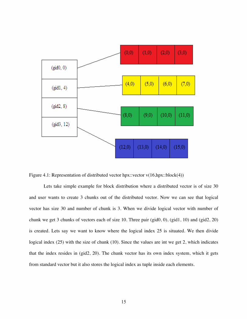
Figure 4.1: Representation of distributed vector hpx::vector v(16,hpx::block(4))

Lets take simple example for block distribution where a distributed vector is of size 30

and user wants to create 3 chunks out of the distributed vector. Now we can see that logical

vector has size 30 and number of chunk is 3. When we divide logical vector with number of

chunk we get 3 chunks of vectors each of size 10. Three pair (gid0, 0), (gid1, 10) and (gid2, 20)

is created. Lets say we want to know where the logical index 25 is situated. We then divide

logical index (25) with the size of chunk (10). Since the values are int we get 2, which indicates

that the index resides in (gid2, 20). The chunk vector has its own index system, which it gets

from standard vector but it also stores the logical index as tuple inside each elements.

16

4.2. Chunk Vector

During the creation of distributed vector the number of chunks divides its total size. This

gives the size of individual chunk of vector, as mentioned in section 4.1. The extra elements that

are left are attached to the last chunk. Chunk Vector uses this size to create a standard vector,

which becomes a part of the logical single vector.

Each elements of chunk vector contains a tuple with pair of int and double value. The int

is for storing the logical index and the double for storing the result of any type of calculation to

be done. The value of logical index in the tuple of chunk vector depends on distribution policy.

Chapel use index set for indexing over the data structure [7]. Further discussion of how index are

placed inside each elements of the chunk vector is discussed in chapter 5. The API of chunk

vector is a wrapper to vector functions. Distributed vector can call these functions synchronously

as well as asynchronously.

Chunk Vector inherits from managed component of HPX. This component is invoked

during the creation of distributed vector, which returns the global id of the object. The number of

components invoked depend on the number of chunk user specifies. If no chunks are specified

the default will be the number of localities. In that case each locality will get a single chunk of

vector. The global id is later used to identify itself and also to pin the chunk vector to certain

locality. Fig 1 shows how the global ids of each chunk vector are collected.

Thus every chunk vector is associated with global id and index. The global id is used for

its identification and index is used for locating where in these chunks of vector does the certain

logical index of the element reside, which is determined mathematically (see example in section

4.1).

17

4.3. Segmented Iterator

The normal iterator of standard template library (STL) iterator concepts is suitable only

for one-dimensional data structure. For its data structure we require the forward iterator to

simply step through the array. A different kind of iterator is required to deal with segmented data

structure. In our case iterator should be aware that while moving forward over the chunk of

vector its successor is next element in the same chunk and if it is at the end of the chunk then the

iterator should move to the beginning of the next chunk.

The segmented iterator holds the information about the global id of current chunk vector

it is pointing to. It also holds the information about the local index of the chunk vector it is

currently pointing to. The iterator when tries to move forward (iterator++) the local index is

increased until it reaches the end of the chunk vector its currently points to. When the end is hit

the iterator goes to the next chunk vector and positioned to the first index of that chunk vector

changing the global id as well.

For random access (iterator + n) it works similarly by increasing the local index and

crossing over the chunk vectors that lies in between.

4.4. Parallel Algorithm

Parallel for_each loop is used for doing computation over the distributed vector. As

parameter it takes:

a. First position of iterator.

b. Last position of iterator.

c. Function object that will be used for computation.

Now the for_each is called over chunks that fall in the iterator range asynchronously.

18

The computation is done over elements of chunk from where the first iterator points to its

end. Then it will include all the chunks that lie between the first and last iterator. Finally, it

includes the chunk, which pointed to the last iterator. Since all the chunks do for_each

asynchronously we could do the computation each of those chunks in parallel.

19

CHAPTER 5. DISTRIBUTION POLICIES

After the respective chunks of vectors have been created by the distributed vector over

there respective localities we have to take care of mapping of the elements of logical vector to

there respective chunks. In this chapter we will explore on how we map elements of logical

vector into those chunks of vectors. We have looked at chapel’s distribution policies [7] and

various other languages [2,3,7], which have provided similar facilities. Distribution policies like

block, cyclic and block-cyclic are provided in chapel to map its index set to respective nodes.

In our distributed vector we use tuple of integer and double value type, where the integer

value type represent the index set and double value type represents the result of computation to

be stored. How these index lay upon those distributed vector is computed arithmetically based on

the distribution policy the vector posses.

Distributing the logical elements in certain fashion for certain problem types produces

statically load balanced distributed vector. For our example we have taken Mandelbrot pixel

calculation (see chapter 6 for more details). In which we calculate each pixel independently.

Some pixel calculation takes more time to complete than other. The pixel along the center of

image takes more computation time then the pixel outside of the center.

In case of Mandelbrot calculation with block distribution where pixels or elements of

logical vector are divided into number of chunks and distributed over the available localities

there is not much of load balancing. But when we do the cyclic distribution of the pixels or

elements of logical vector are distributed over the chunks in round robin fashion. This way each

chunk of vector will get pixel that take longer and pixel that takes short time calculate the result.

This way we could do static load balancing. Also for some cases were there is message passing

20

required between the elements we could choose certain distribution policy, which could reduce

the inter nodal communication.

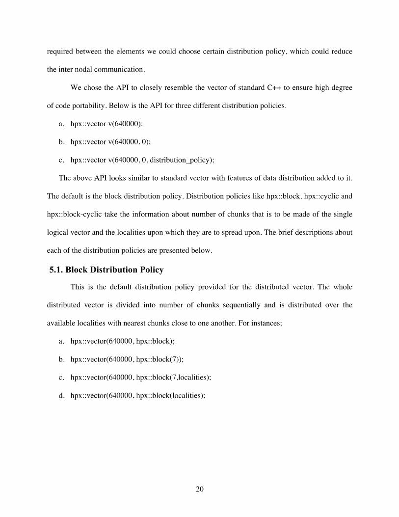
We chose the API to closely resemble the vector of standard C++ to ensure high degree

of code portability. Below is the API for three different distribution policies.

a. hpx::vector v(640000);

b. hpx::vector v(640000, 0);

c. hpx::vector v(640000, 0, distribution_policy);

The above API looks similar to standard vector with features of data distribution added to it.

The default is the block distribution policy. Distribution policies like hpx::block, hpx::cyclic and

hpx::block-cyclic take the information about number of chunks that is to be made of the single

logical vector and the localities upon which they are to spread upon. The brief descriptions about

each of the distribution policies are presented below.

5.1. Block Distribution Policy

This is the default distribution policy provided for the distributed vector. The whole

distributed vector is divided into number of chunks sequentially and is distributed over the

available localities with nearest chunks close to one another. For instances;

a. hpx::vector(640000, hpx::block);

b. hpx::vector(640000, hpx::block(7));

c. hpx::vector(640000, hpx::block(7,localities);

d. hpx::vector(640000, hpx::block(localities);

21

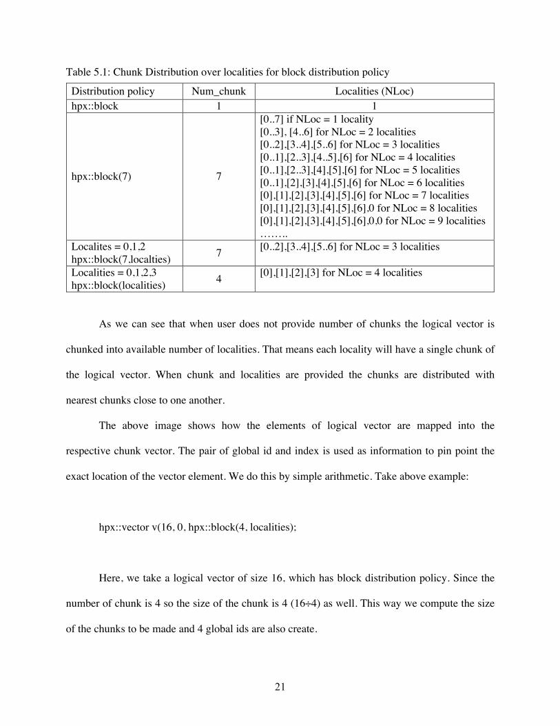
Table 5.1: Chunk Distribution over localities for block distribution policy

As we can see that when user does not provide number of chunks the logical vector is

chunked into available number of localities. That means each locality will have a single chunk of

the logical vector. When chunk and localities are provided the chunks are distributed with

nearest chunks close to one another.

The above image shows how the elements of logical vector are mapped into the

respective chunk vector. The pair of global id and index is used as information to pin point the

exact location of the vector element. We do this by simple arithmetic. Take above example:

hpx::vector v(16, 0, hpx::block(4, localities);

Here, we take a logical vector of size 16, which has block distribution policy. Since the

number of chunk is 4 so the size of the chunk is 4 (16÷4) as well. This way we compute the size

of the chunks to be made and 4 global ids are also create.

Distribution policy Num_chunk Localities (NLoc) hpx::block 1 1

hpx::block(7) 7

[0..7] if NLoc = 1 locality [0..3], [4..6] for NLoc = 2 localities [0..2],[3..4],[5..6] for NLoc = 3 localities [0..1],[2..3],[4..5],[6] for NLoc = 4 localities [0..1],[2..3],[4],[5],[6] for NLoc = 5 localities [0..1],[2],[3],[4],[5],[6] for NLoc = 6 localities [0],[1],[2],[3],[4],[5],[6] for NLoc = 7 localities [0],[1],[2],[3],[4],[5],[6],0 for NLoc = 8 localities [0],[1],[2],[3],[4],[5],[6],0,0 for NLoc = 9 localities ……..

Localites = 0,1,2 hpx::block(7,localties) 7 [0..2],[3..4],[5..6] for NLoc = 3 localities

Localities = 0,1,2,3 hpx::block(localities) 4 [0],[1],[2],[3] for NLoc = 4 localities

22

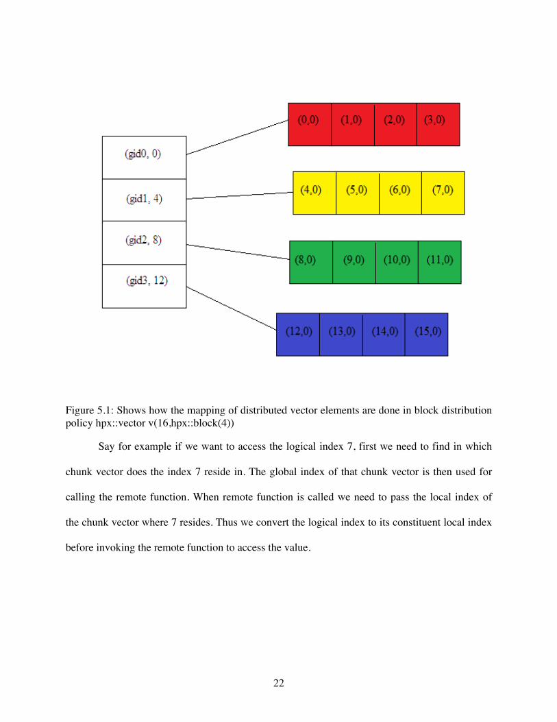
Figure 5.1: Shows how the mapping of distributed vector elements are done in block distribution policy hpx::vector v(16,hpx::block(4))

Say for example if we want to access the logical index 7, first we need to find in which

chunk vector does the index 7 reside in. The global index of that chunk vector is then used for

calling the remote function. When remote function is called we need to pass the local index of

the chunk vector where 7 resides. Thus we convert the logical index to its constituent local index

before invoking the remote function to access the value.

23

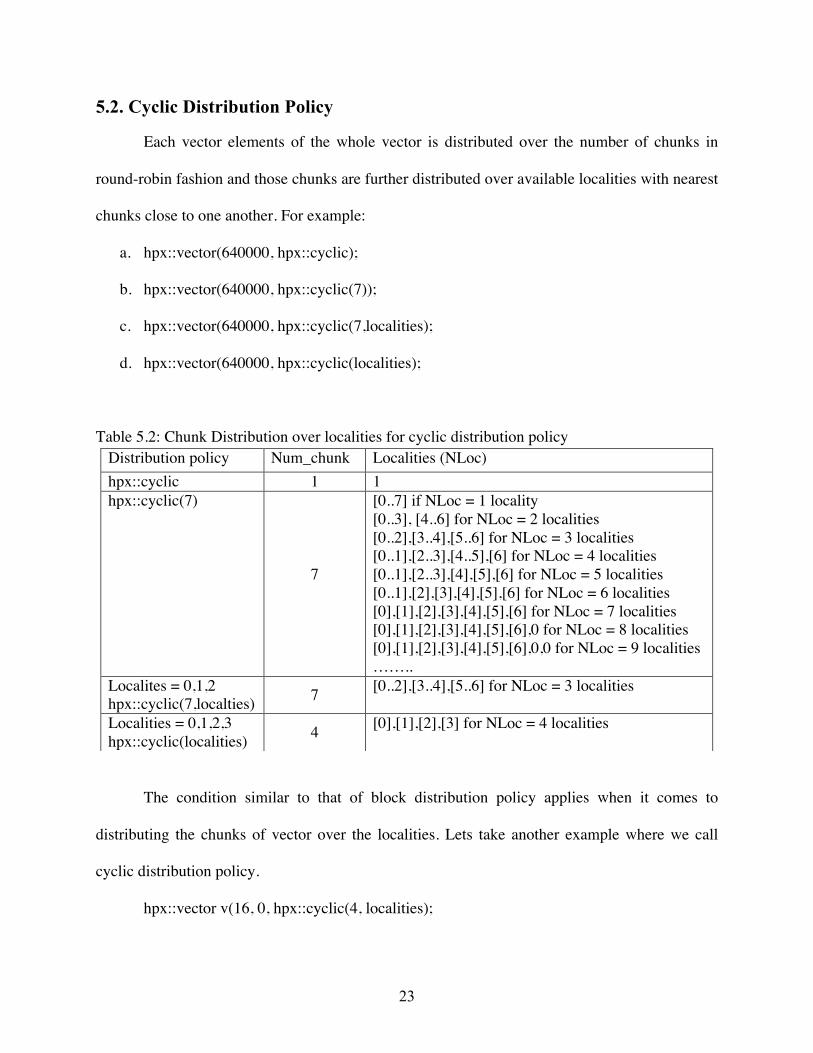
5.2. Cyclic Distribution Policy

Each vector elements of the whole vector is distributed over the number of chunks in

round-robin fashion and those chunks are further distributed over available localities with nearest

chunks close to one another. For example:

a. hpx::vector(640000, hpx::cyclic);

b. hpx::vector(640000, hpx::cyclic(7));

c. hpx::vector(640000, hpx::cyclic(7,localities);

d. hpx::vector(640000, hpx::cyclic(localities);

Table 5.2: Chunk Distribution over localities for cyclic distribution policy

The condition similar to that of block distribution policy applies when it comes to

distributing the chunks of vector over the localities. Lets take another example where we call

cyclic distribution policy.

hpx::vector v(16, 0, hpx::cyclic(4, localities);

Distribution policy Num_chunk Localities (NLoc) hpx::cyclic 1 1 hpx::cyclic(7)

7


Localites = 0,1,2 hpx::cyclic(7,localties) 7 [0..2],[3..4],[5..6] for NLoc = 3 localities

Localities = 0,1,2,3 hpx::cyclic(localities) 4 [0],[1],[2],[3] for NLoc = 4 localities

24

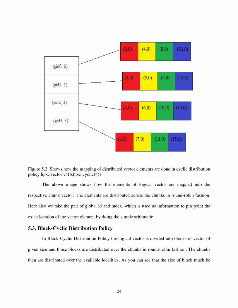
Figure 5.2: Shows how the mapping of distributed vector elements are done in cyclic distribution policy hpx::vector v(16,hpx::cyclic(4))

The above image shows how the elements of logical vector are mapped into the

respective chunk vector. The elements are distributed across the chunks in round-robin fashion.

Here also we take the pair of global id and index, which is used as information to pin point the

exact location of the vector element by doing the simple arithmetic.

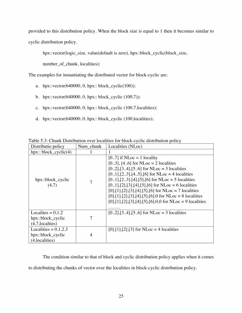
5.3. Block-Cyclic Distribution Policy

In Block-Cyclic Distribution Policy the logical vector is divided into blocks of vector of

given size and those blocks are distributed over the chunks in round-robin fashion. The chunks

then are distributed over the available localities. As you can see that the size of block much be

25

provided to this distribution policy. When the block size is equal to 1 then it becomes similar to

cyclic distribution policy.

hpx::vector(logic_size, value(default is zero), hpx::block_cyclic(block_size,

number_of_chunk, localities);

The examples for instantiating the distributed vector for block-cyclic are:

a. hpx::vector(640000, 0, hpx:: block_cyclic(100));

b. hpx::vector(640000, 0, hpx:: block_cyclic (100,7));

c. hpx::vector(640000, 0, hpx:: block_cyclic (100,7,localities);

d. hpx::vector(640000, 0, hpx:: block_cyclic (100,localities);

Table 5.3: Chunk Distribution over localities for block-cyclic distribution policy Distributio policy Num_chunk Localities (NLoc) hpx:: block_cyclic(4) 1 1

hpx::block_cyclic (4,7) 7


Localites = 0,1,2 hpx::block_cyclic (4,7,localties)

7 [0..2],[3..4],[5..6] for NLoc = 3 localities

Localities = 0,1,2,3 hpx::block_cyclic (4,localities)

4 [0],[1],[2],[3] for NLoc = 4 localities

The condition similar to that of block and cyclic distribution policy applies when it comes

to distributing the chunks of vector over the localities in block-cyclic distribution policy.

26

Figure 5.3: Shows how the mapping of distributed vector elements are done in block-cyclic distribution policy hpx::vector v(16,hpx::block_cyclic(2,4))

Lets take and example of block-cyclic:

hpx::vector v(16, 0, hpx:: block_cyclic (2, 4, localities));

The above example is depicted in the image of figure 5.3. As you can see the block_size

is 2, which is the size that is used to make block size of two, then this block is distributed in

round-robin fashion four chunks of vectors.

27

CHAPTER 6. EXPERIMENTS AND RESULTS

In this chapter we will implement our distributed vector using different distribution

policy to compute the Mandelbrot Pixel. The image of a Mandelbrot set is drawn on complex

plane, which has real values on the x-axis and imaginary values on the y-axis. Thus, each point

on the graph represents a complex number C where 𝐶 = 𝐶! + 𝐶!𝑖 or (𝐶! ,𝐶!). Each point has a

pixel value, which is determined by the number of iterations (n) it takes to make the sequences of

Z’s absolute value where 𝑍 = 𝑍! + 𝑍!𝑖 or (𝑍! ,𝑍!), to be greater than or equal to two. The

absolute value of a complex number is equivalent to the distance from 0 to Z in the complex

plane. Z is calculated by:

𝑍!!! = 𝑍!! + 𝐶

These calculations are preformed inside the function object. First the local variables are

initialized: 𝑍! 𝑎𝑠 𝑍! = 0 𝑎𝑛𝑑 𝑍! = 0. Next the loop checks to see if the absolute value of Z is

greater than or equal to 2. The value of the next Z is then calculated. Since some of these

iterations converge to infinity, I have chosen max iteration to be certain high constant (400). The

while loop also checks to see if it has crossed the max iteration. Finally, the loop exits and

returns the number of iterations in the loop, which is latter used as a pixel color in the

Mandelbrot set image.

The algorithm for the Mandelbrot pixel calculation shows how the iterator returns the

tuple and we use the information in this tuple to calculate the co-ordinates which is later use for

computation.

28

// Does the pixel calculation struct mandelbrot { void operator () (std::tuple<int, double>& t ) { double Zr , Zr, temp= 0.0; int times = 0; int x0 = std::get<0>(t)%Size_X; int y0 = std::get<0>(t)/Size_Y; double Cr = (double)(x0)*3.500/(double)Size_X-2.500; double Ci = (double)(y0)*2.000/(double)Size_Y-1.000; Zr = Zr+Cr; Zi = Zi+Ci; while ((((Zr*Zr)+(Zi*Zi))<=4) && (times < maxiteration)) { temp = (Zr*Zr)-(Zi*Zi); Zi = 2*Zr*Zi; Zr = temp+Cr; Zi = Zi+Ci; times = times+1; } std::get<1>(t) = times; } }mandel;

The computation is done through parallel for_each loop, which does the computation

over each of the chunks in parallel. The iterator returns tuple of index and value since each of the

elements of our distributed vector contains this tuple. The information about the index is used to

calculate the Cartesian co-ordinate of the complex plane. The function object to compute the

pixel then uses this co-ordinate.

Eg:

a. hpx::vector v(640000, hpx::block(800, localities);

b. hpx::for_each(v.begin(), v.end() , mandel);

29

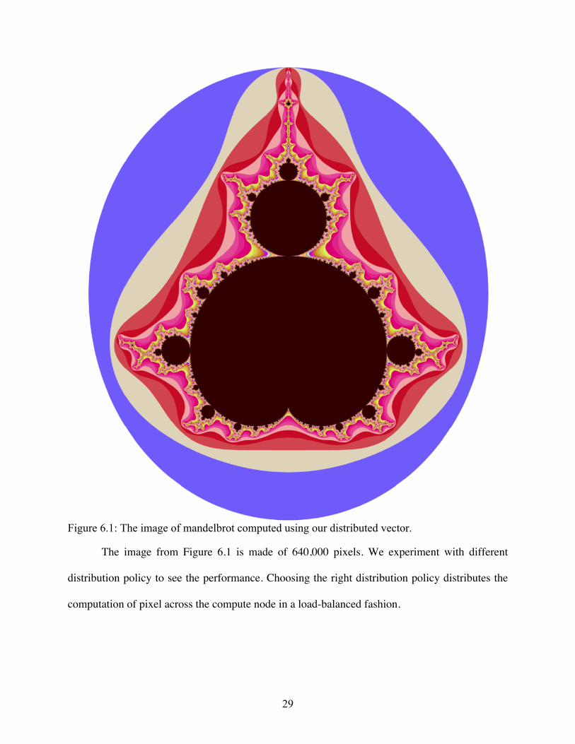
Figure 6.1: The image of mandelbrot computed using our distributed vector.

The image from Figure 6.1 is made of 640,000 pixels. We experiment with different

distribution policy to see the performance. Choosing the right distribution policy distributes the

computation of pixel across the compute node in a load-balanced fashion.

30

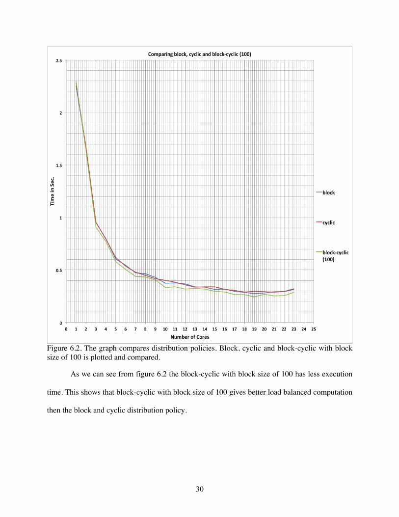
Figure 6.2. The graph compares distribution policies. Block, cyclic and block-cyclic with block size of 100 is plotted and compared.

As we can see from figure 6.2 the block-cyclic with block size of 100 has less execution

time. This shows that block-cyclic with block size of 100 gives better load balanced computation

then the block and cyclic distribution policy.

31

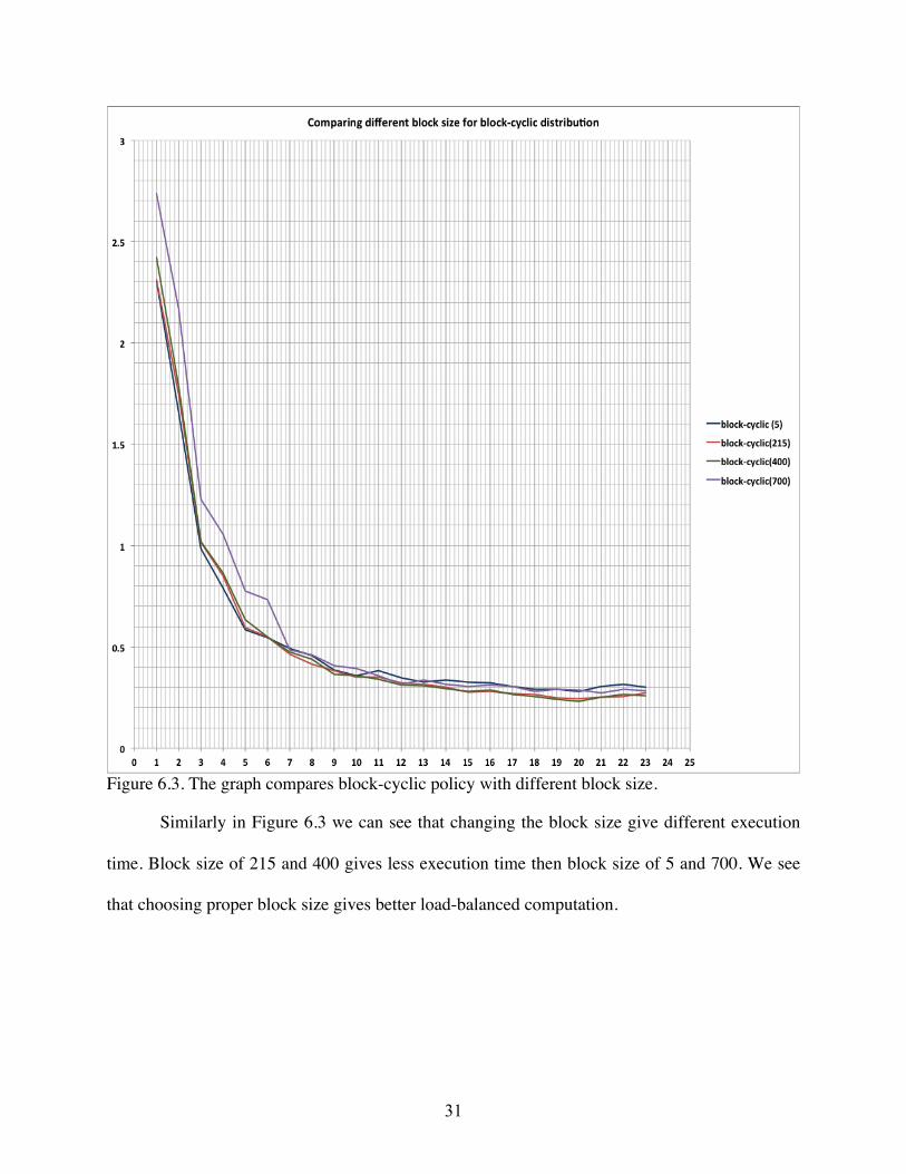
Figure 6.3. The graph compares block-cyclic policy with different block size.

Similarly in Figure 6.3 we can see that changing the block size give different execution

time. Block size of 215 and 400 gives less execution time then block size of 5 and 700. We see

that choosing proper block size gives better load-balanced computation.

32

CHAPTER 7. CONCLUSION

In this thesis we have designed and implemented distributed vector and API for the data

distribution policy. We added tuple of index and values to each element of vectors. We showed

how we could use our API for hiding the internal details of data distribution in HPX. Similarly

we can also say that choosing the right distribution policy we can do the static load balancing.

For the Mandelbrot pixel calculation we can use block-cyclic to distribute pixel in certain fashion

that would have collection of pixels from different part of the image. This would eventually give

load-balanced distribution of pixel computation.

In future we could implement dynamic load balancing by migrating the individual chunk

to particular locality during runtime.

33

CHAPTER 8. REFERENCES

1. Espasa, R., Valero, M., & Smith, J. E. (1998, July). Vector architectures: past, present and future. In Proceedings of the 12th international conference on Supercomputing (pp. 425-432). ACM.

2. Kennedy, K., Koelbel, C., & Zima, H. (2007, June). The rise and fall of High Performance Fortran: an historical object lesson. In Proceedings of the third ACM SIGPLAN conference on History of programming languages (pp. 7-1). ACM.

3. Mehrotra, P., & Van Rosendale, J. (1990). Programming distributed memory architectures using Kali (No. ICASE-90-69). INSTITUTE FOR COMPUTER APPLICATIONS IN SCIENCE AND ENGINEERING HAMPTON VA.

4. Kaiser, H., Brodowicz, M., & Sterling, T. (2009, September). Parallex an advanced parallel execution model for scaling-impaired applications. In Parallel Processing Workshops, 2009. ICPPW'09. International Conference on (pp. 394-401). IEEE.

5. Habraken, J. Adding capability-based security to High Performance ParalleX.

6. Austern, M. H. (2000). Segmented iterators and hierarchical algorithms. InGeneric Programming (pp. 80-90). Springer Berlin Heidelberg.

7. Diaconescu, R. E., & Zima, H. P. (2007). An approach to data distributions in Chapel. International Journal of High Performance Computing Applications,21(3), 313-335.

8. Kaiser, H., Heller, T., Adelstein-Lelbach, B., Serio, A., & Fey, D. HPX–A Task Based Programming Model in a Global Address Space.

9. Yelick, K., Bonachea, D., Chen, W. Y., Colella, P., Datta, K., Duell, J., ... & Wen, T. (2007, July). Productivity and performance using partitioned global address space languages. In Proceedings of the 2007 international workshop on Parallel symbolic computation (pp. 24-32). ACM.

10. Kale, L. V., & Krishnan, S. (1993). CHARM++: a portable concurrent object oriented system based on C++ (Vol. 28, No. 10, pp. 91-108). ACM.

11. Nieplocha, J., Palmer, B., Tipparaju, V., Krishnan, M., Trease, H., & Aprà, E. (2006). Advances, applications and performance of the global arrays shared memory programming toolkit. International Journal of High Performance Computing Applications, 20(2), 203-231.

12. Nieplocha, J., & Carpenter, B. (1999). ARMCI: A portable remote memory copy library for distributed array libraries and compiler run-time systems. In Parallel and Distributed Processing (pp. 533-546). Springer Berlin Heidelberg.

34

13. Fox, G., Hiranandani, S., Kennedy, K., Koelbel, C., Kremer, U., Tseng, C. W., & Wu, M. Y. (1990). Fortran D language specification.

14. Chamberlain, B. L., Callahan, D., & Zima, H. P. (2007). Parallel programmability and the chapel language. International Journal of High Performance Computing Applications, 21(3), 291-312.

35

VITA

Bibek Ghimire was born in Pokhara-10, Nepal. He received his Bachelor’s degree in

Computer Science from Louisiana State University, Baton Rouge, USA in 2012. Then he joined

Department Electrical Engineering and Computer Science in Louisiana State University, Baton

Rouge, USA in 2012 for his Master’s degree in System Science. He is expected to graduate in

December 2014.

Documents

DATA DISTRIBUTION IN HPX