Embed Size (px)
DESCRIPTION
Data-Driven Decision-Making The Good, the Bad, and the Ugly Ruda Kulhav ý Honeywell International, Inc. Automation and Control Solutions Advanced Technology. Can We Generate More Value from Data?. - PowerPoint PPT Presentation
Citation preview

Data-Driven Decision-MakingData-Driven Decision-Making
The Good, the Bad, and the UglyThe Good, the Bad, and the Ugly
Ruda Kulhavý
Honeywell International, Inc.Automation and Control Solutions
Advanced Technology

Can We Generate More Value from Data?Can We Generate More Value from Data?
Today, a typical “data mining” project is ad hoc, lengthy, costly, knowledge-intensive, and requiring on-going maintenance.
Although the project benefits can be quite significant, the resulting profit is often marginalthe resulting profit is often marginal.
The industry is in search of robust methods and robust methods and reusable workflowsreusable workflows, easy to use and adapteasy to use and adapt to system and organizational changes, and requiring requiring no special knowledgeno special knowledge from the end user.
This is a tough target … What can we offer to it today?
Learning from DataLearning from Data
Probabilistic Approach Probabilistic Approach
Learning from DataLearning from Data
Probabilistic Approach Probabilistic Approach
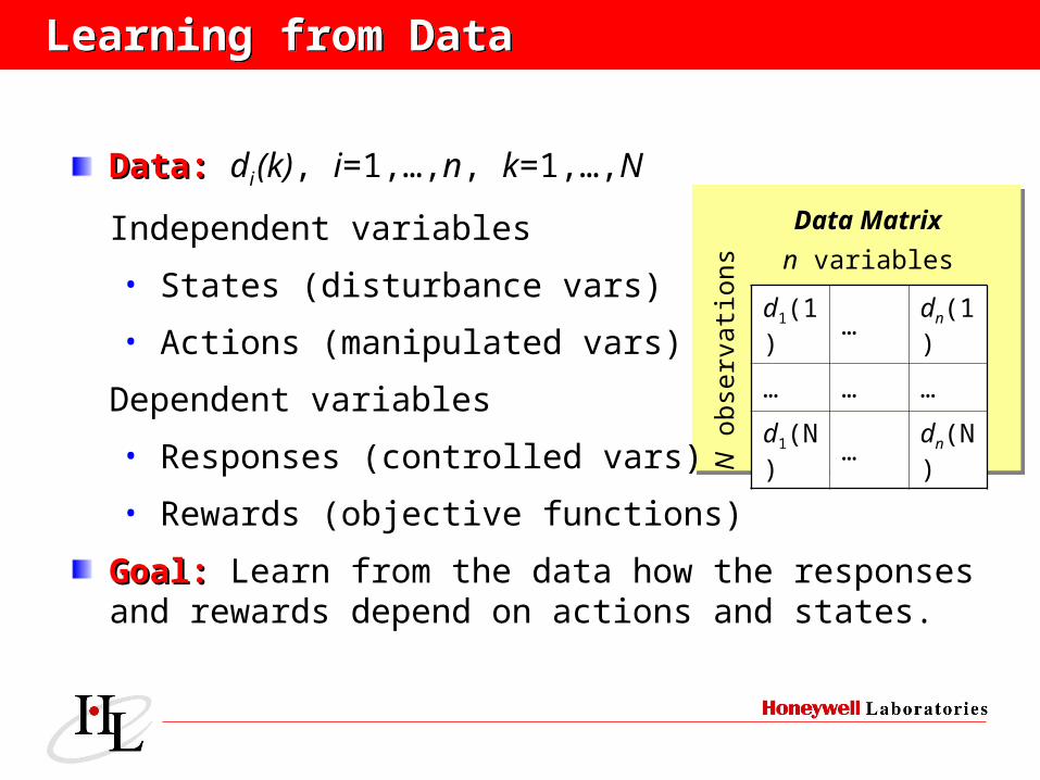
Learning from DataLearning from Data
Data:Data: di (k), i=1,…,n, k=1,…,N
Independent variables
• States (disturbance vars)
• Actions (manipulated vars)
Dependent variables
• Responses (controlled vars)
• Rewards (objective functions)
Goal:Goal: Learn from the data how the responses and rewards depend on actions and states.
d1(1)
…dn(1)
… … …
d1(N)
…dn(N)
n variables
N o
bse
rvati
ons
Data Matrix
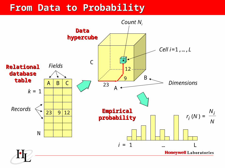
From Data to ProbabilityFrom Data to Probability
A
B
C
239
12
DataDatahypercubehypercube
Cell i =1,…,L
Dimensions
Count Ni
A B C
23 9 12
Fields
Records
RelationalRelationaldatabasedatabase
tabletable
k = 1
N
i = 1 … L
N
NNr i
i =)(EmpiricalEmpirical
probabilityprobability
Smoothenedprobability
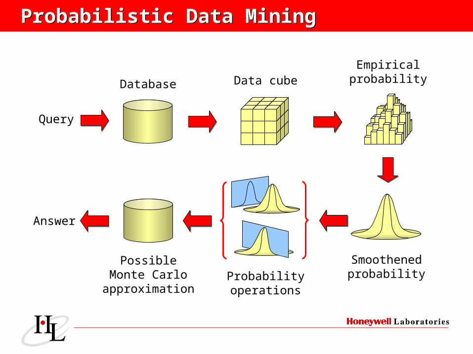
Data cubeDatabase
Query
Empiricalprobability
Probabilityoperations
PossibleMonte Carlo
approximation
Answer
Probabilistic Data MiningProbabilistic Data Mining
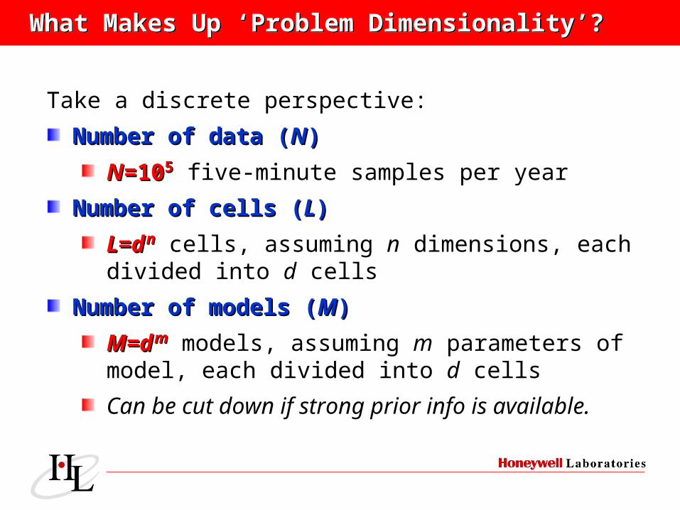
What Makes Up ‘Problem Dimensionality’?What Makes Up ‘Problem Dimensionality’?
Take a discrete perspective:
Number of data (Number of data (NN))
NN=10=1055 five-minute samples per year
Number of cells (Number of cells (LL))
L=dL=d nn cells, assuming n dimensions, each
divided into d cells
Number of models (Number of models (MM))
M=dM=d mm models, assuming m parameters of
model, each divided into d cells
Can be cut down if strong prior info is available.
Addressing DimensionalityAddressing Dimensionality
Macroscopic PredictionMacroscopic Prediction
Addressing DimensionalityAddressing Dimensionality
Macroscopic PredictionMacroscopic Prediction
Macroscopic PredictionMacroscopic Prediction
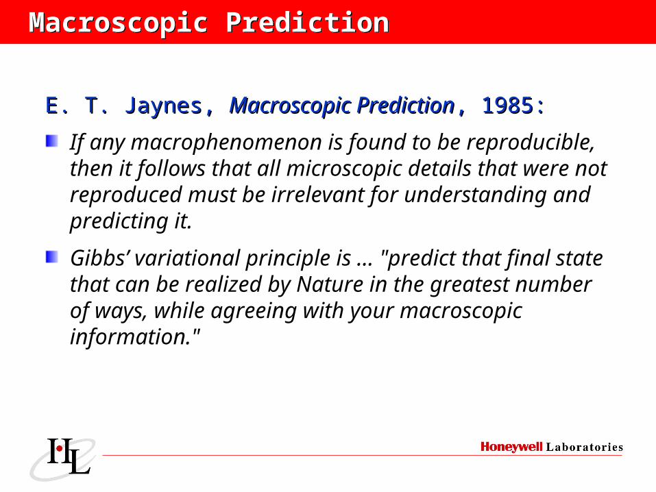
E. T. Jaynes, E. T. Jaynes, Macroscopic PredictionMacroscopic Prediction, 1985:, 1985:
If any macrophenomenon is found to be reproducible, then it follows that all microscopic details that were not reproduced must be irrelevant for understanding and predicting it.
Gibbs’ variational principle is … "predict that final state that can be realized by Nature in the greatest number of ways, while agreeing with your macroscopic information."
Boltzmann’s Solution (1877)Boltzmann’s Solution (1877)
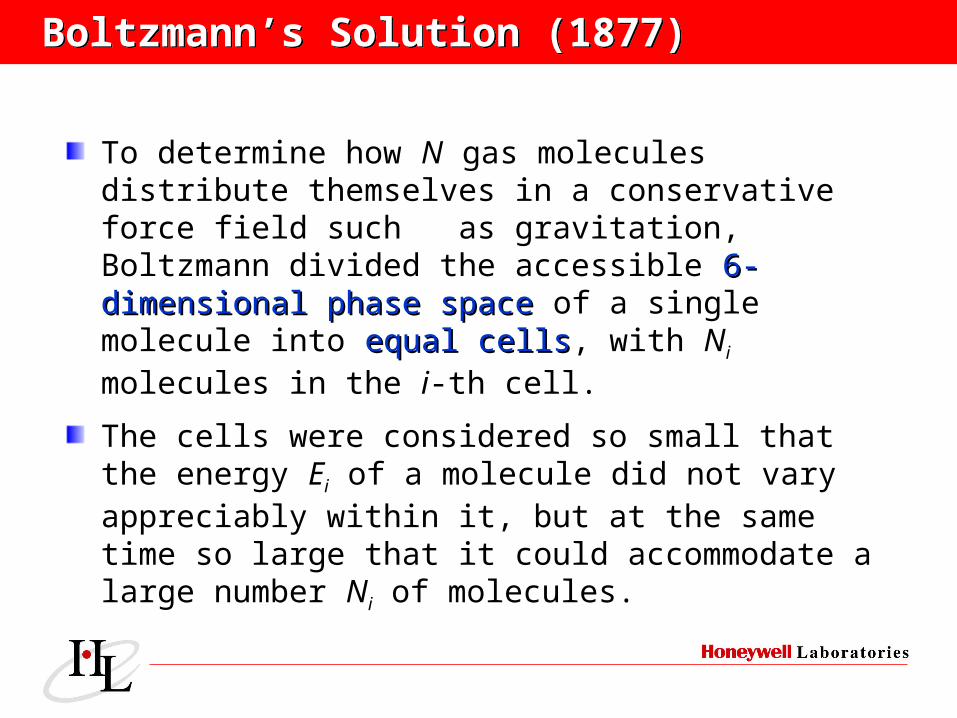
To determine how N gas molecules distribute themselves in a conservative force field such as gravitation, Boltzmann divided the accessible 6-dimensional phase space6-dimensional phase space of a single molecule into equal cellsequal cells, with Ni molecules in the i-th cell.
The cells were considered so small that the energy Ei of a molecule did not vary appreciably within it, but at the same time so large that it could accommodate a large number Ni of molecules.
Boltzmann’s Solution (cont.)Boltzmann’s Solution (cont.)
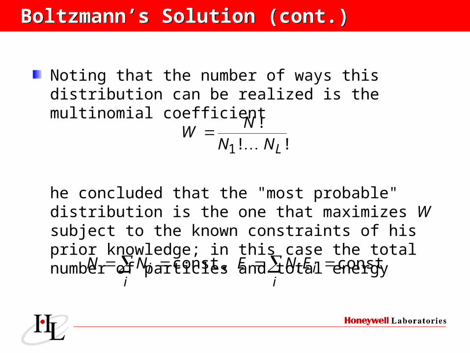
Noting that the number of ways this distribution can be realized is the multinomial coefficient
he concluded that the "most probable" distribution is the one that maximizes W subject to the known constraints of his prior knowledge; in this case the total number of particles and total energy
!!!
1 LNNN
W
const.,const. ii
ii
i ENENN
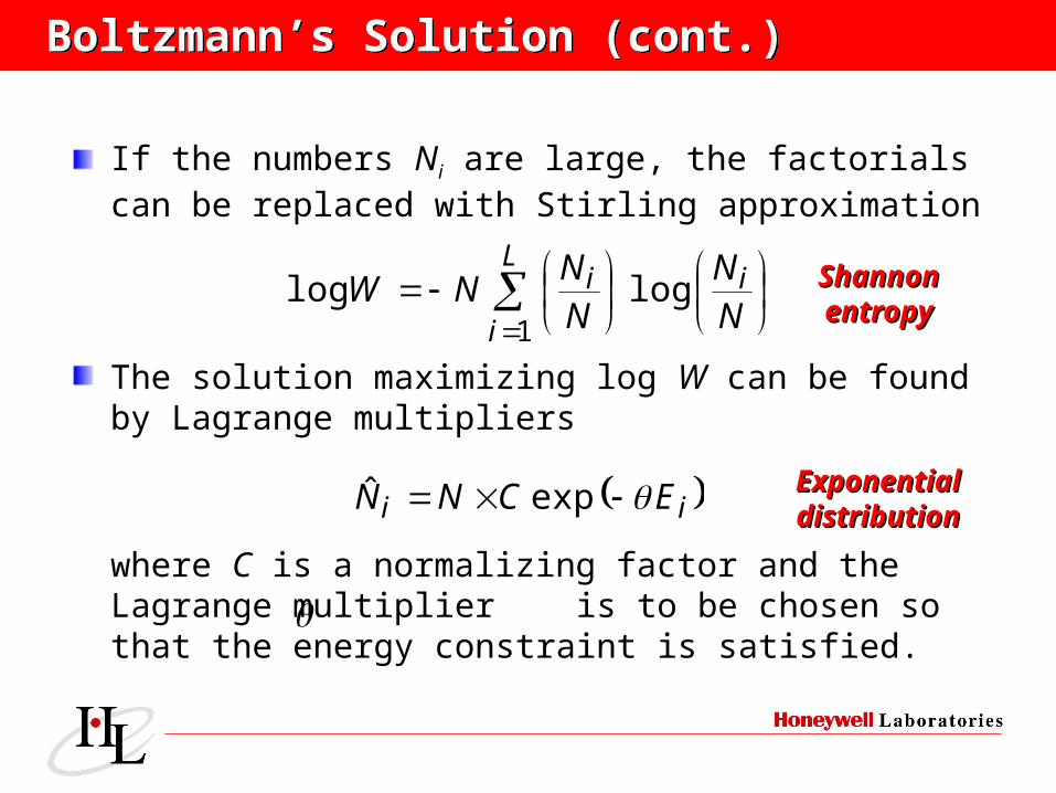
If the numbers Ni are large, the factorials can be replaced with Stirling approximation
The solution maximizing log W can be found by Lagrange multipliers
where C is a normalizing factor and the Lagrange multiplier is to be chosen so that the energy constraint is satisfied.
Boltzmann’s Solution (cont.)Boltzmann’s Solution (cont.)
NN
NN
NW iL
i
i loglog1
ii ECNN expˆ
ShannonShannonentropyentropy
ExponentialExponentialdistributiondistribution
Why Does It Work?Why Does It Work?
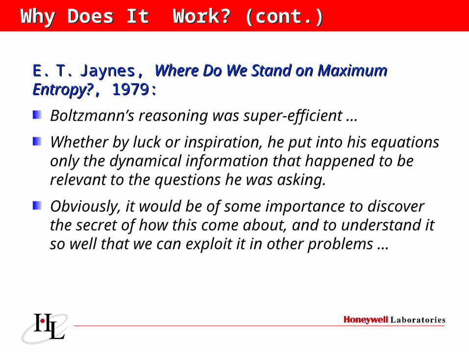
E.E. T.T. Jaynes, Jaynes, Where Do We Stand on MaximumWhere Do We Stand on MaximumEntropy?Entropy?, 1979:, 1979:
Information about the dynamics entered Boltzmann’s equations at two places: (1) the conservation of total energy; and (2) the fact that he defined his cells in terms of phase volume …
The fact that this was enough to predict the correct spatial and velocity distribution of the molecules shows that the millions of intricate dynamical details that were not taken into account, were actually irrelevant to the predictions …
Why Does It Work? (cont.) Why Does It Work? (cont.)
E.E. T.T. Jaynes, Jaynes, Where Do We Stand on MaximumWhere Do We Stand on MaximumEntropy?Entropy?, 1979:, 1979:
Boltzmann’s reasoning was super-efficient …
Whether by luck or inspiration, he put into his equations only the dynamical information that happened to be relevant to the questions he was asking.
Obviously, it would be of some importance to discover the secret of how this come about, and to understand it so well that we can exploit it in other problems …
General Maximum EntropyGeneral Maximum Entropy
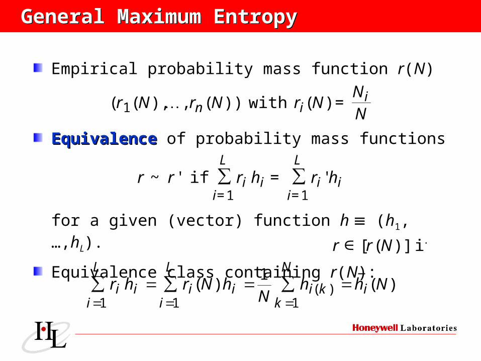
Empirical probability mass function r(N)
EquivalenceEquivalence of probability mass functions
for a given (vector) function h (h1,…,hL).
Equivalence class containing r(N):
NN
NrNrNr iin =)(with))(,),(( 1
∑∑L
iii
L
iii hrhrrr
1=1='=if'~
)(1
)(1
)(11
NhhN
hNrhr i
N
kki
L
iii
L
iii
∑∑∑
if)]([ Nrr ∈
General Maximum Entropy (cont.)General Maximum Entropy (cont.)
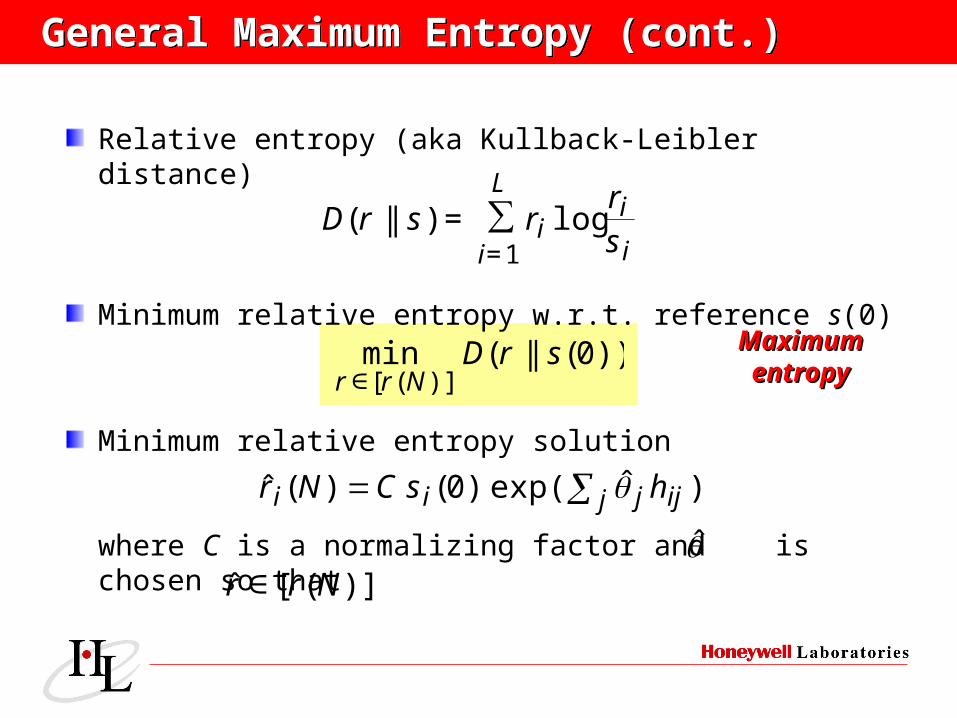
Relative entropy (aka Kullback-Leibler distance)
Minimum relative entropy w.r.t. reference s(0)
Minimum relative entropy solution
where C is a normalizing factor and is chosen so that
))0(||(min)]([
srDNrr ∈
∑L
i i
ii s
rrsrD
1=log=)||(
)ˆexp()0()(ˆ j ijjii hsCNr
)].([ˆ Nrr ∈
MaximumMaximumentropyentropy
Addressing DimensionalityAddressing Dimensionality
Parametric ApproximationParametric Approximation
Addressing DimensionalityAddressing Dimensionality
Parametric ApproximationParametric Approximation
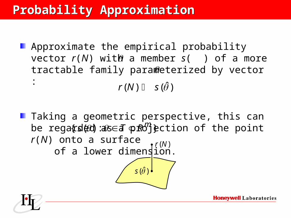
Probability ApproximationProbability Approximation
Approximate the empirical probability vector r(N) with a member s( ) of a more tractable family parameterized by vector :
Taking a geometric perspective, this can be regarded as a projection of the point r(N) onto a surface of a lower dimension.
)ˆ()( sNr
}:)({ mRTs )(Nr
)ˆ(s
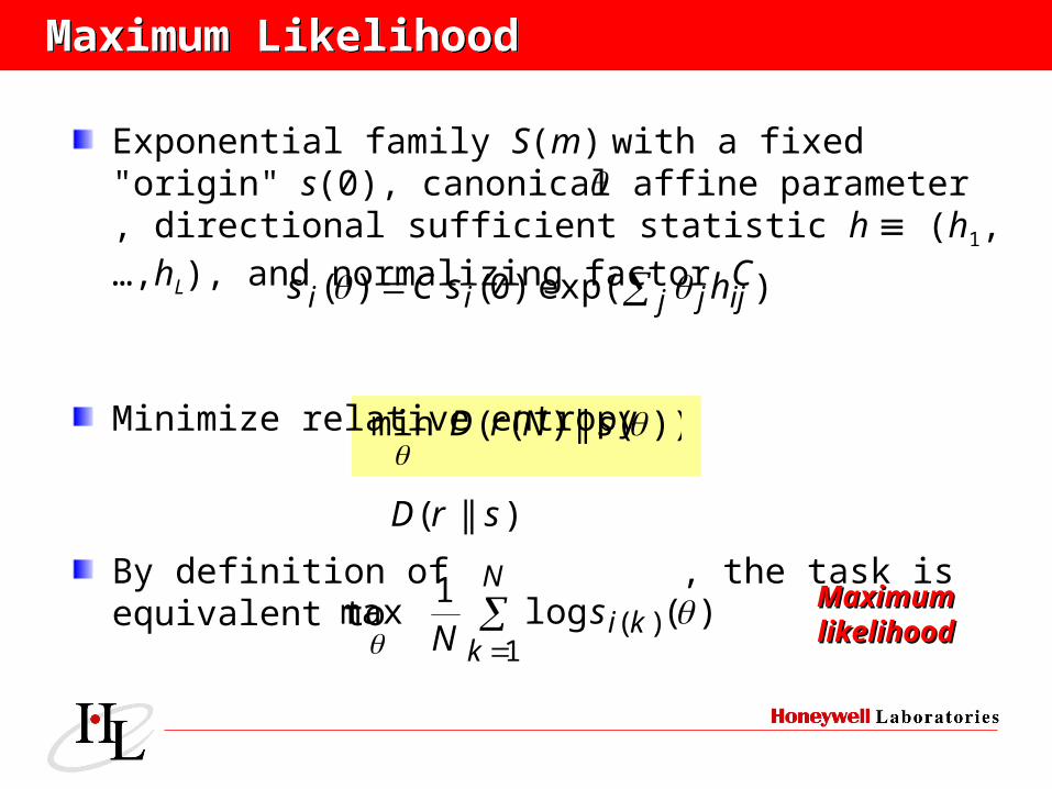
Maximum LikelihoodMaximum Likelihood
Exponential family S(m) with a fixed "origin" s(0), canonical affine parameter , directional sufficient statistic h (h1,…,hL), and normalizing factor C
Minimize relative entropy
By definition of , the task is equivalent to
)exp()0()( j ijjii hsCs
))(||)((min
sNrD
MaximumMaximumlikelihoodlikelihood
N
kkis
N 1)( )(log
1max
)||( srD
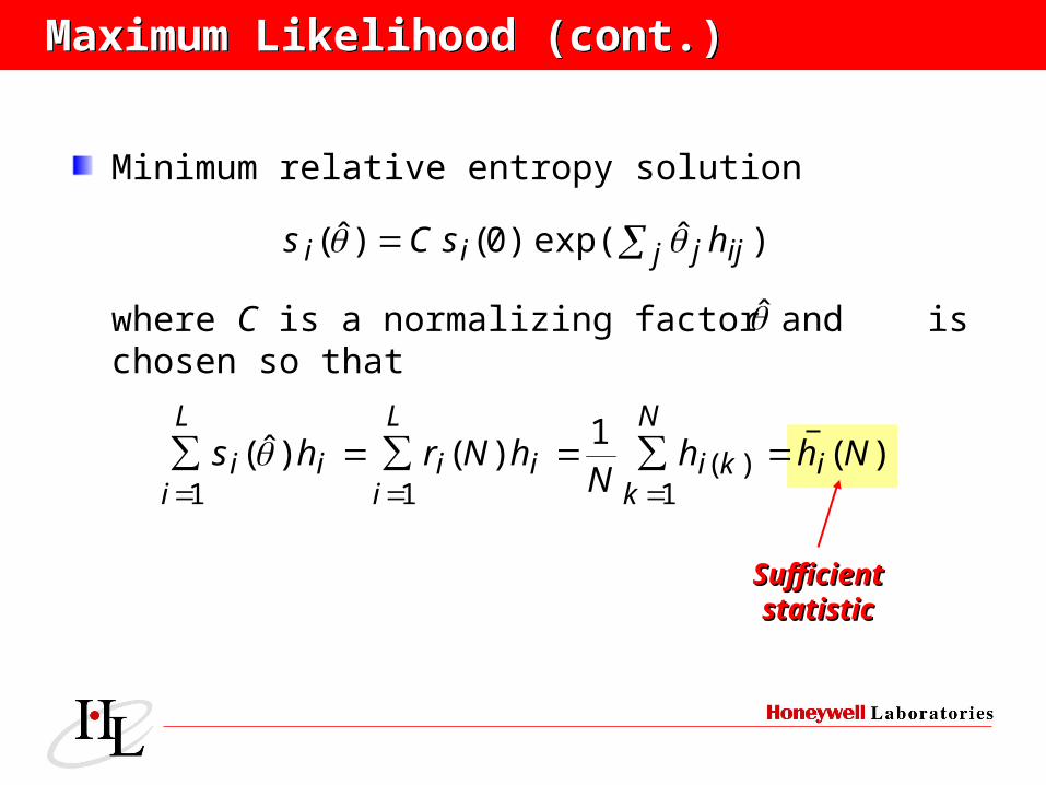
Maximum Likelihood (cont.)Maximum Likelihood (cont.)
Minimum relative entropy solution
where C is a normalizing factor and is chosen so that
)(1
)()ˆ(1
)(11
NhhN
hNrhs i
N
kki
L
iii
L
iii
∑∑∑
SufficientSufficientstatisticstatistic
)ˆexp()0()ˆ( j ijjii hsCs

Addressing DimensionalityAddressing Dimensionality
Information GeometryInformation Geometry
Addressing DimensionalityAddressing Dimensionality
Information GeometryInformation Geometry
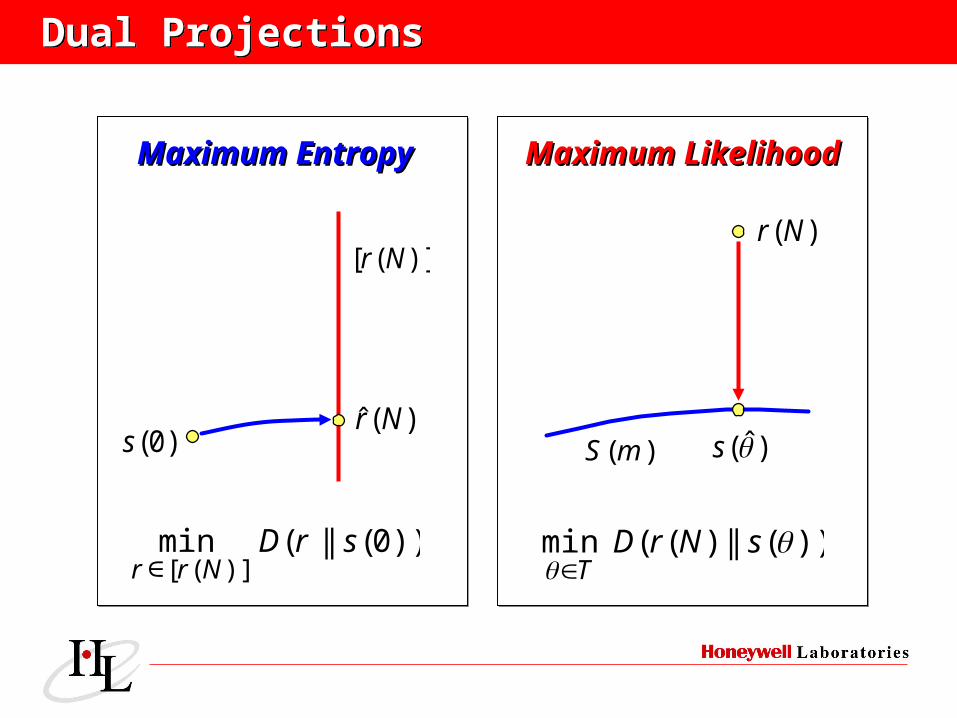
Dual ProjectionsDual Projections
)(Nr
)ˆ(s)(mS
))(||)((min
sNrDT
Maximum LikelihoodMaximum Likelihood
)0(s)(ˆ Nr
)]([ Nr
))0(||(min)]([
srDNrr ∈
Maximum EntropyMaximum Entropy
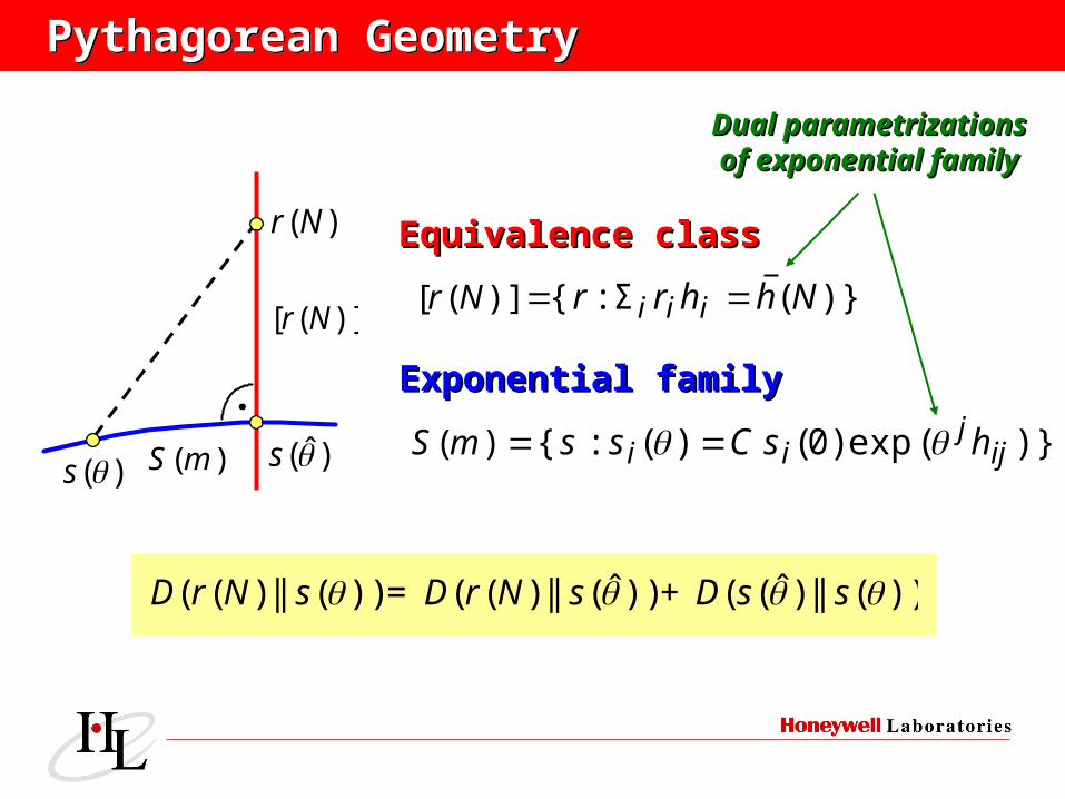
Pythagorean GeometryPythagorean Geometry
)(s
)(Nr
Exponential familyExponential family
Equivalence classEquivalence class
)ˆ(s
))(||)ˆ((+))ˆ(||)((=))(||)(( ssDsNrDsNrD
)}(exp)0()(:{)( ijj
ii hsCssmS
)]([ Nr
)(mS
)}(Σ:{)]([ Nhhrr iiiNr
Dual parametrizationsDual parametrizationsof exponential familyof exponential family
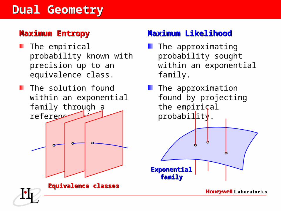
Dual Geometry Dual Geometry
Maximum EntropyMaximum Entropy
The empirical probability known with precision up to an equivalence class.
The solution found within an exponential family through a reference point.
Maximum LikelihoodMaximum Likelihood
The approximating probability sought within an exponential family.
The approximation found by projecting the empirical probability.
Equivalence classesEquivalence classes
ExponentialExponentialfamilyfamily
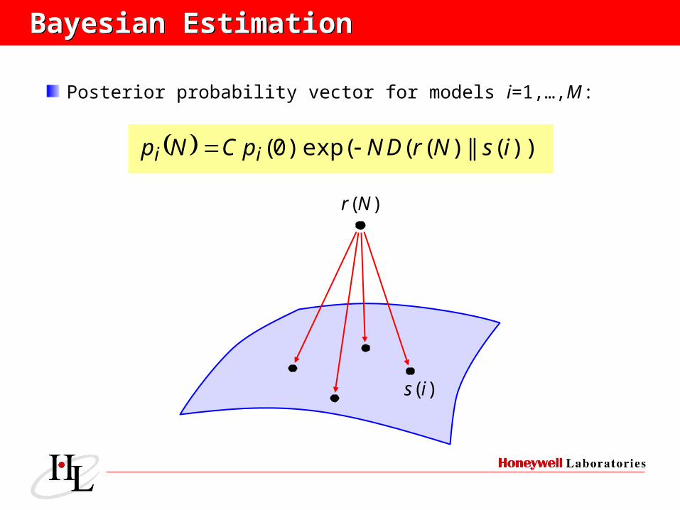
Bayesian EstimationBayesian Estimation
Posterior probability vector for models i=1,…,M :
)))(||)((exp()0( isNrDNpCNp ii
)(Nr
)(is
Addressing DimensionalityAddressing Dimensionality
Relevance-Based WeightingRelevance-Based Weighting
Addressing DimensionalityAddressing Dimensionality
Relevance-Based WeightingRelevance-Based Weighting
What If the Model Is Too Complex?What If the Model Is Too Complex?
For some real-life problems, the level of detail that needs to be collected on the empirical probability (and, correspondingly, the dimension of the exponential family) is too high, possibly infinite.In such case, we can either
sacrifice the closed-form solution, ortake a narrower view of the data, • modeling only the part of system behavior modeling only the part of system behavior
relevant to the problem in questionrelevant to the problem in question, • while using a simpler, lower-dimensional while using a simpler, lower-dimensional
modelmodel.
Relevance-Based Weighting of DataRelevance-Based Weighting of Data
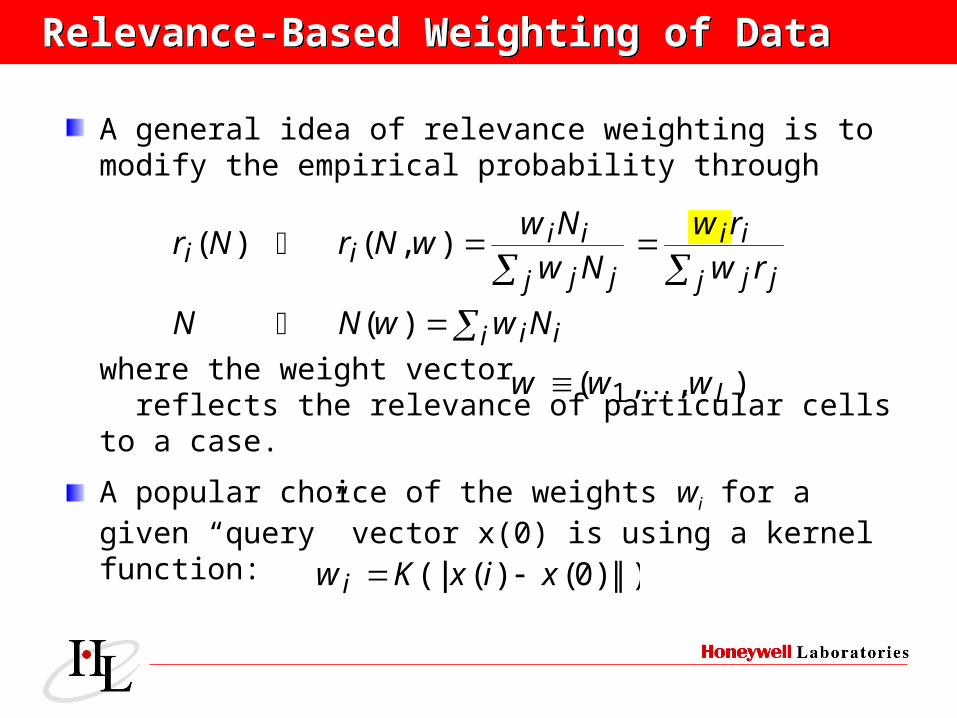
A general idea of relevance weighting is to modify the empirical probability through
where the weight vector reflects the relevance of particular cells to a case.
A popular choice of the weights wi for a given “query” vector x(0) is using a kernel function:
i ii
j jj
ii
j jj
iiii
NwwNN
rwrw
NwNw
wNrNr
)(
),()(
),,( 1 Lwww
|)|)0()(|(| xixKwi
Local Empirical DistributionsLocal Empirical DistributionsR
esp
onse
vari
able
Predictor variable
)(ˆ 1ws
)(ˆ 2ws)(ˆ 3ws
)( 1wr)( 2wr )( 3wr
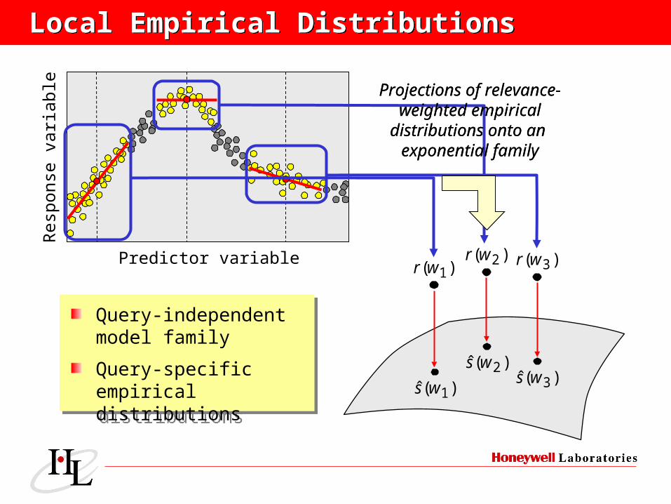
Projections of relevance-weighted empirical
distributions onto an exponential family
Query-independent model family
Query-specific empirical distributions
Query-independent model family
Query-specific empirical distributions
Projections of relevance-weighted empirical
distributions onto an exponential family
Local ModelingLocal Modeling
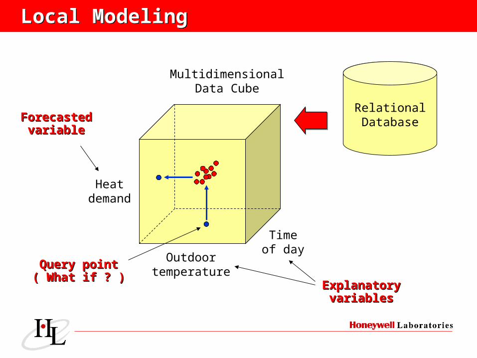
Outdoortemperature
Timeof day
Heatdemand
ForecastedForecastedvariablevariable
ExplanatoryExplanatoryvariablesvariables
Query pointQuery point( What if ? )( What if ? )
RelationalDatabase
MultidimensionalData Cube
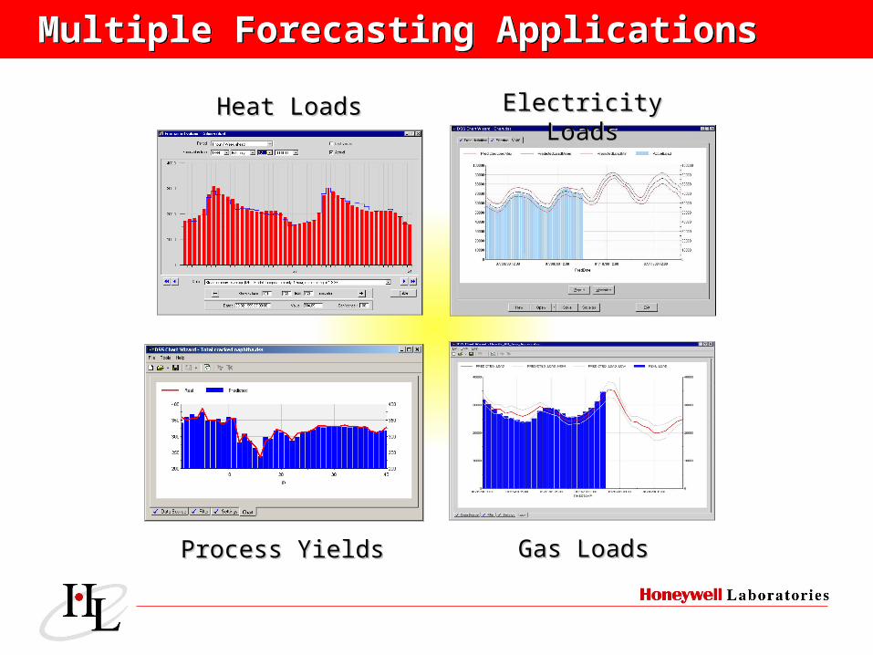
Multiple Forecasting ApplicationsMultiple Forecasting Applications
Heat LoadsHeat Loads
Process YieldsProcess Yields Gas LoadsGas Loads
Electricity LoadsElectricity Loads
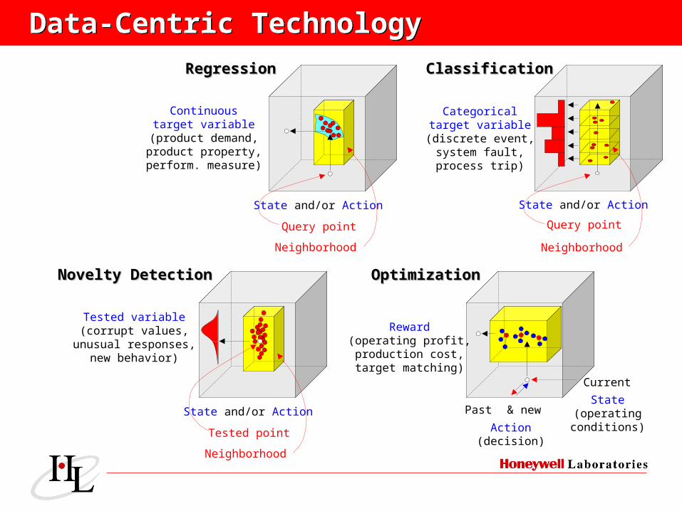
Data-Centric TechnologyData-Centric Technology
Continuoustarget variable
(product demand,product property,perform. measure)
State and/or Action
Neighborhood
Query point
Categoricaltarget variable(discrete event,
system fault,process trip)
State and/or Action
Neighborhood
Query point
Action(decision)
State(operatingconditions)
Reward(operating profit,production cost,target matching)
& new
Current
Past
Novelty DetectionNovelty Detection OptimizationOptimization
RegressionRegression ClassificationClassification
Tested variable(corrupt values,
unusual responses,new behavior)
State and/or Action
Neighborhood
Tested point
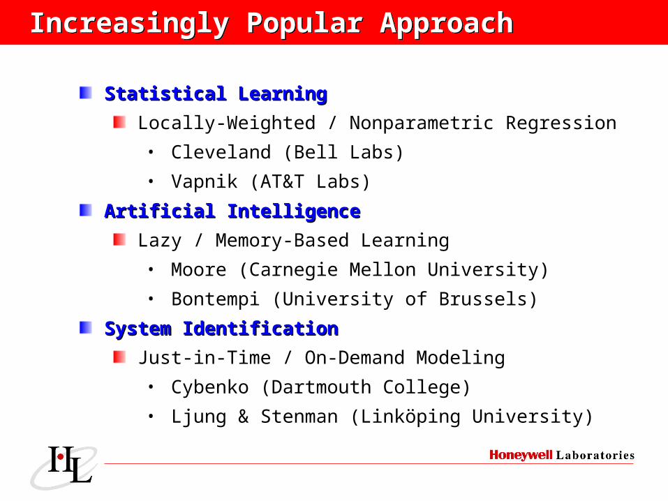
Increasingly Popular ApproachIncreasingly Popular Approach
Statistical LearningStatistical Learning
Locally-Weighted / Nonparametric Regression
• Cleveland (Bell Labs)
• Vapnik (AT&T Labs)
Artificial IntelligenceArtificial Intelligence
Lazy / Memory-Based Learning
• Moore (Carnegie Mellon University)
• Bontempi (University of Brussels)
System IdentificationSystem Identification
Just-in-Time / On-Demand Modeling
• Cybenko (Dartmouth College)
• Ljung & Stenman (Linköping University)
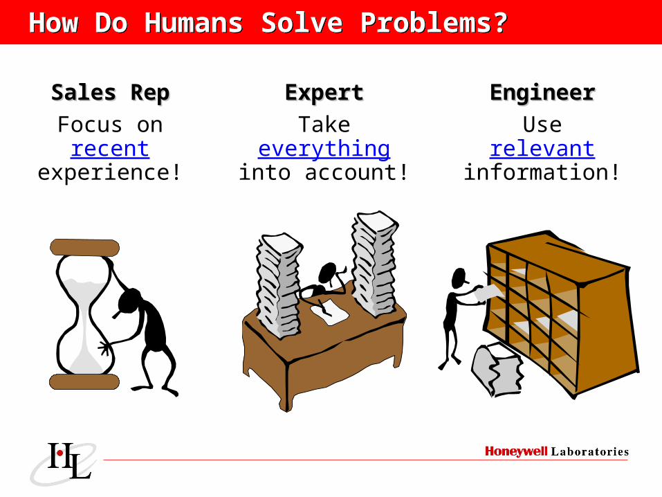
How Do Humans Solve Problems?How Do Humans Solve Problems?
ExpertExpert
Takeeverything
into account!
Sales RepSales Rep
Focus onrecent
experience!
EngineerEngineer
Userelevant
information!
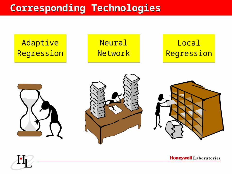
Corresponding TechnologiesCorresponding Technologies
AdaptiveRegressionAdaptive
RegressionLocal
RegressionLocal
RegressionNeural
NetworkNeural
Network
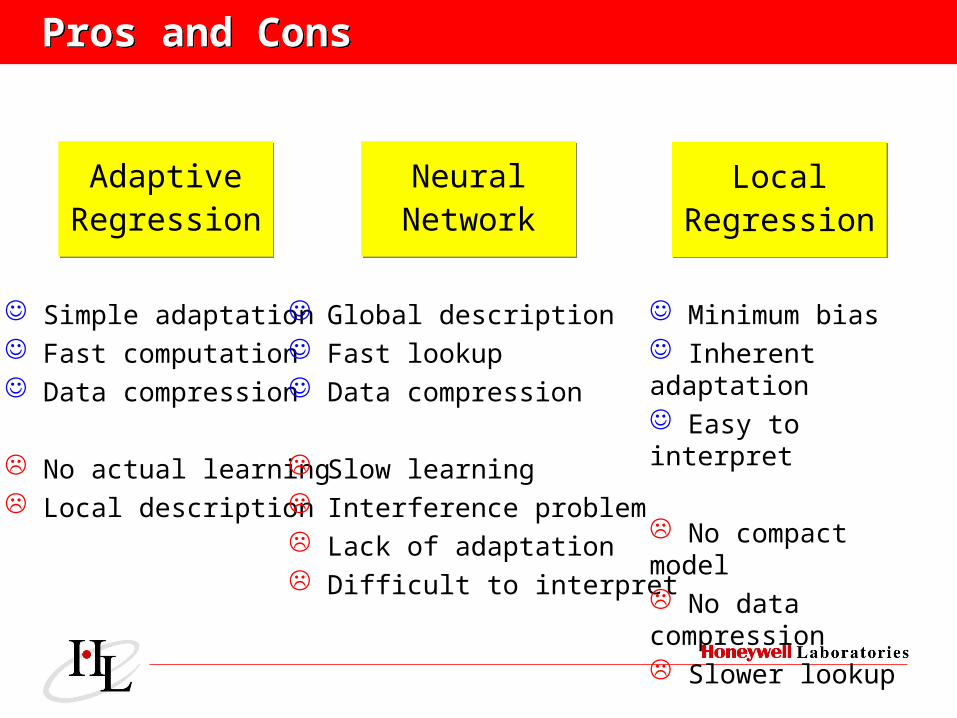
Pros and ConsPros and Cons
Simple adaptation Fast computation Data compression
No actual learning Local description
Global description Fast lookup Data compression
Slow learning Interference problem Lack of adaptation Difficult to interpret
Minimum bias Inherent adaptation Easy to interpret
No compact model No data compression Slower lookup
AdaptiveRegressionAdaptive
RegressionLocal
RegressionLocal
RegressionNeural
NetworkNeural
Network
Addressing DimensionalityAddressing Dimensionality
No Locality in High Dimension?No Locality in High Dimension?
Addressing DimensionalityAddressing Dimensionality
No Locality in High Dimension?No Locality in High Dimension?
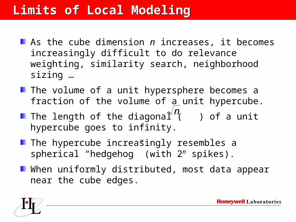
Limits of Local ModelingLimits of Local Modeling
As the cube dimension n increases, it becomes increasingly difficult to do relevance weighting, similarity search, neighborhood sizing …
The volume of a unit hypersphere becomes a fraction of the volume of a unit hypercube.
The length of the diagonal ( ) of a unit hypercube goes to infinity.
The hypercube increasingly resembles a spherical “hedgehog” (with 2n spikes).
When uniformly distributed, most data appear near the cube edges.
n
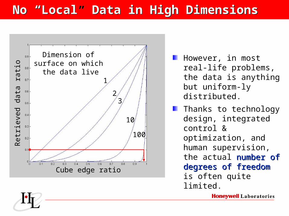
No “Local” Data in High DimensionsNo “Local” Data in High Dimensions
1
23
10
100
Cube edge ratio
Retr
ieved
data
rati
o
Dimension of surface on which
the data live
However, in most real-life problems, the data is anything but uniform-ly distributed.
Thanks to technology design, integrated control & optimization, and human supervision, the actual number of number of degrees of freedomdegrees of freedom is often quite limited.
Local Modeling RevisitedLocal Modeling Revisited
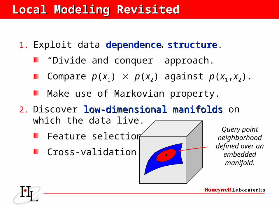
1. Exploit data dependence structuredependence structure.
“Divide and conquer” approach.
Compare p(x1) p(x2) against p(x1,x2).
Make use of Markovian property.
2. Discover low-dimensional manifoldslow-dimensional manifolds on which the data live.
Feature selection.
Cross-validation.
Query point neighborhood
defined over an embedded manifold.
Local Modeling RevisitedLocal Modeling Revisited
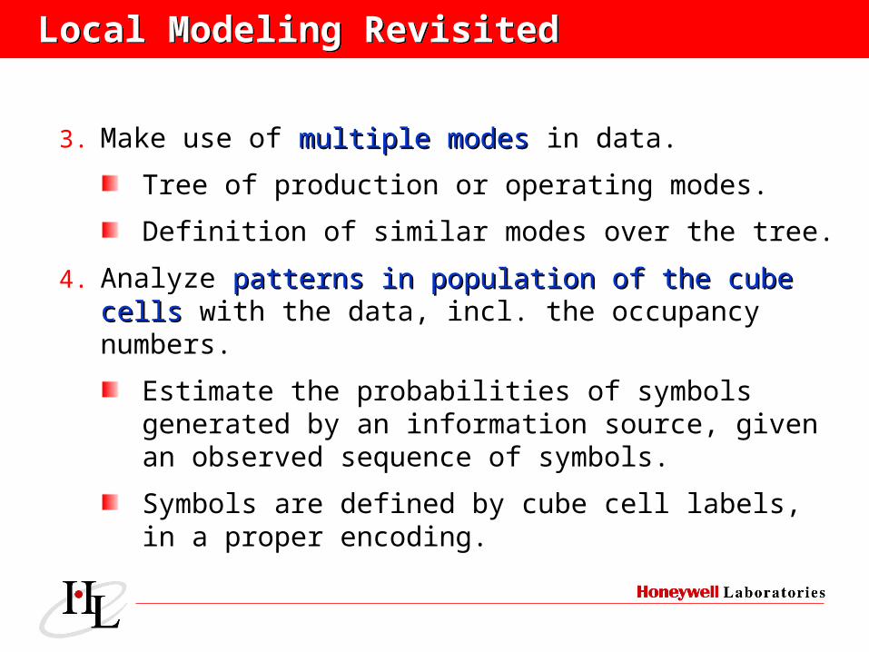
3. Make use of multiple modesmultiple modes in data.
Tree of production or operating modes.
Definition of similar modes over the tree.
4. Analyze patterns in population of the cube cellspatterns in population of the cube cells with the data, incl. the occupancy numbers.
Estimate the probabilities of symbols generated by an information source, given an observed sequence of symbols.
Symbols are defined by cube cell labels, in a proper encoding.
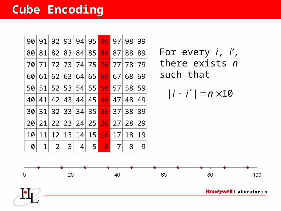
Cube EncodingCube Encoding
90 91 92 93 94 95 96 97 98 99
80 81 82 83 84 85 86 87 88 89
70 71 72 73 74 75 76 77 78 79
60 61 62 63 64 65 66 67 68 69
50 51 52 53 54 55 56 57 58 59
40 41 42 43 44 45 46 47 48 49
30 31 32 33 34 35 36 37 38 39
20 21 22 23 24 25 26 27 28 29
10 11 12 13 14 15 16 17 18 19
0 1 2 3 4 5 6 7 8 9
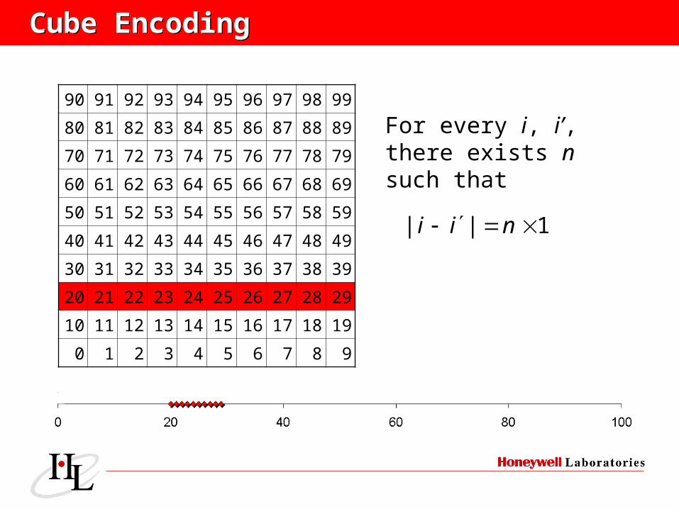
1|| nii
For every i, i’, there exists nsuch that
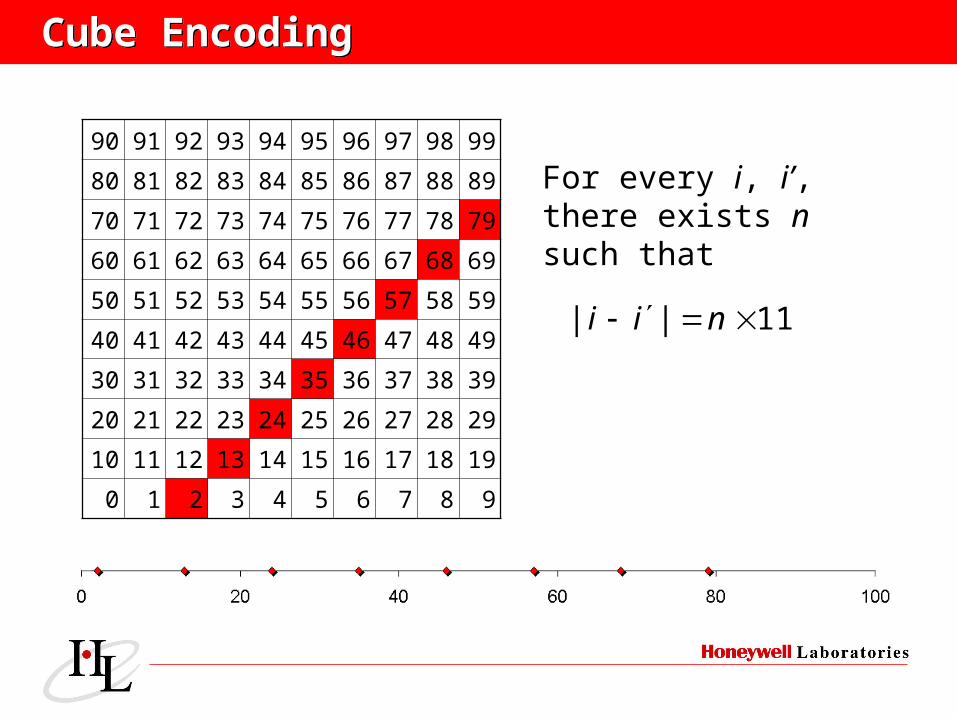
Cube EncodingCube Encoding
90 91 92 93 94 95 96 97 98 99
80 81 82 83 84 85 86 87 88 89
70 71 72 73 74 75 76 77 78 79
60 61 62 63 64 65 66 67 68 69
50 51 52 53 54 55 56 57 58 59
40 41 42 43 44 45 46 47 48 49
30 31 32 33 34 35 36 37 38 39
20 21 22 23 24 25 26 27 28 29
10 11 12 13 14 15 16 17 18 19
0 1 2 3 4 5 6 7 8 9
10|| nii
For every i, i’, there exists nsuch that
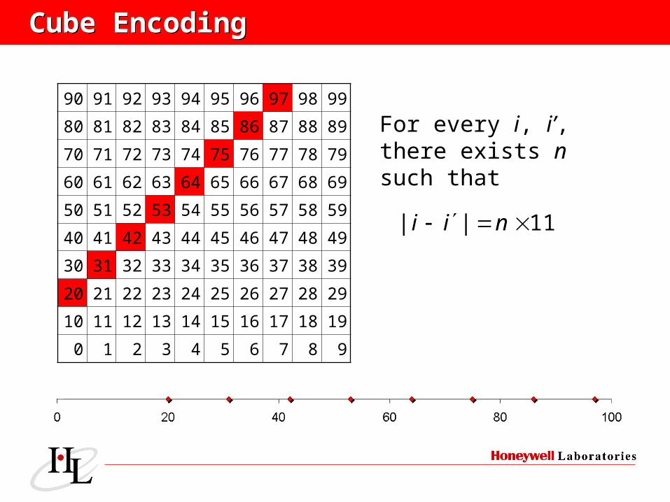
Cube EncodingCube Encoding
90 91 92 93 94 95 96 97 98 99
80 81 82 83 84 85 86 87 88 89
70 71 72 73 74 75 76 77 78 79
60 61 62 63 64 65 66 67 68 69
50 51 52 53 54 55 56 57 58 59
40 41 42 43 44 45 46 47 48 49
30 31 32 33 34 35 36 37 38 39
20 21 22 23 24 25 26 27 28 29
10 11 12 13 14 15 16 17 18 19
0 1 2 3 4 5 6 7 8 9
11|| nii
For every i, i’, there exists nsuch that
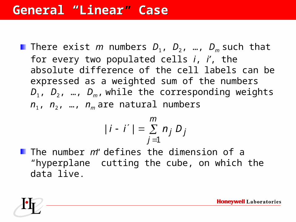
General “Linear” CaseGeneral “Linear” Case
There exist m numbers D1, D2, …, Dm such that for every two populated cells i, i’, the absolute difference of the cell labels can be expressed as a weighted sum of the numbers D1, D2, …, Dm, while the corresponding weights n1, n2, …, nm are natural numbers
The number m defines the dimension of a “hyperplane” cutting the cube, on which the data live.
m
jjj Dnii
1||
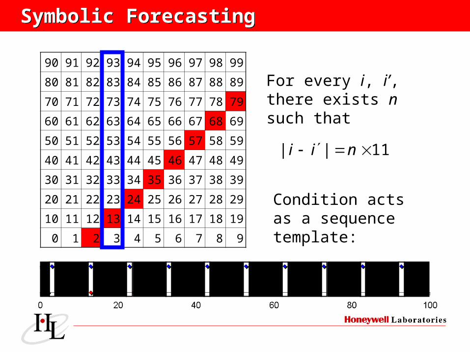
Symbolic ForecastingSymbolic Forecasting
90 91 92 93 94 95 96 97 98 99
80 81 82 83 84 85 86 87 88 89
70 71 72 73 74 75 76 77 78 79
60 61 62 63 64 65 66 67 68 69
50 51 52 53 54 55 56 57 58 59
40 41 42 43 44 45 46 47 48 49
30 31 32 33 34 35 36 37 38 39
20 21 22 23 24 25 26 27 28 29
10 11 12 13 14 15 16 17 18 19
0 1 2 3 4 5 6 7 8 9
11|| nii
For every i, i’, there exists nsuch that
Condition actsas a sequencetemplate:
Symbolic ForecastingSymbolic Forecasting
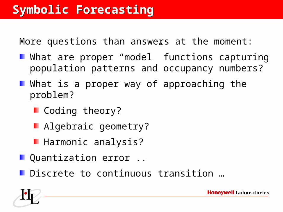
More questions than answers at the moment:
What are proper “model” functions capturing population patterns and occupancy numbers?
What is a proper way of approaching the problem?
Coding theory?
Algebraic geometry?
Harmonic analysis?
Quantization error ..
Discrete to continuous transition …

Decision-Making ProcessDecision-Making Process
Lessons LearntLessons Learnt
Decision-Making ProcessDecision-Making Process
Lessons LearntLessons Learnt

Hypothesis Formulation …Hypothesis Formulation …
Two of world’s leading economists present quiteTwo of world’s leading economists present quitedistinct views of globalization in their new books:distinct views of globalization in their new books:
Joseph Stiglitz
Globalization and Its Discontents
Jagdish Bhagwati
In Defense of Globalization

Feature Selection …Feature Selection …
The Wall Street Journal Europe, Dec 2, 2002The Wall Street Journal Europe, Dec 2, 2002The Globalization Stirs Debate at U.S. UniversitiesThe Globalization Stirs Debate at U.S. Universities::
In Latin America, Mr. StiglitzMr. Stiglitz says, growth in the 1990s was slower, at 2.9% a year, than it was during the days of trade protectionism in the 1960s, when the region’s annual growth rate was about 5.4%.
Mr. BhagwatiMr. Bhagwati argues … that women’s wages in many developing countries has increased as multinational investment has risen.

Training Data Selection …Training Data Selection …
The Wall Street Journal Europe, Dec 2, 2002The Wall Street Journal Europe, Dec 2, 2002The Globalization Stirs Debate at U.S. UniversitiesThe Globalization Stirs Debate at U.S. Universities::
Mr. StiglitzMr. Stiglitz cites a World Bank study showing that the number of people living on less than $2 a day increasedincreased by nearly 100 million during the booming 1990s1990s.
Mr. BhagwatiMr. Bhagwati argues that the number of people living on less than $2 a day declined by nearly 500 million between 1976 and 1998between 1976 and 1998.
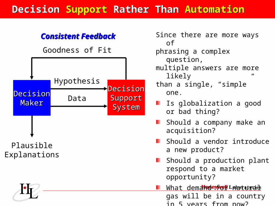
Decision Support Rather Than AutomationDecision Support Rather Than Automation
DecisionDecisionMakerMaker
DecisionDecisionMakerMaker
DecisionDecisionSupportSupportSystemSystem
DecisionDecisionSupportSupportSystemSystem
Hypothesis
Data
Goodness of Fit
PlausibleExplanations
Since there are more ways ofphrasing a complex question,multiple answers are more likelythan a single, “simple” one.
Is globalization a good or bad thing?
Should a company make an acquisition?
Should a vendor introduce a new product?
Should a production plant respond to a market opportunity?
What demand for natural gas will be in a country in 5 years from now?
Consistent FeedbackConsistent Feedback
Humans To Stay in ControlHumans To Stay in Control
At the moment, computerized data analysis is more likely to be delivered as decision supportdecision support rather than closed-loop control.
Success depends to a large extent on effective effective interactioninteraction between humans and computers.
For the foreseeable future, formulation of formulation of hypotheseshypotheses and interpretation of resultsinterpretation of results is likely to stay with the people.
Commercial decision support software should support a typical usage scenariotypical usage scenario.