Hindawi Publishing CorporationEURASIP Journal on Advances in Signal ProcessingVolume 2009, Article ID 298605, 10 pagesdoi:10.1155/2009/298605

Research Article

Database of Multichannel In-Ear and Behind-the-EarHead-Related and Binaural Room Impulse Responses

H. Kayser, S. D. Ewert, J. Anemuller, T. Rohdenburg, V. Hohmann, and B. Kollmeier

Medizinische Physik, Universitat Oldenburg, 26111 Oldenburg, Germany

Correspondence should be addressed to H. Kayser, hendrik.kayser@uni-oldenburg.de

Received 15 December 2008; Accepted 4 June 2009

Recommended by Hugo Fastl

An eight-channel database of head-related impulse responses (HRIRs) and binaural room impulse responses (BRIRs) isintroduced. The impulse responses (IRs) were measured with three-channel behind-the-ear (BTEs) hearing aids and an in-earmicrophone at both ears of a human head and torso simulator. The database aims at providing a tool for the evaluation ofmultichannel hearing aid algorithms in hearing aid research. In addition to the HRIRs derived from measurements in an anechoicchamber, sets of BRIRs for multiple, realistic head and sound-source positions in four natural environments reflecting daily-life communication situations with different reverberation times are provided. For comparison, analytically derived IRs for arigid acoustic sphere were computed at the multichannel microphone positions of the BTEs and differences to real HRIRs wereexamined. The scenes’ natural acoustic background was also recorded in each of the real-world environments for all eight channels.Overall, the present database allows for a realistic construction of simulated sound fields for hearing instrument research and,consequently, for a realistic evaluation of hearing instrument algorithms.

Copyright © 2009 H. Kayser et al. This is an open access article distributed under the Creative Commons Attribution License,which permits unrestricted use, distribution, and reproduction in any medium, provided the original work is properly cited.

1. Introduction

Performance evaluation is an important part of hearinginstrument algorithm research since only a careful evaluationof accomplished effects can identify truly promising andsuccessful signal enhancement methods. The gold standardfor evaluation will always be the unconstrained real-worldenvironment, which comes however at a relatively high costin terms of time and effort for performance comparisons.

Simulation approaches to the evaluation task are thefirst steps in identifying good signal processing algorithms.It is therefore important to utilize simulated input signalsthat represent real-world signals as faithfully as possible,especially if multimicrophone arrays and binaural hearinginstrument algorithms are considered that expect input fromboth sides of a listener’s head. The simplest approach tomodel the input signals to a multichannel or binaural hearinginstrument is the free-field model. More elaborate modelsare based on analytical formulations of the effect that a rigidsphere has on the acoustic field [1, 2].

Finally, the synthetic generation of multichannel inputsignals by means of convolving recorded (single-channel)

sound signals with impulse responses (IRs) correspondingto the respective spatial sound source positions, and alsodepending on the spatial microphone locations, represents agood approximation to the expected recordings from a real-world sound field. It comes at a fraction of the cost and withvirtually unlimited flexibility in arranging different acousticobjects at various locations in virtual acoustic space if theappropriate room-, head-, and microphone-related impulseresponses are available.

In addition, when recordings from multichannel hearingaids and in-ear microphones in a real acoustic backgroundsound field are available, even more realistic situations can beproduced by superimposing convolved contributions fromlocalized sound sources with the approximately omnidirec-tional real sound field recording at a predefined mixing ratio.By this means, the level of disturbing background noisecan be controlled independently from the localized soundsources.

Under the assumption of a linear and time-invariantpropagation of sound from a fixed source to a receiver,the impulse response completely describes the system. Alltransmission characteristics of the environment and objects

2 EURASIP Journal on Advances in Signal Processing

in the surrounding area are included. The transmission ofsound from a source to human ears is also described inthis way. Under anechoic conditions the impulse responsecontains only the influence of the human head (and torso)and therefore is referred to as head-related impulse response(HRIR). Its Fourier transform is correspondingly referredto as head-related transfer function (HRTF). Binaural head-related IRs recorded in rooms are typically referred to asbinaural room impulse responses (BRIRs).

There are several existing free available databases con-taining HRIRs or HRTFs measured on individual subjectsand different artificial head-and-torso simulators (HATS)[3–6]. However these databases are not suitable to simulatesound impinging on hearing aids located behind the ears(BTEs) as they are limited to two-channel informationrecorded near the entrance of the ear canal. Additionally thedatabases do not reflect the influence of the room acoustics.

For the evaluation of modern hearing aids, whichtypically process 2 or 3 microphone signals per ear, multi-channel input data are required corresponding to the realmicrophone locations (in the case of BTE devices behind theear and outside the pinna) and characterizing the respectiveroom acoustics.

The database presented here therefore improves overexisting publicly available data in two respects: In contrast toother HRIR and BRIR databases, it provides a dummy-headrecording as well as an appropriate number of microphonechannel locations at realistic spatial positions behind the ear.In addition, several room acoustical conditions are included.

Especially for the application in hearing aids, a broad setof test situations is important for developing and testing ofalgorithms performing audio processing. The availability ofmultichannel measurements of HRIRs and BRIRs capturedby hearing aids enables the use of signal processing tech-niques which benefit from multichannel input, for example,blind source separation, sound source localization andbeamforming. Real-world problems, such as head shadingand microphone mismatch [7] can be considered by thismeans.

A comparison between the HRTFs derived from therecorded HRIRs at the in-ear and behind-the-ear positionsand respective modeled HRTFs based on a rigid sphericalhead is presented to analyze deviations between simulationsand a real measurements. Particularly at high frequencies,deviations are expected related to the geometric differencesbetween the real head including the pinnae and the model’sspherical head.

The new database of head-, room- and microphone-related impulse responses, for convenience consistentlyreferred to as HRIRs in the following, contains six-channelhearing aid measurements (three per side) and additionallythe in-ear HRIRs measured on a Bruel & Kjær HATS [8] indifferent environments.

After a short overview of the measurement method andsetup, the acoustic situations contained in the database aresummarized, followed by a description of the analyticalhead model and the methods used to analyze the data.Finally, the results obtained under anechoic conditions arecompared to synthetically generated HRTFs based on the

7.3

7.6

13.6

2.1

2.6

32.7

4

4

4

345

5

5

6

6

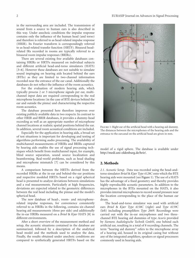
Figure 1: Right ear of the artificial head with a hearing aid dummy.The distances between the microphones of the hearing aids and theentrance to the earcanal on the artificial head are given in mm.

model of a rigid sphere. The database is available underhttp://medi.uni-oldenburg.de/hrir/.

2. Methods

2.1. Acoustic Setup. Data was recorded using the head-and-torso simulator Bruel & Kjær Type 4128C onto which the BTEhearing aids were mounted (see Figure 1). The use of a HATShas the advantage of a fixed geometry and thereby provideshighly reproducible acoustic parameters. In addition to themicrophones in the BTEs mounted on the HATS, it alsoprovides internal microphones to record sound pressure nearthe location corresponding to the place of the human eardrum.

The head-and-torso simulator was used with artificialears Bruel & Kjær Type 4158C (right) and Type 4159C(left) including preamplifiers Type 2669. Recordings werecarried out with the in-ear microphones and two three-channel BTE hearing aid dummies of type Acuris providedby Siemens Audiologische Technik GmbH, one behind eachartificial ear, resulting in a total of 8 recording channels. Theterm “hearing aid dummy” refers to the microphone arrayof a hearing aid, housed in its original casing but withoutany of the integrated amplifiers, speakers or signal processorscommonly used in hearing aids.

EURASIP Journal on Advances in Signal Processing 3

The recorded analog signals were preamplifiedusing a G.R.A.S. Power Module Type 12AA, with theamplification set to +20 dB (in-ear microphones) and aSiemens custom-made pre-amplifier, with an amplificationof +26 dB on the hearing aid microphones. Signalswere converted using a 24-bit multichannel AD/DA-converter (RME Hammerfall DSP Multiface) connectedto a laptop (DELL Latitude 610D, Pentium M processor@1.73Ghz,1GB RAM) via a PCMCIA-card and the digitaldata was stored either on the internal or an externalhard disk. The software used for the recordings wasMATLAB (MathWorks, Versions 7.1/7.2, R14/R2006a) witha professional tool for multichannel I/O and real-timeprocessing of audio signals (SoundMex2 [9]).

The measurement stimuli for measuring a HRIR weregenerated digitally on the computer using MATLAB-scripts (developed in-house) and presented via the AD/DA-converter to a loudspeaker. The measurement stimuli wereemitted by an active 2-channel coaxial broadband loud-speaker (Tannoy 800A LH). All data was recorded at asampling rate of 48 kHz and stored at a resolution of 32 Bit.

2.2. HRIR Measurement. The HRIR measurements werecarried out for a variety of natural recording situations.Some of the scenarios were suffering from relatively highlevels of ambient noise during the recording. Additionally,at some recording sites, special care had to be taken ofthe public (e.g., cafeteria). The measurement procedurewas therefore required to be of low annoyance while themeasurement stimuli had to be played back at a sufficientlevel and duration to satisfy the demand of a high signal-to-noise ratio imposed by the use of the recorded HRIRsfor development and high-quality auralization purposes.To meet all requirements, the recently developed modifiedinverse-repeated sequence (MIRS) method [10] was used.The method is based on maximum length sequences (MLS)which are highly robust against transient noise since theirenergy is distributed uniformly in the form of noise over thewhole impulse response [11]. Furthermore, the broadbandnoise characteristics of MLS stimuli made them suitablefor presentation in the public rather than, for example,sine-sweep stimuli-based methods [12]. However, MLSs areknown to be relatively sensitive to (even weak) nonlinearitiesin the measurement setup. Since the recordings at public sitesrequired partially high levels reproduced by small scale andportable equipment, the risk of non-linear distortions waspresent. Inverse repeated sequences (IRS) are a modificationto MLSs which show high robustness against even-ordernonlinear distortions [13]. An IRS consists of two concate-nated MLS s(n) and its inverse:

IRS(n) =⎧⎨

⎩

s(n), n even,

−s(n), n odd,0 ≤ n ≤ 2L, (1)

where L is the period of the generating MLS. The IRStherefore has a period of 2L. In the MIRS method employedhere, IRSs of different orders are used in one measurementprocess and the resulting impulse responses of different

lengths are median-filtered to further suppress the effectof uneven-order nonlinear distortions after the followingscheme: A MIRS consists of several successive IRS of differentorders. In the evaluation step, the resulting periodic IRs ofthe same order were averaged yielding a set of IRs of differentorders. The median of these IRs was calculated and the finalIR was shortened to length corresponding to the lowest order.The highest IRS order in the measurements was 19, which isequal to a length of 10.92 seconds at the used sampling rateof 48 kHz. The overall MIRS was 32.77 seconds in durationand the calculated raws IRs were 2.73 seconds correspondingto 131072 samples.

The MIRS method combines the advantages of MLSmeasurements with high immunity against non-linear dis-tortions. A comparison of the measurement results to anefficient method proposed by Farina [12] showed that theMIRS technique achieves competitive results in anechoicconditions with regard to signal-to-noise ratio and was bettersuited in public conditions (for details see [10]).

The transfer characteristics of the measurement systemwas not compensated for in the HRIRs presented here,since it does not effect the interaural and microphonearray differences. The impulse response of the loudspeakermeasured by a probe microphone at the HATS position inthe anechoic chamber is provided as part of the database.

2.3. Content of the Database. A summary of HRIR mea-surements and recordings of ambient acoustic backgrounds(noise) is found in Table 1.

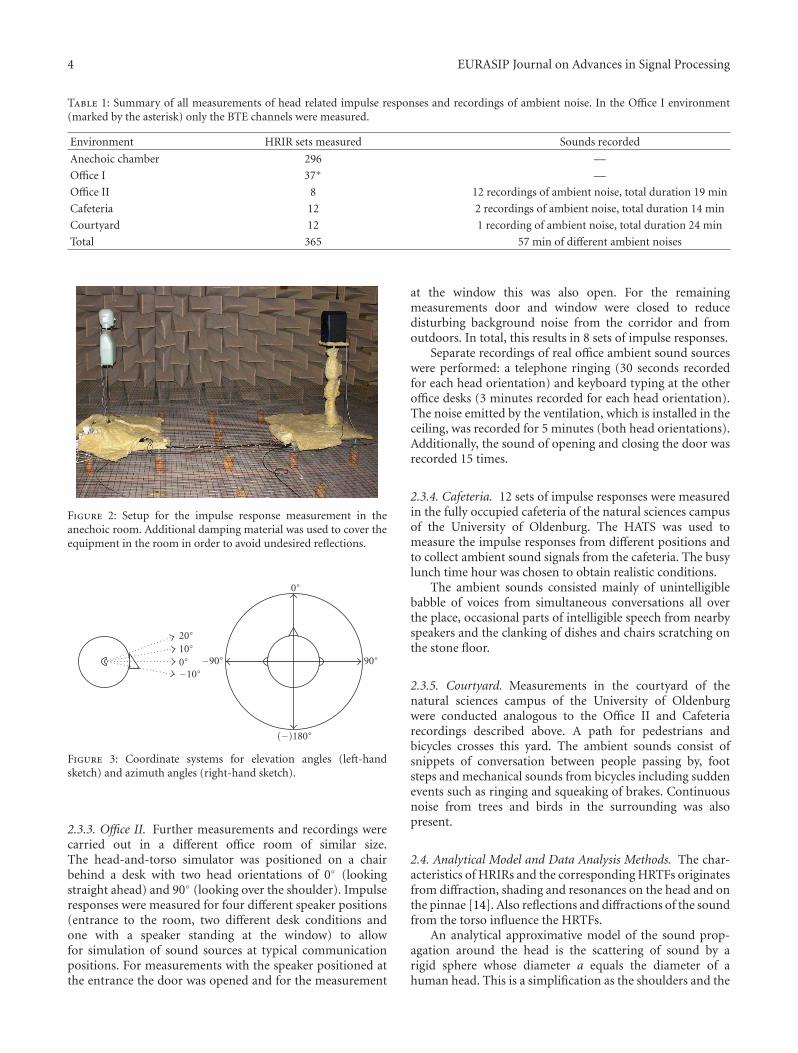
2.3.1. Anechoic Chamber. To simulate a nonreverberantsituation, the measurements were conducted in the anechoicchamber of the University of Oldenburg. The HATS wasfixed on a computer-controlled turntable (Bruel & Kjær Type5960C with Controller Type 5997) and placed opposite to thespeaker in the room as shown in Figure 2. Impulse responseswere measured for distances of 0.8 m and 3 m betweenspeaker and the HATS. The larger distance corresponds toa far-field situation (which is, e.g., commonly required bybeam-forming algorithms) whereas for the smaller distancenear-field effects may occur. For each distance, 4 angles ofelevation were measured ranging from −10◦ to 20◦ in stepsof 10◦. For each elevation the azimuth angle of the source tothe HATS was varied from 0◦ (front) to −180◦ (left turn) insteps of 5◦ (cf. Figure 3). Hence, a total of 296 (= 37×4×2)sets of impulse responses were measured.

2.3.2. Office I. In an office room at the University ofOldenburg similar measurements were conducted, coveringthe systematic variation of the sources’ spatial positions. TheHATS was placed on a desk and the speaker was moved inthe front hemisphere (from −90◦ to +90◦) at a distance of1 m with an elevation angle of 0◦. The step size of alterationof the azimuth angle was 5◦ as for the anechoic chamber.

For this environment only the BTE channels weremeasured.

A detailed sketch of the recording setup for this and theother environments is provided as a part of the database.

4 EURASIP Journal on Advances in Signal Processing

Table 1: Summary of all measurements of head related impulse responses and recordings of ambient noise. In the Office I environment(marked by the asterisk) only the BTE channels were measured.

Environment HRIR sets measured Sounds recorded

Anechoic chamber 296 —

Office I 37∗ —

Office II 8 12 recordings of ambient noise, total duration 19 min

Cafeteria 12 2 recordings of ambient noise, total duration 14 min

Courtyard 12 1 recording of ambient noise, total duration 24 min

Total 365 57 min of different ambient noises

Figure 2: Setup for the impulse response measurement in theanechoic room. Additional damping material was used to cover theequipment in the room in order to avoid undesired reflections.

20◦

10◦

0◦−10◦

0◦

−90◦ 90◦

(−)180◦

Figure 3: Coordinate systems for elevation angles (left-handsketch) and azimuth angles (right-hand sketch).

2.3.3. Office II. Further measurements and recordings werecarried out in a different office room of similar size.The head-and-torso simulator was positioned on a chairbehind a desk with two head orientations of 0◦ (lookingstraight ahead) and 90◦ (looking over the shoulder). Impulseresponses were measured for four different speaker positions(entrance to the room, two different desk conditions andone with a speaker standing at the window) to allowfor simulation of sound sources at typical communicationpositions. For measurements with the speaker positioned atthe entrance the door was opened and for the measurement

at the window this was also open. For the remainingmeasurements door and window were closed to reducedisturbing background noise from the corridor and fromoutdoors. In total, this results in 8 sets of impulse responses.

Separate recordings of real office ambient sound sourceswere performed: a telephone ringing (30 seconds recordedfor each head orientation) and keyboard typing at the otheroffice desks (3 minutes recorded for each head orientation).The noise emitted by the ventilation, which is installed in theceiling, was recorded for 5 minutes (both head orientations).Additionally, the sound of opening and closing the door wasrecorded 15 times.

2.3.4. Cafeteria. 12 sets of impulse responses were measuredin the fully occupied cafeteria of the natural sciences campusof the University of Oldenburg. The HATS was used tomeasure the impulse responses from different positions andto collect ambient sound signals from the cafeteria. The busylunch time hour was chosen to obtain realistic conditions.

The ambient sounds consisted mainly of unintelligiblebabble of voices from simultaneous conversations all overthe place, occasional parts of intelligible speech from nearbyspeakers and the clanking of dishes and chairs scratching onthe stone floor.

2.3.5. Courtyard. Measurements in the courtyard of thenatural sciences campus of the University of Oldenburgwere conducted analogous to the Office II and Cafeteriarecordings described above. A path for pedestrians andbicycles crosses this yard. The ambient sounds consist ofsnippets of conversation between people passing by, footsteps and mechanical sounds from bicycles including suddenevents such as ringing and squeaking of brakes. Continuousnoise from trees and birds in the surrounding was alsopresent.

2.4. Analytical Model and Data Analysis Methods. The char-acteristics of HRIRs and the corresponding HRTFs originatesfrom diffraction, shading and resonances on the head and onthe pinnae [14]. Also reflections and diffractions of the soundfrom the torso influence the HRTFs.

An analytical approximative model of the sound prop-agation around the head is the scattering of sound by arigid sphere whose diameter a equals the diameter of ahuman head. This is a simplification as the shoulders and the

EURASIP Journal on Advances in Signal Processing 5

pinnae are neglected and the head is regarded as sphericallysymmetric.

The solution in the frequency domain for the diffractionof sound waves on a sphere traces back to Lord Rayleigh[15] in 1904. He derived the transfer function H(∞, θ,μ)dependent on the normalized frequency μ = ka = 2π f a/c(c: sound velocity) for an infinitely distant source impingingat the angle θ between the surface normal at the observationpoint and the source:

H(∞, θ,μ

) = 1μ2

∞∑

m=0

(−i)m−1(2m + 1)Pm(cos θ)h′m(μ) , (2)

where Pm denotes the Legendre polynomials, hm the mth-order spherical Hankel function and h′m its derivative.Rabinowitz et al. [16] presented a solution for a point sourcein the distance r from the center of the sphere:

H(r, θ,μ

) = − r

aμe −iμr/aΨ, (3)

with

Ψ =∞∑

m=0

(2m + 1)Pm(cos θ)hm(μr/a

)

h′m(μ) , r > α. (4)

2.4.1. Calculation of Binaural Cues. The binaural cues,namely the interaural level difference (ILD), the interauralphase difference (IPD) and derived therefrom the interauraltime difference (ITD), can be calculated in the frequencydomain from a measured or simulated HRTF [17]. IfHl(α,ϕ, f ) denotes the HRTF from the source to the leftear and Hr(α,ϕ, f ) the transmission to the right ear, theinteraural transfer function (ITF) is given by

ITF(α,ϕ, f

) = Hl(α,ϕ, f

)

Hr(α,ϕ, f

) , (5)

with α and ϕ the azimuth and elevations angles, respectively,as shown in Figure 3 and f representing the frequency in Hz.

The ILD is determined by

ILD(α,ϕ, f

) = 20 · log10

(∣∣ITF

(α,ϕ, f

)∣∣). (6)

The IPD can also be calculated from the ITF. Derivation withrespect to the frequency f yields the ITD which equals thegroup delay between both ears:

IPD(α,ϕ, f

) = arg(ITF

(α,ϕ, f

)),

ITD(α,ϕ, f

) = − 12π

d

dfIPD

(α,ϕ, f

).

(7)

Kuhn presented the limiting cases for (2) in [2]. For lowfrequencies corresponding to the case ka � 1 the transferfunction of the spherical head model simplifies to

Hl f(∞, θ,μ

) ≈ 1− i32μ cos θ. (8)

This yields an angle of incidence independent ILD of 0 dBand an angle dependent IPD. In the coordinate system givenin Figure 3 the IPD amounts to

IPDl f (α) ≈ 3ka sinα, (9)

which results in

ITDl f (α) ≈ 6πac

sinα. (10)

For high frequencies the propagation of the waves isdescribed as “creeping waves” traveling around the spherewith approximately the speed of sound. In this case, the ITDcan be derived from geometric treatment by the differencebetween the distance from the source to the left ear and theright ear considering the path along the surface of the sphere[18]:

ITDh f ≈ 2πac

(sin(α) + α). (11)

With the approximation α ≈ sinα, (tolerating an error of5.5% for α = 135◦ and an error of 11% for α = 150◦ [2]) (11)yields:

ITDh f (α) ≈ 4πac

sinα, (12)

which equals 2/3 times the result of (10).In practice, the measured IPD is contaminated by noise.

Hence, the data was preprocessed before the ITD wasdetermined. First, the amplitude of the ITF was equalized tounity by calculating the sign of the complex valued ITF:

ITF(α,ϕ, f

) = sign(ITF

(α,ϕ, f

))

= ITF(α,ϕ, f

)

∣∣ITF

(α,ϕ, f

)∣∣ .

(13)

The result was then smoothed applying a sliding averagewith a 20-samples window. The ITD was obtained for aspecific frequency by calculating the weighted mean of theITD (derived from the smoothed IPD) for a chosen rangearound this frequency. As weighting function the coherencefunction γ was used, respectively a measure for the coherenceγn which is obtained from

γn =∣∣∣ITF(α,ϕ, f )

∣∣∣n

︸ ︷︷ ︸

smoothed

. (14)

The function was raised to the power of n to control thestrength of suppression of data with a weak coherence. In theanalysis n = 6 turned out to be a suitable choice.

3. Results

3.1. Quality of the Measurements. As evaluation of thequality, the signal-to-noise ratio (SNR) of the measuredimpulse responses was calculated for each environment. Theaverage noise power was estimated from the noise floor

6 EURASIP Journal on Advances in Signal Processing

irnoise(t) for the interval Tend at end of the measured IR,where the IR has declined below the noise level. The durationof the measured IRs was sufficient to assume that only noisewas present in this part of the measured IR. With the averagepower estimated for the entire duration T = 2.73 s of themeasured IR, ir(t), the SNR was calculated as

SNR = 10 log10

⟨ir2(t)

⟩

T⟨

ir2noise(t)

⟩

Tend

, (15)

where 〈·〉 denotes the temporal average.The results are given in Table 2.

3.2. Reverberation Time of the Different Environments. Thereverberation time T60 denotes the time that it takes for thesignal energy to decay by 60 dB after the playback of thesignal is stopped. It was estimated from a room impulseresponse of duration T employing the method of Schroederintegration [19]. In the Schroeder integration, the energydecay curve (EDC) is obtained by reverse-time integrationof the squared impulse response:

EDC (t) = 10 log10

∫ Tt ir

2(τ)dτ∫ T

0 ir2(τ)dτ. (16)

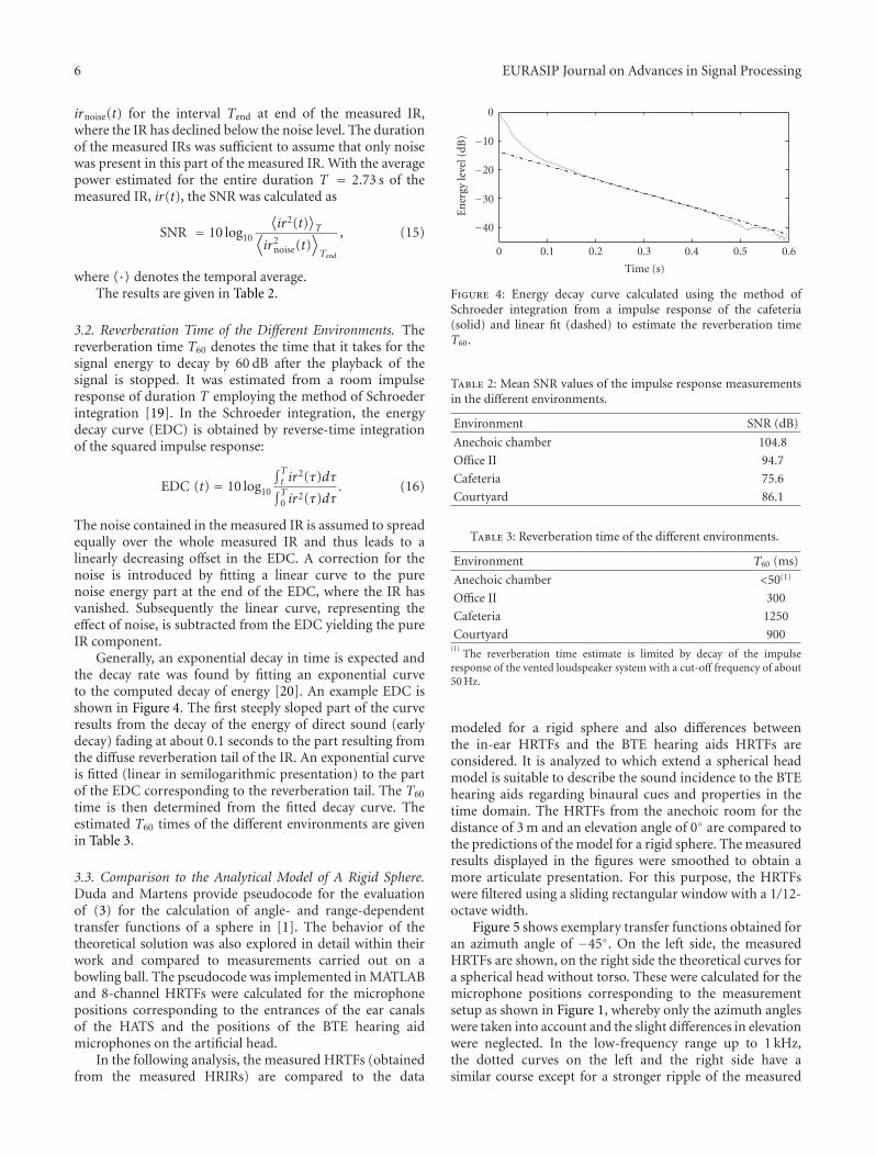
The noise contained in the measured IR is assumed to spreadequally over the whole measured IR and thus leads to alinearly decreasing offset in the EDC. A correction for thenoise is introduced by fitting a linear curve to the purenoise energy part at the end of the EDC, where the IR hasvanished. Subsequently the linear curve, representing theeffect of noise, is subtracted from the EDC yielding the pureIR component.

Generally, an exponential decay in time is expected andthe decay rate was found by fitting an exponential curveto the computed decay of energy [20]. An example EDC isshown in Figure 4. The first steeply sloped part of the curveresults from the decay of the energy of direct sound (earlydecay) fading at about 0.1 seconds to the part resulting fromthe diffuse reverberation tail of the IR. An exponential curveis fitted (linear in semilogarithmic presentation) to the partof the EDC corresponding to the reverberation tail. The T60

time is then determined from the fitted decay curve. Theestimated T60 times of the different environments are givenin Table 3.

3.3. Comparison to the Analytical Model of A Rigid Sphere.Duda and Martens provide pseudocode for the evaluationof (3) for the calculation of angle- and range-dependenttransfer functions of a sphere in [1]. The behavior of thetheoretical solution was also explored in detail within theirwork and compared to measurements carried out on abowling ball. The pseudocode was implemented in MATLABand 8-channel HRTFs were calculated for the microphonepositions corresponding to the entrances of the ear canalsof the HATS and the positions of the BTE hearing aidmicrophones on the artificial head.

In the following analysis, the measured HRTFs (obtainedfrom the measured HRIRs) are compared to the data

−40

−30

−20

−10

0

En

ergy

leve

l(dB

)

0 0.1 0.2 0.3 0.4 0.5 0.6

Time (s)

Figure 4: Energy decay curve calculated using the method ofSchroeder integration from a impulse response of the cafeteria(solid) and linear fit (dashed) to estimate the reverberation timeT60.

Table 2: Mean SNR values of the impulse response measurementsin the different environments.

Environment SNR (dB)

Anechoic chamber 104.8

Office II 94.7

Cafeteria 75.6

Courtyard 86.1

Table 3: Reverberation time of the different environments.

Environment T60 (ms)

Anechoic chamber <50(1)

Office II 300

Cafeteria 1250

Courtyard 900(1)

The reverberation time estimate is limited by decay of the impulseresponse of the vented loudspeaker system with a cut-off frequency of about50 Hz.

modeled for a rigid sphere and also differences betweenthe in-ear HRTFs and the BTE hearing aids HRTFs areconsidered. It is analyzed to which extend a spherical headmodel is suitable to describe the sound incidence to the BTEhearing aids regarding binaural cues and properties in thetime domain. The HRTFs from the anechoic room for thedistance of 3 m and an elevation angle of 0◦ are compared tothe predictions of the model for a rigid sphere. The measuredresults displayed in the figures were smoothed to obtain amore articulate presentation. For this purpose, the HRTFswere filtered using a sliding rectangular window with a 1/12-octave width.

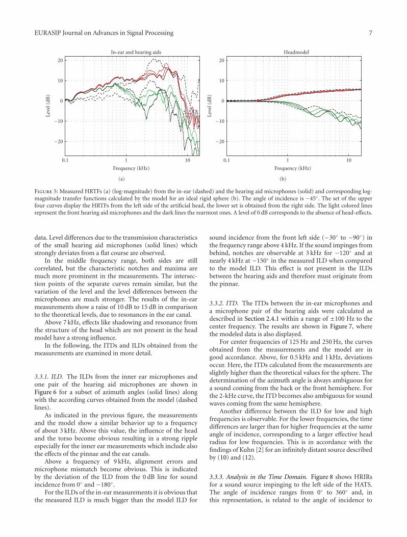
Figure 5 shows exemplary transfer functions obtained foran azimuth angle of −45◦. On the left side, the measuredHRTFs are shown, on the right side the theoretical curves fora spherical head without torso. These were calculated for themicrophone positions corresponding to the measurementsetup as shown in Figure 1, whereby only the azimuth angleswere taken into account and the slight differences in elevationwere neglected. In the low-frequency range up to 1 kHz,the dotted curves on the left and the right side have asimilar course except for a stronger ripple of the measured

EURASIP Journal on Advances in Signal Processing 7

−20

−10

0

10

20

Leve

l(dB

)

0.1 1 10

Frequency (kHz)

In-ear and hearing aids

(a)

−20

−10

0

10

20

Leve

l(dB

)

0.1 1 10

Frequency (kHz)

Headmodel

(b)

Figure 5: Measured HRTFs (a) (log-magnitude) from the in-ear (dashed) and the hearing aid microphones (solid) and corresponding log-magnitude transfer functions calculated by the model for an ideal rigid sphere (b). The angle of incidence is −45◦. The set of the upperfour curves display the HRTFs from the left side of the artificial head, the lower set is obtained from the right side. The light colored linesrepresent the front hearing aid microphones and the dark lines the rearmost ones. A level of 0 dB corresponds to the absence of head-effects.

data. Level differences due to the transmission characteristicsof the small hearing aid microphones (solid lines) whichstrongly deviates from a flat course are observed.

In the middle frequency range, both sides are stillcorrelated, but the characteristic notches and maxima aremuch more prominent in the measurements. The intersec-tion points of the separate curves remain similar, but thevariation of the level and the level differences between themicrophones are much stronger. The results of the in-earmeasurements show a raise of 10 dB to 15 dB in comparisonto the theoretical levels, due to resonances in the ear canal.

Above 7 kHz, effects like shadowing and resonance fromthe structure of the head which are not present in the headmodel have a strong influence.

In the following, the ITDs and ILDs obtained from themeasurements are examined in more detail.

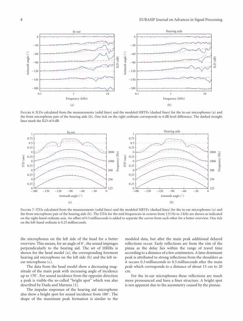
3.3.1. ILD. The ILDs from the inner ear microphones andone pair of the hearing aid microphones are shown inFigure 6 for a subset of azimuth angles (solid lines) alongwith the according curves obtained from the model (dashedlines).

As indicated in the previous figure, the measurementsand the model show a similar behavior up to a frequencyof about 3 kHz. Above this value, the influence of the headand the torso become obvious resulting in a strong rippleespecially for the inner ear measurements which include alsothe effects of the pinnae and the ear canals.

Above a frequency of 9 kHz, alignment errors andmicrophone mismatch become obvious. This is indicatedby the deviation of the ILD from the 0 dB line for soundincidence from 0◦ and −180◦.

For the ILDs of the in-ear measurements it is obvious thatthe measured ILD is much bigger than the model ILD for

sound incidence from the front left side (−30◦ to −90◦) inthe frequency range above 4 kHz. If the sound impinges frombehind, notches are observable at 3 kHz for −120◦ and atnearly 4 kHz at −150◦ in the measured ILD when comparedto the model ILD. This effect is not present in the ILDsbetween the hearing aids and therefore must originate fromthe pinnae.

3.3.2. ITD. The ITDs between the in-ear microphones anda microphone pair of the hearing aids were calculated asdescribed in Section 2.4.1 within a range of ±100 Hz to thecenter frequency. The results are shown in Figure 7, wherethe modeled data is also displayed.

For center frequencies of 125 Hz and 250 Hz, the curvesobtained from the measurements and the model are ingood accordance. Above, for 0.5 kHz and 1 kHz, deviationsoccur. Here, the ITDs calculated from the measurements areslightly higher than the theoretical values for the sphere. Thedetermination of the azimuth angle is always ambiguous fora sound coming from the back or the front hemisphere. Forthe 2-kHz curve, the ITD becomes also ambiguous for soundwaves coming from the same hemisphere.

Another difference between the ILD for low and highfrequencies is observable. For the lower frequencies, the timedifferences are larger than for higher frequencies at the sameangle of incidence, corresponding to a larger effective headradius for low frequencies. This is in accordance with thefindings of Kuhn [2] for an infinitely distant source describedby (10) and (12).

3.3.3. Analysis in the Time Domain. Figure 8 shows HRIRsfor a sound source impinging to the left side of the HATS.The angle of incidence ranges from 0◦ to 360◦ and, inthis representation, is related to the angle of incidence to

8 EURASIP Journal on Advances in Signal Processing

−180

−150

−120

−90

−60

−30

0

Azi

mu

than

gle

(◦)

ILD

(dB

)

0.1 1 10

Frequency (kHz)

In-ear

(a)

−180

−150

−120

−90

−60

−30

0

Azi

mu

than

gle

(◦)

ILD

(dB

)

0.1 1 10

Frequency (kHz)

Hearing aids

(b)

Figure 6: ILDs calculated from the measurements (solid lines) and the modeled HRTFs (dashed lines) for the in-ear microphones (a) andthe front microphone pair of the hearing aids (b). One tick on the right ordinate corresponds to 6 dB level difference. The dashed straightlines mark the ILD of 0 dB.

0

0.25

0

0.25

0

0.25

0

0.25

0

0.25

0.5

0.75

1

ITD

(ms)

125

250

500

1000

2000

Freq

uen

cy(H

z)

−180 −150 −120 −90 −60 −30 0

Azimuth angle (◦)

In-ear

(a)

0

0.25

0

0.25

0

0.25

0

0.25

0

0.25

0.5

0.75

1

ITD

(ms)

125

250

500

1000

2000

Freq

uen

cy(H

z)

−180 −150 −120 −90 −60 −30 0

Azimuth angle (◦)

Hearing aids

(b)

Figure 7: ITDs calculated from the measurements (solid lines) and the modeled HRTFs (dashed lines) for the in-ear microphones (a) andthe front microphone pair of the hearing aids (b). The ITDs for the mid frequencies in octaves from 125 Hz to 2 kHz are shown as indicatedon the right-hand ordinate axis. An offset of 0.5 milliseconds is added to separate the curves from each other for a better overview. One tickon the left-hand ordinate is 0.25 milliseconds.

the microphones on the left side of the head for a betteroverview. This means, for an angle of 0◦, the sound impingesperpendicularly to the hearing aid. The set of HRIRs isshown for the head model (a), the corresponding foremosthearing aid microphone on the left side (b) and the left in-ear microphone (c).

The data from the head model show a decreasing mag-nitude of the main peak with increasing angle of incidenceup to 170◦. For sound incidence from the opposite directiona peak is visible-the so-called “bright spot” which was alsodescribed by Duda and Martens [1].

The impulse responses of the hearing aid microphonealso show a bright spot for sound incidence from 180◦. Theshape of the maximum peak formation is similar to the

modeled data, but after the main peak additional delayedreflections occur. Early reflections are from the rim of thepinna as the delay lies within the range of travel timeaccording to a distance of a few centimeters. A later dominantpeak is attributed to strong reflections from the shoulders asit occurs 0.3 milliseconds to 0.5 milliseconds after the mainpeak which corresponds to a distance of about 13 cm to 20cm.

For the in-ear microphones these reflections are muchmore pronounced and have a finer structure. A bright spotis not apparent due to the asymmetry caused by the pinnae.

EURASIP Journal on Advances in Signal Processing 9

0◦

60◦

120◦

180◦

240◦

300◦

360◦Headmodel

0 0.3 0.6 0.9 1.2 1.5 1.8

Traveltime (ms)

(a)

0◦

60◦

120◦

180◦

240◦

300◦

360◦Hearing aid

0 0.3 0.6 0.9 1.2 1.5 1.8

Traveltime (ms)

(b)

0◦

60◦

120◦

180◦

240◦

300◦

360◦In-ear

0 0.3 0.6 0.9 1.2 1.5 1.8

Traveltime (ms)

(c)

Figure 8: Head-related impulse responses for sound incidence to

the left side of the artificial head. Data are shown for the head model

(a), a hearing aid microphone (b) and the left in-ear microphone

(c).

4. Discussion and Conclusion

A HRIR database was introduced, which is suited to simulatedifferent acoustic environments for digital sound signalprocessing in hearing aids. A high SNR of the impulseresponses was achieved even under challenging real-worldrecording conditions. In contrast to existing freely availabledatabases, six-channel measurements of BTE hearing aidsare included in addition to the in-ear HRIRs for a varietyof source positions in a free-field condition and in differ-ent realistic reverberant environments. Recordings of theambient sounds characteristic to the scenes are availableseparately. This allows for a highly authentic simulation ofthe underlying acoustic scenes.

The outcome of the analysis of the HRTFs from theanechoic room is in agreement with previous publications onHRTFs (e.g., [2]) and shows noticeable differences betweenthe in-ear measurements and the data from the hearing aids.As expected, the ILDs derived from the spherical head modelmatch the data from the hearing aids better than the datafrom the in-ear measurements. The modeled ILD fits theILD between the hearing aids reasonably up to a frequencyof 6 kHz. For the in-ear ILD, the limit is about 4 kHz.

In the frequency region above 4 to 6 kHz significantdeviations of the simulated data and the measurementsoccur. This shows, that modeling a head by a rigid spheredoes not provide a suitable estimation of sound transmissionto the microphone arrays in a BTE hearing aid and motivatesthe use of this database in hearing aid research, particularlyfor future hearing aids with extended frequency range.

It is expected that the data presented here will pre-dominantly be used in the context of evaluation of signalprocessing algorithms with multi-microphone input suchas beamformers or binaural algorithms. In such cases, verydetailed knowledge about magnitude and phase behavior ofthe HRTFs might have to be provided as a-priori knowledgeinto signal processing algorithms. Even though the currentHRTF data represent a “snapshot” of a single geometric headarrangement that would need to be adjusted to subjects onan individual basis, it can nevertheless be used as one specificrealization to be accounted for in certain algorithms.

It is impossible to determine a-priori whetherthe detailed acoustic properties captured by realisticHRIRs/HRTFs are indeed significant for either evaluationor algorithm construction. However, the availability of thecurrent database makes it possible to answer this question foreach specific algorithm, acoustic situation and performancemeasure individually. Results from work based on ourdata [21] demonstrate that even for identical algorithmsand spatial arrangements, different measures can show asignificant performance increase (e.g., SNR enhancement)when realistic HRTFs are taken into account. Conversely,other measures (such as the speech reception thresholdunder binaural conditions) have been found to be largelyinvariant to the details captured by realistic models. In anycase, the availability of the HRIR database presented heremakes it possible to identify the range of realistic conditions

10 EURASIP Journal on Advances in Signal Processing

under which an arbitrary hearing instrument algorithmperforms well.

This “test-bed” environment also permits detailed com-parison between different algorithms and may lead to arealistic de facto standard benchmark dataset for the hearingaid research community. The database is available underhttp://medi.uni-oldenburg.de/hrir/.

Acknowledgment

The authors would like to thank Siemens AudiologischeTechnik for providing the hearing aids and the appropriateequipment. This work was supported by the DFG (SFB/TR31) and the European Commission under the integratedproject DIRAC (Detection and Identification of Rare Audio-visual Cues, IST-027787).

References

[1] R. O. Duda and W. L. Martens, “Range dependence of theresponse of a spherical head model,” The Journal of theAcoustical Society of America, vol. 104, no. 5, pp. 3048–3058,1998.

[2] G. F. Kuhn, “Model for the interaural time differences inthe azimuthal plane,” The Journal of the Acoustical Society ofAmerica, vol. 62, no. 1, pp. 157–167, 1977.

[3] V. R. Algazi, R. O. Duda, D. M. Thompson, and C. Avendano,“The CIPIC HRTF database,” in IEEE ASSP Workshop onApplications of Signal Processing to Audio and Acoustics, pp. 99–102, October 2001.

[4] B. Gardner, K. Martin, et al., “HRTF measurements of aKEMAR dummy-head microphone,” Tech. Rep. 280, MITMedia Lab Perceptual Computing, May 1994.

[5] S. Takane, D. Arai, T. Miyajima, K. Watanabe, Y. Suzuki, andT. Sone, “A database of head-related transfer functions inwhole directions on upper hemisphere,” Acoustical Science andTechnology, vol. 23, no. 3, pp. 160–162, 2002.

[6] H. Sutou, “Shimada laboratory HRTF database,” Tech.Rep., Shimada Labratory, Nagaoka University of Technology,Nagaoka, Japan, May 2002, http://audio.nagaokaut.ac.jp/hrtf.

[7] H. Puder, “Adaptive signal processing for interference cancel-lation in hearing aids,” Signal Processing, vol. 86, no. 6, pp.1239–1253, 2006.

[8] “Head and Torso Simulator(HATS)—Type 4128,” Bruel &Kjær, Nærum, Denmark.

[9] D. Berg, SoundMex2, HorTech gGmbH, Oldenburg, Germany,2001.

[10] S. D. Ewert and H. Kayser, “Modified inverse repeatedsequence,” in preparation.

[11] D. D. Rife and J. Vanderkooy, “Transferfunction measurementwith maximum-lengthsequences,” Journal of Audio Engineer-ing Society, vol. 37, no. 6, pp. 419–444, 1989.

[12] A. Farina, “Simultaneous measurement of impulse responseand distortion with a swept-sine technique,” in AES 108thConvention, Paris, France, February 2000.

[13] C. Dunn and M. Hawksford, “Distorsion immunity of mls-derived impulse response measurements,” Journal of AudioEngineering Society, vol. 41, no. 5, pp. 314–335, 1993.

[14] J. Blauert, Raumliches Horen, Hirzel Verlag, 1974.[15] L. Rayleigh and A. Lodge, “On the acoustic shadow of a

sphere,” Proceedings of the Royal Society of London, vol. 73, pp.65–66, 1904.

[16] W. M. Rabinowitz, J. Maxwell, Y. Shao, and M. Wei, “Soundlocalization cues for a magnified head: implications fromsound diffraction about a rigid sphere,” Presence, vol. 2, no.2, pp. 125–129, 1993.

[17] J. Nix and V. Hohmann, “Sound source localization inreal sound fields based on empirical statistics of interauralparameters,” The Journal of the Acoustical Society of America,vol. 119, no. 1, pp. 463–479, 2006.

[18] R. S. Woodworth and H. Schlosberg, Woodworth and Schlos-berg’s Experimental Psychology, Holt, Rinehardt and Winston,New York, NY, USA, 1971.

[19] M. R. Schroeder, “New method of measuring reverberationtime,” The Journal of the Acoustical Society of America, vol. 36,no. 3, pp. 409–413, 1964.

[20] M. Karjalainen and P. Antsalo, “Estimation of modal decayparameters from noisy response measurements,” in AES 110thConvention, Amsterdam, The Netherlands, May 2001.

[21] T. Rohdenburg, S. Goetze, V. Hohmann, K.-D. Kammeyer,and B. Kollmeier, “Objective perceptual quality assessmentfor self-steering binaural hearing aid microphone arrays,”in Proceedings of IEEE International Conference on Acoustics,Speech, and Signal Processing (ICASSP ’08), pp. 2449–2452, LasVegas, Nev, USA, March-April 2008.