DENNIS D. BALDOCCHI and TILDEN P. MEYERS

A SPECTRAL AND LAG-CORRELATION ANALYSIS OF

TURBULENCE IN A DECIDUOUS FOREST CANOPY

DENNIS D. BALDOCCHI and TILDEN P. MEYERS

Atmospheric Turbulence and Diffusion Division, National Oceanic and Atmospheric Administration, Air Resource L&oratory, P.O. Box 2456 Oak Ridge, TN 37831, USA

(Received in final form 11 April, 1988)

Abstract. The processes influencing turbulence in a deciduous forest and the relevant length and time scales are investigated with spectral and cross-correlation analysis. Wind velocity power spectra were computed from three-dimensional wind velocity measurements made at six levels inside the plant canopy and at one level above the canopy. Velocity spectra measured within the plant canopy ditfer from those measured in the surface boundary layer. Noted features associated with the within-canopy turbulence spectra are: (a) power spectra measured in the canopy crown peak at higher wavenumbers than do those measured in the subcanopy trunkspace and above the canopy; (b) peak spectral values collapse to a relatively universal value when scaled according to a non-dimensional frequency comprised of the product of the natural frequency and the Eulerian time scale for vertical velocity; (c) at wavenumbers exceeding the spectral peak, the slopes of the power spectra are more negative than those observed in the surface boundary layer; (d) Eulerian length scales decrease with depth into the canopy crown, then increase with further depth into the canopy; (e) turbulent events below crown closure are more correlated with turbulent events above the canopy than are those occurring in the canopy crown; and (f) Taylor’s frozen eddy hypothesis is not valid in a plant canopy. Interactions between plant elements and the mean wind and turbulence alter the processes that produce, transport and remove turbulent kinetic energy and account for the noted observations.

1. Introduction

Turbulence in the atmospheric surface boundary layer is comprised of a spectrum of eddies ranging in size from hundreds of meters to millimeters. This spectrum exists because turbulent energy must flow from large scales to relatively small scales in order to dissipate turbulent kinetic energy into heat (Panofsky and Dutton, 1984; Jensen and Busch, 1982).

The turbulent kinetic energy budget provides the framework to examine the processes that contribute to the production, transport and loss of the turbulent velocity fluctuations. In the atmospheric surface layer, over a uniform surface, turbulent kinetic energy (TKE) is produced by mean wind shear and buoyant convection (Businger, 1982; Jensen and Busch, 1982; Panofsky and Dutton, 1984). Turbulent kinetic energy is removed via viscous dissipation, which is preceded by the inertial cascade of large- to small-scale energy, without any loss of heat.

Within plant canopies, the turbulent kinetic energy budget and the spectrum of turbulence is modified by interactions between the wind and plant-parts. In a plant canopy, additional turbulent kinetic energy is produced from the work performed by the mean flow against form drag of the plant elements (Raupach and Shaw, 1982; Shaw and Seginer, 1985). This process generates wakes in the

Boundary-Layer Meteorology 45 (1988) 31-58. @ 1988 by Kluwer Academic Publishers.

32 DENNIS D. RALDOCCHI AND TILDEN P. MEYEKS

lee of plant parts. The length scales of the wake-generated TKE is of similar order as the scale of the drag elements, which are smaller than those produced by mean wind shear. The smaller-sized, wake-generated turbulence dissipates

rapidly and consequently contributes little to the total turbulent kinetic energy

observed in a plant canopy (Shaw et al., 1974; Seginer et al., 1976; Raupach and Shaw, 1982).

The transport of turbulent kinetic energy in a plant canopy is often a major contributor to the TKE budget, as opposed to the surface layer where turbulent transport is negligible (Wilson and Shaw, 1977). The turbulent transport of TKE, however, does not create or destroy turbulent kinetic energy, but imports or exports it from one level to another.

The inertial cascade of energy from large to small scales is augmented by work against form drag. Work against form drag by the individual plant elements converts large-scale, shear-produced turbulent kinetic energy into smaller scale motions, which quickly dissipate. This process effectively short-circuits the normal energy cascade and accelerates the dissipation rate of turbulent kinetic energy into heat (see Raupach and Shaw, 1982; Shaw and Seginer, 1985).

Eulerian models, based on the equation of motion and the budget equations for kinetic energy components and tangential momentum stress, are often used to describe turbulent transfer in plant canopies (Shaw, 1976; Wilson and Shaw, 1977; Inoue, 1981; Yamada, 1982; Meyers and Paw IJ, 1986). Some parameterizations used in these Eulerian models are subject to question. For example, in the models of Wilson and Shaw (1977) Inoue (1981) and Meyers and Paw U (1986) the dissipation rate of turbulent kinetic energy, E, is approximated as q3/A I, where 9 is a velocity scale, I is a length scale and A is a constant. This parameterization was adopted from scaling arguments for the atmospheric surface layer (Wyngaard, 1982) and is based on the assumption of local isotropy. To account for the influence of foliage, the scaling lengths inside a canopy are usually bounded. For example, Wilson and Shaw (1977) estimate 1 as the maximum value of the two constraints: dl(z)/dz B k and l(z) 5 a(z)/ GAO, where k is von Karman’s constant (0.40), a(z) is the leaf area density and A0 is a constant. This parameterization is probably inadequate within a plant canopy for two reasons. First, several length scales characterize turbulence in a canopy (Shaw and Seginer, 1985). And second, although wake-produced TKE is a major source of TKE inside a plant canopy, it does not contribute greatly to the turbulence variance because the wake turbulence is dissipated quickly (Raupach and Shaw, 1982). Consequently, computed velocity variances overestimate measured values (Wilson and Shaw, 1977; Meyers and Paw U, 1986). Further- more, the assumption of local isotropy is generally not valid for turbulence in plant canopies at wavenumbers generally classified as the inertial subrange (Shaw et al., 1974; Seginer et al., 1976; Baldocchi and Hutchison, 1988) and in the dissipation range within turbulent wakes (Browne et al., 1987). Based on these two examples, an alternative treatment of the dissipation rate of turbulent kinetic

TURBULENCE IN A DECIDUOUS FOREST CANOPY 33

energy is needed to model turbulence structure in plant canopies better. Tur- bulence spectral information can be used for guidance in this task.

Lagrangian models provide an alternative means of describing turbulent transfer in plant canopies and the surface layer. The primary advantage of these models is the ability to mimic the actual transport and deposition processes quite realistically (see Wilson et al., 1981; Legg and Raupach, 1982; Raupach, 1987). The disadvantage of using these models is the requirement for information pertaining to the wind field, Lagrangian length and time scales and the parameter&&on of the lag-autocorrelation functions. Few studies provide the necessary information required to implement Lagrangian models (see Seginer et al., 1976; Wilson et al., 1982; Raupach et al., 1986). More information about these variables in different plant canopies is needed before Lagrangian models can be applied routinely in plant canopies. Spectral information, computed from turbulence measurements, can be used to derive estimates of the requisite time and length scales.

Turbulence in plant canopies is inhomogeneous, varying vertically (e.g., Seginer et al., 1976; Finnigan, 1979a; Wilson et al., 1982; Raupach et al., 1986; Baldocchi and Meyers, 1988) and in some cases horizontally (Weiss and Allen, 1976; Baldocchi and Hutchison, 1988). Lag cross-correlations and coherence calculations provide information for examining the spatial structure of turbulence within a plant canopy and its relation to the above canopy wind flow regime. These statistics give an indication of the degree of coupling between spatially separated wind regimes in lag-time and frequency domain, respectively. Un- fortunately, little work has been conducted in this area. Only the wind tunnel study of Seginer and Mulhearn (1978) and the field studies of Uchijima and Wright (1964), Isobe (1972), Crowther and Hutchings (1985) and Baldocchi and Hutchison (1988) present any experimental coherence or lag cross-correlation data in and above plant canopies.

We recently completed measurements of turbulence within and above a fully- leafed deciduous forest. The objective of this paper is to present and discuss the spectral characteristics and time and length scales of turbulence at various levels in a forest canopy and to examine the degree to which the above- and within-canopy turbulence regimes are coupled. This analysis is conducted via examination of turbulence power and cross spectra and the coherence and cross-correlations of vertically-separated instruments. Vertical variations in the integral statistics of turbulence in a deciduous forest are presented elsewhere (Baldocchi and Meyers, 1988).

2. THEORY

Spectral information provides a means of examining the contribution of different frequencies to the observed velocity variances, which are components of tur-

34 DENNIS D. BALDOCCHI AND TILDEN P. MEYERS

bulent kinetic energy, or covariances. Spectral densities and lag-correlation functions are inter-related Fourier transform pairs and can be computed from time series measurements of turbulence (see Panofsky and Dutton (1984) and Jensen and Busch (1982) for further treatment). The Eulerian autocovariance function of a wind velocity component is defined as:

u is the wind velocity component, x denotes the wind vector component upon which the correlation is computed (1 = u, the streamwise velocity; 2 = zi, the lateral velocity; and 3 = w, the vertical velocity), the overbar denotes time averaging and 7 is the time lag or lead. The Fourier transform pairs are defined as:

m

S,,(o) = 1/2?r I

R,,(T) exp(- iw) dr -02

Rxx(d = S,,(o) exp(iw) do (3) --oo

where S,, is the spectral density and o is the wave period (W = 27rn, n is natural frequency).

Similarly, the cross correlation between two separate wind velocity measurements is expressed as:

R&) = 4)~y(t + 7) (4)

where y represents either a different velocity component or a similar velocity component measured at another location. The Fourier transform pairs for the cross spectrum and cross-correlation function consist of real and imaginary parts. The cross spectrum is defined as:

cm

S,,(o) = 1/2~ 1 Rxy(7) exp(- iw7) d7 -m

(5)

m m

S,,(o) = 1/27r [I

EVX,,(~) cos tiTdT- i I

OD,,.(T) sin WTdT I (6)

-m -m

S,,(o) = Co(o) - iQ(w) (7)

where EV,, is the even component of the cross correlation, OD,, is the odd component, Co is the cospectrum and Q is the quadrature spectrum. The reverse


Fourier transform pair is defined as:

Rx,44 = I S,,(o) exp(imT) dw (8) -cc

m m

&Cd = I

Co,,(o) cos or do + I

Q(o) sin or do . --m -a

(9)

The cospectrum presents the contribution of various frequencies to the turbulence covariance. If a non-zero lag occurs between the two cross-correlated signals, at a given frequency, then the quadrature spectrum is non-zero and there is a phase difference between the two signals.

From the spectral estimates, one can compute the coherence in frequency domain as:

Cob(o) = cov(0)2 + Q&d* s&J&(0) . (10)

The coherence represents the degree of correlation between two different signals in the frequency domain (Isobe, 1972). Coherence values converge to one as the separation distance becomes increasingly smaller than the length scale of the turbulence and the wave period approaches zero. On the other hand, coherences converge to zero as the separation distance exceeds the length scale of the turbulence and o approaches infinity.

Lagrangian and Eulerian mass and energy exchange models make use of turbulent length and time scales. The length scales correspond to a measure of the characteristic turbulent eddy size and the time scales represent the per- sistence time of the velocity of a fluid parcel. Since Lagrangian time scales are difficult to measure, Eulerian time scales are often used to derive estimates of the Lagrangian parameters. These parameters are derived from time series measurements. For vertical transfer, the Eulerian time scale is:

m

T, = I

R,,(T) dr/u$ (11) 0

where uW is the standard deviation of vertical velocity. From Equation (1 l), two commonly used characteristic length scales are computed as:

L,, = ET, 02)

L, = u,T, . (13)


3. Material and Methods

3 .l. SITEANDCANOPYSTRUCTURE

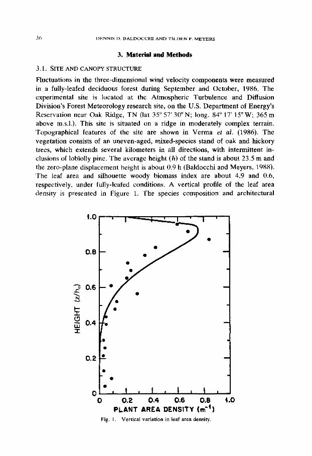
Fluctuations in the three-dimensional wind velocity components were measured in a fully-leafed deciduous forest during September and October, 1986. The experimental site is located at the Atmospheric Turbulence and Diffusion Division’s Forest Meteorology research site, on the U.S. Department of Energy’s Reservation near Oak Ridge, TN (lat 3.5” 57’ 30”N; long. 84” 17’ 15” W; 365 m above m.s.1.). This site is situated on a ridge in moderately complex terrain. Topographical features of the site are shown in Verma er al. (1986). The vegetation consists of an uneven-aged, mixed-species stand of oak and hickory trees, which extends several kilometers in all directions, with intermittent in- clusions of loblolly pine. The average height (h) of the stand is about 23.5 m and the zero-plane displacement height is about 0.9 h (Baldocchi and Meyers, 1988). The leaf area and silhouette woody biomass index are about 4.9 and 0.6, respectively, under fully-leafed conditions. A vertical profile of the leaf area density is presented in Figure 1. The species composition and architectural

4.0

0.6

0

0 I * I I I 0 0.2 0.4 0.6 0.6 4.0

PLANT AREA DENSITY h-‘1 Fig. 1. Vertical variation in leaf area density.


characteristics of the stand are described in Hutchison et al. (1986). The characteristic lengths of the tree crowns are on the order of about 8 to 10 m. The length scale of the leaves is on the order of 0.10 to 0.15 m.

3.2 INSTRUMENTATION

Three uvw sonic anemometers (Applied Technology Inc. Boulder, CO, model BH-478B/3) were used to measure wind velocity components within and above the canopy. The sonic anemometry is discussed in detail in Baldocchi and Meyers (1988). A Gill uvw propeller (R. M. Young, Traverse City, MI) anemometer was also used to measure wind velocity components above the canopy. The propeller anemometers were fitted with extension shafts, as recommended by Hicks (1972). Temperature fluctuations were measured above the canopy with a microbead thermistor, placed next to the anemometry.

The sonic anemometers were supported on swivel-booms, that were attached to a 33 m tall triangular tower. Access to the instruments was provided by an adjacent 44 m tall walk-up tower. The azimuthal angle of the anemometer booms was oriented so the wind generally flowed into the sensor heads, minimizing transducer shadowing effects (Wyngaard and Zhang, 1985). The sensor heads extended about 3 m upwind of the tower to minimize ‘tower shadowing effects’.

We were unable to measure wind velocities simultaneously at all desired levels within the canopy. Consequently, several experiments were conducted with different instrument configurations. Wind velocities were measured above the canopy, at 34 m, with the Gill uvw anemometer during each experimental run to provide reference measurements of ambient wind conditions and heat flux.

Transducer signals were sampled and digitized at a rate of 7.6 Hz with a computer-controlled data acquisition system. Instantaneous data were put on a magnetic disk.

The data presented in this analysis were from daytime periods when wind speed at 34 m exceeded 1.0 m s-i. The predominant wind direction was southwesterly, ranging between about 200 and 260 deg. Atmospheric stability ranged from near neutral to slightly unstable.

3.3 COMPUTATIONAL PROCEDURES

Power and co-spectra and auto and cross lag-correlations were computed with the fast Fourier transform (PIT) technique, using a program by Carter and Ferrie (1979); the FFT program tapered the time series at the ends and removed linear trends. FFT computations were based on a time series of 4096 points. A one-dimensional coordinate rotation was performed on wind data measured within the canopy, making the mean lateral velocity component equal to zero. A three-dimensional coordinate rotation was performed on the velocity components measured above the canopy, forcing the mean w and u values to zero.

The raw spectral densities were block-averaged to provide smoothed estimates over logarithmic frequency bands. The spectral densities presented in this paper


are multiplied by natural frequency, n, and are normalized by their respective variance. They are plotted against the ratio between natural frequency (n) and the local mean horizontal wind velocity (u), an estimate of wavenumber (k). The normalized spectral densities were averaged from many 539 s periods (12 to 40). This ensemble-averaging increases the degree of freedom associated with the spectral computations and reduces the random noise and standard errors associated with spectral estimates from individual experimental runs.

The cross-correlations were normalized by the product of the standard devia- tions of the two velocity measurements. They are plotted against time lags normalized by above-canopy wind speed and vertical separation distance between the two instruments (t = ru/Az). A negative T indicates that wind velocities measured in the canopy lead those measured above, and a positive 7 represents the converse.

4. Results and Discussion

4.1 POWER SPECTRA

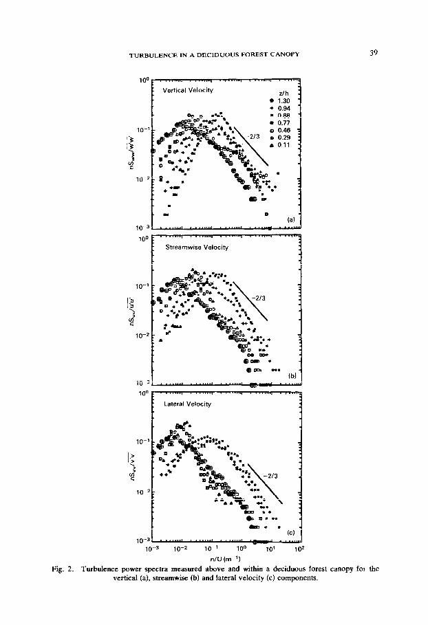
Power spectra for the w, ZJ and u wind velocity components at different levels within and above the deciduous forest are presented in Figures 2a, 2b and 2c, respectively. These power spectra do not collapse upon a universal curve, but are distributed into three regimes. The first regime consists of measurements made above the canopy. The second regime consists of measurements made in the subcanopy trunkspace, below crown closure, and the third regime consists of measurements made in the canopy crown, between 0.75h and h, where h is canopy height. The characteristics of each regime are discussed below.

The turbulence spectra in the surface layer are composed of three subranges: the energy-containing subrange, the inertial subrange and the dissipation subrange (Panofsky and Dutton, 1984). The turbulence spectra measured above the canopy have the shape of a hump, which is representative of energy- containing and inertial subranges; the dissipation subrange is beyond the resolu- tion of the instruments. Peak spectral densities occur at wavenumbers ranging between 0.005 and 0.02 m-‘, which based on Taylor’s frozen eddy hypothesis, corresponds to length scales ranging between 50 and 200m. Hence, these peak values occur in the energy-containing subrange, which is typically associated with length scales on the order of 10 to 2000 m (Panofsky and Dutton, 1984). Among the individual velocity spectra, the peak values rank as: w > u 2 u.

The general shape and ranking of the spectral peaks are in agreement with spectra measured over tall vegetation (Anderson et al., 1986) and short, wheat stubble (Kaimal et al., 1972). The w spectrum peaks at higher wavenumbers than do the horizontal velocity spectra. This is because vertical velocity fluctuations predominately scale with the height above the surface, whereas horizontal velocity fluctuations are influenced by the scale of the terrain features and the height of the planetary boundary layer (Panofsky, 1973; Caughey, 1982).


Vertical Velocity z/h l 1.30 l 0.94

@ma m..

10--a

Lateral Velocity

10-l

1:; r -5 c/f c

10--s :

- . . * m...

* + l I-S

10-3 * *.***"' * *a**...' , 'B ' * **.a

10-3 10-Z 10-I 100 10’ 102

n/U (m-l)

Fig. 2. Turbulence power spectra measured above and within a deciduous forest canopy for the vertical (a), streamwise (b) and lateral velocity (c) components.


In the surface boundary layer, the length scales of turbulence in the inertial subrange range between that of the measurement height above the surface (2) and the Kolmogorov microscale (Panofsky and Dutton, 1984; Jensen and Busch, 1982). In this waveband, no external energy enters the system, nor is any internal energy dissipated; turbulent kinetic energy only cascades from larger to smaller scales. According to Kolmogorov’s scaling theory, the spectral densities of the velocity components in the inertial subrange are a function of the dissipation rate (E) and the wavenumber (k) (see Jensen and Busch, 1982):

(14)

where CY,, is a constant. Velocity spectra measured above the canopy (at 1.30h) have an inertial

subrange with a statistically significant -2/3 slope (Figure 2; Table I), thus, scaling according to Kolmogorov’s theory. These data agree with prior tur-

TABLE 1 Slopes of the velocity spectra at wavenumbers exceeding the spectral peak or the plateau, as observed in the subcanopy trunkspace. r2 is the coefficient of determination and S.E. is the standard error of the estimate of the slope. The question mark (?) indicates data with which we have little confidence

due to high variability and a limited number of data

z/h Velocity component

Slope r2 S.E.

0.11 w u V

0.29 w u V

0.46 w u v

0.77 w u V

0.88 w u V

0.94 w u ”

1.30 W u ”

-0.83 0.96 -0.82 0.7s --I.13 0.89

-0.96 0.99 ~0.89 0.97 -0.86 (?) 0.81

-0.81 0.99 - I .07 0.97 - 1.14 0.96

-0.89 0.97 -1.09 0.99 --0.98 0.99

-1.21 0.99 -- 1.09 0.99 - 1.29 0.98

--0.8X 0.99 --0.70 0.98 - 0.9 1 0.99

-0.68 0.98 -0.66 0.98 -0.66 0.98

0.050 0.011 0.15

0.029 0.067 0.205

0.010 0.073 0.108

0.036 0.023 0.025

0.021 0.032 0.052

0.029 0.032 0.020

0.023 0.02 1 0.020


loo Vett$a~!e~ocity

.

10-l

i 5 .

E 9

Id2

1o-3

+t

log3 loo2 10" loo 10'

n/U (mm')

Fig. 3. Vertical velocity spectrum measured in the canopy crown at 0.88/z.

bulence measurements made over tall vegetation (Anderson ef al., 1986; Thompson, 1979) and short wheat stubble (Kaimal et al., 1972).

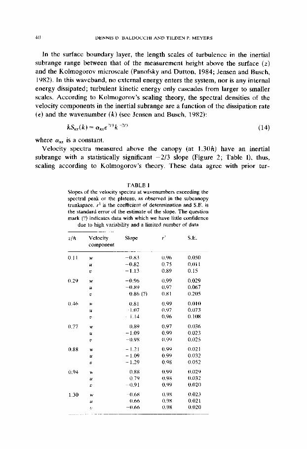
The power spectra measured in the canopy crown are also hump-shaped, but generally exhibit a sharper peak than do these measured above the canopy (Figure 2). This spectral shape is seen more clearly using an individual spectrum sampled from Figure 2; as an example, the vertical velocity power spectrum measured at 0.8Sh is presented in Figure 3. The peak wavenumbers, among the velocity components measured in the canopy crown, rank approximately as w 2 u > u and range between about 0.1 and 0.2 m-r. These peak values are about a decade larger than those from above the canopy.

The spectral slopes in the band of wavenumbers classically associated with the inertial subrange (k > l/z) are significantly more negative than -2/3 in the canopy crown (Figures 2 and 3; Table I). These spectral slopes range between


about -0.78 and - 1.3 (Table I), with the greatest slopes occurring at about 0.88h, where the foliage density and, hence, form drag are greatest (see Figure I). Confidence intervals computed from the standard error of these slopes show that they are all significantly different from -2/3.

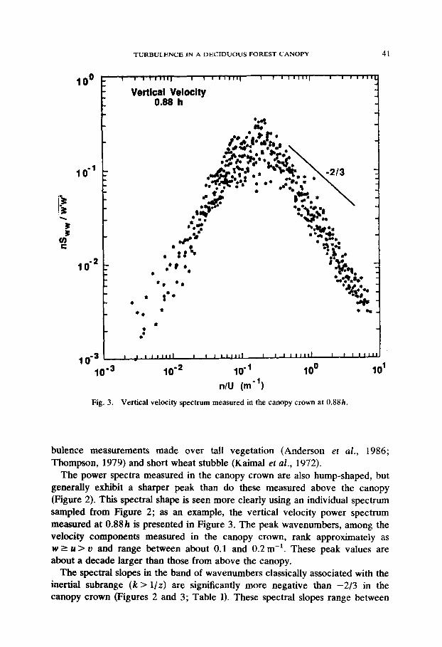
The shape of the velocity spectra measured below crown closure is more complex than are those observed in the other two regimes (see Figure 2); Figure 4 shows a sample vertical velocity spectrum measured at 0.46h in order to examine the features of these spectra in greater detail. The lower-level, power spectra have a distinct peak at wavenumbers ranging between 0.01 and 0.02 m-l nnd also rank as w 2 u > U. At wavenumbers exceeding the peak, the shape of these lower-level spectra differ from those observed at higher levels. First, a rapid drop-off in spectral densities occurs in the region between the spectral peak and wavenumbers on the order of about 0.2 m-‘. Thereafter, the spectral slopes

loo

10-l

-3 -3

2 c2

lo-*

1o-3 ,

.

1o’3 lo-* 10-l loo 10'

n/U (m”) Fig. 4. Vertical velocity spectrum measured below crown closure at 0.46h.


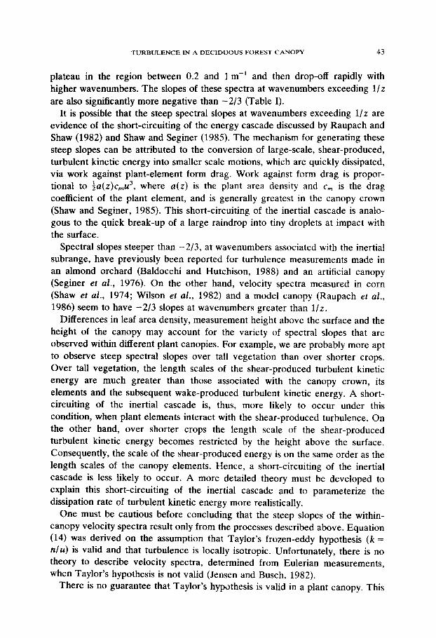
plateau in the region between 0.2 and 1 m-l and then drop-off rapidly with higher wavenumbers. The slopes of these spectra at wavenumbers exceeding l/z are also significantly more negative than -2/3 (Table I).

It is possible that the steep spectral slopes at wavenumbers exceeding l/z are evidence of the short-circuiting of the energy cascade discussed by Raupach and Shaw (1982) and Shaw and Seginer (1985). The mechanism for generating these steep slopes can be attributed to the conversion of large-scale, shear-produced, turbulent kinetic energy into smaller scale motions, which are quickly dissipated, via work against plant-element form drag. Work against form drag is proportional to &(z)c,u3, where a(z) is the plant area density and c, is the drag coefficient of the plant element, and is generally greatest in the canopy crown (Shaw and Seginer, 1985). This short-circuiting of the inertial cascade is analo- gous to the quick break-up of a large raindrop into tiny droplets at impact with the surface.

Spectral slopes steeper than -2/3, at wavenumbers associated with the inertial subrange, have previously been reported for turbulence measurements made in an almond orchard (Baldocchi and Hutchison, 1988) and an artificial canopy (Seginer et al., 1976). On the other hand, velocity spectra measured in corn (Shaw et al., 1974; Wilson et al., 1982) and a model canopy (Raupach et al., 1986) seem to have -2/3 slopes at wavenumbers greater than l/z.

Differences in leaf area density, measurement height above the surface and the height of the canopy may account for the variety of spectral slopes that are observed within different plant canopies. For example, we are probably more apt to observe steep spectral slopes over tall vegetation than over shorter crops. Over tall vegetation, the length scales of the shear-produced turbulent kinetic energy are much greater than those associated with the canopy crown, its elements and the subsequent wake-produced turbulent kinetic energy. A short- circuiting of the inertial cascade is, thus, more likely to occur under this condition, when plant elements interact with the shear-produced turbulence. On the other hand, over shorter crops the length scale of the shear-produced turbulent kinetic energy becomes restricted by the height above the surface. Consequently, the scale of the shear-produced energy is on the same order as the length scales of the canopy elements. Hence, a short-circuiting of the inertial cascade is less likely to occur. A more detailed theory must be developed to explain this short-circuiting of the inertial cascade and to parameterize the dissipation rate of turbulent kinetic energy more realistically.

One must be cautious before concluding that the steep slopes of the within- canopy velocity spectra result only from the processes described above. Equation

(14) was derived on the assumption that Taylor’s frozen-eddy hypothesis (k = n/u) is valid and that turbulence is locally isotropic. Unfortunately, there is no theory to describe velocity spectra, determined from Eulerian measurements, when Taylor’s hypothesis is not valid (Jensen and Busch, 1982).

There is no guarantee that Taylor’s hypothesis is valid in a plant canopy. This


hypothesis can be tested either by comparing whether a fixed-point, Eulerian spectrum (S( nl u)) equals a wavenumber spectrum (S(k)), determined by moving a sensor quickly through the canopy, or by observing that longitudinal coherence values equal one, at all wavenumbers (Panofsky and Dutton, 1984).

Although such measurements are either impossible to make or are unavailable, we can probably assume that Taylor’s hypothesis is not valid in a plant canopy. This is because Taylor’s hypothesis breaks down when turbulence intensities are large and when wind shear is great (Jensen and Busch, 1982), conditions which commonly occur in plant canopies (Wilson et al., 1982; Baldocchi and Meyers, 1988).

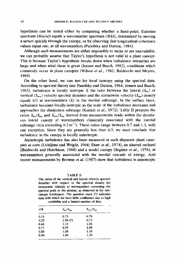
On the other hand, we can test for local isotropy using the spectral data. According to spectral theory (see Panofsky and Dutton, 1984; Jensen and Busch, 1982), turbulence is locally isotropic if the ratio between the lateral (S,,) or vertical (S,,) velocity spectral densities and the streamwise velocity (S,,,) density equals 4/3 at wavenumbers (k) in the inertial subrange. In the surface layer, turbulence becomes locally-isotropic as the scale of the turbulence decreases and approaches the dissipation subrange (Kaimal et al., 1972). Table II presents the ratios S,,/S,,, and S,,/S,, derived from measurements made within the deciduous forest canopy at wavenumbers classically associated with the inertial subrange (n/u exceeding 0.2 m-l). These ratios range between 0.7 and 1.3, with one exception. Since they are generally less than 4/3, we must conclude that turbulence in the canopy is locally anisotropic.

Anisotropic turbulence has also been measured in such disparate plant canopies as corn (Uchijima and Wright, 1964; Shaw et al., 1974), an almond orchard (Baldocchi and Hutchison, 1988) and a model canopy (Seginer et al., 1976), at wavenumbers generally associated with the inertial cascade of energy. And recent measurements by Browne et al. (1987) show that turbulence is anisotropic

TABLE II The ratios of the vertical and lateral velocity spectral densities with respect to the spectral density for streamwise velocity at wavenumbers exceeding the spectral peak or the plateau, as observed in the subcanopy trunkspace. The question mark (?) indicates data with which we have Little confidence due to high

variability and a limited number of data

z/h s*“lL LVIL

0.11 0.75 0.79 0.29 1.94 (?) 0.73 0.46 1.13 1.06 0.77 0.95 1.08 0.88 1.08 1.19 0.94 1.06 1.29


Streamwise Velocity

Fig. 5

.-. .

-@ (cl lo-38

10-a 10-Z 10-l loo 10’ 102

nL,IU . Turbulence power spectra plotted against natural frequency normalized by three wind velocity components measured above and within a deciduous forest

L,IU for the canopy.

46 DENNIS D. BALDOCCHI AND ‘TILDEN P. MEYERS

in the dissipation subrange of turbulent wakes. Based on the evidence at hand, we conclude that the steep spectral slopes observed in the deciduous forest are representative of a combination of effects: the short-circuiting of the inertial cascade of shear-produced turbulent kinetic energy and the invalidity of Taylor’s hypothesis.

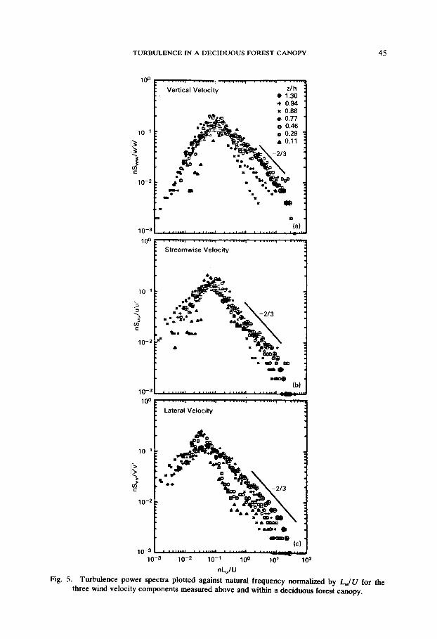
Over the past 15 years there has been much discussion about a meaningful way to non-dimensionalize velocity spectra measured in plant canopies. Silversides (1974) recommended an arbitrary length scale that happened to be close to the average spacing between plants or trees. We feel that a length scale that integrates the scale of the characteristic turbulence, as influenced by the foliage density and distribution and height above the surface, should be used in this normalization. One likely candidate is the Eulerian length scale L,, (Equation 12). Velocity spectra are scaled against a non-dimensional frequency expressed as f=nLiU (Fg i ures Sa, Sb and 5c) for the w, u and u components, respectively (note: this normalization is also equivalent to f = T,,,n). The w and u spectra collapse to a relatively universal spectral peak, occurring at about 0.1. The u spectra collapse at a slightly smaller value. The shape of these spectra, however, are not quite universal; u spectra scaling has the greatest success, whereas u spectra scaling has the least. The lack of a universal spectrum with this normalization, leads us to suggest that two or more length scales may be needed to normalize the within-canopy turbulence spectra. Perhaps one length scale should be attributed to the larger, shear-produced turbulence and another should be representative of the smaller, wake-generated turbulence.

4.2 COSPECTRA

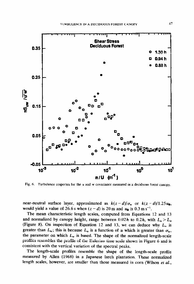
Cospectra between the u and w velocity components are presented in Figure 6 for measurements made above the canopy and at two levels in the crown. The above-canopy cospectrum attains a peak at about 0.01 m-l, whereas the spectral peaks for measurements made in the canopy crown are about a decade higher. Furthermore, the spectral peak shifts toward higher wavenumbers with depth into the canopy, as a result of increasing canopy density and form drag.

Wavenumbers greater than about 0.3 m-l contribute little to tangential momentum stress above and within the canopy. These data support the con- clusion of Lumley and Panofsky (1964), who state that small eddies have considerable energy but do not contribute significantly to the u-w covariance.

4.3. LENGTH ANDTIMESCALES

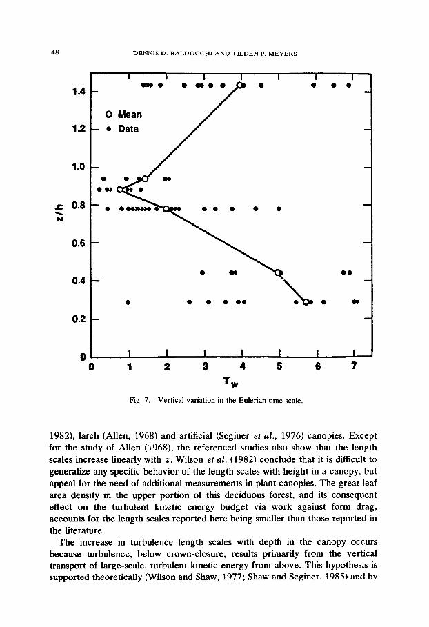
Mean Eulerian time scales (T,) decrease with depth into the canopy until a minima is reached at about 0.88h, where foliage density is greatest (Figure 7). They then increase as z decreases further. Mean time scales range between 0.7 and 5.75 s, with appreciable run-to-run variability due to different wind speed regimes. These time scales are considerably smaller than values observed at similar heights in the surface boundary layer. For example, a time scale in the


0.35

Shear Stress Deciduous Forest

0

0 1.3Oh 0 034 h . 0.88 h

0.25 0

I t

i 9 0.15

0.05

0.05

l 0

O0 0

m OO

00 o” 0

0

0 “0’ OD

ODPO 0

000 O 0 0 0 0 0

0. 0 . = 0

3 a.‘@

0 0

,nm 0

L 0 - O”O

01 oO”G

0 0

109 log2 ltf’ loo lol

n/U (m?) Fig. 6. Turbulence cospectra for the u and w covariance measured in a deciduous forest canopy.

near-neutral surface layer, approximated as k(z - d)/w, or k( z - d)/l.25 w, would yield a value of 26.6 s when (z - d) is 20 m and r+ is 0.3 m SC’.

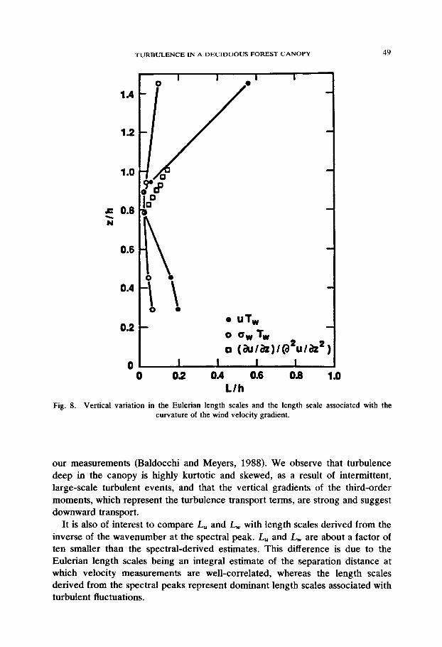
The mean characteristic length scales, computed from Equations 12 and 13 and normalized by canopy height, range between 0.02h to 0.2h, with JY,, > L, (Figure 8). On inspection of Equation 12 and 13, we can deduce why L, is greater than L,,,.; this is because JY,, is a function of u which is greater than a,,,, the parameter on which JL,,, is based. The shape of the normalized length-scale profiles resembles the profile of the Eulerian time scale shown in Figure 6 and is consistent with the vertical variation of the spectral peaks.

The length-scale profiles resemble the shape of the length-scale profile measured by Allen (1968) in a Japanese larch plantation. These normalized length scales, however, are smaller than those measured in corn (Wilson et al.,


1.4

19

1.0

L: 0.8 N N

0.8

0.4

0.2

0

I I I I I I I

omo

0 ~00

P

l 0 0 0

0

- 0

0

l U

- 0

-

I I I I I I I -

0 1 2 3 4 5 6 7

Fig. 7. Vertical variation in the Eulerian time scale.

1982), larch (Allen, 1968) and artificial (Seginer et al., 1976) canopies. Except for the study of Allen (1968), the referenced studies also show that the length scales increase linearly with z. Wilson er al. (1982) conclude that it is difficult to generalize any specific behavior of the length scales with height in a canopy, but appeal for the need of additional measurements in plant canopies. The great leaf area density in the upper portion of this deciduous forest, and its consequent effect on the turbulent kinetic energy budget via work against form drag, accounts for the length scales reported here being smaller than those reported in the literature.

The increase in turbulence length scales with depth in the canopy occurs because turbulence, below crown-closure, results primarily from the vertical transport of large-scale, turbulent kinetic energy from above. This hypothesis is supported theoretically (Wilson and Shaw, 1977; Shaw and Seginer, 1985) and by


0.6

0.4

02

0

0 UT, m 0 %v%u 0 (aJ/az)/@‘u/iR~

0 0.2 0.4 0.6 Od 1.0 L/h

Fig. 8. Vertical variation in the Eulerian length scales and the length scale associated with the curvature of the wind velocity gradient.

our measurements (Baldocchi and Meyers, 1988). We observe that turbulence deep in the canopy is highly kurtotic and skewed, as a result of intermittent, large-scale turbulent events, and that the vertical gradients of the third-order moments, which represent the turbulence transport terms, are strong and suggest downward transport.

It is also of interest to compare L, and I.,,, with length scales derived from the inverse of the wavenumber at the spectral peak. L, and L, are about a factor of ten smaller than the spectral-derived estimates. This difference is due to the Eulerian length scales being an integral estimate of the separation distance at which velocity measurements are well-correlated, whereas the length scales derived from the spectral peaks represent dominant length scales associated with turbulent fluctuations.

50 DENNIS D BALDOCCHI AND TILDEN P. MEYERS

Corrsin ( 1974) reports that gradient transport or ‘K-theory’ models are applic- able if the length scale of the turbulence (L) is much less than the length scale associated with the curvature of the profile of a scalar: L 4 ((du/dz)/(d2u/dz2). He also stipulates that the turbulence length scale must be constant over the distance of a length scale and over the distance for which the mean field of the scalar changes appreciably. In other words, (dL/dz)/L e (du/dz)/u.

Based on Corrsin’s guidelines, Bathe (1986) concludes that ‘K-theory’ momentum transfer models may be valid under limited conditions in the upper portion of some crop canopies. In the micrometeorological literature, ‘K-theory’ has been subject to considerable criticism when used in estimating C02, sensible and latent heat and momentum exchange because turbulence is an intermittent process, the curvature of these scalar profiles is great and counter-gradient transfer can occur (see Finnigan and Raupach, 1987). ‘K-theory’ incorrectly assumes that transfer is linearly proportional to mean gradients and does not admit negative turbulence exchange coefficients.

We can test the validity of ‘K-theory’ when applied to momentum transfer in a forest canopy by comparing length scales computed from the curvature of the wind speed profile against the Eulerian length scales (Figure 8). The curvature length scales, above 0.8h, are about two to three times greater than the Eulerian length scales. According to the strict guidelines established by Corrsin (1974), we conclude that ‘K-theory’ is invalid for estimating momentum transfer in the upper portion of this forest since the differences between the Eulerian and curvature length scales are less than an order of magnitude.

Extending this discussion further, there are some fundamental arguments against the validity of ‘K-theory’ in plant canopies, even under limited conditions. Following Shaw ( 1976), Wilson and Shaw (1977) and Meyers and Paw U (1986), the tangential momentum stress budget under steady-state and neutrally buoyant conditions in an extended, horizontally homogeneous canopy can be expressed as:

-- aw’dlat = 0 - wf2 aulaz - aw’w’dlaz + [ dap’iaz + w’ap’ia] (15)

where p is static pressure and the primes denote fluctuations from the mean. The first term on the RHS is attributed to shear production. The second term represents the convergence of the vertical transfer of tangential momentum stress or turbulent transport. The third term represents the return-to-isotropy due to pressure and velocity interactions. Incorporating a simple parameterization of the -- return-to-isotropy term (w’u’/ tl, where tl is a time scale; Wyngaard, 1982), Equation 15 yields a new equation describing w’u’:

W’U’ = tl[--7* au/az .-- aw’w’dlaz] . (16)

The term, tl?, can be interpreted as being equivalent to a first-order closure, eddy exchange coefficient (K). Therefore, tangential momentum stress inside a


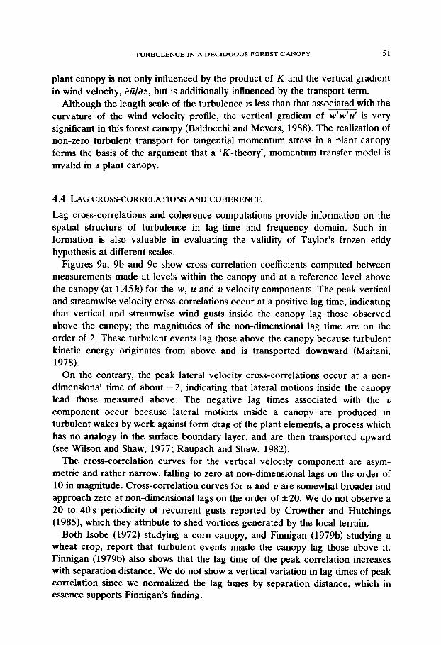
plant canopy is not only influenced by the product of K and the vertical gradient in wind velocity, &3/az, but is additionally intluenced by the transport term.

Although the length scale of the turbulence is less than that associated with the curvature of the wind velocity profile, the vertical gradient of w’ W’U’ is very significant in this forest canopy (Baldocchi and Meyers, 1988). The realization of non-zero turbulent transport for tangential momentum stress in a plant canopy forms the basis of the argument that a ‘K-theory’, momentum transfer model is invalid in a plant canopy.

4.4 LAGCROSS-CORRELAT~ONSANDCOHJZRENCE

Lag cross-correlations and coherence computations provide information on the spatial structure of turbulence in lag-time and frequency domain. Such information is also valuable in evaluating the validity of Taylor’s frozen eddy hypothesis at different scales.

Figures 9a, 9b and 9c show cross-correlation coefficients computed between measurements made at levels within the canopy and at a reference level above the canopy (at 1.45h) for the w, u and u velocity components. The peak vertical and streamwise velocity cross-correlations occur at a positive lag time, indicating that vertical and streamwise wind gusts inside the canopy lag those observed above the canopy; the magnitudes of the non-dimensional lag time are on the order of 2. These turbulent events lag those above the canopy because turbulent kinetic energy originates from above and is transported downward (Maitani, 1978).

On the contrary, the peak lateral velocity cross-correlations occur at a non- dimensional time of about -2, indicating that lateral motions inside the canopy lead those measured above. The negative lag times associated with the u component occur because lateral motions inside a canopy are produced in turbulent wakes by work against form drag of the plant elements, a process which has no analogy in the surface boundary layer, and are then transported upward (see Wilson and Shaw, 1977; Raupach and Shaw, 1982).

The cross-correlation curves for the vertical velocity component are asym- metric and rather narrow, falling to zero at non-dimensional lags on the order of 10 in magnitude. Cross-correlation curves for u and II are somewhat broader and approach zero at non-dimensional lags on the order of +20. We do not observe a 20 to 40s periodicity of recurrent gusts reported by Crowther and Hutchings (1985), which they attribute to shed vortices generated by the local terrain.

Both Isobe (1972) studying a corn canopy, and Finnigan (1979b) studying a wheat crop, report that turbulent events inside the canopy lag those above it. Finnigan (1979b) also shows that the lag time of the peak correlation increases with separation distance. We do not show a vertical variation in lag times of peak correlation since we normalized the lag times by separation distance, which in essence supports Finnigan’s finding.

52 DENNIS D. RAI.DOCCHI AND 7‘ILDFN P. MEYERS

Non-Dimensional Lag, ~.u/Az

Fig. 9. Lag cross-correlations between wind velocity measurements made inside a deciduous forest canopy and at 1.45h.


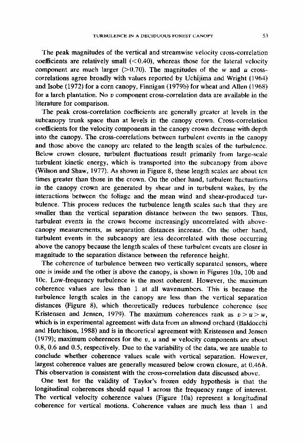
The peak magnitudes of the vertical and streamwise velocity cross-correlation coefficients are relatively small (<0.40), whereas those for the lateral velocity component are much larger (>0.70). The magnitudes of the w and r.~ cross- correlations agree broadly with values reported by Uchijima and Wright (1964) and Isobe (1972) for a corn canopy, Finnigan (1979b) for wheat and Allen (1968) for a larch plantation. No u component cross-correlation data are available in the literature for comparison.

The peak cross-correlation coefficients are generally greater at levels in the subcanopy trunk space than at levels in the canopy crown. Cross-correlation coefficients for the velocity components in the canopy crown decrease with depth into the canopy. The cross-correlations between turbulent events in the canopy and those above the canopy are related to the length scales of the turbulence. Below crown closure, turbulent fluctuations result primarily from large-scale turbulent kinetic energy, which is transported into the subcanopy from above (Wilson and Shaw, 1977). As shown in Figure 8, these length scales are about ten times greater than those in the crown. On the other hand, turbulent fluctuations in the canopy crown are generated by shear and in turbulent wakes, by the interactions between the foliage and the mean wind and shear-produced turbulence. This process reduces the turbulence length scales such that they are smaller than the vertical separation distance between the two sensors. Thus, turbulent events in the crown become increasingly uncorrelated with above- canopy measurements, as separation distances increase. On the other hand, turbulent events in the subcanopy are less decorrelated with those occurring above the canopy because the length scales of these turbulent events are closer in magnitude to the separation distance between the reference height.

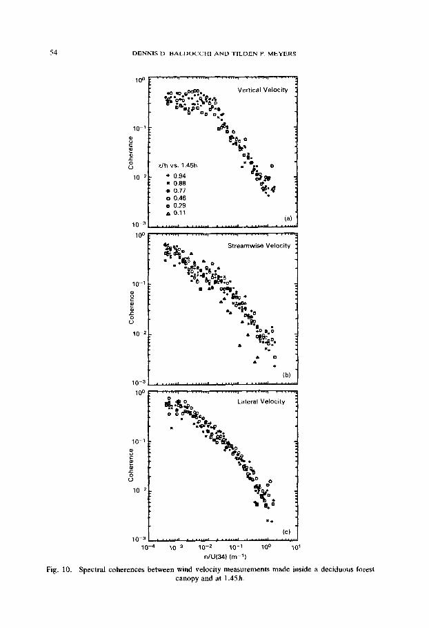
The coherence of turbulence between two vertically separated sensors, where one is inside and the other is above the canopy, is shown in Figures lOa, lob and 10~. Low-frequency turbulence is the most coherent. However, the maximum coherence values are less than 1 at all wavenumbers. This is because the turbulence length scales in the canopy are less than the vertical separation distances (Figure 8), which theoretically reduces turbulence coherence (see Kristensen and Jensen, 1979). The maximum coherences rank as o > u > w, which is in experimental agreement with data from an almond orchard (Baldocchi and Hutchison, 1988) and is in theoretical agreement with Kristensen and Jensen (1979); maximum coherences for the II, u and w velocity components are about 0.8, 0.6 and 0.5, respectively. Due to the variability of the data, we are unable to conclude whether coherence values scale with vertical separation. However, largest coherence values are generally measured below crown closure, at 0.46h. This observation is consistent with the cross-correlation data discussed above.

One test for the validity of Taylor’s frozen eddy hypothesis is that the longitudinal coherences should equal 1 across the frequency range of interest. The vertical velocity coherence values (Figure 10a) represent a longitudinal coherence for vertical motions. Coherence values are much less than 1 and


10 ’ r

z c QO” 2 b’ 2 “4.

8 z/h vs. 1.45h

10-z l 0.94

= 0.88 l 0.77

10-d 10-3 10-Z 10-J 100 10’ n/L&M) (m-l)

Fig. 10. Spectral coherences between wind velocity measurements made inside a deciduous forest canopy and at 1.45 h.


support our earlier contention that Taylor’s hypothesis is not valid in a plant canopy.

5. Summary and Conclusions

The turbulence velocity spectra, presented here, describe the contribution of different frequencies to the variance of velocity fluctuations. Turbulence spectra measured inside a forest canopy are much different than those measured in the surface layer. This is because interactions between wind and plant-parts modify the processes which generate, transport and remove turbulent fluctuations.

We observed that power spectra measured in the canopy crown peak at higher wavenumbers than do those measured in the subcanopy trunkspace and above the canopy. Past attempts to scale within-canopy turbulence spectra have not been very successful. We find that peak spectral values collapse to a relatively universal value when scaled according to a non-dimensional frequency comprised of the product of the natural frequency and the Eulerian time scale for vertical velocity. At wavenumbers exceeding the spectral peak, the slopes of the power spectra are more negative than those observed in the surface boundary layer.

The shift in spectral peaks and the steep spectral slopes result from work against form drag of the plant elements by the mean kinetic energy and the shear-produced turbulent kinetic energy. This work reduces the large-scale energy to that with length scales on the order of the plant elements, which dissipate quickly, thus short-circuiting the inertial cascade. We cannot discount that the steep spectral slopes are also due to the invalidity of Kolmogorov’s scaling arguments for turbulence in the inertial subrange, which are based on the assumptions of Taylor’s frozen eddy hypothesis and local isotropy, because these assumptions are invalid in a plant canopy.

Eulerian length scales in the subcanopy are greater than those in the canopy crown because turbulence at the lower level is primarily due to large-scale, intermittent turbulence transported from above. Turbulent events below crown closure are more correlated with turbulent events above the canopy than are those occurring in the canopy crown because the relative difference between the turbulent length scale and the separation distance is smaller in the subcanopy.

Current theories which describe the turbulent kinetic energy budget must be improved. The weaknesses of these theories revolve around the parameterizations for the dissipation rate of wake-generated turbulence. Hopefully, these data can be used as guidance to improve upon the present models.

The data presented here were from periods with near-neutral to slightly unstable thermal stratification. Additional measurements are needed of turbulence spectra during nocturnal and convective periods to describe the influence of atmospheric stability.


Acknowledgements

This work was supported by the National Oceanic and Atmospheric Ad- ministration and the U.S. Department of Energy. We are grateful to comments provided by Rick Eckman, Ron Dobosy, John Wyngaard and Monique Leclerc regarding different aspects of this work.

References

Allen, L. H., Jr.: 1968, ‘Turbulence and Wind Speed Spectra within a Japanese Larch Plantation’, J. Appl. Meteorol. 7, 73-78.

Anderson, D. E., Verma, S. B., Clement, R. J., Baldocchi, D. D., and Matt, D. R.: 1986, ‘Turbulence Spectra of CO,, Water Vapor, Temperature and Velocity over a Deciduous Forest’, Agric. For. Meteorol. 38, 81-99.

Bathe, D. H.: 1986, ‘Momentum Transfer to Plant Canopies: Influence of Structure and Variable Drag’, Atmospheric Enoironmenf 20, 1369-l 378.

Baldocchi, D. D. and Hutchison, B. A.: 1988, ‘Turbulence in an Almond Orchard: Spatial Variation in Spectra and Coherence’, Boundary- Layer Meteorol. 42, 293-3 11.

Baldocchi, D. D. and Meyers, T. P.: 1988, ‘Turbulence Structure in a Deciduous Forest’, Boundary- Layer Meteorol. 43, 345-365.

Browne, L. W. B., Antonia, R. A., and Shah, D. A.: 1987, ‘Turbulent Energy Dissipation in a Wake’, J. Fluid Mech. 179, 307-326.

Businger, J. A.: 1982, ‘Equations and Concepts’, in F. T. M. Nieuwstadt and H. van Dop (eds.), Armospheric Turbulence and Air Pollution Modeling, D. Reidel Pub. Co., Dordrecht, pp. l-36.

Carter, G. C. and Ferrie, J. F.: 1979, ‘A Coherence and Cross Spectral Estimation Program’, in Digital Processing Committee (eds.), Programs for Digital Signal Processing. IEEE Press, pp. 2.3-l to 2.3-18.

Caughey, S. J.: 1982, ‘Observed Characteristics of the Atmospheric Boundary Layer’, in F. T. M. Nieuwstadt and H. van Dop (eds.), Atmospheric Turbulence and Air Pollution Modeling, D. Reidel Pub. Co., Dordrecht, pp. 107-158.

Corrsin, S.: 1974, ‘Limitations of Gradient Transport Models in Random Walks and in Turbulence’, Ado. Geophys. UA, 25-60.

Crowther, J. M. and Hutchings, N. J.: 1985, ‘Correlated Vertical Wind Speeds in a Spruce Canopy’, in: B. A. Hutchison and B. B. Hicks (eds.), Forest-Atmosphere Interactions, D. Reidel Pub. Co., Dordrecht, pp. 543-562.

Finnigan, J. J.: 1979a, ‘Turbulence in Waving Wheat. I: Mean Statistics and Honami’, Boundary- Layer Meteorol. 16, 181-212.

Finnigan, J. J.: 1979b, ‘Turbulence in Waving Wheat. II: Structure of Momentum Transfer’, Boundary-Layer Meteorol. 16, 213-236.

Finnigan, J. J. and Raupach, M. R.: 1987, ‘Transfer Processes in Plant Canopies in Relation to Stomata1 Characteristics’, in E. Zeiger, G. Farquhar and 1. Cowan (eds.), Stomata1 Function. Stanford University Press, Stanford, CA, pp. 385-429.

Hicks, B. B.: 1972, ‘Propeller Anemometers as Sensors of Atmospheric Turbulence’, Eoundary- Layer Meteorol. 3, 214-228.

Hutch&on, B. A., Matt, D. R., McMillen, R. T., Gross, L. J., Tajchman, S. J., and Norman, J. M.: 1986, ‘The Architecture of an East Tennessee Deciduous Forest Canopy’, J. Ecol. 74, 635646.

Inoue, K.: 1981, ‘A Model Study of Microstructure of Wind Turbulence of Plant Canopy Flow’, Bull. Natl. Inst. Agric. Sci. Ser A. 27,69-89.

Isobe, S.: 1972, ‘A Spectral Analysis of Turbulence in a Corn Canopy’, Bull. Natl. Inst. Agric. Sci. Ser. A. 19, 101-113.

Jensen, N. 0. and Busch, N. E.: 1982, ‘Atmospheric Turbulence’, in E. J. Plate (ed.), Engineeting Meteorology, Elsevier Sci. Pub., pp. 179-23 1.


Kaimal, .I. C., Wyngaard, J. C., Ixumi, Y., and Cote, 0. R.: 1972, ‘Spectral Characteristics of Surface Layer Turbulence’, Quarr. J. Roy. Metorol. Sot. 98, 563-589.

Kristensen, L. and Jensen, N. 0.: 1979, ‘Lateral Coherence in Isotropic Turbulence and in the Natural Wind’, Boundary-Layer Meteorol. 17, 353-373.

Iegg, B. J. and Raupach, M. R.: 1982, ‘Markov-Chain Simulation of Particle Dispersion in Inhomogeneous Flows: the Mean Drift Velocity Induced by a Gradient in Eulerian Velocity Variance’, Boundary-Layer Meteorol. 24, 3-13.

Lumley, J. L. and Panofsky, H. A.: 1964, The Structure of Atmospheric Turbulence, Interscience, New York, 239 pp.

Maitani, T.: 1978, ‘On the Downward Transport of Turbulent Kinetic Energy in the Surface Layer over Plant Canopies’, Boundary-Layer Meteorol. 14, 571-584.

Meyers, T. P. and Paw U. K. T.: 1986, ‘Testing of a Higher Order Closure Model for Modeling AirfIow within and above Plant Canopies’, Boundary-Layer Meteorol. 37, 297-3 11.

Panofsky, H. A.: 1973, ‘Tower Micrometeorology’, in D. A. Haugen (ed.), Workshop on Micro- me&orology, American Meteorological Society, Boston, pp. 151-176.

Panofsky, H. A. and Dutton, J. A.: 1984, Atmospheric Turbulence: Models and Methods for Engineeting Applications, John Wiley and Sons, New York, 397 pp.

Raupach, M. R.: 1987, ‘A Lagrangian Analysis of Scalar Transfer in Vegetation Canopies’, Quart. J. Roy. Meteorol. Sot. 113, 107-120.

Raupach, M. R. and Shaw, R. H.: 1982, ‘Averaging Procedures for Flow within Vegetation Canopies’, Boundary-Layer Meteorol. 22, 79-90.

Raupach, M. R., Coppin, P. A., and Legg, B. J.: 1986, ‘Experiments on Scalar Dispersion within a Model Plant Canopy, Part 1: The Turbulent Structure’, Boundary-Layer Meteorol. 35, 21-52.

Seginer, I., Mulbeam, P. J., Bradley, E. F., and Finnigan, J. J.: 1976, ‘Turbulent Flow in a Model Plant Canopy’, Boundary-Layer Meteorol. 10, 423-453.

Seginer, I. and Mulheam, P. J.: 1978, ‘A Note on Vertical Coherence of Streamwise Turbulence inside and above a Model Plant Canopy’, Boundary-Layer Meteorol. 14, 515-523.

Shaw, R. H., Silversides, R. H., and Thurtell, G. W.: 1974, ‘Some Observations of Turbulence and Turbulent Transport within and above Plant Canopies’, Boundary-Layer Meteorol. 5, 429-449.

Shaw, R. H.: 1976, ‘Secondary Wind Maxima Inside Plant Canopies’, J. Appl. Meteorol. 16, 514-521. Shaw, R. H. and Seginer, I.: 1985, ‘The Dissipation of Turbulence in Plant Canopies’, 7th Symp. on

Turbulence and Dij@ion, Am. Meteorol. Sot., Boston, pp. 200-203. Silversides, R. H.: 1974, ‘On Scaling Parameters for Turbulence Spectra within Plant Canopies’,

Agric. Meteorol. 13,203-211. Thompson, N.: 1979, ‘Turbulence Measurements Over a Pine Forest’, Boundary-Layer Meteorol. 16,

293-310. Uchijima, Z. and Wright, J. L.: 1964, ‘An Experimental Study of Air Flow in a Corn Plant-air Layer’,

Bull. Natl. Inst. Agric. Sci. Ser A. 11, 19-65. Verma, S. B., Baldocchi, D. D., Anderson, D. E., Matt, D. R., and Clement, R. J.: 1986, ‘Eddy

Fluxes of CO*, Water Vapor and Sensible Heat over a Deciduous Forest’, Bout&q+Layer Meteorol. 36, 71-91.

Weiss, A. and Allen, L. H., Jr.: 1976, ‘Air Flow Patterns in Vineyard Rows’, Agric. Meteorol. 16, 329-342.

Wilson, J. D., Thurtell, G. W., and Kidd, G. E.: 1981, ‘Numerical Simulation of Particle Trajectories in Inhomogeneous Turbulence, I: Systems with Constant Turbulent Velocity Scales’, Boundary- Layer Meteorol. 21, 295-313.

Wilson, J. D., Thurtell, G. W., and Kidd, G. E.: 1981, ‘Numerical Simulation of Particle Trajectories in Inhomogeneous Turbulence, I: Systems with Constant Turbulent Velocity Scales’, Boundary- Layer Meteorol. 21,295-3 13.

Wilson, J. D., Ward, D. P., Thurtell, G. W., and Kidd, G. E.: 1982, ‘Statistics of Atmospheric Turbulence within and above a Corn Canopy’, Boundary-Layer Meteorol. 24,495-519.

Wilson, N. R. and Shaw, R. H.: 1977, ‘A Higher Order Closure Model for Canopy Flow’, J. A@. Meteorol. 16, 1197-1205.

Wyngaard, J. C.: 1982, Boundary Layer Modeling’, in F. T. M. Nieuwstadt and van Dop (eds.),


Atmospheric Turbulence and Air Pollution Modeling, D. Reidel Pub. Co., Dordrecht, pp. 69-106. Wyngaard, J. C. and Zhang, S. F.: 1985, ‘Transducer-Shadow Effects on Turbulence Spectra

Measured by Sonic Anemometers’, J. Atmos. Oceanic Tech. 2, 548-558. Yamada, T.: 1982, ‘A Numerical Model Study of Turbulent Airflow in and Above a Forest Canopy’,

J. Meteorol. Sot. Japan. 60, 439-454. Yamada, T.: 1982, ‘A Numerical Model Study of Turbulent Airflow in and Above a Forest Canopy’,

J. Meteorol. Sot. Japan. 60, 439-454.

Documents

DENNIS D. BALDOCCHI and TILDEN P. MEYERS