Real-Time SystDOI 10.1007/s11241-009-9087-4

DESH: overhead reduction algorithms for deferrablescheduling

Ming Xiong · Song Han · Deji Chen ·Kam-Yiu Lam · Shan Feng

© Springer Science+Business Media, LLC 2009

Abstract Although the deferrable scheduling algorithm for fixed priority transac-tions (DS-FP) has been shown to be a very effective approach for minimizing real-time update transaction workload, it suffers from its on-line scheduling overhead. Inthis work, we propose two extensions of DS-FP to minimize the on-line schedulingoverhead. The proposed algorithms produce a hyperperiod from DS-FP so that theschedule generated by repeating the hyperperiod infinitely satisfies the temporal va-lidity constraint of the real-time data. The first algorithm, named DEferrable Schedul-ing with Hyperperiod by Schedule Construction (DESH-SC), searches the DS-FPschedule for a hyperperiod. The second algorithm, named DEferrable Schedulingwith Hyperperiod by Schedule Adjustment (DESH-SA), adjusts the DS-FP schedule

M. XiongBell Labs, Alcatel-Lucent, 600 Mountain Avenue, Murray Hill, NJ 08807, USAe-mail: xiong@research.bell-labs.com

S. Han (�)Department of Computer Sciences, University of Texas at Austin, 1 University Station C0500,Taylor Hall 2.124, Austin, TX 78712-1188, USAe-mail: shan@cs.utexas.edu

D. ChenEmerson Process Management, 12301 Research Blvd # 3, Austin, TX 78759-2369, USAe-mail: Deji.Chen@EmersonProcess.com

K.-Y. LamDepartment of Computer Science, City University of Hong Kong, 83 Tat Chee Avenue, Kowloon,Hong Konge-mail: cskylam@cityu.edu.hk

S. FengThe Mathematics and Software Science College, Sichuan Normal University, 610068 Chengdu,Sichuan, Chinae-mail: fengs@sicnu.edu.cn

Real-Time Syst

in an interval to form a hyperperiod. Our experimental results demonstrate that whileboth DESH-SC and DESH-SA can reduce the scheduling overhead of DS-FP, DESH-SA outperforms DESH-SC by accommodating significantly more update transactionsin the system. Moreover, DESH-SA can also achieve near-optimal update workload.

Keywords Real-Time databases · Temporal validity constraint · Fixed priorityscheduling · Deferrable scheduling

1 Introduction

Real-time embedded systems are important components of many time-critical ap-plications that require timely processing of massive amount of real-time data. Thecorrect functioning of a real-time embedded system depends not only on meetingreal-time constraints of application jobs, but also on the accuracy of real-time datavalues sampled from real-world entities. Examples of real-time data include sensordata in sensor networks, positions of aircrafts in air traffic control systems, and vehi-cle velocity in adaptive cruise control applications. To provide better management ofsampled real-time data and to support effective processing of application jobs, real-time data are typically managed by a real-time database system (RTDBS). passage oftime since the status of the corresponding entity in the real-world may change contin-uously. Sensor update transactions should constantly sample real-world data valuesand install them into the RTDBS.

One efficient way to determine the correctness of real-time data in a RTDBS is todefine a validity constraint (Song and Liu 1995; Ramamritham 1993; Kuo and Mok1992, 1993; Ho et al. 1997; Gerber et al. 1994; Xiong et al. 2002, 2005; Kang et al.2002; Lam et al. 2004; Gustafsson and Hansson 2004a, 2004b; Chen and Mok 2004;Xiong and Ramamritham 2004) or age constraint (Burns and Davis 1996), whichdetermines a validity interval length for each real-time data object. A real-time datavalue is only valid within its validity interval. In practice, for safety and reliabilityreasons, real-time embedded systems require continuous generation of update trans-actions to refresh real-time data objects regardless of how much the status of thecorresponding real-world entities have been changed. To meet this constraint, it isimportant to produce a schedule for all update transactions such that for any con-secutive updates of a real-time data object, the next update is completed before theprevious validity interval expires. Thus one of the crucial issues in the design of real-time embedded systems is to schedule the update transactions efficiently to maintainthe validity of real-time data while minimizing the total update transaction workload.

Prior work Most of the previous work in update transaction scheduling assumeda periodic transaction model. The update problem for periodic update transactionsconsists of two parts (Xiong and Ramamritham 2004): (1) the determination of thesampling periods and deadlines of update transactions; and (2) the scheduling of up-date transactions. One of the proposed approaches is the Half-Half (HH) scheme(Ramamritham 1993; Ho et al. 1997) in which an update transaction has a fixedperiod that is half of the validity interval. If the set of transactions is schedulable

Real-Time Syst

in HH, the validity constraints of the corresponding real-time data objects can alsobe guaranteed. Similarly to HH, More-Less (ML) (Xiong and Ramamritham 2004;Lam et al. 2004; Chen and Mok 2004) is another periodic approach in which up-date transactions are scheduled based on the deadline monotonic algorithm (Leungand Whitehead 1982). Compared to HH, ML can guarantee the validity of real-timedata objects with less update transaction workload. Recently, the DS-FP algorithmwas proposed (Xiong et al. 2005) to further reduce the total update transaction work-load. The main idea of DS-FP is to adopt sporadic task model instead of the periodicmodel. Compared to ML, DS-FP increases the separation of two consecutive trans-action jobs by releasing an update transaction job as late as possible based on thesampling time of its previous job. Both theoretical analysis and experimental resultshave demonstrated that DS-FP outperforms HH and ML significantly in reducing theupdate transaction workload while still maintaining the real-time data validity.

One major problem of DS-FP is its time complexity for on-line schedule com-putation (Xiong et al. 2005). The variation in its run-time overhead leads to unpre-dictability of the system performance. This paper thus aims at reducing the on-linescheduling overhead of the DS-FP algorithm to constant, which provides more pre-dictability to the system performance. We propose two Deferrable Scheduling withHyperperiod (DESH) algorithms, which construct the hyperperiod schedule off-lineand reduce the on-line scheduling time complexity to O(1).

Contributions The key contributions of our work include the followings.

(1) To reduce on-line scheduling overhead, our first algorithm, named DeferrableScheduling with Hyperperiod Construction (DESH-SC), searches the hyperpe-riod of the set of update transactions so that the transactions can be scheduled byrepeating the hyperperiod schedule. However, the hyperperiods found by DESH-SC are exponentially long, which could incur significant space overhead formaintaining the hyperperiod information for on-line scheduling.

(2) Our second algorithm, named Deferrable Scheduling with Schedule Adjustment(DESH-SA), adjusts the DS-FP schedule in an interval such that the adjustedschedule can be repeated infinitely. DESH-SA improves DESH-SC on producingmuch shorter hyperperiods and accommodating significantly more update trans-actions.

(3) The two DESH algorithms are experimentally studied by simulation, and the pri-mary performance metrics used in our experimental studies are the CPU work-load and the number of transactions supported in the system. Our experimentalresults demonstrate that both DESH-SC and DESH-SA can reduce schedulingoverhead of DS-FP, and DESH-SA outperforms DESH-SC by accommodatingsignificantly more update transactions in the system.

Organization This paper is organized as follows: Sect. 2 briefly reviews the back-ground and related work in the area. Section 3 presents the details of the two proposedalgorithms. Section 4 reports our experimental results of DESH-SC and DESH-SA.Finally, we conclude the paper and discuss the future work in Sect. 5.

Real-Time Syst

2 Background and related work

This section briefly reviews the temporal validity of real-time data, and the More-Less (ML) (Burns and Davis 1996; Xiong and Ramamritham 2004) and deferrablescheduling (DS-FP) (Xiong et al. 2005) algorithms. Formal definitions of the fre-quently used symbols are summarized in Table 1.

Definition 2.1 A real-time data object (Xi ) at time t is temporally valid (or ab-solutely consistent) if, for its j th update finished latest before t , the samplingtime (ri,j ) plus the validity interval (Vi ) of the data object is not less than t , i.e.,ri,j + Vi ≥ t (Ramamritham 1993).

A data value for real-time data object Xi sampled at any time t will be valid upto (t + Vi ). The actual length of the temporal validity interval of a real-time dataobject is application dependent (Ramamritham 1993, 1996; Locke 1997). One of theimportant design goals of RTDBS is to guarantee that real-time data remain fresh,i.e., they are always valid.

We assume that the network delay for a sensor update transaction job to be sentfrom a sensor to the RTDBS (i.e., jitter between sampling time at the sensor and re-lease time at the RTDBS) is zero for convenience of presentation. Our results herecan be easily extended to the case that jitter is non-zero if the maximum jitter of atransaction is known. In the presence of non-zero jitters, we can transform a trans-action τ ′

i (with validity length V ′i and maximum jitter δi ) to a transaction τi (with

validity length Vi = V ′i − δi and zero jitter). Such a transformation guarantees that if

τi can meet its validity constraint, then τ ′i can also meet its validity constraint.

Given a set of transactions T = {τi}mi=1, we assume without loss of generality thatτk has higher priority than τj for k < j .

Table 1 Symbols anddefinitions Symbol Definition

Xi Real-time data object i

τi Update transaction updating Xi (i = 1, . . . ,m)

Ji,j The j th job of τi (j = 0,1,2, . . .)

Ri,j Response time of Ji,j

Ci Computation time of transaction τi

Vi Validity (interval) length of Xi

fi,j Finishing time of Ji,j

ri,j Release (Sampling) time of Ji,j

di,j Absolute deadline of Ji,j

Pi Period of transaction τi in ML

Di Relative deadline of transaction τi in ML

UDS An estimated average CPU utilization in DS-FP

�i(a, b) Total cumulative processor demands from higher-

priority transactions received by τi in interval [a, b)

Real-Time Syst

More-less ML adopts the periodic task model (Leung and Whitehead 1982) for sen-sor update transactions whose derived deadlines are not larger than their periods. Con-sider synchronous transactions whose first jobs all start at time 0. A time instant afterwhich a transaction job has the worst-case response time is called a critical instant,e.g., time 0 is a critical instant for all the transactions with deadlines no larger thantheir periods if those transactions are synchronous (Leung and Whitehead 1982). Notethat we only consider synchronous transactions. In ML, there are three constraints tofollow for transactions τi (∀i, 1 ≤ i ≤ m) (Xiong and Ramamritham 2004):

• Validity constraint: the sum of the period and relative deadline of transaction τi isalways less than or equal to Vi , i.e., Pi + Di ≤ Vi .

• Deadline constraint: the period of an update transaction is assigned to be more thanor equal to half of the validity length of its updated object, while its correspondingrelative deadline is less than or equal to half of the validity length of the sameobject. For τi to be schedulable, Di must be greater than or equal to Ci , the worst-case execution time of τi , i.e., Ci ≤ Di < Pi .

• Schedulability constraint: for a given set of update transactions, the DeadlineMonotonic scheduling algorithm (Leung and Whitehead 1982) is used to sched-ule the transactions. That is,

∑ij=1(�Di

Pj� · Cj ) ≤ Di (1 ≤ i ≤ m).

ML assigns priorities to transactions based on Shortest Validity First (SVF), i.e., inthe inverse order of validity length, and ties are resolved in favor of transactions withlarger computation time (Ci ). It assigns deadlines and periods to τi as follows:

Di = f mli,0 − rml

i,0 , (1)

Pi = Vi − Di, (2)

where f mli,0 and rml

i,0 are the finishing and sampling times of the first job of τi , respec-

tively. Note that in a synchronous system, rmli,0 = 0 and the first job’s response time is

the worst-case response time in ML. We use superscript ml to distinguish the finishingand sampling times in ML from those in DS-FP.

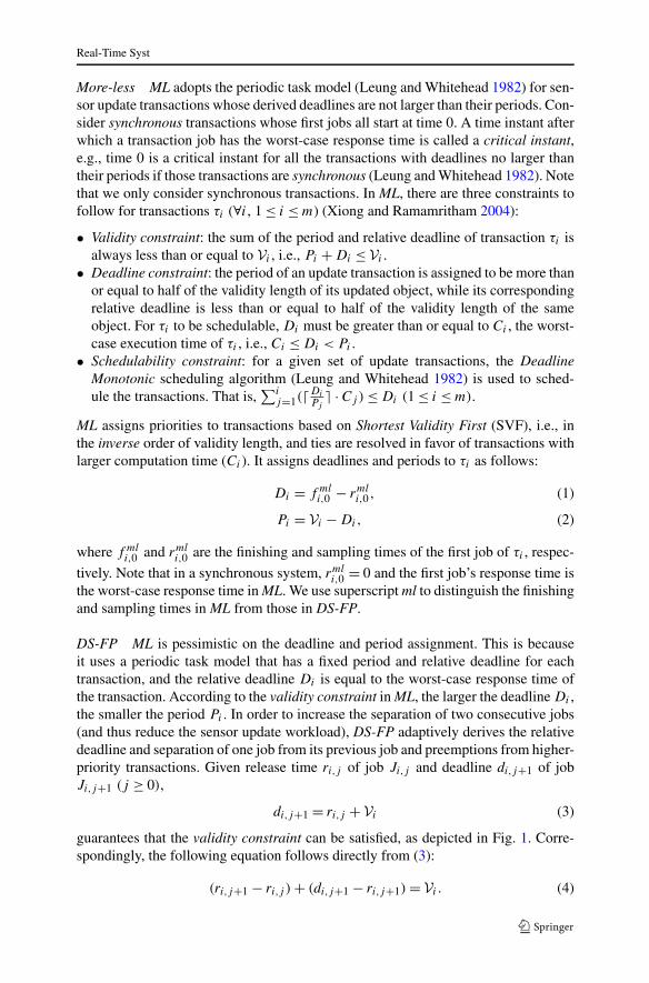
DS-FP ML is pessimistic on the deadline and period assignment. This is becauseit uses a periodic task model that has a fixed period and relative deadline for eachtransaction, and the relative deadline Di is equal to the worst-case response time ofthe transaction. According to the validity constraint in ML, the larger the deadline Di ,the smaller the period Pi . In order to increase the separation of two consecutive jobs(and thus reduce the sensor update workload), DS-FP adaptively derives the relativedeadline and separation of one job from its previous job and preemptions from higher-priority transactions. Given release time ri,j of job Ji,j and deadline di,j+1 of jobJi,j+1 (j ≥ 0),

di,j+1 = ri,j + Vi (3)

guarantees that the validity constraint can be satisfied, as depicted in Fig. 1. Corre-spondingly, the following equation follows directly from (3):

(ri,j+1 − ri,j ) + (di,j+1 − ri,j+1) = Vi . (4)

Real-Time Syst

Fig. 1 Illustration of DS-FP scheduling

If ri,j+1 can be shifted onward to r ′i,j+1 along the time line in Fig. 1, it does not

violate (4). After the shift, temporal validity can still be guaranteed as long as Ji,j+1is completed by its deadline di,j+1. The idea of DS-FP is to defer the sampling time(i.e., release time), ri,j+1, of Ji,j ’s next job as late as possible while still guaranteeingthe validity constraint.

According to the fixed priority scheduling theory, ri,j+1 in DS-FP can be derivedbackwards from its deadline di,j+1 as follows:

ri,j+1 = di,j+1 − Ri,j+1(ri,j+1, di,j+1); (5)

Ri,j+1(ri,j+1, di,j+1) = �i(ri,j+1, di,j+1) + Ci. (6)

where �i(a, b) denotes the total cumulative processor demands made by all jobs ofhigher-priority transaction τk (∀k, 1 ≤ k ≤ i − 1) during time interval [a, b), andRi,j+1(ri,j+1, di,j+1) (or Ri,j+1 for simplicity in DS-FP) the response time of Ji,j+1deriving backwards from its deadline di,j+1. Note that the schedule of all higher-priority jobs that are released prior to di,j+1 needs to be computed before computing�i(ri,j+1, di,j+1).

Similarly to ML, DS-FP also assigns priorities to transactions according to SVF.Readers are referred to the Appendix for the details of the DS-FP algorithm. Now wesummarize the algorithm as follows. First we set ri,0 = 0,∀i,1 ≤ i ≤ m. The highestpriority job among the outstanding jobs is always scheduled first. It is only preemptedwhen a new job with higher priority is ready. As soon as a job Ji,j is completed, wederive the ri,j+1 of its next job according to above calculations. The algorithm failswhen a job misses its deadline. Otherwise it keeps running. It is proved that any taskset that is scheduled by ML is also scheduled by DS-FP (Xiong et al. 2006).

The EDL algorithm proposed in Chetto and Chetto (1989) processes tasks as lateas possible based on the Earliest Deadline algorithm (Liu and Layland 1973). EDLassumes that all deadlines of tasks are given whereas DS-FP and DESH algorithms

Real-Time Syst

derive deadlines dynamically. The validity constrained scheduling, e.g., ML, DS-FP,and DESH algorithms, are different from the distance constrained scheduling, whichguarantees an upper bound to the finishing times of two consecutive instances of atask (Han et al. 1995).

3 Deferrable scheduling with hyperperiod

The DS-FP algorithm is very effective at reducing processor utilization while guar-anteeing the validity constraint. However, its on-line scheduling overhead in terms oftime complexity is much higher than that of ML. Moreover, the scheduling overheadof DS-FP depends on the number of transactions and the validity length of updateddata. Thus, DS-FP can become very expensive, e.g., when the transaction set be-comes large. In contrast to a periodic schedule that has the least common multipleof task periods as its hyperperiod, there is usually no such natural hyperperiod fora DS-FP schedule. Next, we present two DEferrable Scheduling with Hyperperiod(DESH) algorithms for constructing periodic schedules off-line from the DS-FP al-gorithm so that the on-line scheduling time complexity can be reduced. Note that thiswill undoubtedly increase the space overhead for keeping the DESH schedules. Butthe space overhead can be kept reasonably low as demonstrated in our experimentsin Sect. 4. Our DESH algorithms satisfy the following properties:

Property 3.1 A schedule satisfies the validity constraint.

Property 3.2 The on-line scheduling time complexity is O(1).

3.1 DEferrable Scheduling with Hyperperiod: Schedule Construction (DESH-SC)

In this subsection, we present DEferrable Scheduling with Hyperperiod based onSchedule Construction (DESH-SC), a DS-FP based algorithm that can reduce the on-line scheduling overhead. The basic idea of DESH-SC is to search for an interval ofDS-FP schedule, the hyperperiod, that could be repeated infinitely without violatingthe validity constraint. Note that DESH-SC could return without finding a hyperpe-riod.

The DESH-SC algorithm consists of two parts: an algorithm for finding the hy-perperiod off-line (see Algorithm 3.1) and an algorithm for scheduling transactionson-line. The latter is trivial once a hyperperiod is found because it only needs to re-peat the hyperperiod schedule. Therefore, we next describe how the hyperperiod isderived from the schedule of DS-FP.

For a DS-FP schedule and a time period [ts , te], we say [ts , te] is a hyperperiodfor the transaction set if for all transactions τi (1 ≤ i ≤ m), the following schedulesatisfies τi ’s validity constraint: it is the same as the DS-FP schedule from time 0to te . From te onward, it repeats the DS-FP schedule in [ts , te] to infinity. Please notethat ts and te do not need to be idle time points in DESH-SA, which is different fromthe requirements of ts and te in DESH-SC.

Real-Time Syst

Lemma 3.1 [ts , te] is a hyperperiod in DESH-SC if for all τi (1 ≤ i ≤ m) the follow-ing conditions hold.

1. ts and te are CPU idle time points.2. ts > Vi .3. τi is scheduled at least once in [ts , te].4. I (ts, τi) ≥ I (te, τi), where function I (t, τi) is defined as the time distance between

t and τi ’s latest release time before t .

Proof Given any τi (1 ≤ i ≤ m), we first prove in the hyperperiod schedule that thedistance of the finish time of the first τi job after te and the release time of its latestjob before te satisfies the validity constraint. Note that the first job after te repeatsthe first job in [ts , te]. Because ts > Vi , the first job of τi in [ts , te] must finish by(ts − I (ts, τi))+ Vi , in other words, by Vi − I (ts, τi) after ts . Since [ts , te] is repeatedafter te, the first job of τi after te also finishes by Vi − I (ts, τi) after te. The distancebetween the finish time of its first job in the second hyperperiod [te,2te − ts] and therelease time of its latest job in the first hyperperiod [ts , te] is no longer than:

I (te, τi) + (Vi − I (ts, τi)) = Vi + (I (te, τi) − I (ts, τi)) ≤ Vi .

Similarly, we can prove that the distance between the finish time of its first job in the(k + 1)th (k = 1,2, . . .) hyperperiod and the release time of its latest job in the kthhyperperiod is no longer than Vi . Thus, the jobs of τi satisfy the validity constraint. �

Note that the third condition could be derived from the fourth condition: If no jobis scheduled in [ts , te], then τi ’s latest release time before ts is also its latest releasetime before te, hence the fourth condition is always false.

To better satisfy the fourth condition, we need to assign ts to be the end of an idleperiod and te to be the beginning of another idle period. By idle period [t1, t2] wemean that CPU is busy right before t1, it idles between t1 and t2, and it is busy againafter t2. Once the hyperperiod is found, we could increase te as long as the conditionsin Lemma 3.1 are satisfied. The idea is presented in Algorithm 3.1. In the algorithm,we continuously push t2 of idle periods into a queue Q as possible candidates forts of a hyperperiod. For each subsequent idle period, we check its t1 against each t2saved in Q to see if they form a hyperperiod. If the hyperperiod is found, we couldthen further increase te as long as [ts , te] still satisfies the conditions in Lemma 3.1.The increase cannot exceed I (ts, τi) − I (te, τi) for any transaction τi,1 ≤ i ≤ m. Wedefine w to be the minimum of I (ts, τi) − I (te, τi) in the algorithm.

Algorithm 3.1 SearchHyperperiod:

Input: A DS-FP schedule, a utilization limit Umax, and a time limit tmax.Output: The hyperperiod with utilization ≤ Umax.

1 U ← 1.001; // Initialization of hyperperiod utilization.2 t2 ← max{Vi | 1 ≤ i ≤ m};3 [t1, t2] ← first CPU idle period after t2;

Real-Time Syst

4 Append t2 to Q; //Q is a FIFO queue of t2.5 while (U > Umax) do6 [t1, t2] ← next CPU idle period after t2;7 // tmax is the maximum time to search.8 if (t1 > tmax) then return failure; endif9 te ← t1;

10 for ts = first in Q to last in Q do11 if ([ts , te] satisfies Condition 4 in Lemma 3.1)

12 then13 Signal that a hyperperiod exists;14 w ← min{I (ts, τi) − I (te, τi) | 1 ≤ i ≤ m};15 te ← te + min(w, (t2 − t1)); // Fine-tune te.16 U ′ ← utilization in [ts , te];17 if (U > U ′) then18 U ← U ′;19 if (U ≤ Umax) then goto RT N ; endif20 endif21 endif22 end23 if Q is full then Dequeue the oldest; endif24 Append t2 to Q;25 end26 RTN: return [ts , te] as the hyperperiod;

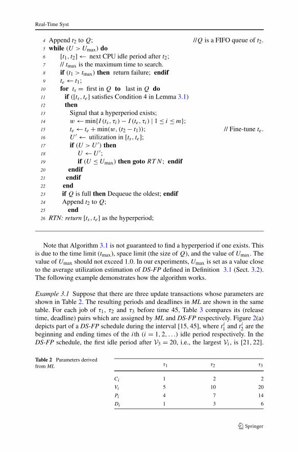
Note that Algorithm 3.1 is not guaranteed to find a hyperperiod if one exists. Thisis due to the time limit (tmax), space limit (the size of Q), and the value of Umax. Thevalue of Umax should not exceed 1.0. In our experiments, Umax is set as a value closeto the average utilization estimation of DS-FP defined in Definition 3.1 (Sect. 3.2).The following example demonstrates how the algorithm works.

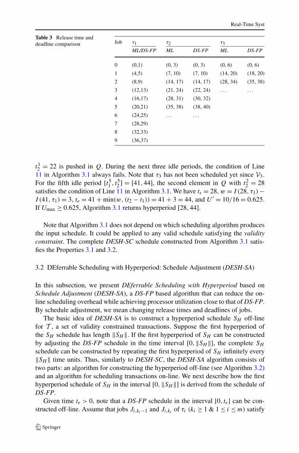
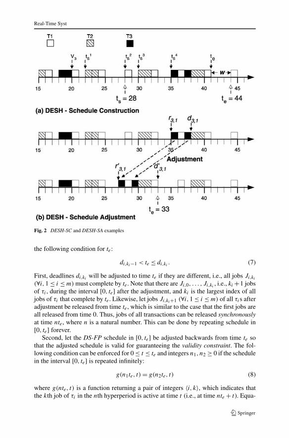
Example 3.1 Suppose that there are three update transactions whose parameters areshown in Table 2. The resulting periods and deadlines in ML are shown in the sametable. For each job of τ1, τ2 and τ3 before time 45, Table 3 compares its (releasetime, deadline) pairs which are assigned by ML and DS-FP respectively. Figure 2(a)depicts part of a DS-FP schedule during the interval [15,45], where t i1 and t i2 are thebeginning and ending times of the ith (i = 1,2, . . .) idle period respectively. In theDS-FP schedule, the first idle period after V3 = 20, i.e., the largest Vi , is [21,22].

Table 2 Parameters derivedfrom ML τ1 τ2 τ3

Ci 1 2 2

Vi 5 10 20

Pi 4 7 14

Di 1 3 6

Real-Time Syst

Table 3 Release time anddeadline comparison Job τ1 τ2 τ3

ML/DS-FP ML DS-FP ML DS-FP

0 (0,1) (0, 3) (0, 3) (0, 6) (0, 6)

1 (4,5) (7, 10) (7, 10) (14, 20) (18, 20)

2 (8,9) (14, 17) (14, 17) (28, 34) (35, 38)

3 (12,13) (21, 24) (22, 24) . . . . . .

4 (16,17) (28, 31) (30, 32)

5 (20,21) (35, 38) (38, 40)

6 (24,25) . . . . . .

7 (28,29)

8 (32,33)

9 (36,37)

t12 = 22 is pushed in Q. During the next three idle periods, the condition of Line

11 in Algorithm 3.1 always fails. Note that τ3 has not been scheduled yet since V3.For the fifth idle period [t5

1 , t52 ] = [41,44], the second element in Q with t2

2 = 28satisfies the condition of Line 11 in Algorithm 3.1. We have ts = 28, w = I (28, τ1)−I (41, τ1) = 3, te = 41 + min(w, (t2 − t1)) = 41 + 3 = 44, and U ′ = 10/16 = 0.625.If Umax ≥ 0.625, Algorithm 3.1 returns hyperperiod [28,44].

Note that Algorithm 3.1 does not depend on which scheduling algorithm producesthe input schedule. It could be applied to any valid schedule satisfying the validityconstraint. The complete DESH-SC schedule constructed from Algorithm 3.1 satis-fies the Properties 3.1 and 3.2.

3.2 DEferrable Scheduling with Hyperperiod: Schedule Adjustment (DESH-SA)

In this subsection, we present DEferrable Scheduling with Hyperperiod based onSchedule Adjustment (DESH-SA), a DS-FP based algorithm that can reduce the on-line scheduling overhead while achieving processor utilization close to that of DS-FP.By schedule adjustment, we mean changing release times and deadlines of jobs.

The basic idea of DESH-SA is to construct a hyperperiod schedule SH off-linefor T , a set of validity constrained transactions. Suppose the first hyperperiod ofthe SH schedule has length ‖SH ‖. If the first hyperperiod of SH can be constructedby adjusting the DS-FP schedule in the time interval [0,‖SH ‖], the complete SH

schedule can be constructed by repeating the first hyperperiod of SH infinitely every‖SH ‖ time units. Thus, similarly to DESH-SC, the DESH-SA algorithm consists oftwo parts: an algorithm for constructing the hyperperiod off-line (see Algorithm 3.2)and an algorithm for scheduling transactions on-line. We next describe how the firsthyperperiod schedule of SH in the interval [0,‖SH ‖] is derived from the schedule ofDS-FP.

Given time te > 0, note that a DS-FP schedule in the interval [0, te] can be con-structed off-line. Assume that jobs Ji,ki−1 and Ji,ki

of τi (ki ≥ 1 & 1 ≤ i ≤ m) satisfy

Real-Time Syst

Fig. 2 DESH-SC and DESH-SA examples

the following condition for te:

di,ki−1 < te ≤ di,ki. (7)

First, deadlines di,kiwill be adjusted to time te if they are different, i.e., all jobs Ji,ki

(∀i,1 ≤ i ≤ m) must complete by te. Note that there are Ji,0, . . . , Ji,ki, i.e., ki +1 jobs

of τi , during the interval [0, te] after the adjustment, and ki is the largest index of alljobs of τi that complete by te. Likewise, let jobs Ji,ki+1 (∀i,1 ≤ i ≤ m) of all τis afteradjustment be released from time te, which is similar to the case that the first jobs areall released from time 0. Thus, jobs of all transactions can be released synchronouslyat time nte, where n is a natural number. This can be done by repeating schedule in[0, te] forever.

Second, let the DS-FP schedule in [0, te] be adjusted backwards from time te sothat the adjusted schedule is valid for guaranteeing the validity constraint. The fol-lowing condition can be enforced for 0 ≤ t ≤ te and integers n1, n2 ≥ 0 if the schedulein the interval [0, te] is repeated infinitely:

g(n1te, t) = g(n2te, t) (8)

where g(nte, t) is a function returning a pair of integers 〈i, k〉, which indicates thatthe kth job of τi in the nth hyperperiod is active at time t (i.e., at time nte + t). Equa-

Real-Time Syst

tion (8) implies that any two hyperperiods have the exactly same schedule. Functiong(nte, t) is formally defined as

g(nte, t) =

⎧⎪⎪⎪⎪⎪⎪⎨

⎪⎪⎪⎪⎪⎪⎩

〈i, j − n(ki + 1)〉, the CPU is

allocated to Ji,j

at time nte + t ;

〈0,0〉, the CPU is idle at

time nte + t.

(9)

Note that n, j are integers, and n ≥ 0 & j ≥ 0 hold for (9). Equation (8) ensures thatall transactions are released synchronously at time 0, te , 2te, . . . , etc. If the processoris allocated to job Ji,j at time nte + t , then it is the (j − n(ki + 1))th job of τi fromtime nte (Note that there are (ki + 1) τi jobs during the interval [0, te]). Equations (8)and (9) ensure that the complete SH schedule is constructed periodically by repeatingthe schedule of the interval [0, te] every te units.

Next, we present an estimation of the average processor utilization of DS-FP,UDS , from a statistical perspective and discuss how time te is chosen.

Definition 3.1 Given a set of transactions T = {τi}mi=1 that can be scheduled by ML,let P j be the average period for τj , the estimated average processor utilization underDS-FP, UDS is defined as follows:

UDS =m∑

i=1

Ci

P i

=m∑

i=1

(Ci

Vi − Ci

1−∑i−1j=1

Cj

Pj

)

(10)

First, te has to be a value that allows the processor utilization of the first SH hy-perperiod to be close to UDS , which is demonstrated to be very close to the averageutilization of fixed priority transactions with the same priority assignment (Xionget al. 2005). Any time t � 0 can be chosen as the initial value of te if the processorutilization at te, U(te) is close to UDS , where U(te) is defined as follows:

U(te) =∑m

i=1(ki + 1)Ci

te. (11)

Please note that ki is the index of the last job (i.e., Jki) of transaction τi that completes

by time te.Second, te can be chosen from an idle time. The following theorem, which is a

sufficient condition of constructing a general DESH-SA schedule for a validity con-strained transaction set without any adjustment, explains the rationale for choosingan idle time as te.

Theorem 3.1 Given a DS-FP schedule for a validity constrained transaction set T ,suppose tidle is an idle time in the schedule and the schedule before tidle is feasible.Let ri,ki−1 (ki ≥ 1) be the latest release time of jobs of τi (1 ≤ i ≤ m) before tidle. If

Real-Time Syst

∀i (1 ≤ i ≤ m),

tidle − ri,ki−1 + di,0 ≤ Vi (12)

holds, then the interval [0, tidle] can be used as the first hyperperiod of the DESH-SAschedule without any adjustment.

Proof Note that once a job is released under DS-FP, the processor cannot be idleuntil the job completes. Thus,

∀i (1 ≤ i ≤ m), di,ki−1 < tidle < ri,ki(13)

If all jobs Ji,kiare released at time tidle, i.e., ri,ki

= tidle, then the schedule of theinterval [tidle,2 · tidle] is the same as that of the interval [0, tidle]. Moreover, if (12)holds,

di,ki− ri,ki−1 = di,ki

− tidle + tidle − ri,ki−1

= di,0 − 0 + tidle − ri,ki−1

≤ Vi {by (12)}That is, two consecutive jobs Ji,ki−1, Ji,ki

(∀i,1 ≤ i ≤ m) across two neighboringhyperperiods satisfy the validity constraint. Thus a feasible DESH-SA schedule canbe constructed by having the schedule of the interval [0, tidle] as the first hyperperiodschedule. �

Note that if te is set to be tidle, then it is not necessary to adjust the schedule of anytransactions in the interval [0, tidle] for making the first hyperperiod of DESH-SA.

However, it is not always possible to find such a time tidle for all transactionssatisfying (12), in which case the DS-FP schedule in the interval [0, te] correspondingto a subset of the transactions needs to be adjusted. Specifically, if transaction τh

(1 ≤ h ≤ m) is the highest priority transaction whose schedule needs to be adjusteddue to violation of (12), then the schedule of all lower-priority transactions τi (h <

i ≤ m) also needs to be adjusted due to the impact of release time and deadlineadjustment of τi ’s higher-priority transactions in the interval [0, te]. This is describedin Algorithm 3.2.

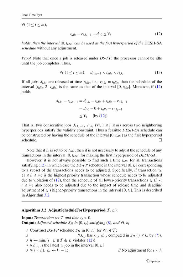
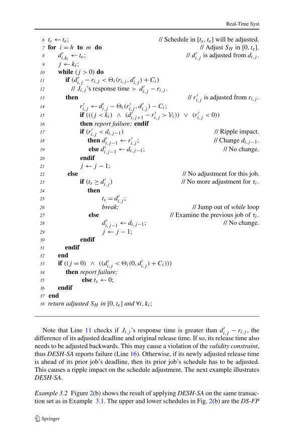
Algorithm 3.2 AdjustScheduleForHyperperiod(T , te):

Input: Transaction set T and time te > 0.Output: Adjusted schedule SH in [0, te] satisfying (8), and ∀i, ki .

1 Construct DS-FP schedule SH in [0, te] for ∀τi ∈ T ;2 //Ji,j has ri,j , di,j computed in SH (j ≤ ki by (7)).3 h ← mini{i | τi ∈ T & τi violates (12)}.4 //Ji,ki

is the latest τi job in the interval [0, te].5 ∀(i < h), ki ← ki − 1; // No adjustment for i < h

Real-Time Syst

6 ts ← te; // Schedule in [ts , te] will be adjusted.7 for i = h to m do // Adjust SH in [0, te].8 d ′

i,ki← te; // d ′

i,j is adjusted from di,j .9 j ← ki ;

10 while (j > 0) do11 if (d ′

i,j − ri,j < �i(ri,j , d′i,j ) + Ci)

12 // Ji,j ’s response time > d ′i,j − ri,j .

13 then // r ′i,j is adjusted from ri,j .

14 r ′i,j ← d ′

i,j − �i(r′i,j , d

′i,j ) − Ci ;

15 if (((j < ki) ∧ (d ′i,j+1 − r ′

i,j > Vi )) ∨ (r ′i,j < 0))

16 then report failure; endif17 if (r ′

i,j < di,j−1) // Ripple impact.18 then d ′

i,j−1 ← r ′i,j ; // Change di,j−1.

19 else d ′i,j−1 ← di,j−1; // No change.

20 endif21 j ← j − 1;22 else // No adjustment for this job.23 if (ts ≥ d ′

i,j ) // No more adjustment for τi .24 then25 ts = d ′

i,j ;26 break; // Jump out of while loop27 else // Examine the previous job of τi .28 d ′

i,j−1 ← di,j−1; // No change.29 j ← j − 1;30 endif31 endif32 end33 if ((j = 0) ∧ ((d ′

i,j < �i(0, d ′i,j ) + Ci)))

34 then report failure;35 else ts ← 0;36 endif37 end38 return adjusted SH in [0, te] and ∀i, ki ;

Note that Line 11 checks if Ji,j ’s response time is greater than d ′i,j − ri,j , the

difference of its adjusted deadline and original release time. If so, its release time alsoneeds to be adjusted backwards. This may cause a violation of the validity constraint,thus DESH-SA reports failure (Line 16). Otherwise, if its newly adjusted release timeis ahead of its prior job’s deadline, then its prior job’s schedule has to be adjusted.This causes a ripple impact on the schedule adjustment. The next example illustratesDESH-SA.

Example 3.2 Figure 2(b) shows the result of applying DESH-SA on the same transac-tion set as in Example 3.1. The upper and lower schedules in Fig. 2(b) are the DS-FP

Real-Time Syst

and its corresponding DESH-SA schedules, respectively. Let te = 33, then h = 3.Only τ3 needs to be adjusted. DESH-SA sets d ′

3,1 = 33. J3,1 can be re-scheduled andits adjusted release time is 27. The newly adjusted schedule from time 0 to 33 is theDESH-SA hyperperiod.

Theorem 3.2 Given a synchronous update transaction set T with known Ci and Vi

(1 ≤ i ≤ m), if (∀i) f mli,0 ≤ Vi

2 in ML, then

WCRTi ≤ f mli,0

where WCRTi and f mli,0 denote the worst-case response time of τi under DS-FP and

ML, respectively.

Proof See Theorem 3.1 in Xiong et al. (2008). �

After the schedule adjustment, the release time and deadline of job Ji,ki+1 (∀i,1 ≤i ≤ m), which appears as the first job in the second hyperperiod, are set as follows:

r ′i,ki+1 = te; (14)

d ′i,ki+1 = te + di,0. (15)

Lemma 3.2 If f mli,0 ≤ Vi

2 in ML, the release time of Ji,kiand the deadline of Ji,ki+1

after adjustment in Algorithm 3.2 is constrained by Vi , i.e.,

d ′i,ki+1 − r ′

i,ki≤ Vi . (16)

Proof ∀i (i < h), (ki − 1) is assigned to ki at Line 5 in Algorithm 3.2. By Theo-rem 3.1,

te + di,0 − ri,ki≤ Vi ⇒

d ′i,ki+1 − r ′

i,ki≤ Vi {by Algorithm 3.2, r ′

i,ki= ri,ki

}Next, we prove it for h ≤ i ≤ m. By schedule adjustment,

r ′i,ki+1 = d ′

i,ki= te. (17)

After the schedule adjustment, according to Theorem 3.2, the following equationshold:

d ′i,ki+1 − r ′

i,ki+1 ≤ f mli,0 ; (18)

d ′i,ki

− r ′i,ki

≤ f mli,0 . (19)

The sum of (18) and (19) is:

d ′i,ki+1 − r ′

i,ki≤ 2f ml

i,0 ≤ Vi .

Thus, (16) holds. �

Real-Time Syst

Lemma 3.2 guarantees that the validity constraint can be satisfied for Ji,kiand

Ji,ki+1, which are two consecutive jobs in different hyperperiods (e.g., the 1st and2nd hyperperiods). Algorithm 3.2 also guarantees that the validity constraint canbe satisfied for jobs Ji,0, . . . , Ji,ki

, which are in the same hyperperiod. Moreover,if the schedule of the first SH hyperperiod can be constructed off-line, the on-linescheduling overhead of DESH-SA in terms of time complexity is constant as it onlyneeds to repeat the schedule of the first SH hyperperiod infinitely. Therefore, thecomplete DESH-SA schedule constructed from Algorithm 3.2 satisfies the aforemen-tioned Properties 3.1 and 3.2.

4 Performance evaluation

This section presents important results from our simulation studies of the DESH algo-rithms. Our goal is to find out whether the DESH algorithms are effective for reduc-ing the DS-FP overhead. The primary performance metrics used in our experimentalstudies are the CPU workload and the number of transactions supported in the system.

4.1 Simulation model and parameters

In the experiments, we investigate whether DESH-SA and DESH-SC can find a hy-perperiod, and if so, how much excess CPU workloads they may incur compared toDS-FP. We also compare the hyperperiod length of DESH-SA and DESH-SC to studythe space efficiency of the approaches, and demonstrate the percentage of transactionsto be adjusted when we calculate the hyperperiod for DESH-SA.

For simplicity, only one version of a real-time data object is maintained. Upon re-freshing a real-time data object, the older version is discarded. We ignore the on-linescheduling overhead in our experiments, and consider it to be O(1) for all algorithms(which is true for DESH algorithms). This is in favor of DS-FP as its schedulingoverhead is ignored for the CPU workload in our experiments. We define Nadjust tobe the average number of jobs whose release times or deadlines are adjusted in [0, te]under DESH-SA.

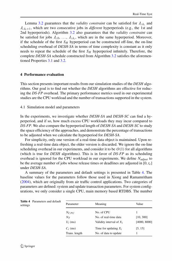
A summary of the parameters and default settings is presented in Table 4. Thebaseline values for the parameters follow those used in Xiong and Ramamritham(2004), which are originally from air traffic control applications. Two categories ofparameters are defined: system and update transaction parameters. For system config-urations, we only consider a single CPU, main memory based RTDBS. The number

Table 4 Parameters and defaultsettings Parameter Meaning Value

NCPU No. of CPU 1

NT No. of real-time data [10, 300]

Vi (ms) Validity interval of Xi [4000, 8000]

Ci (ms) Time for updating Xi [5, 15]

Trans. length No. of data to update 1

Real-Time Syst

of real-time data varies from 10 to 300 and the validity length of each real-time dataobject is uniformly distributed from 4000 to 8000 ms. For update transactions, it isassumed that each transaction updates one real-time data object, and its CPU time isuniformly distributed from 5 to 15 ms.

4.2 Experimental results

In this subsection, the CPU workloads of sensor update transactions produced byDS-FP, DESH-SC and DESH-SA are quantitatively compared. In the first set of ex-periments, update transactions are generated randomly according to the parametersettings in Table 4 while in the second set of experiments,

∑mi=1

Ci

Viof the update

transaction set is fixed at 45% and Vi

Ciis varied to show its impact on the performance

of the algorithms. With the DESH algorithms, the transaction with maximum validityinterval is run at least 200 times (thus issuing 200 jobs) so that the CPU workloadof the first SH hyperperiod is close to UDS . Then the idle times following the com-pletion of those jobs under DS-FP are chosen as te candidates. Those candidates aretested to find out whether the interval [0, te] can be used as the first hyperperiod.

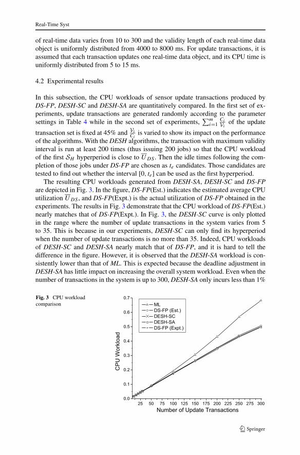
The resulting CPU workloads generated from DESH-SA, DESH-SC and DS-FPare depicted in Fig. 3. In the figure, DS-FP(Est.) indicates the estimated average CPUutilization UDS , and DS-FP(Expt.) is the actual utilization of DS-FP obtained in theexperiments. The results in Fig. 3 demonstrate that the CPU workload of DS-FP(Est.)nearly matches that of DS-FP(Expt.). In Fig. 3, the DESH-SC curve is only plottedin the range where the number of update transactions in the system varies from 5to 35. This is because in our experiments, DESH-SC can only find its hyperperiodwhen the number of update transactions is no more than 35. Indeed, CPU workloadsof DESH-SC and DESH-SA nearly match that of DS-FP, and it is hard to tell thedifference in the figure. However, it is observed that the DESH-SA workload is con-sistently lower than that of ML. This is expected because the deadline adjustment inDESH-SA has little impact on increasing the overall system workload. Even when thenumber of transactions in the system is up to 300, DESH-SA only incurs less than 1%

Fig. 3 CPU workloadcomparison

Real-Time Syst

Fig. 4 Average # of adjustedjobs per transaction in [0, te]

Fig. 5 Average hyperperiodlength comparison

excess CPU workload compared to that of DS-FP. Note that the on-line schedulingoverhead is ignored for DS-FP in our experiments. Thus the actual CPU workloadfor DS-FP should be higher than what is shown in the figure. Also note that the extraoverhead resulting from DESH-SA is adjustable. For example, if the interval [0, te]is further enlarged, the CPU workload of DESH-SA can be reduced, in which case itcan become even closer to that of DS-FP.

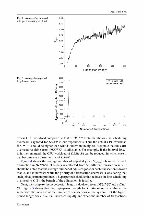
Figure 4 shows the average number of adjusted jobs (Nadjust) obtained for eachtransaction in DESH-SA. The data is collected from 50 different transaction sets. Itshould be noted that the average number of adjusted jobs for each transaction is lowerthan 2, and it increases while the priority of a transaction decreases. Considering thatsuch job adjustment produces a hyperperiod schedule that reduces on-line schedulingoverhead to O(1), the benefit of the adjustment is justified.

Next, we compare the hyperperiod length calculated from DESH-SC and DESH-SA. Figure 5 shows that the hyperperiod length for DESH-SA remains almost thesame with the increase of the number of transactions in the system. But the hyper-period length for DESH-SC increases rapidly and when the number of transactions

Real-Time Syst

Fig. 6 Hyperperiod length vs.Umax (DESH-SC)

Fig. 7 Percentage oftransactions adjusted(DESH-SA)

in the system increases beyond 35, DESH-SC cannot find a hyperperiod. A shorterhyperperiod implies that less space overhead is needed for keeping scheduling infor-mation. This implies that DESH-SA is also space efficient.

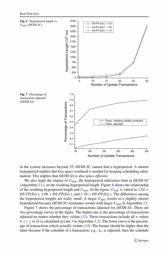
We also study the impact of Umax, the hyperperiod utilization limit in DESH-SC(Algorithm 3.1), on the resulting hyperperiod length. Figure 6 shows the relationshipof the resulting hyperperiod length and Umax. In the figure, Umax is varied as 1.02 ×DS-FP(Est.), 1.06 × DS-FP(Est.), and 1.10 × DS-FP(Est.). The differences amongthe hyperperiod lengths are really small. A larger Umax results in a slightly shorterhyperperiod because DESH-SC terminates sooner with larger Umax in Algorithm 3.1.

Figure 7 shows the percentage of transactions adjusted for DESH-SA. There aretwo percentage curves in the figure. The higher one is the percentage of transactionsadjusted no matter whether they violate (12). Those transactions include all τi whereh ≤ i ≤ m (h is calculated at Line 3 in Algorithm 3.2). The lower curve is the percent-age of transactions which actually violate (12). The former should be higher than thelatter because if the schedule of a transaction, e.g., τh, is adjusted, then the schedule

Real-Time Syst

Fig. 8 CPU workload with

fixed∑m

i=1CiVi

of its lower-priority transactions will be adjusted even if a lower-priority one does notviolate (12) before τh’s adjustment.

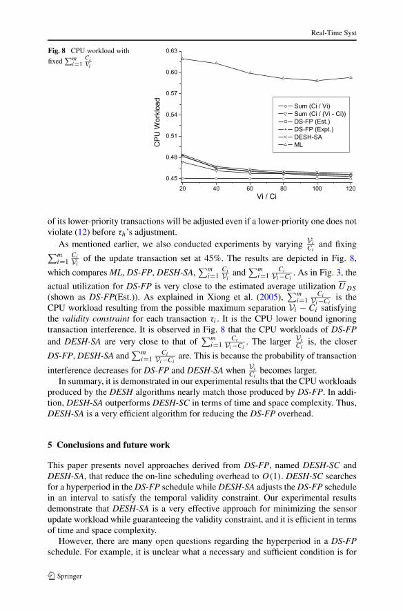
As mentioned earlier, we also conducted experiments by varying Vi

Ciand fixing

∑mi=1

Ci

Viof the update transaction set at 45%. The results are depicted in Fig. 8,

which compares ML, DS-FP, DESH-SA,∑m

i=1Ci

Viand

∑mi=1

Ci

Vi−Ci. As in Fig. 3, the

actual utilization for DS-FP is very close to the estimated average utilization UDS

(shown as DS-FP(Est.)). As explained in Xiong et al. (2005),∑m

i=1Ci

Vi−Ciis the

CPU workload resulting from the possible maximum separation Vi − Ci satisfyingthe validity constraint for each transaction τi . It is the CPU lower bound ignoringtransaction interference. It is observed in Fig. 8 that the CPU workloads of DS-FPand DESH-SA are very close to that of

∑mi=1

Ci

Vi−Ci. The larger Vi

Ciis, the closer

DS-FP, DESH-SA and∑m

i=1Ci

Vi−Ciare. This is because the probability of transaction

interference decreases for DS-FP and DESH-SA when Vi

Cibecomes larger.

In summary, it is demonstrated in our experimental results that the CPU workloadsproduced by the DESH algorithms nearly match those produced by DS-FP. In addi-tion, DESH-SA outperforms DESH-SC in terms of time and space complexity. Thus,DESH-SA is a very efficient algorithm for reducing the DS-FP overhead.

5 Conclusions and future work

This paper presents novel approaches derived from DS-FP, named DESH-SC andDESH-SA, that reduce the on-line scheduling overhead to O(1). DESH-SC searchesfor a hyperperiod in the DS-FP schedule while DESH-SA adjusts the DS-FP schedulein an interval to satisfy the temporal validity constraint. Our experimental resultsdemonstrate that DESH-SA is a very effective approach for minimizing the sensorupdate workload while guaranteeing the validity constraint, and it is efficient in termsof time and space complexity.

However, there are many open questions regarding the hyperperiod in a DS-FPschedule. For example, it is unclear what a necessary and sufficient condition is for

Real-Time Syst

the DESH-SA algorithm to produce a hyperperiod. Also, if a transaction set is notschedulable by DS-FP, is it possible to construct a hyperperiod schedule so that itsconstructed schedule is schedulable? We intend to address these challenging prob-lems in our future work.

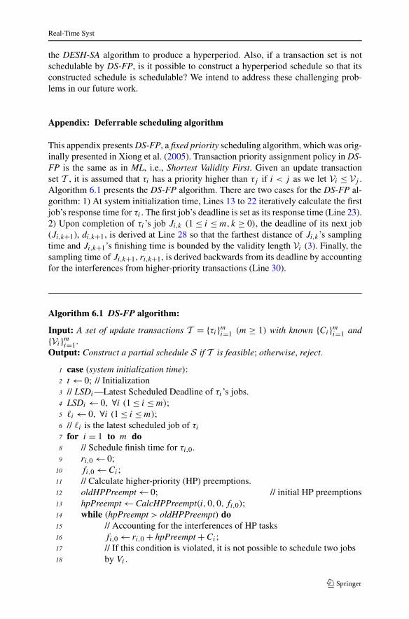
Appendix: Deferrable scheduling algorithm

This appendix presents DS-FP, a fixed priority scheduling algorithm, which was orig-inally presented in Xiong et al. (2005). Transaction priority assignment policy in DS-FP is the same as in ML, i.e., Shortest Validity First. Given an update transactionset T , it is assumed that τi has a priority higher than τj if i < j as we let Vi ≤ Vj .Algorithm 6.1 presents the DS-FP algorithm. There are two cases for the DS-FP al-gorithm: 1) At system initialization time, Lines 13 to 22 iteratively calculate the firstjob’s response time for τi . The first job’s deadline is set as its response time (Line 23).2) Upon completion of τi ’s job Ji,k (1 ≤ i ≤ m,k ≥ 0), the deadline of its next job(Ji,k+1), di,k+1, is derived at Line 28 so that the farthest distance of Ji,k’s samplingtime and Ji,k+1’s finishing time is bounded by the validity length Vi (3). Finally, thesampling time of Ji,k+1, ri,k+1, is derived backwards from its deadline by accountingfor the interferences from higher-priority transactions (Line 30).

Algorithm 6.1 DS-FP algorithm:

Input: A set of update transactions T = {τi}mi=1 (m ≥ 1) with known {Ci}mi=1 and{Vi}mi=1.Output: Construct a partial schedule S if T is feasible; otherwise, reject.

1 case (system initialization time):2 t ← 0; // Initialization3 // LSDi—Latest Scheduled Deadline of τi ’s jobs.4 LSDi ← 0, ∀i (1 ≤ i ≤ m);5 �i ← 0, ∀i (1 ≤ i ≤ m);6 // �i is the latest scheduled job of τi

7 for i = 1 to m do8 // Schedule finish time for τi,0.9 ri,0 ← 0;

10 fi,0 ← Ci ;11 // Calculate higher-priority (HP) preemptions.12 oldHPPreempt ← 0; // initial HP preemptions13 hpPreempt ← CalcHPPreempt(i,0,0, fi,0);14 while (hpPreempt > oldHPPreempt) do15 // Accounting for the interferences of HP tasks16 fi,0 ← ri,0 + hpPreempt + Ci ;17 // If this condition is violated, it is not possible to schedule two jobs18 by Vi .

Real-Time Syst

19 if (fi,0 > Vi − Ci) then abort endif;20 oldHPPreempt ← hpPreempt;21 hpPreempt ← CalcHPPreempt(i,0,0, fi,0);22 end23 di,0 ← fi,0;24 end25 return;26 case (upon completion of Ji,k) :27 // Schedule release time for Ji,k+1.28 di,k+1 ← ri,k + Vi ; // get next deadline for Ji,k+129 // ri,k+1 is also the sampling time for Ji,k+130 ri,k+1 ← ScheduleRT(i, k + 1,Ci, di,k+1);31 return;

Algorithm 6.2 ScheduleRT(i, k, Ci , di,k):

Input: Ji,k with Ci and di,k .Output: ri,k .

1 oldHPPreempt ← 0; // initial HP preemptions2 hpPreempt ← 0;3 ri,k ← di,k − Ci ;4 // Calculate HP preemptions backwards from di,k .5 hpPreempt ← CalcHPPreempt(i, k, ri,k, di,k);6 while (hpPreempt > oldHPPreempt) do7 // Accounting for the interferences of HP tasks8 ri,k ← di,k − hpPreempt − Ci ;9 if (ri,k < di,k−1) then abort endif;

10 oldHPPreempt ← hpPreempt;11 hpPreempt ← GetHPPreempt(i, k, ri,k, di,k);12 end13 return ri,k;

Algorithm 6.3 CalcHPPreempt(i, k, t1, t2):Input: Ji,k , and a time interval [t1, t2).Output: Total cumulative processor demands from higher-priority transactions τj

(1 ≤ j ≤ i − 1) during [t1, t2).1 �i ← k; // Record latest scheduled job of τi .2 di,k ← t2;3 LSDi ← t2;4 if (i = 1)

5 then // No preemptions from higher-priority tasks.6 return 0;7 elsif (LSDi−1 ≥ LSDi )

8 then // Get preemptions from τj (∀j,1 ≤ j < i)

Real-Time Syst

9 // because τj ’s schedule is complete before t2.10 return GetHPPreempt(i, k, t1,LSDi );11 endif12 // build S up to or exceeding t2 for τj (1 ≤ j < i).13 for j = 1 to i − 1 do14 while (dj,�j

< LSDi ) do15 dj,�j +1 ← rj,�j

+ Vj ;16 rj,�j +1 ← ScheduleRT(j, �j + 1,Cj , dj,�j +1);17 �j ← �j + 1;18 LSDj ← dj,�j

;19 end20 end21 return GetHPPreempt(i, k, t1,LSDi );

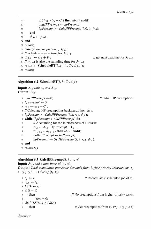
Function ScheduleRT(i, k, Ci, di,k) (Algorithm 6.2) calculates the release timeri,k with known computation time Ci and deadline di,k . It starts with release timeri,k = di,k −Ci , then iteratively calculates �i(ri,k, di,k), the total cumulative proces-sor demands made by all higher-priority jobs of Ji,k during the interval [ri,k, di,k),and adjusts ri,k by accounting for the interferences from higher-priority transactions(Lines 5 to 12). The computation of ri,k continues until the interferences from higher-priority transactions do not change in an iteration. In particular, Line 9 detects any in-feasible schedule. A schedule becomes infeasible under DS-FP if ri,k < di,k−1 (k〉0),i.e., release time of Ji,k becomes earlier than the deadline of its preceding job Ji,k−1.Function GetHPPreempt(i, k, t1, t2) scans the interval [t1, t2), adds up total preemp-tions from τj (∀j, 1 ≤ j ≤ i − 1), and returns �i(t1, t2), the cumulative processordemands of τj during [t1, t2) from schedule S that has been built from CalcHP-Prempt.

Function CalcHPPreempt(i, k, t1, t2) (Algorithm 6.3) calculates �i(t1, t2), thetotal cumulative processor demands made by all higher-priority jobs of Ji,k duringthe interval [t1, t2). Line 7 ensures that (∀j,1 ≤ j < i), τj ’s schedule is completelybuilt before time t2. This is because τi ’s schedule cannot be completely built beforet2 unless the schedules of its higher-priority transactions are complete before t2. Inthis case, the function simply returns an amount of higher-priority preemptions forτi during [t1, t2) by invoking GetHPPreempt(i, k, t1, t2), which returns �i(t1, t2).If any higher-priority transaction τj (j 〈i) does not have a complete schedule during[t1, t2), its schedule S up to or exceeding t2 is built on the fly (Lines 14 to 19).This enables the computation of �i(t1, t2). The latest scheduled deadline of τi ’s job,LSDi , indicates the latest deadline of τi ’s jobs that have been computed.

References

Burns A, Davis R (1996) Choosing task periods to minimise system utilisation in time triggered systems.Inf Process Lett 58:223–229

Chen D, Mok AK (2004) Scheduling similarity-constrained real-time tasks. In: ESA/VLSI, pp 215–221

Real-Time Syst

Chetto H, Chetto M (1989) Some results of the earliest deadline scheduling algorithm. IEEE Trans SoftwEng 15(10):1261–1269

Gerber R, Hong S, Saksena M (1994) Guaranteeing end-to-end timing constraints by calibrating interme-diate processes. In: IEEE real-time systems symposium, December 1994

Gustafsson T, Hansson J (2004a) Data management in real-time systems: a case of on-demand updates invehicle control systems. In: IEEE real-time and embedded technology and applications symposium,pp 182–191

Gustafsson T, Hansson J (2004b) Dynamic on-demand updating of data in real-time database systems. In:ACM SAC

Han CC, Lin KJ, Liu JW-S (1995) Scheduling jobs with temporal distance constraints. SIAM J Comput24(5):1104–1121

Kang KD, Son S, Stankovic JA, Abdelzaher T (2002) A QoS-sensitive approach for timeliness and fresh-ness guarantees in real-time databases. In: EuroMicro real-time systems conference, June 2002

Kuo T, Mok AK (1992) Real-time data semantics and similarity-based concurrency control. In: IEEEreal-time systems symposium, December 1992

Kuo T, Mok AK (1993) SSP: a semantics-based protocol for real-time data access. In: IEEE real-timesystems symposium, December 1993

Ho S, Kuo T, Mok AK (1997) Similarity-based load adjustment for real-time data-intensive applications.In: IEEE real-time systems symposium

Lam KY, Xiong M, Liang B, Guo Y (2004) Statistical quality of service guarantee for temporal consistencyof real-time data objects. In: IEEE real-time systems symposium

Leung J, Whitehead J (1982) On the complexity of fixed-priority scheduling of periodic real-time tasks.Perform Eval 2:237–250

Liu CL, Layland J (1973) Scheduling algorithms for multiprogramming in a hard real-time environment.J ACM 20(1)

Locke D (1997) Real-time databases: real-world requirements. In: Bestavros A, Lin K-J, Son SH (eds)Real-time database systems: issues and applications. Kluwer Academic, Dordrecht, pp 83–91

Ramamritham K (1993) Real-time databases. Distrib Parallel Databases 1(1993):199–226Ramamritham K (1996) Where do time constraints come from and where do they go? Int J Database

Manag 7(2):4–10Song X, Liu JWS (1995) Maintaining temporal consistency: pessimistic vs. optimistic concurrency control.

IEEE Trans Knowl Data Eng 7(5):786–796Xiong M, Ramamritham K (2004) Deriving deadlines and periods for real-time update transactions. IEEE

Trans Comput 53(5):567–583Xiong M, Ramamritham K, Stankovic JA, Towsley D, Sivasankaran RM (2002) Scheduling transactions

with temporal constraints: exploiting data semantics. IEEE Trans Knowl Data Eng 14(5):1155–1166Xiong M, Han S, Lam KY (2005) A deferrable scheduling algorithm for real-time transactions maintaining

data freshness. In: IEEE real-time systems symposiumXiong M, Han S, Chen D (2006) Deferrable scheduling for temporal consistency: schedulability analysis

and overhead reduction. In: IEEE international conference on embedded and real-time computingsystems and applications, August 2006

Xiong M, Han S, Lam KY, Chen D (2008) Deferrable scheduling for maintaining real-time data freshness:algorithm, analysis and results. IEEE Trans Comput 57(7):952–964

Ming Xiong received his Ph.D. degree in Computer Science from Uni-versity of Massachusetts Amherst in 2000. He is currently a memberof technical staff at Bell Labs, Alcatel-Lucent. His research interestsinclude database systems, real-time systems and mobile computing.

Real-Time Syst

Song Han received his Bachelor of Science degree in Computer Sci-ence from Nanjing University, P.R. China in 2003 and Master of Philos-ophy degree in Computer Science from City University of Hong Kongin 2006. He is currently a Ph.D. student in the Department of ComputerSciences at the University of Texas at Austin. His research interests arereal-time systems, database systems, wireless networks and data min-ing. He is a student member of the IEEE.

Deji Chen received his Ph.D. degree in Computer Science from theUniversity of Texas at Austin in 1999. He is currently a senior princi-pal software engineer at Emerson Process Management. His researchinterests include real-time systems and wireless process control.

Kam-Yiu Lam received the B.Sc. (Hons) degree on Computer Stud-ies with distinction and Ph.D. degree from the City University of HongKong in 1990 and 1994, respectively. He is currently an Associate Pro-fessor in the Department of Computer Science, City University of HongKong. His current research interests are real-time database systems,real-time active database systems, mobile computing and distributedmultimedia systems.

Shan Feng received his Ph.D. degree in Computer Software and Theoryfrom Chinese Academy of Science in 2003. He is currently an associateprofessor of Sichuan Normal University, Chengdu, China. His researchinterests include database systems, data mining theories, and real-timesystems.