Embed Size (px)
Citation preview
Real-Time Deferrable Load Control: Handling theUncertainties of Renewable Generation
Lingwen GanCalifornia Inst. of [email protected]
Adam WiermanCalifornia Inst. of Tech.
Ufuk TopcuUniversity of Pennsylvania
[email protected] Chen
California Inst. of [email protected]
Steven H. LowCalifornia Inst. of [email protected]
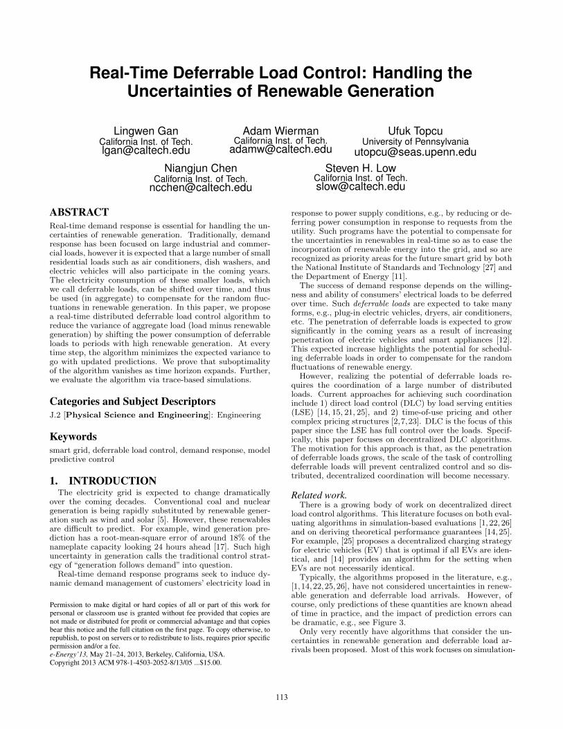
ABSTRACTReal-time demand response is essential for handling the un-certainties of renewable generation. Traditionally, demandresponse has been focused on large industrial and commer-cial loads, however it is expected that a large number of smallresidential loads such as air conditioners, dish washers, andelectric vehicles will also participate in the coming years.The electricity consumption of these smaller loads, whichwe call deferrable loads, can be shifted over time, and thusbe used (in aggregate) to compensate for the random fluc-tuations in renewable generation. In this paper, we proposea real-time distributed deferrable load control algorithm toreduce the variance of aggregate load (load minus renewablegeneration) by shifting the power consumption of deferrableloads to periods with high renewable generation. At everytime step, the algorithm minimizes the expected variance togo with updated predictions. We prove that suboptimalityof the algorithm vanishes as time horizon expands. Further,we evaluate the algorithm via trace-based simulations.
Categories and Subject DescriptorsJ.2 [Physical Science and Engineering]: Engineering
Keywordssmart grid, deferrable load control, demand response, modelpredictive control
1. INTRODUCTIONThe electricity grid is expected to change dramatically
over the coming decades. Conventional coal and nucleargeneration is being rapidly substituted by renewable gener-ation such as wind and solar [5]. However, these renewablesare difficult to predict. For example, wind generation pre-diction has a root-mean-square error of around 18% of thenameplate capacity looking 24 hours ahead [17]. Such highuncertainty in generation calls the traditional control strat-egy of “generation follows demand” into question.
Real-time demand response programs seek to induce dy-namic demand management of customers’ electricity load in
Permission to make digital or hard copies of all or part of this work forpersonal or classroom use is granted without fee provided that copies arenot made or distributed for profit or commercial advantage and that copiesbear this notice and the full citation on the first page. To copy otherwise, torepublish, to post on servers or to redistribute to lists, requires prior specificpermission and/or a fee.e-Energy’13, May 21–24, 2013, Berkeley, California, USA.Copyright 2013 ACM 978-1-4503-2052-8/13/05 ...$15.00.
response to power supply conditions, e.g., by reducing or de-ferring power consumption in response to requests from theutility. Such programs have the potential to compensate forthe uncertainties in renewables in real-time so as to ease theincorporation of renewable energy into the grid, and so arerecognized as priority areas for the future smart grid by boththe National Institute of Standards and Technology [27] andthe Department of Energy [11].
The success of demand response depends on the willing-ness and ability of consumers’ electrical loads to be deferredover time. Such deferrable loads are expected to take manyforms, e.g., plug-in electric vehicles, dryers, air conditioners,etc. The penetration of deferrable loads is expected to growsignificantly in the coming years as a result of increasingpenetration of electric vehicles and smart appliances [12].This expected increase highlights the potential for schedul-ing deferrable loads in order to compensate for the randomfluctuations of renewable energy.
However, realizing the potential of deferrable loads re-quires the coordination of a large number of distributedloads. Current approaches for achieving such coordinationinclude 1) direct load control (DLC) by load serving entities(LSE) [14, 15, 21, 25], and 2) time-of-use pricing and othercomplex pricing structures [2,7,23]. DLC is the focus of thispaper since the LSE has full control over the loads. Specif-ically, this paper focuses on decentralized DLC algorithms.The motivation for this approach is that, as the penetrationof deferrable loads grows, the scale of the task of controllingdeferrable loads will prevent centralized control and so dis-tributed, decentralized coordination will become necessary.
Related work.There is a growing body of work on decentralized direct
load control algorithms. This literature focuses on both eval-uating algorithms in simulation-based evaluations [1, 22, 26]and on deriving theoretical performance guarantees [14,25].For example, [25] proposes a decentralized charging strategyfor electric vehicles (EV) that is optimal if all EVs are iden-tical, and [14] provides an algorithm for the setting whenEVs are not necessarily identical.
Typically, the algorithms proposed in the literature, e.g.,[1,14,22,25,26], have not considered uncertainties in renew-able generation and deferrable load arrivals. However, ofcourse, only predictions of these quantities are known aheadof time in practice, and the impact of prediction errors canbe dramatic, e.g., see Figure 3.
Only very recently have algorithms that consider the un-certainties in renewable generation and deferrable load ar-rivals been proposed. Most of this work focuses on simulation-
113
based studies, e.g., [6,9,10]; however some work does deriveanalytic performance guarantees [4, 8, 24, 29]. For example,reference [8] proposes an algorithm that achieves the optimalcompetitive ratio in the case where renewable generation isprecisely known (and constant) and [24] proposes an algo-rithm with some worst-case performance guarantees. Notethat, while the algorithms proposed in [8, 24] are analyzedwith a “worst-case” perspective, this paper focuses on the“average-case” perspective.
Summary and contributions.The goal of this paper is to provide a real-time
algorithm for decentralized deferrable load controlin the context of uncertain predictions about bothfuture loads and future renewable generation. Morespecifically, in this paper we propose a novel extension ofthe“optimal deferrable load control problem”studied in [14].This extension incorporates uncertainty about both deferrableand non-deferrable loads, in addition to inexact predictionsof renewable generation; and then uses this problem to de-rive a new algorithm for deferrable load control. Further, weperform both analytic and trace-based performance analysisof the algorithm in order to quantify the impact of predic-tion uncertainties on deferrable load control. In particular,the contributions of the work are threefold.
First, we model renewable generation prediction as a Wienerfiltering process [31] (Section 2), that is able to model anyzero mean, stationary prediction evolutions. Additionally,the formulation includes a very general model for deferableloads that allows for heterogeneous deadlines and maximumcharging rates, as well as stochastic arrivals.
Second, in the context of this model, we introduce a real-time algorithm for deferrable load control with uncertainty(Section 3.2). The real-time algorithm essentially solves aseries of optimal control problems whose horizon lengthsshrink with time. At any time, the algorithm uses onlythe information that is available, i.e., specifications of de-ferrable loads that have already arrived and predictions onfuture loads and renewable generation. In this sense, thealgorithm we propose is a (non-trivial) extension of the al-gorithm proposed in [14], which applies only in the case ofexact knowledge of loads and renewables. A key techniqueintroduced by the algorithm is the concept of a “pseudo de-ferrable load,” which is simulated at the utility to representfuture deferrable load arrivals.
Third, we perform a detailed performance analysis of ourproposed algorithm. The performance analysis uses both an-alytic results and trace-based experiments to study (i) thereduction in expected load variance achieved via deferrableload control, and (ii) the value of using real-time control viaour algorithm when compared with static (open-loop) con-trol. The theorems in Section 4 characterize the impact ofprediction inaccuracy on deferrable load control. These ana-lytic results highlight that as the time horizon expands, theexpected load variance obtained by our proposed algorithmapproaches the optimal value (Corollary 3). Also, as thetime horizon expands, the algorithm obtains an increasingvariance reduction over the optimal static algorithm (Corol-lary 5, 6). Furthermore, in Section 5 we provide trace-basedexperiments using data from Southern California Edison andAlberta Electric System Operator to validate the analyticresults. These experiments highlight that our proposed al-gorithm obtains a small suboptimality under high uncertain-ties of renewable generation, and has significant performanceimprovement over the optimal static control.
2. MODEL OVERVIEW AND NOTATIONThis paper studies the design and analysis of real-time
control algorithms for scheduling deferrable loads to com-pensate for the random fluctuations in renewable generation.In the following we present a model of this scenario thatserves as the basis for our algorithm design and performanceevaluation. The model includes renewable generation, non-deferrable loads, and deferrable loads, which are described inturn. The key differentiation of this model from that of [14]is the inclusion of uncertainties (prediction errors) on futurerenewable generation and loads.
Throughout, we consider a discrete-time model over a fi-nite time horizon. The time horizon is divided into T timeslots of equal length and labeled 1, . . . , T . In practice, thetime horizon could be one day and the length of a time slotcould be 10 minutes.
2.1 Renewable generation andnon-deferrable load
Renewable generation like wind is stochastic and difficultto predict. Similarly, non-deferrable load including lights arehard to predict at a low aggregation level.
Since the focus is on scheduling deferrable loads, we ag-gregate renewable generation and non-deferrable load intoone process termed the base load, b = {b(τ)}Tτ=1, which isdefined as the difference between non-deferrable load andrenewable generation, and is a stochastic process.
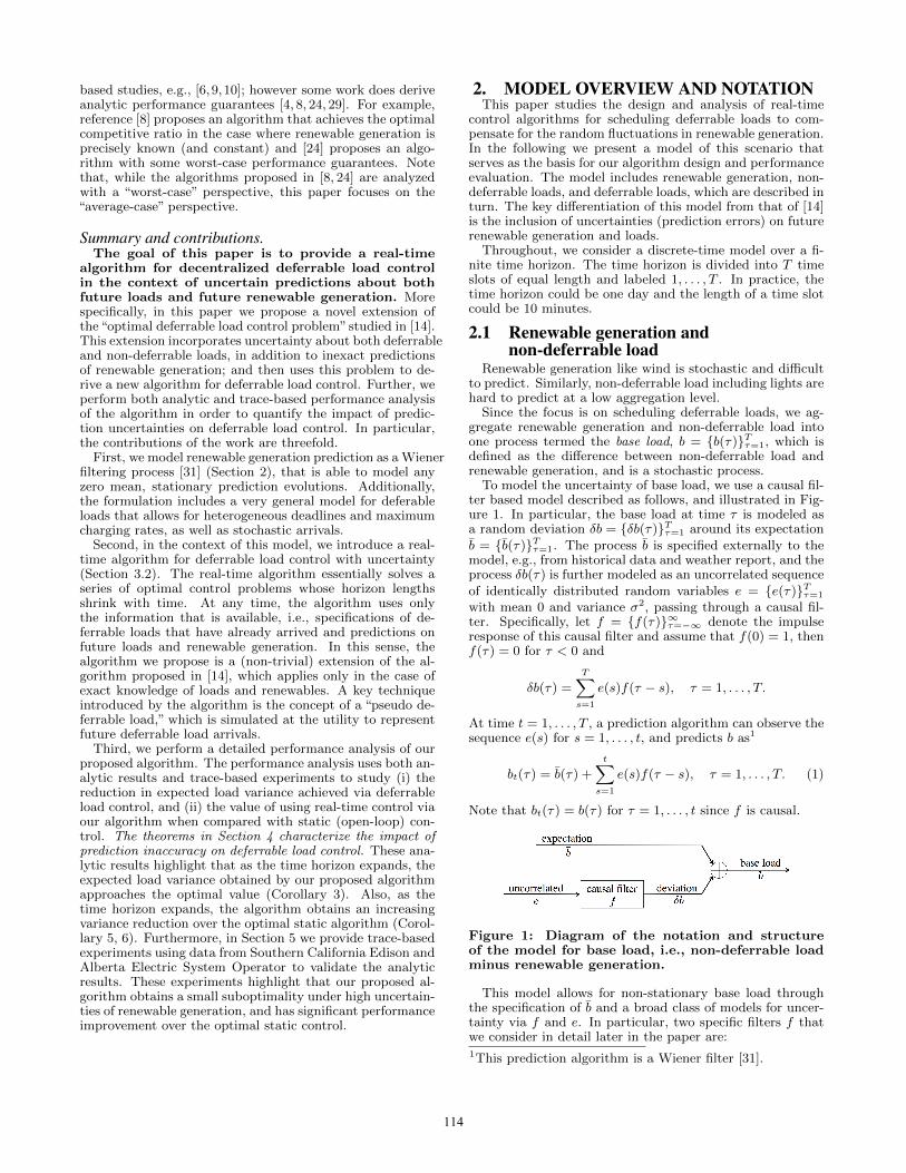
To model the uncertainty of base load, we use a causal fil-ter based model described as follows, and illustrated in Fig-ure 1. In particular, the base load at time τ is modeled asa random deviation δb = {δb(τ)}Tτ=1 around its expectationb̄ = {b̄(τ)}Tτ=1. The process b̄ is specified externally to themodel, e.g., from historical data and weather report, and theprocess δb(τ) is further modeled as an uncorrelated sequenceof identically distributed random variables e = {e(τ)}Tτ=1
with mean 0 and variance σ2, passing through a causal fil-ter. Specifically, let f = {f(τ)}∞τ=−∞ denote the impulseresponse of this causal filter and assume that f(0) = 1, thenf(τ) = 0 for τ < 0 and
δb(τ) =
T∑s=1
e(s)f(τ − s), τ = 1, . . . , T.
At time t = 1, . . . , T , a prediction algorithm can observe thesequence e(s) for s = 1, . . . , t, and predicts b as1
bt(τ) = b̄(τ) +
t∑s=1
e(s)f(τ − s), τ = 1, . . . , T. (1)
Note that bt(τ) = b(τ) for τ = 1, . . . , t since f is causal.
Figure 1: Diagram of the notation and structureof the model for base load, i.e., non-deferrable loadminus renewable generation.
This model allows for non-stationary base load throughthe specification of b̄ and a broad class of models for uncer-tainty via f and e. In particular, two specific filters f thatwe consider in detail later in the paper are:1This prediction algorithm is a Wiener filter [31].
114
(i) A filter with finite but flat impulse response, i.e., thereexists ∆ > 0 such that
f(t) =
{1 if 0 ≤ t < ∆
0 otherwise;
(ii) A filter with an infinite and exponentially decaying im-pulse response, i.e., there exists a ∈ (0, 1) such that
f(t) =
{at if t ≥ 0
0 otherwise.
These two filters provide simple but informative examplesfor our discussion in Section 4.
2.2 Deferrable loadTo model deferrable loads we consider a setting where N
deferrable loads arrive over the time horizon, each requiringa certain amount of electricity by a given deadline. Further,a real-time algorithm has imperfect information about thearrival times and sizes of these deferrable loads.
More specifically, we assume a total of N deferrable loadsand label them in increasing order of their arrival times by1, . . . , N , i.e., load n arrives no later than load n + 1 forn = 1, . . . , N − 1. Further, we define N(t) as the number ofloads that arrive before (or at) time t for t = 1, . . . , T and fixN(0) := 0. Thus, load 1, . . . , N(t) arrive before or at time tfor t = 1, . . . , T and N(T ) = N .
For each deferrable load, its arrival time and deadline,as well as other constraints on its power consumption, arecaptured via upper and lower bounds on its possible powerconsumption during each time. Specifically, the power con-sumption of deferrable load n at time t, pn(t), must be be-tween given lower and upper bounds p
n(t) and pn(t), i.e.,
pn(t) ≤ pn(t) ≤ pn(t), n = 1, . . . , N, t = 1, . . . , T. (2)
These are specified externally to the model. For example, ifan electric vehicle plugs in with Level II charging, then itspower consumption must be within [0, 3.3]kW. However, ifit is not plugged in (has either not arrived yet or has alreadydeparted) then its power consumption is 0kW, i.e., within[0, 0]kW. Further, we assume that a deferrable load n mustwithdraw a fixed amount of energy Pn by its deadline, i.e.,
T∑t=1
pn(t) = Pn, n = 1, . . . , N. (3)
Finally, the N deferrable loads arrive randomly through-out the time horizon. Define
a(t) :=
N(t)∑n=N(t−1)+1
Pn (4)
as the total energy request of all deferrable loads that arriveat time t for t = 1, . . . , T . We assume that {a(t)}Tt=1 isa sequence of independent identically distributed randomvariables with mean λ and variance s2. Further, define
A(t) :=
T∑τ=t+1
a(τ) (5)
as the total energy requested after time t for t = 1, . . . , T .In summary, at time t = 1, . . . , T , a real-time algorithm
has full information about the deferrable loads that have ar-rived, i.e., p
n, pn, and Pn for n = 1, . . . , N(t), and knows
the expectation of future deferrable load total energy re-quest E(A(t)). However, a real-time algorithm has no otherknowledge about deferrable loads that arrive after time t.
2.3 The deferrable load control problemWe can now formally state the deferrable load control
problem that is the focus of this paper. Recall that theobjective of real-time deferrable load control is to compen-sate for the random fluctuations in renewable generation andnon-deferrable load in order to “flatten” the aggregate loadd = {d(t)}Tt=1, which is defined as
d(t) = b(t) +
N∑n=1
pn(t), t = 1, . . . , T. (6)
In this paper, we focus on minimizing the sample path vari-ance of the aggregate load d, V (d), as a measure of“flatness”,that is defined as
V (d) =1
T
T∑t=1
(d(t)− 1
T
T∑τ=1
d(τ)
)2
. (7)
We can now formally specify the optimal deferrable loadcontrol (ODLC) problem that we seek to solve:
ODLC: min1
T
T∑t=1
(d(t)− 1
T
T∑τ=1
d(τ)
)2
(8)
over pn(t), d(t), ∀n, t
s.t. d(t) = b(t) +
N∑n=1
pn(t), ∀t;
pn(t) ≤ pn(t) ≤ pn(t), ∀n, t;
T∑t=1
pn(t) = Pn, ∀n.
In the above ODLC, the objective is simply the samplepath variance of the aggregate load, V (d), and the con-straints correspond to equations (6), (2), and (3), respec-tively. We chose V (d) as the objective for ODLC becauseof its significance for microgrid operators [20]. However, ad-ditionally, [14] has proven that the optimal solution doesnot change if the objective function V (d) is replaced by
f(d) =∑Tt=1 U(d(t)) where U : R → R is strictly convex.
Hence, we can use V (d) without loss of generality.
3. ALGORITHM DESIGNGiven the optimal deferrable load control (ODLC) prob-
lem defined in (8), the first contribution of this paper is todesign an algorithm that solves ODLC in real-time, givenuncertain predictions of base and deferrable loads.
There are two key challenges for the algorithm design.First, the algorithm has access only to uncertain predictionsat any given time, i.e., at time t the algorithm only knowsdeferrable loads 1 to N(t) rather than 1 to N , and onlyknows the prediction bt instead of b itself. Second, even ifthere was no uncertainty in predictions, solving the ODLCproblem requires significant computational effort when thereare a large number of deferrable loads.
Motivated by these challenges, in this section we designa decentralized algorithm with strong performance guaran-tees even when there is uncertainty in the predictions. Thealgorithm builds on the work of [14], which provides a decen-tralized algorithm for the case without uncertainty in pre-dictions. We present the details of the algorithm from [14] inSection 3.1 and then present a modification of the algorithmto handle uncertain predictions in Section 3.2.
115
Algorithm 1 Deferrable load control without uncertainty
Input: The utility knows the base load b and the numberN of deferrable loads. Each load n ∈ {1, . . . , N} knowsits energy request Pn and power consumption bounds pnand p
n. The utility sets K, the number of iterations.
Output: Deferrable load schedule p = (p1, . . . , pN ).
(i) Set k ← 0 and intitialize the schedule p(k) as
p(k)n (t)← 0, t = 1, . . . , T , n = 1, . . . , N .
(ii) The utility calculates the average load g(k) = d(k)/N ,
g(k)(t)← 1
N
(b(t) +
N∑n=1
p(k)n (t)
), t = 1, . . . , T,
and broadcasts g(k) to all deferrable loads.
(iii) Each load n updates a new schedule p(k+1)n by solving
min
T∑τ=1
g(k)(τ)pn(τ) +1
2
(pn(τ)− p(k)n (τ)
)2over pn(1), . . . , pn(T )
s.t. pn(τ) ≤ pn(τ) ≤ pn(τ), ∀τ ;
T∑τ=1
pn(τ) = Pn,
and reports p(k+1)n to the utility.
(iv) Set k ← k + 1. If k < K, go to Step (ii).
3.1 Load control without uncertaintyWe start with the case where the algorithm has complete
knowledge (no uncertainty) about base load and deferrableloads. In this context, the key algorithmic challenge is tosolve the ODLC problem in (8) via a decentralized algo-rithm. Such a decentralized algorithm was proposed in [14],and we summarize the algorithm and its analysis here.
Algorithm definition: The algorithm from [14] is givenin Algorithm 1. It is iterative and the superscripts in brack-ets denote the round of iteration. In each iteration k ≥ 0,there are two key steps: Step (ii) and (iii). In Step (ii), the
utility calculates the average load g(k) and broadcasts it toall deferrable loads. Note that the utility only needs to know
the reported schedule p(k)n , the base load b, and the number
of deferrable loads N . It does not need to know the con-straints of the deferable loads. In Step (iii), each deferrable
load n updates p(k+1)n by solving a convex optimization. The
objective function has two terms. The first term can be in-terpreted as the electricity bill if the electricity price was setto g(k). The second term vanishes as iterations continue.
Algorithm convergence results: Importantly, thoughAlgorithm 1 is iterative, it converges very fast. In fact, thesimulations in [14] stop the iterations after 15 rounds (i.e.,K=15) in all cases because convergence is already achieved.Further, Algorithm 1 provably solves the ODLC problemgiven in (8) when there is no uncertainty, i.e., when N(t) =N and bt = b for t = 1, . . . , T [14]. More precisely, letO denote the set of optimal solutions to (8), and defined(p,O) := minp̂∈O ‖p− p̂‖ as the distance from a deferrableload schedule p to optimal deferrable load schedules O.
Proposition 1 ( [14]). When there is no uncertainty,i.e., N(t) = N and bt = b for t = 1, . . . , T , the deferrable
load schedules p(k) obtained by Algorithm 1 converge to op-timal schedules to ODLC, i.e., d(p(k),O)→ 0 as k →∞.
A particular class of optimal solutions will be of interest
to us later in the paper, so we define them here. Specifically,we call a feasible deferrable load schedule p = (p1, . . . , pN )valley-filling, if there exists some constant C ∈ R such that∑Nn=1 pn(t) = (C − b(t))+ for t = 1, . . . , T .
Proposition 2 ( [14]). If a valley-filling deferrable loadschedule exists, then it solves ODLC. Further, in such cases,all optimal schedules to ODLC have the same aggregate load.
Note that valley-filling schedules tend to exist if there isa large number of deferrable loads, in such settings optimalsolutions to ODLC are valley-filling.
3.2 Load control with uncertaintyAlgorithm 1 provides a decentralized approach for solving
the ODLC problem; however it assumes exact knowledge(certainty) about base load and deferrable loads. In thissection, we adapt Algorithm 1 to the setting where thereis uncertainty in base load and deferrable load predictions,while maintaining strong performance guarantees. In par-ticular, in this section we assume that at time t, only theprediction bt is known, not b itself, and only informationabout deferrable loads 1 to N(t) and the expectation of fu-ture energy requests E(A(t)) are known.
Algorithm definition: To adapt Algorithm 1 to dealwith uncertainty, the first step is straightforward. In partic-ular, it is natural to replace the base load b by its predictionbt in Algorithm 1 to deal with the unavailability of b.
However, dealing with unavailable future deferrable loadinformation is trickier. To do this we use a pseudo deferrableload, which is simulated at the utility, to represent futuredeferrable loads. More specifically, let q = {q(τ)}Tτ=t withq(t) = 0 denote the power consumption of the pseudo load,and assume that it requests E(A(t)) amount of energy, i.e.,
T∑τ=t
q(τ) = E(A(t)). (9)
We also assume that q is point-wise upper and lower boundedby some upper and lower bounds q and q, i.e.,
q(τ) ≤ q(τ) ≤ q(τ), τ = t, . . . , T. (10)
Note that q(t) = q(t) = 0. The bounds q and q should be setaccording to historical data. Here, for simplicity, we considerthem to be q(τ) = 0 and q(τ) =∞ for τ = t+ 1, . . . , T .
Given the above setup, the utility solves the followingproblem at every time slot t = 1, . . . , T , to accommodatethe availability of only partial information.
ODLC-t: min
T∑τ=t
(d(τ)− 1
T − t+ 1
T∑s=t
d(s)
)2
(11)
over pn(τ), q(τ), d(τ), n ≤ N(t), τ ≥ t
s.t. d(τ) = bt(τ) +
N(t)∑n=1
pn(τ) + q(τ), τ ≥ t;
pn(τ) ≤ pn(τ) ≤ pn(τ), n ≤ N(t), τ ≥ t;
T∑τ=t
pn(τ) = Pn(t), n ≤ N(t);
q(τ) ≤ q(τ) ≤ q(τ), τ ≥ t;T∑τ=t
q(τ) = E(A(t))
where Pn(t) = Pn−∑t−1τ=1 pn(τ) is the energy to be consumed
at or after time t, for n = 1, . . . , N(t) and t = 1, . . . , T .
116
Algorithm 2 Deferrable load control with uncertainty
Input: At time t, the utility knows the prediction bt of baseload and the number N(t) of deferrable loads. Each de-ferrable load n ∈ {1, . . . , N(t)} knows its future energyrequest Pn(t) and power consumption bounds pn and p
n.
The utility sets K, the number iterations.Output: At time t, output the power consumption pn(t)
for deferrable loads 1, . . . , N(t).
At time slot t = 1, . . . , T :
(i) Set k ← 0. Each deferrable load n ∈ {1, . . . , N(t)}initializes its schedule {p(0)n (τ)}Tτ=t as
p(0)n (τ)←
{p(K)n (τ) if n ≤ N(t− 1)
0 if n > N(t− 1), τ = t, . . . , T
where p(K)n is the schedule of load n in iteration K of
the previous time slot t− 1.
(ii) The utility solves
min
T∑τ=t
bt(τ) +
N(t)∑n=1
p(k)n (τ) + q(τ)
2
over q(t), . . . , q(T )
s.t. q(τ) ≤ q(τ) ≤ q(τ), τ ≥ t;T∑τ=t
q(τ) = E(A(t))
to obtain a pseudo schedule {q(k)(τ)}Tτ=t. The util-ity then calculates the average aggregate load per de-ferrable load g(k) as
g(k)(τ)← 1
N(t)
bt(τ) +
N(t)∑n=1
p(k)n (τ) + q(k)(τ)
for τ = t, . . . , T, and broadcasts {g(k)(τ)}Tτ=t to de-ferrable loads n = 1, . . . , N(t).
(iii) Each deferrable load n = 1, . . . , N(t) solves
min
T∑τ=t
g(k)(τ)pn(τ) +1
2
(pn(τ)− p(k)n (τ)
)2over pn(t), . . . , pn(T )
s.t. pn(τ) ≤ pn(τ) ≤ pn(τ), τ ≥ t;
T∑τ=t
pn(τ) = Pn(t),
to obtain a new schedule {p(k+1)n (τ)}Tτ=t, and reports
{pk+1n (τ)}Tτ=t to the utility.
(iv) Set k ← k + 1. If k < K, go to Step (ii).
(v) Deferrable load n ∈ {1, . . . , N(t)} sets pn(t) ← pKn (t)and Pn(t+ 1)← Pn(t)− pn(t).
Now, adjusting Algorithm 1 to solve ODLC-t gives Algo-rithm 2, which is real-time and shrinking-horizon. Note thatif base load prediction is exact (i.e., bt = b for t = 1, . . . , T )and all deferrable loads arrive at the beginning of the timehorizon (i.e., N(t) = N for t = 1, . . . , T ), then ODLC-1reduces to ODLC and Algorithm 2 reduces to Algorithm 1.
Algorithm convergence results: We provide analyticguarantees on the convergence and optimality of Algorithm2. In particular, we prove that Algorithm 2 solves ODLC-
t at every time slot t. Specifically, let O(t) denote the setof optimal schedules to ODLC-t, and define d(p,O(t)) :=min(p̂,q̂)∈O(t) ‖p − p̂‖ as the distance from a schedule p tooptimal schedules O(t) at time t, for t = 1, . . . , T .
Theorem 1. At time t = 1, . . . , T , the deferrable loadschedules p(k) obtained by Algorithm 2 converge to optimalschedules to ODLC-t, i.e., d(p(k),O(t))→ 0 as k →∞.
The theorem is proved in Appendix A.1. Though iterative,Algorithm 2 converges fast, similar to Algorithm 1. In thesimulations, setting K = 15 is enough for all test cases.
Similar to Proposition 2,“t-valley-filling”provides a simplecharacterization of the solutions to ODLC-t. Specifically, attime t = 1, . . . , T , a feasible schedule (p, q) is called t-valley-filling, if there exists some constant C(t) ∈ R such that
q(τ) +
N(t)∑n=1
pn(τ) = (C(t)− bt(τ))+, τ = t, . . . , T. (12)
Given this definition of t-valley-filling, the following corollaryfollows immediately from Proposition 2.
Corollary 1. At time t = 1, . . . , T , a t-valley-filling de-ferrable load schedule, if exists, solves ODLC-t. Further-more, in such cases, all optimal schedules to ODLC-t havethe same aggregate load.
This corollary serves as the basis for the performance anal-ysis we perform in Section 4. Remember that t-valley-fillingschedules tend to exist in cases where there are a large num-bers of deferrable loads.
4. PERFORMANCE EVALUATIONTo this point, we have shown that Algorithm 2 makes “op-
timal” decisions with the information available at every timeslot, i.e., it solves ODLC-t at time t for t = 1, . . . , T . How-ever, these decisions are still suboptimal compared to whatcould be achieved if exact information was available. In thissection, our goal is to understand the impact of uncertaintyon the performance. In particular, we study two questions:
(i) How do the uncertainties about base load and deferrableloads impact the expected sample path load varianceobtained by Algorithm 2?
(ii) What is the improvement of using the real-time controlprovided by Algorithm 2 over using the optimal staticcontrol?
Our answers to these questions are below. Throughout,we focus on the special, but practically relevant, case whena t-valley-filling schedule exists at every time t = 1, . . . , T .As we have mentioned previously, when the number of de-ferrable loads is large this is a natural assumption that holdsfor practical load profiles. The reason for making this as-sumption is that it allows us to use the characterization ofoptimal schedules given in (12). In fact, without loss of gen-erality, we further assume C(t) ≥ bt(τ) for τ = t, . . . , T ,under which (12) implies
d(t) = C(t) =1
T − t+ 1
T∑τ=t
bt(τ) + E(A(t)) +
N(t)∑n=1
Pn(t)
(13)
for t = 1, . . . , T . Thus, equation (13) defines the model weuse for the performance analysis of Algorithm 2.
117
The expected load variance of Algorithm 2.We start by calculating the expected load variance, E(V ),
of Algorithm 2. The goal is to understand how uncertaintyabout base load and deferrable loads impacts the load vari-ance. Note that, if there are no base load prediction errorsand deferrable loads arrive at the beginning of the time hori-zon, then Algorithm 2 obtains optimal schedules that havezero load variance. In contrast, when there are base loadprediction errors and stochastic deferrable load arrivals, theexpected load variance is given by the following theorem.
To state the result, recall that {f(t)}∞t=−∞ is the causalfilter modeling the correlation of base load and define F (t) :=∑ts=0 f(s) for t = 0, . . . , T .
Theorem 2. The expected load variance E(V ) obtainedby Algorithm 2 is
E(V ) =s2
T
T∑t=2
1
t+σ2
T 2
T−1∑t=0
F 2(t)T − t− 1
t+ 1. (14)
The theorem is proved in Appendix A.4.Theorem 2 explicitly states the interaction of the variabil-
ity of base load prediction (σ) and deferrable load predic-tion (s) with the horizon length T . Besides, it highlights thecorrelation of base load prediction error through F . Morespecifically, the expected load variance E(V ) tends to 0 asthe uncertainties in base load and deferrable loads vanish,i.e., σ → 0 and s→ 0.
Corollary 2. The expected load variance E(V ) → 0 asσ → 0 and s→ 0.
Another remark about Theorem 2 is that the two termsin (14) correspond to the impact of the uncertainties in de-ferrable loads and base load respectively. In particular, The-orem 2 is proved in Section A.4 by analyzing these two casesseparately and then combining the results. Specifically, thefollowing two lemmas are the key pieces in the proof of The-orem 2, but are also of interest in their own right.
Lemma 1. If there is no base load prediction error, i.e.,bt = b for t = 1, . . . , T , then the expected load variance ob-tained by Algorithm 2 is
E(V ) = s2∑Tt=2
1t
T≈ s2 lnT
T.
The lemma is proved in Appendix A.2.
Lemma 2. If there are no deferrable load arrivals aftertime 1, i.e., N(t) = N for t = 1, . . . , T , then the expectedload variance obtained by Algorithm 2 is
E(V ) =σ2
T 2
T−1∑t=0
F 2(t)T − t− 1
t+ 1.
The lemma is proved in Appendix A.3.Lemma 1 highlights that the more uncertainty in deferrable
load arrival, i.e., the larger s, the larger the expected loadvariance E(V ). On the other hand, the longer the time hori-zon T , the smaller the expected load variance E(V ).
Similarly, Lemma 2 highlights that a larger base load pre-diction error, i.e., a larger σ, results in a larger expected loadvariance E(V ). However, if the impulse response {f(t)}∞t=−∞of the modeling filter of the base load decays fast enoughwith t, then the following corollary highlights that the ex-pected load variance actually tends to 0 as time horizon Tincreases despite the uncertainty of base load predictions.
Corollary 3. If there are no deferrable load arrivals af-ter time 1, i.e., N(t) = N for t = 1, . . . , T , and |f(t)| ∼O(t−1/2−α) for some α > 0, then the expected load varianceobtained by Algorithm 2 satisfies E(V )→ 0 as T →∞.
The corollary is proved in Appendix A.5.
The improvement of Algorithm 2 over static control.The goal of this section is to quantify the improvement
of real-time control via Algorithm 2 over the optimal static(open-loop) control. To be more specific, we compare theexpected load variance E(V ) obtained by the real-time con-trol Algorithm 2, with the expected load variance E(V ′)obtained by the optimal static control, which only uses baseload prediction at the beginning of the time horizon (i.e., b̄)to compute deferrable load schedules. We assume N(t) = Nfor t = 1, . . . , T in this section since otherwise any static con-trol cannot obtain a schedule for all deferrable loads. Thus,the interpretation of the results that follow is as a quan-tification of the value of incorporating updated base loadpredictions into the deferrable load controller.
To begin the analysis, note that E(V ) for this setting isgiven in Lemma 2. Further, it can be verified that the op-timal static control is to solve ODLC with b replaced by b̄,and the corresponding expected load variance E(V ′) is givenby the following lemma.
Lemma 3. If there is no stochastic load arrival, i.e., N(t) =N for t = 1, . . . , T , then the expected load variance E(V ′)obtained by the optimal static control is
E(V ′) =σ2
T 2
T−1∑t=0
(T (T − t)f2(t)− F 2(t)
).
The lemma is proved in Appendix A.6.Next, comparing E(V ) and E(V ′) given in Lemma 2 and
3 shows that Algorithm 2 always obtains a smaller expectedload variance than the optimal static control. Specifically,
Corollary 4. If there is no deferrable load arrival aftertime 1, i.e., N(t) = N for t = 1, . . . , T , then
E(V ′)−E(V ) =σ2
T
T∑t=1
1
2t
t−1∑m=0
t−1∑n=0
(f(m)− f(n))2 ≥ 0.
The corollary is proved in the extended version [16].Corollary 4 highlights that Algorithm 2 is guaranteed to
obtain a smaller expected load variance than the optimalstatic control. The next step is to quantify how much smallerE(V ) is in comparison with E(V ′).
To do this we compute the ratio E(V ′)/E(V ). Unfortu-nately, the general expression for the ratio is too complexto provide insight, so we consider two representative casesfor the impulse response f(t) of the causal filter in order toobtain insights. Specifically, we consider examples (i) and(ii) from Section 2.1. Briefly, in (i) f(t) is finite and in (ii)f(t) is infinite but decays exponentially in t. For these twocases, the ratio E(V ′)/E(V ) is summarized in the followingcorollaries.
Corollary 5. If there is no deferrable load arrival aftertime 1, i.e., N(t) = N for t = 1, . . . , T , and there exists∆ > 0 such that
f(t) =
{1 if 0 ≤ t < ∆
0 otherwise,
then
E(V ′)
E(V )=
T/∆
ln(T/∆)
(1 +O
(1
ln(T/∆)
)).
The corollary is proved in the extended version [16].
Corollary 6. If there is no deferrable load arrival aftertime 1, i.e., N(t) = N for t = 1, . . . , T , and there existsa ∈ (0, 1) such that
f(t) =
{at if t ≥ 0
0 otherwise,
118
then
E(V ′)
E(V )=
1− a1 + a
T
lnT
(1 +O
(ln lnT
lnT
)).
The corollary is proved in the extended version [16].Corollary 5 highlights that, in the case where f is finite,
if we define λ = T/∆ as the ratio of time horizon to filterlength, then the load reduction roughly scales as λ/ ln(λ).Thus, the longer the time horizon is in comparison to thefilter length, the larger expected load variance reduction weobtain from using Algorithm 2 as compared with the optimalstatic control.
Similarly, Corollary 6 highlights that, in the case wheref is infinite and exponentially decaying, the expected loadvariance reduction scales with T as T/ lnT with coefficient(1−a)/(1+a). Thus, the smaller a is, which means the fasterf dies out, the more load variance reduction we obtain byusing real-time control. This is similar to having a smaller∆ in the previous case.
5. EXPERIMENTAL RESULTSIn this section we use trace-based experiments to explore
the generality of the analytic results in the previous sec-tion. In particular, the results in the previous section char-acterize the expected load variance obtained by Algorithm2 as a function of prediction uncertainties, and quantify theimprovement of Algorithm 2 over the optimal static (open-loop) controller. However, the analytic results make simpli-fying assumptions on the form of uncertainties and solutionschedules (equation (13)). Therefore, it is important to as-sess the performance of the algorithm using real-world data.
5.1 Experimental setupThe numerical experiments we perform use a time horizon
of 24 hours, from 20:00 to 20:00 on the following day. Thetime slot length is 10 minutes, which is the granularity ofthe data we have obtained about renewable generation.
Base load.Recall that base load is a combination of non-deferrable
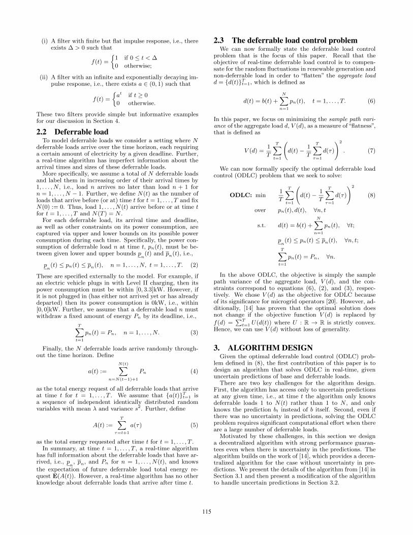
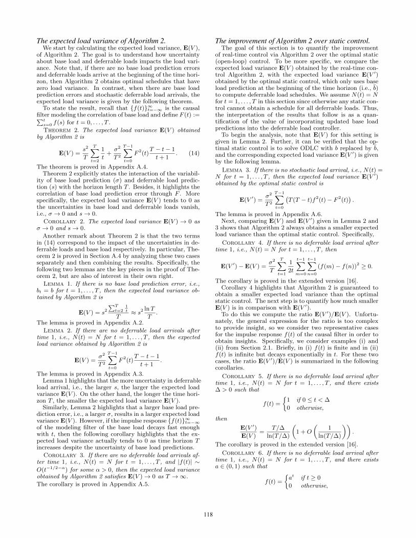
load and renewable generation. The non-deferrable loadtraces used in the experiments come from the average resi-dential load in the service area of Southern California Edi-son in 2012 [28]. In the simulations, we assume that non-deferrable load is precisely known so that uncertainties inthe base load only come from renewable generation. In par-ticular, non-deferrable load over the time horizon of a dayis taken to be the average over the 366 days in 2012 as inFigure 2(a), and assumed to be known to the utility at thebeginning of the time horizon. In practice, non-deferrableload at the substation feeder level can be predicted within1–3% root-mean-square error looking 24 hours ahead [13].
The renewable generation traces we use come from the10-minute historical data for total wind power generation ofthe Alberta Electric System Operator from 2004 to 2009 [3].In the simulations, we scale the wind power generation sothat its average over the 6 years corresponds to a numberof penetration levels in the range between 5% and 30%, andpick the wind power generation of a randomly chosen day asthe renewable generation during each run. Figure 2(b) showsthe wind power generation for four representative days, onefor each season, after scaling to 20% penetration.
We assume that the renewable generation is not preciselyknown until it is realized, but that a prediction of the gen-eration, which improves over time, is available to the utility.The modeling of prediction evolution over time is according
to a martingale forecasting process [18,19], which is a stan-dard model for an unbiased prediction process that improvesover time.
Specifically, the prediction model is as follows: For windgeneration w(τ) at time τ , the prediction error wt(τ)−w(τ)at time t < τ is the sum of a sequence of independent randomvariables ns(τ) as
wt(τ) = w(τ) +
τ∑s=t+1
ns(τ), 0 ≤ t < τ ≤ T.
Here w0(τ) is the wind prediction without any observation,i.e., the expected wind generation w̄(τ) at the beginning ofthe time horizon (used by static control).
The random variables ns(τ) are assumed to be Gaussianwith mean 0. Their variances are chosen as
E(n2s(τ)) =
σ2
τ − s+ 1, 1 ≤ s ≤ τ ≤ T
where σ > 0 is such that the root-mean-square prediction er-ror√
E(w0(T )− w(T ))2 looking T time slots (i.e., 24 hours)ahead is 0%–22.5% of the nameplate wind generation ca-pacity.2 According to this choice of the variances of ns(τ),root-mean-square prediction error only depends on how farahead the prediction is, in particular as in Figure 2(c). Thischoice is motivated by [17].
Deferrable loads.For simplicity, we consider the hypothetical case where all
deferrable loads are electric vehicles. Since historical datafor electric vehicle usage is not available, we are forced touse synthetic traces for this component of the experiments.Specifically, in the simulations the electric vehicles are con-sidered to be identical, each requests 10kWh electricity bya deadline 8 hours after it arrives, and each must consumepower at a rate within [0, 3.3]kW after it arrives and beforeits deadline.
In the simulations, the arrival process starts at 20:00 andends at 12:00 the next day so that the deadlines of all electricvehicles lie within the time horizon of 24 hours. In each timeslot during the arrival process, we assume that the num-ber of arriving electric vehicles is uniformly distributed in[0.8λ, 1.2λ], where λ is chosen so that electric vehicles (onaverage) account for 5%–30% of the non-deferrable loads.While this synthetic workload is simplistic, the results wereport are representative of more complex setups as well.
Uncertainty about deferrable load arrivals is captured asfollows. The prediction E(A(t)) of future deferrable loadtotal energy request is simply the arrival rate λ times thelength of the rest of the arrival process T ′ − t where T ′ isthe end of the arrival process (12:00), i.e.,
E(A(t)) = λ(T ′ − t), t = 1, . . . , T ′.
If t > T ′, i.e., the deferrable load arrival process has ended,then E(A(t)) = 0.
Baselines for comparison.Our goal in the simulations is to contrast the performance
of Algorithm 2 with a number of common benchmarks totease apart the impact of real-time control and the impactof different forms of uncertainty. To this end, we considerfour controllers in our experiments:
2Average wind generation is 15% of the nameplate capacity,so the root-mean-square prediction error looking T time slotsahead is 0%–150% the average wind generation.
119
20:00 4:00 12:00 20:000.4
0.5
0.6
0.7
0.8
0.9
1
1.1
time of day
non−
defe
rrable
load (
kW
/household
)
(a) non-deferrable load
20:00 4:00 12:00 20:000
0.1
0.2
0.3
0.4
time of day
renew
able
genera
tion (
kW
/household
)
Jan. 1st~2nd, 2006Apr. 1st~2nd, 2007Jul. 1st~2nd, 2008Oct. 1st~2nd, 2009
(b) wind generation
0h 8h 16h 24h0
20
40
60
80
100
time looking ahead
norm
aliz
ed w
ind p
redic
tion e
rror
(%)
(c) prediction error over time
Figure 2: Illustration of the traces used in the experiments. (a) shows the average residential load in theservice area of Southern California Edison in 2012. (b) shows the total wind power generation of the AlbertaElectric System Operator scaled to represent 20% penetration. (c) shows the normalized root-mean-squarewind prediction error as a function of the time looking ahead for the model used in the experiments.
(i) Offline optimal control: The controller has full knowl-edge about the base load and deferrable loads, andsolves the ODLC problem offline. It is not realistic inpractice, but serves as a benchmark for the other con-trollers since offline optimal control obtains the small-est possible load variance.
(ii) Static control with exact deferrable load arrival infor-mation: The controller has full knowledge about de-ferrable loads (including those that have not arrived),but uses only the prediction of base load that is avail-able at the beginning of the time horizon to compute adeferrable load schedule that minimizes the expectedload variance. This static control is still unrealisticsince a deferrable load is known only after it arrives.But, this controller corresponds to what is consideredin prior works, e.g., [14,15,25].
(iii) Real-time control with exact deferrable load arrival in-formation. The controller has full knowledge about de-ferrable loads (including those that have not arrived),and uses the prediction of base load that is availableat the current time slot to update the deferrable loadschedule by minimizing the expected load variance togo, i.e., Algorithm 2 with N(t) = N for t = 1, . . . , T .The control is unrealistic since a deferrable load isknown only after it arrives; however it provides thenatural comparison for case (ii) above.
(iv) Real-time control without exact deferrable load arrivalinformation, i.e., Algorithm 2. This corresponds tothe realistic scenario where only predictions are avail-able about future deferrable loads and base load. Thecomparison with case (iii) highlights the impact of de-ferrable load arrival uncertainties.
The performance measure that we show in all plots is the“suboptimality” of the controllers, which we define as
η :=V − V opt
V opt,
where V is the load variance obtained by the controller andV opt is the load variance obtained by the offline optimal, i.e.,case (i) above. Thus, the lines in the figures correspond tocases (ii)-(iv).
5.2 Experimental resultsOur experimental results focus on two main goals: (i) un-
derstanding the impact of prediction accuracy on the ex-pected load variance obtained by deferrable load control
algorithms, and (ii) contrasting the real-time (closed-loop)control of Algorithm 2 with the optimal static (open-loop)controller. We focus on the impact of three key factors: windprediction error, the penetration of deferrable load, and thepenetration of renewable energy.
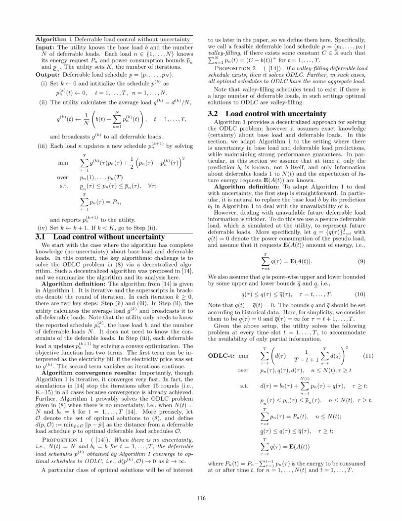
The impact of prediction error.To study the impact of prediction error, we fix the pene-
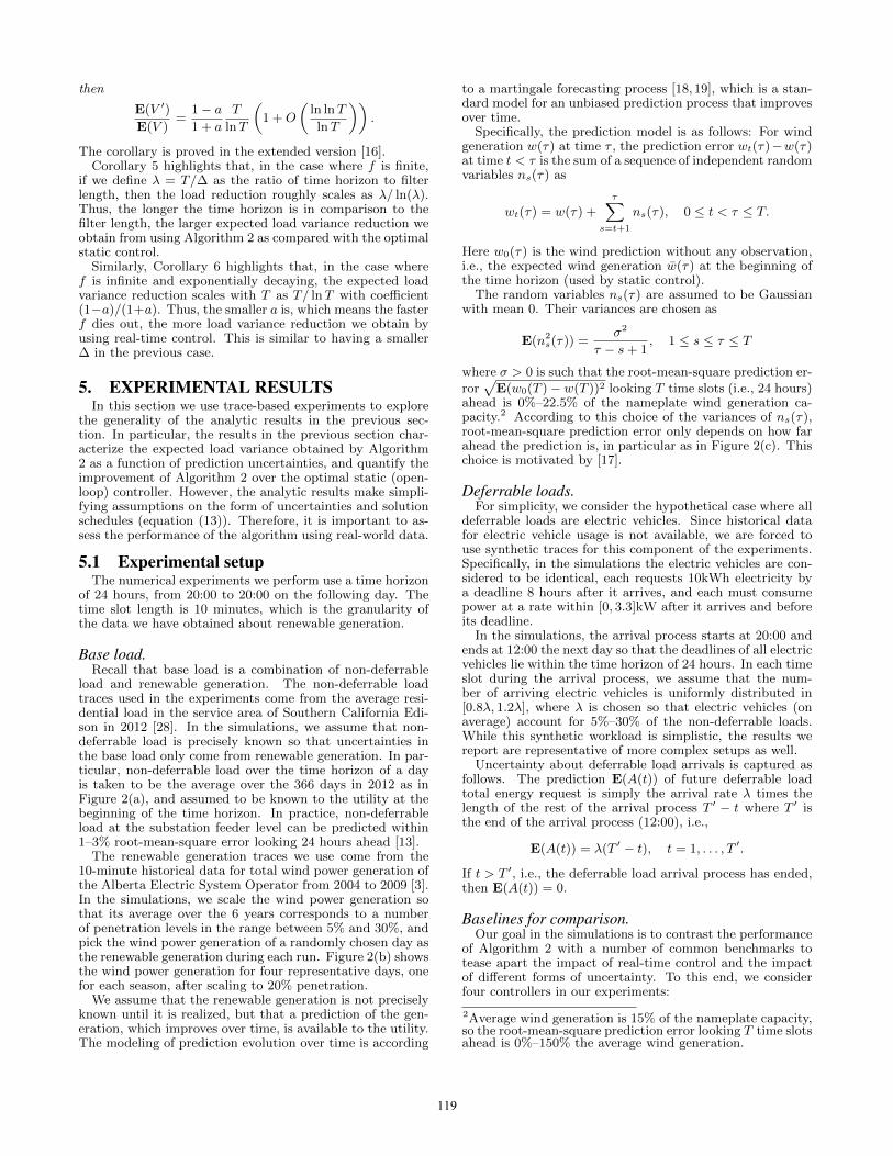
tration of both renewable generation (wind) and deferrableloads at 10% of non-deferrable load, and simulate the loadvariance obtained under different levels of root-mean-squarewind prediction errors (0%–22.5% of the nameplate capac-ity looking 24 hours ahead). The results are summarized inFigure 3(a). It is not surprising that suboptimality of boththe static and the real-time controllers that have exact infor-mation about deferrable load arrivals is zero when the windprediction error is 0, since there is no uncertainty for thesecontrollers in this case.
0 5 10 15 200
5
10
15
wind prediction error (%)
suboptim
alit
y (
%)
static w/ arrival info.real−time w/o arrival info.real−time w/ arrival info.
(a) Wind and deferrable loadpenetration are both 10%.
0 5 10 15 200
20
40
60
80
wind prediction error (%)
suboptim
alit
y (
%)
static w/ arrival info.real−time w/o arrival info.real−time w/ arrival info.
(b) Wind and deferrable loadpenetration are both 20%.
Figure 3: Illustration of the impact of wind predic-tion error on suboptimality of load variance.
As prediction error increases, the suboptimality of boththe static and the real-time control increases. However, no-tably, the suboptimality of real-time control grows muchmore slowly than that of static control, and remains small(<4.7%) if deferrable load arrivals are known, over the wholerange 0%–22.5% of wind prediction error. At 22.5% predic-tion error, the suboptimality of static control is 4.2 timesthat of real-time control. This highlights that real-time con-trol mitigates the influence of imprecise base load predictionover time.
Moving to the scenario where deferrable load arrivals arenot known precisely, we see that the impact of this inexactinformation is less than 6.6% of the optimal variance. How-
120
ever, real-time control yields a load variance that is surpris-ingly resilient to the growth of wind prediction error, andeventually beats the optimal static control at around 10%wind prediction error, even though the optimal static con-trol has exact knowledge of deferrable loads and the adaptivecontrol does not.
As prediction error increases, the suboptimality of thereal-time control with or without deferrable load arrival in-formation gets close, i.e., the benefit of knowing additionalinformation on future deferrable load arrivals vanishes asbase load uncertainty increases. This is because the addi-tional information is used to overfit the base load predictionerror.
The same comparison is shown in Figure 3(b) for the casewhere renewable and deferrable load penetration are both20%. Qualitatively the conclusions are the same, however atthis higher penetration the contrast between the resilienceof adaptive control and static control is magnified, whilethe benefit of knowing deferrable load arrival informationis minified. In particular, real-time control without arrivalinformation beats static control with arrival information, ata lower (around 7%) wind prediction error, and knowingdeferrable load arrival information does not reduce subopti-mality of real-time control with 22.5% wind prediction error.
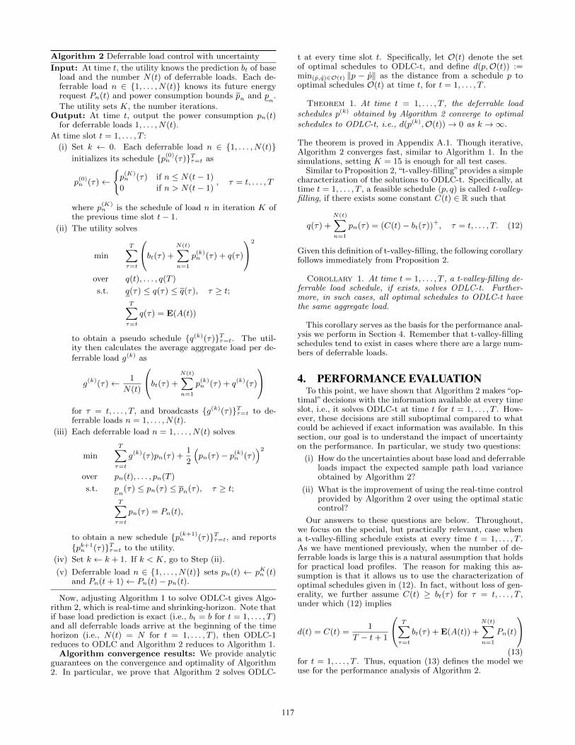
The impact of deferrable load penetration.Next, we look at the impact of deferrable load penetration
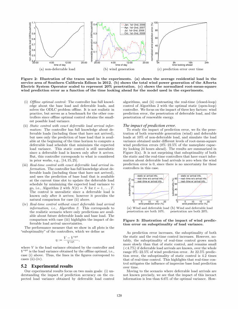
on the performance of the various controllers. To do this, wefix the wind penetration level to be 20% and wind predic-tion error looking 24 hours ahead to be 18%, and simulatethe load variance obtained under different deferrable loadpenetration levels (5%–30%). The results are summarizedin Figure 4(a).
5 10 15 20 25 300
50
100
150
deferrable load penetration (%)
suboptim
alit
y (
%)
static w/ arrival info.real−time w/o arrival info.real−time w/ arrival info.
(a) Impact of deferrable loadpenetration
5 10 15 20 250
20
40
60
80
wind penetration (%)
suboptim
alit
y (
%)
static w/ arrival info.real−time w/o arrival info.real−time w/ arrival info.
(b) Impact of wind penetra-tion
Figure 4: Suboptimality of load variance as a func-tion of (a) deferrable load penetration and (b) windpenetration. In (a) the wind penetration is 20%and in (b) the deferrable load penetration is 20%.In both, the wind prediction error looking 24 hoursahead is 18%.
Not surprisingly, if future deferrable loads are known anduncertainty only comes from base load prediction error, thenthe suboptimality of real-time control is very small (<11.2%)over the whole range 5%–30% of deferrable load penetration,while the suboptimality of static control increases with de-ferrable load penetration, up to as high as 166% (14.9 timesthat of real-time control) at 30% deferrable load penetration.
However, without knowing future deferrable loads, thesuboptimality of real-time control increases with the de-ferrable load penetration. This is because larger amount ofdeferrable loads introduces larger uncertainties in deferrableload arrivals. But the suboptimality remains smaller thanthat of static control over the whole range 5%–30% of de-ferrable load penetration. The highest suboptimality 25.7%
occurs at 30% deferrable load penetration, and is less than1/6 of the suboptimality of static control, which assumesexact deferrable load arrival information.
The impact of renewable penetration.Finally, we study the impact of renewable penetration.
To do this we fix the deferrable load penetration level to be20% and the wind prediction error looking 24 hours aheadto be 18%, and simulate the load variance obtained by the 4test cases under different wind penetration levels (5%–25%).The results are summarized in Figure 4(b).
A key observation is that if future deferrable loads areknown and uncertainty only comes from base load predic-tion error, then the suboptimality of real-time control growsmuch slower than that of static control, as wind penetrationlevel increases. As explained before, this highlights that real-time control mitigates the impact of base load predictionerror over time. In fact, the suboptimality of real-time con-trol is small (<15%) over the whole range 5%–25% of windpenetration levels. Of course, without knowledge of futuredeferrable loads, the suboptimality of real-time control be-comes bigger. However, it still eventually outperforms theoptimal static controller at around 6% wind penetration, de-spite the fact that the optimal static controller is using exactinformation about deferrable loads.
6. CONCLUDING REMARKSWe have proposed a real-time algorithm for decentralized
deferrable load control that can schedule a large number ofdeferrable loads to compensate for the random fluctuationsin renewable generation. At any time, the algorithm in-corporates updated predictions about deferrable loads andrenewable generation to minimize the expected load vari-ance to go. Further, we have derived an explicit expressionfor the expected aggregate load variance obtained by the al-gorithm by modeling the base load prediction updates as aWiener filtering process. Additionally, we have highlightedthe importance of the expression by using it to evaluate theimprovement of real-time control over static control. Inter-estingly, the sub-optimality of static control is O(T/ lnT )times that of real-time control in two representative cases ofbase load prediction updates. The qualitative insights fromthe analytic results were validated using trace-based simu-lations, which confirm that the algorithm has significantlysmaller sub-optimality than the optimal static control.
There remain many open questions on deferrable load con-trol. For example, is it possible to reduce the communicationand computation requirements of the proposed algorithm byassuming achievability of t-valley-filling? How to extend thealgorithm to a receding horizon implementation? Addition-ally, how to apply the technique used here to incorporateprediction evolution for other demand response settings.
7. ACKNOWLEDGEMENTThis work was supported by NSF NetSE grant CNS 0911041,
ARPA-E grant DE-AR0000226, Southern California Edison,National Science Council of Taiwan, R.O.C, grant NSC 101-3113-P-008-001, Resnick Institute, Okawa Foundation, NSFCNS 1312390, NSF grant CNS 0846025, and DoE grant DE-EE000289.
8. REFERENCES[1] S. Acha, T. C. Green, and N. Shah. Effects of optimised
plug-in hybrid vehicle charging strategies on electricdistribution network losses. In IEEE PES Transmission andDistribution Conference and Exposition, pages 1–6, 2010.
121
[2] D. J. Aigner and J. G. Hirschberg. Commercial/industrialcustomer response to time-of-use electricity prices: Someexperimental results. The RAND Journal of Economics,16(3):341–355, 1985.
[3] Alberta Electric System Operator. Wind power / ail data,2009. http://www.aeso.ca/gridoperations/20544.html.
[4] J.-Y. L. Boudec and D.-C. Tomozei. Satisfiability of elasticdemand in the smart grid. arXiv preprint arXiv:1011.5606,2010.
[5] California Public Utilities Commission. Zero net energyaction plan, 2008. http://www.cpuc.ca.gov/NR/rdonlyres/6C2310FE-AFE0-48E4-AF03-530A99D28FCE/0/ZNEActionPlanFINAL83110.pdf.
[6] M. Caramanis and J. Foster. Management of electric vehiclecharging to mitigate renewable generation intermittencyand distribution network congestion. In IEEE CDC, pages4717–4722, 2009.
[7] L. Chen, N. Li, S. H. Low, and J. C. Doyle. Two marketmodels for demand response in power networks. In IEEESmartGridComm, pages 397–402, 2010.
[8] S. Chen and L. Tong. iems for large scale charging ofelectric vehicles: architecture and optimal online scheduling.In IEEE SmartGridComm, pages 629–634, 2012.
[9] A. Conejo, J. Morales, and L. Baringo. Real-time demandresponse model. IEEE Transactions on Smart Grid,1(3):236–242, 2010.
[10] S. Deilami, A. Masoum, P. Moses, and M. Masoum.Real-time coordination of plug-in electric vehicle chargingin smart grids to minimize power losses and improvevoltage profile. IEEE Transactions on Smart Grid,2(3):456–467, 2011.
[11] Department of Energy. The smart grid: an introduction,2008. http://energy.gov/sites/prod/files/oeprod/DocumentsandMedia/DOE_SG_Book_Single_Pages%281%29.pdf.
[12] Department of Energy. One million electric vehicles by2015, 2011.http://www1.eere.energy.gov/vehiclesandfuels/pdfs/1_million_electric_vehicles_rpt.pdf.
[13] E. A. Feinberg and D. Genethliou. Load forecasting. InApplied Mathematics for Restructured Electric PowerSystems, Power Electronics and Power Systems, pages269–285. Springer US, 2005.
[14] L. Gan, U. Topcu, and S. H. Low. Optimal decentralizedprotocol for electric vehicle charging. In IEEE CDC, pages5798–5804, 2011.
[15] L. Gan, U. Topcu, and S. H. Low. Stochastic distributedprotocol for electric vehicle charging with discrete chargingrate. In IEEE PES General Meeting, pages 1–8, 2012.
[16] L. Gan, A. Wierman, U. Topcu, N. Chen, and S. H. Low.Real-time deferrable load control: handling theuncertainties of renewable generation, 2013. Technicalreport, available athttp://www.its.caltech.edu/~lgan/index.html.
[17] G. Giebel, R. Brownsword, G. Kariniotakis, M. Denhard,and C. Draxl. The State-Of-The-Art in Short-TermPrediction of Wind Power. ANEMOS.plus, 2011.
[18] S. C. Graves, D. B. Kletter, and W. B. Hetzel. A dynamicmodel for requirements planning with application to supplychain optimization. Manufacturing & Service OperationManagement, 1(1):50–61, 1998.
[19] S. C. Graves, H. C. Meal, S. Dasu, and Y. Qiu. Two-stageproduction planning in a dynamic environment, 1986.http://web.mit.edu/sgraves/www/papers/GravesMealDasuQiu.pdf.
[20] N. Hatziargyriou, H. Asano, R. Iravani, and C. Marnay.Microgrids. IEEE Power and Energy Magazine, 5(4):78–94,2007.
[21] Y.-Y. Hsu and C.-C. Su. Dispatch of direct load controlusing dynamic programming. IEEE Transactions on PowerSystems, 6(3):1056–1061, 1991.
[22] M. Ilic, J. Black, and J. Watz. Potential benefits ofimplementing load control. In IEEE PES Winter Meeting,volume 1, pages 177–182, 2002.
[23] N. Li, L. Chen, and S. H. Low. Optimal demand response
based on utility maximization in power networks. In IEEEPES General Meeting, pages 1–8, 2011.
[24] Q. Li, T. Cui, R. Negi, F. Franchetti, and M. D. Ilic.On-line decentralized charging of plug-in electric vehicles inpower systems. arXiv:1106.5063, 2011.
[25] Z. Ma, D. Callaway, and I. Hiskens. Decentralized chargingcontrol for large populations of plug-in electric vehicles. InIEEE CDC, pages 206–212, 2010.
[26] K. Mets, T. Verschueren, W. Haerick, C. Develder, andF. De Turck. Optimizing smart energy control strategies forplug-in hybrid electric vehicle charging. In IEEE/IFIPNOMS Wksps, pages 293–299, 2010.
[27] National Institute of Standards and Technology. Nistframework and roadmap for smart grid interoperabilitystandards, 2010.http://www.nist.gov/public_affairs/releases/upload/smartgrid_interoperability_final.pdf.
[28] Southern California Edison. 2012 static load profiles, 2012.http://www.sce.com/005_regul_info/eca/DOMSM12.DLP.
[29] A. Subramanian, M. Garcia, A. Dominguez-Garcia,D. Callaway, K. Poolla, and P. Varaiya. Real-timescheduling of deferrable electric loads. In ACC, pages3643–3650, 2012.
[30] Wikipedia. Krasovskii-lasalle principle. http://en.wikipedia.org/wiki/Krasovskii-LaSalle_principle.
[31] Wikipedia. Wiener filter.http://en.wikipedia.org/wiki/Wiener_filter.
APPENDIXA. PROOFS
In this section, we only include proofs of the main resultsdue to space restrictions. The remainder of the proofs canbe found in the extended version [16].
A.1 Proof of Theorem 1For brevity and without loss of generality, we prove The-
orem 1 for t = 1 only. Thus, we can abbreviate bt and N(t)by b and N respectively without introducing confusion.
For feasible p, q to ODLC-t and p = (p1, . . . , pN ), define
L(p, q) =
T∑τ=1
(b(τ) +
N∑n=1
pn(τ) + q(τ)
)2
.
Since the sum of the aggregate load∑Tτ=1 d(τ) is a constant,
minimizing the `2 norm of the aggregate load is equivalentto minimizing its variance. Hence, if subject to the sameconstraints, the minimizer of L is also the solution to ODLC-t. According to the proof of Proposition 1 in [14], we have
L(p(k+1), q(k)) ≤ L(p(k), q(k))
for k ≥ 0, and the equality is attained if and only if p(k+1) =p(k) and p(k) minimizes L(p, q(k)) over all feasible p, i.e., (thefirst order optimality condition)⟨
b+
N∑n=1
p(k)n + q(k), p′n − p(k)n
⟩≥ 0
for n = 1, . . . , N and all feasible p′n. According to Step (ii)of Algorithm 2, it is straightforward that
L(p(k+1), q(k+1)) ≤ L(p(k+1), q(k))
for k ≥ 0, and the equality is attained if and only if q(k+1) =q(k) and q(k) minimizes L(p(k+1), q) over all feasible q, i.e.,(the first order optimality condition)⟨
b+
N∑n=1
p(k+1)n + q(k), q′ − q(k)
⟩≥ 0
122
for all feasible q′. It then follows that
L(p(k+1), q(k+1)) ≤ L(p(k), q(k))
and the equality if attained if and only if (p(k+1), q(k+1)) =
(p(k), q(k)), and⟨b+
N∑n=1
p(k)n + q(k), p′n − p(k)n
⟩≥ 0,⟨
b+
N∑n=1
p(k)n + q(k), q′ − q(k)⟩≥ 0
for all feasible p and q, i.e., (p(k), q(k)) minimizes L(p, q).
Then by Lasalle’s Theorem [30], we have d(p(k),O(t)) → 0as k →∞. �
A.2 Proof of Lemma 1When bt = b and E(a(t)) = λ for t = 1, . . . , T , the model
(13) for Algorithm 2 reduces to
d(t) =1
T − t+ 1
T∑τ=t
b(τ) + λ(T − t) +
N(t)∑n=1
Pn(t)
(15)
for t = 1, . . . , T . Then
(T − t+ 1)d(t) =
T∑τ=t
b(τ) + λ(T − t) +
N(t)∑n=1
Pn(t)
(T−t+2)d(t−1) =
T∑τ=t−1
b(τ)+λ(T−t+1)+
N(t−1)∑n=1
Pn(t−1)
for t = 2, . . . , T . Subtract the two equations and simplify
using the fact that b(t− 1) +∑N(t−1)n=1 (Pn(t− 1)− Pn(t)) =
b(t− 1) +∑N(t−1)n=1 pn(t− 1) = d(t− 1) and the definition of
a(t) to obtain
d(t)− d(t− 1) =1
T − t+ 1(a(t)− λ)
for t = 2, . . . , T . Substituting t = 1 into (15), it can be
verified that d(1) = λ+∑Tτ=1 b(τ)/T+(a(1)−λ)/T , therefore
d(t) = λ+1
T
T∑τ=1
b(τ) +
t∑τ=1
1
T − τ + 1(a(τ)− λ)
for t = 1, . . . , T . The average aggregate load is
u =1
T
T∑t=1
d(t) = λ+1
T
(T∑τ=1
b(τ) +
T∑τ=1
(a(τ)− λ)
).
Hence,
E(d(t)− u)2
= E
(t∑
τ=1
1
T − τ + 1(a(τ)− λ)− 1
T
T∑τ=1
(a(τ)− λ)
)2
= E
(t∑
τ=1
τ − 1
T (T − τ + 1)(a(τ)− λ)− 1
T
T∑τ=t+1
(a(τ)− λ)
)2
=s2
T 2
(t∑
τ=1
(τ − 1)2
(T − τ + 1)2+ T − t
)
for t = 1, . . . , T . The last equality holds because (a(τ)− λ)are independent for all τ and each of them have mean zeroand variance s2. It follows that
E(V ) =1
T
T∑t=1
E(d(t)− u)2
=s2
T 3
(T∑t=1
t∑τ=1
(τ − 1)2
(T − τ + 1)2+
T∑t=1
(T − t)
)
=s2
T 3
(T∑τ=1
(τ − 1)2
T − τ + 1+
T∑t=1
(T − t)
)
=s2
T 3
(T∑t=1
(T − t)2
t+
T∑t=1
(T − t)tt
)
= s2∑Tt=2
1t
T∼ s2 lnT
T. �
A.3 Proof of Lemma 2In the case where no deferrable arrival after t = 1, i.e.,
N(t) = N for t = 1, . . . , T , the model (13) for Algorithm 2reduces to
(T − t+ 1)d(t) =
T∑τ=t
bt(τ) +
N∑n=1
Pn(t) (16)
for t = 1, . . . , T . Substitute t by t− 1 to obtain
(T − t+ 2)d(t− 1) =
T∑τ=t−1
bt−1(τ) +
N∑n=1
Pn(t− 1)
for t = 2, . . . , T . Subtract the two equations to obtain
(T − t+ 1)d(t)− (T − t+ 2)d(t− 1)
=
T∑τ=t
e(t)f(τ − t)− b(t− 1)−N∑n=1
pn(t− 1)
= e(t)F (T − t)− d(t− 1),
which implies
d(t)− d(t− 1) =1
T − t+ 1e(t)F (T − t)
for t = 2, . . . , T . Substituting t = 1 into (16) and recallingthe definition of bt in (1), it can be verified that
d(1) =1
T
(N∑n=1
Pn +
T∑τ=1
b̄(τ)
)+
1
Te(1)F (T − 1).
Therefore,
d(t) =1
T
(N∑n=1
Pn +
T∑τ=1
b̄(τ)
)+
t∑τ=1
1
T − τ + 1e(τ)F (T − τ)
for t = 1, . . . , T . The average aggregate load is
u =1
T
(N∑n=1
Pn +
T∑t=1
b̄(t)
)+
1
T
T∑τ=1
e(τ)F (T − τ).
123
Hence,
E(d(t)− u)2
= E
(t∑
τ=1
1
T − τ + 1e(τ)F (T − τ)−
T∑τ=1
1
Te(τ)F (T − τ)
)2
= E
(t∑
τ=1
τ − 1
T (T − τ + 1)e(τ)F (T − τ)
−T∑
τ=t+1
1
Te(τ)F (T − τ)
)2
=σ2
T 2
(t∑
τ=1
(τ − 1)2
(T − τ + 1)2F 2(T − τ) +
T∑τ=t+1
F 2(T − τ)
)
for t = 1, . . . , T . The last equality holds because e(τ) areuncorrelated random variables with mean zero and varianceσ2. It follows that
E(V ) =1
T
T∑t=1
E(d(t)− u)2
=σ2
T 3
T∑t=1
(t∑
τ=1
(τ − 1)2
(T − τ + 1)2F 2(T − τ) +
T∑τ=t+1
F 2(T − τ)
)
=σ2
T 3
T∑τ=1
F 2(T − τ)(τ − 1)2
T − τ + 1+σ2
T 3
T∑τ=2
(τ − 1)F 2(T − τ)
=σ2
T 2
T∑τ=1
F 2(T − τ)τ − 1
T − τ + 1=σ2
T 2
T−1∑t=0
F 2(t)T − t− 1
t+ 1.�
A.4 Proof of Theorem 2Similar to the proof of Lemma 1 and 2, use the model (13)
to obtain
d(t) = λ+1
T
T∑τ=1
b̄(τ) +
t∑τ=1
1
T − τ + 1(e(τ)F (T − τ) + a(τ)− λ)
for t = 1, . . . , T and
u = λ+1
T
T∑τ=1
b̄(τ) +
T∑τ=1
1
T(e(τ)F (T − τ) + a(τ)− λ) .
Hence,
E(d(t)− u)2
= E
(t∑
τ=1
1
T − τ + 1e(τ)F (T − τ)−
T∑τ=1
1
Te(τ)F (T − τ)
)2
+E
(t∑
τ=1
1
T − τ + 1(a(τ)− λ)−
T∑τ=1
1
T(a(τ)− λ)
)2
.
The first term is exactly that in Lemma 2, and the secondterm is exactly that in Lemma 1. Hence, the expected loadvariance is
E(V ) =σ2
T 2
T−1∑t=0
F 2(t)T − t− 1
t+ 1+s2
T
T∑t=2
1
t. �
A.5 Proof of Corollary 3If |f(t)| ∼ O(t−1/2−α) for some α > 0, then |f(t)| ≤
Ct−1/2−α for some C > 0 and all t ≥ 1. Without loss of
generality, assume that 0 < α < 1/2 and C ≥ (1− 2α)/(1 +2α). Then F (0) = 1 and
|F (t)| =
∣∣∣∣∣t∑
τ=0
f(τ)
∣∣∣∣∣ ≤ 1 +
t∑τ=1
Cτ−1/2−α ≤ 2C
1− 2αt1/2−α
for t = 1, . . . , T . The last inequality holds because C ≥(1− 2α)/(1 + 2α). Therefore it follows from Lemma 2 that
E(V ) ≤ σ2
T
T−1∑s=0
F 2(s)1
s+ 1
≤ σ2
T+σ2
T
T−1∑s=1
4C2
(1− 2α)2s1−2α 1
s+ 1
≤ σ2
T+σ2
T
4C2
(1− 2α)2
T−1∑s=1
1
s2α
≤ σ2
T+
4σ2C2
(1− 2α)2T+
4σ2C2
(1− 2α)3T 2α.
Hence, E(V )→ 0 as T →∞. �
A.6 Proof of Lemma 3The aggregate load d obtained by the optimal static algo-
rithm is
d(t) =1
T
(N∑n=1
Pn +
T∑τ=1
b̄(τ)
)− b̄(t) + b(t)
=1
T
(N∑n=1
Pn +
T∑τ=1
b̄(τ)
)+
T∑τ=1
e(τ)f(t− τ)
for t = 1, . . . , T . Hence,
E(d(t)− u)2
= E
(T∑τ=1
e(τ)
(f(t− τ)− 1
TF (T − τ)
))2
=σ2
T 2
T∑τ=1
T 2f2(t− τ)− 2Tf(t− τ)F (T − τ) + F 2(T − τ)
for t = 1, . . . , T . It follows that
E(V ′) =1
T
T∑t=1
E(d(t)− u)2
=σ2
T
T∑t=1
T∑τ=1
f2(t− τ)− 2σ2
T 2
T∑τ=1
F (T − τ)
T∑t=1
f(t− τ)
+σ2
T 2
T∑τ=1
F 2(T − τ)
=σ2
T
T∑t=1
t−1∑τ=0
f2(τ)− σ2
T 2
T∑τ=1
F 2(T − τ)
=σ2
T
T−1∑τ=0
(T − τ)f2(τ)− σ2
T 2
T−1∑τ=0
F 2(τ)
=σ2
T 2
T−1∑t=0
(T (T − t)f2(t)− F 2(t)
). �
124