Design and Construction of a Fourier Transform Soft X-ray Interferometer

A thesis submitted to the faculty of San Francisco State University

in partial fulfillment of the requirements for the degree

Master of Science in

Physics

by

John Spring

San Francisco, California

May, 2000

CERTIFICATION OF APPROVAL

I certify that I have read Design and Construction of a Fourier Transform Soft X-

ray Interferometer by John Spring and that in my opinion this work meets the

criteria for approving a thesis submitted in partial fulfillment of the requirements

for the degree: Master of Science in Physics and San Francisco State

University.

__________________________________________ James Lockhart Professor of Physics __________________________________________ Adrienne Cool Professor of Physics __________________________________________ Malcolm Howells Staff Scientist, LBNL

DESIGN AND CONSTRUCTION OF A FOURIER TRANSFORM SOFT X-RAY INTERFEROMETER

John Spring San Francisco State University

May, 2000

Helium, with its two electrons and one nucleus, is a three-body system. One of the

models for investigating correlated electron motion in this system is auto-ionization,

produced via double excitation of the electrons. Predictions about the autoionization

spectrum of helium have differed from each other and from pre-liminary experimental

data. However, previous experiments have not been able to distinguish among the

theoretical predictions because their energy resolution is not high enough to resolve

the narrow linewidths of quasi-forbidden peaks and the resonances that appear in the

highest excited states. Consequently, a team of researchers at Lawrence Berkeley

National Laboratory have embarked on a project for building a high-resolution Fourier-

Transform Soft X-ray (or VUV) interferometer (FTSX) to provide definitive data to

answer remaining questions about the autoionization spectrum of helium. The design

and construction of this interferometer is described in detail below, including the use of

a flexure stage to provide the large path length difference necessary for high resolution

measurements, the manufacture of x-ray beamsplitters, a description of the software,

and the solution to the problems of stick-slip, vibration, and alignment. Current

progress of its development is also described, as well as future goals.

I certify that the Abstract is a correct representation of the content of this thesis. ___________________________________ ___________________ (Chair, Thesis Committee) (Date)

iv

ACKNOWLEDGEMENTS

There are several people I would like to thank for their help in completing this

work. Eddie Moler was my mentor in the physics and technical education

necessary for building the interferometer. Malcolm Howells and Zahid Hussain

directed the work with the wisdom borne of experience and great physical

insight. Scott Locklin has been an inspirational proponent of the possibilities

that our interferometer holds, and has continued the work with great energy. Jim

Lockhart, Adrienne Cool, Malcolm Howells, and Eddie Moler have taken the

time from their busy schedules to actually read this thesis and make very

constructive comments. (It couldn’t have been easy, folks.) Numerous people

contributed to the project, including Rob Duarte, Bob McGill, Ted Lauritzen, Troy

Barbie, Steve Irick, and all the people at the Advanced Light Source who put the

chamber and beamline together.

I would also like to thank my parents and friends for their unstinting and patient

support while I slogged my way through the work and thesis, and I would like to

especially thank Barbara Klatt for her patience, creativity, support, and ever-

outward vision, without which my world would have been dimmer.

v

TABLE OF CONTENTS

List of Figures.............................................................................................................vii

List of Appendices ....................................................................................................viii

Introduction................................................................................................................... 1

Overview of the Mach-Zehnder Interferometer......................................................... 5

Motivation for choosing the Mach-Zehnder configuration ....................................................5

Interferometry............................................................................................................... 9

Basic theory .................................................................................................................9

Determining Optical Component Tolerances ................................................................... 11

Description of Mach-Zehnder interferometer .........................................................22

Mechanical drive.......................................................................................................... 22

X-ray Optics................................................................................................................ 27

Data acquisition .......................................................................................................... 34

Measurement and rectification of tilt in stage movement......................................41

Explanation of problem and data................................................................................... 41

Rectification................................................................................................................ 48

Measurement and rectification of vibration and stick-slip.....................................50

Explanation of problem and data................................................................................... 50

Rectification................................................................................................................ 52

Alignment of the beamsplitters ................................................................................53

vi

Conclusions ...............................................................................................................56

Appendix 1: Derivation of Geometric Factor Used in Calculating Path Length Difference...................................................................................................................57

Appendix 2: Software Descriptions ........................................................................59

Dsp Program (dspacq.c) .............................................................................................. 59

VxWorks Program (VxServer.c).................................................................................... 75

vii

List of Figures

FIGURE 1: AUTOIONIZATION PROCESS FOR HELIUM................................................................................2 FIGURE 2: OPTICAL LAYOUT OF BEAMLINE 9.3.2 AT THE ALS...............................................................3 FIGURE 3: PHOTOGRAPH OF THE SOFT X-RAY INTERFEROMETER........................................................7 FIGURE 4: DIAGRAMS OF THE PATHS OF THE SPLIT BEAMS THROUGH THE X-RAY

INTERFEROMETER.....................................................................................................................................10 FIGURE 5: SIMPLIFIED RAY DIAGRAM FOR DESCRIBING SPHERICAL ERRORS................................14 FIGURE 6: RAY DIAGRAM FOR TILT ERRORS..............................................................................................17 FIGURE 7: SCHEMATIC DIAGRAM FOR DESCRIBING TILT ERRORS FOR ONE OF THE X-RAY

MIRRORS. .....................................................................................................................................................19 FIGURE 8: SCHEMATIC DIAGRAM FOR TILT ERRORS. THE MIRROR HAS BEEN ROTATED........20 FIGURE 9: FLEXURE TYPES.................................................................................................................................23 FIGURE 10: SCHEMATIC OF THE FLEXURE MECHANISM.........................................................................24 FIGURE 11: SCHEMATIC OF THE DRIVER......................................................................................................26 FIGURE 12: BEAMSPLITTER SCHEMATIC......................................................................................................28 FIGURE 13: TWO OF THE MANY ETCH PLANES...........................................................................................29 FIGURE 14: SCHEMATIC OF THE PRISM........................................................................................................30 FIGURE 15: THE SHACK INTERFEROMETER..................................................................................................32 FIGURE 16: TEST SETUP FOR DETERMINING PERPENDICULARITY OF A SIDE OF THE MIRROR

PRISM TO ITS BOTTOM ...........................................................................................................................33 FIGURE 17: SCHEMATIC OF FLEXURE MECHANISM, SHOWN DEFORMED. ......................................42 FIGURE 18: SCHEMATIC FOR TILT ANALYSIS. ...........................................................................................43 FIGURE 19: AUTOCOLLIMATOR SCHEMATIC..............................................................................................47 FIGURE 20: CORRECTION OF STAGE TILT WITH TAPER PIN ADJUSTMENT .....................................49 FIGURE 21: EXPANDED PLOT OF STAGE TILT AFTER CORRECTION. THE PITCH ERROR HAS

BEEN REDUCED TO 0.38 ΜRAD, RMS...................................................................................................50 FIGURE 22: THE STAGE IS MOVING IN A NEGATIVE DIRECTION AT -31.3 ΜM / SEC........................51 FIGURE 23: THESE ARE THE SAME DATA (OF FIGURE 22) AFTER THEY WERE FIT WITH A LINE52 FIGURE 24: POWER SPECTRUM OF MECHANICAL VIBRATIONS ...........................................................52 FIGURE 25: CONTACT POINTS ON A BEAMSPLITTER. .............................................................................54 FIGURE 26 ALIGNMENT SCAN USING INCOHERENT NEON LIGHT........................................................55 FIGURE A: PATH LENGTH CHANGE DUE TO MOVING ONE OF THE MIRRORS..................................58

viii

List of Appendices APPENDIX 1: DERIVATION OF GEOMETRIC FACTOR USED IN CALCULATING PATH LENGTH DIFFERENCE ................................................................................................... 57 APPENDIX 2: SOFTWARE DESCRIPTIONS...................................................................... 59

1

Introduction

Helium has two electrons and a nucleus, making it a three-body system. As such, it is

interesting for theoretical atomic physicists, who have made predictions about the

autoionization spectrum resulting from double excitation of the electrons1,2 .

Autoionization is a process in which both electrons are excited to energy levels above

the ground state; during the subsequent interaction of the continuum and the Rydberg-

like states of the two electrons' wavefunction, one of the electrons is ionized.

Specifically, the "inner" electron is excited into a shell N � 2, and the "outer" electron

into a shell n>N. More than thirty years ago, R.P. Madden and K. Codling discovered

that there is strong mixing among the doubly-excited states of helium.1 That is, while a

simple model of the two electrons behaving independently would suggest an absorption

spectrum including separate lines for the 2s and 2p series, they observed only one

series. In the paper following that one J.W. Cooper, U. Fano, and F. Prats suggested

some properties and a theory for correlated electron motion in doubly-excited helium.2

Need for higher resolution measurements

Theoretical predictions of the linewidths of the absorption spectrum of doubly-excited

helium have not agreed with each other nor adhered closely to previous

2

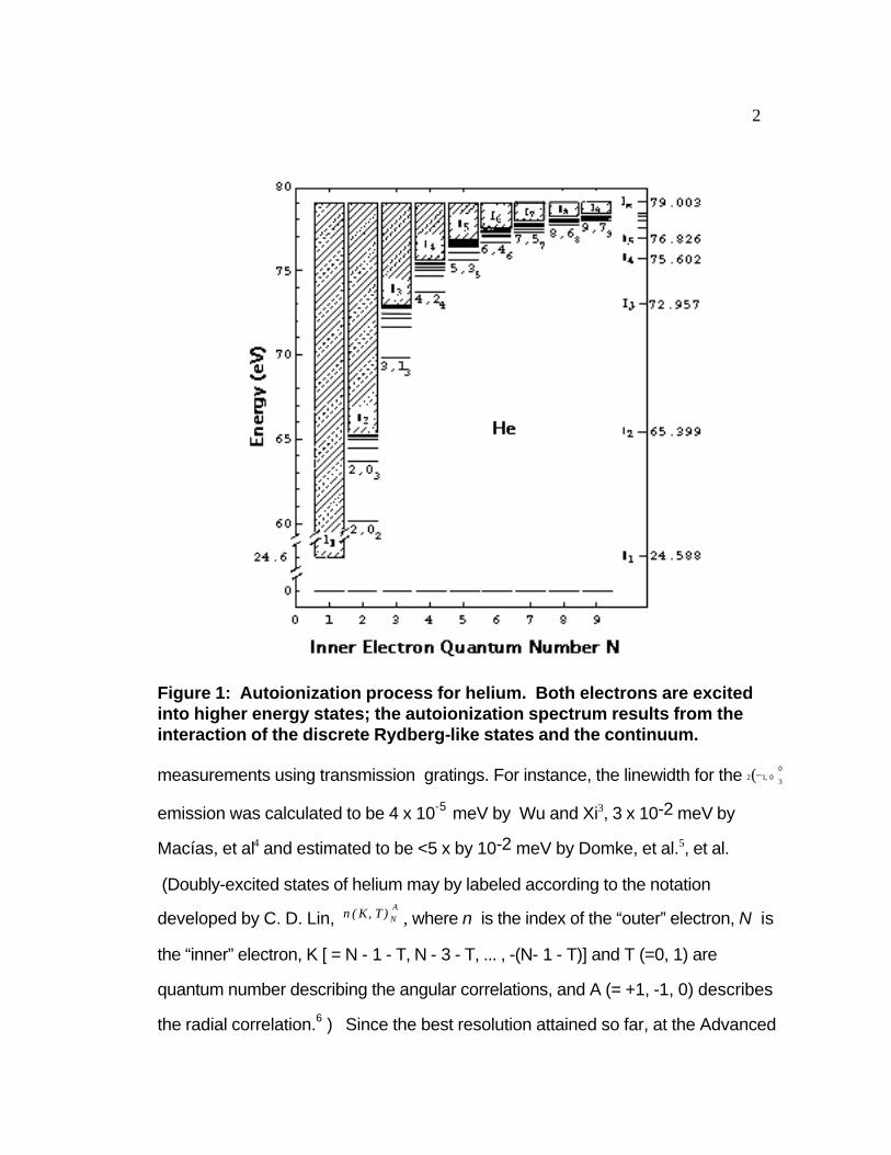
Figure 1: Autoionization process for helium. Both electrons are excited into higher energy states; the autoionization spectrum results from the interaction of the discrete Rydberg-like states and the continuum.

measurements using transmission gratings. For instance, the linewidth for the 2 −1, 0( )3

0

emission was calculated to be 4 x 10-5 meV by Wu and Xi3, 3 x 10-2 meV by

Macías, et al4 and estimated to be <5 x by 10-2 meV by Domke, et al.5, et al.

(Doubly-excited states of helium may by labeled according to the notation

developed by C. D. Lin, n ( K, T) NA

, where n is the index of the “outer” electron, N is

the “inner” electron, K [ = N - 1 - T, N - 3 - T, ... , -(N- 1 - T)] and T (=0, 1) are

quantum number describing the angular correlations, and A (= +1, -1, 0) describes

the radial correlation.6 ) Since the best resolution attained so far, at the Advanced

3

Light Source, was E/δE = 64,0007, it is clear that the higher resolution attainable

with this interferometer is required to answer these questions.

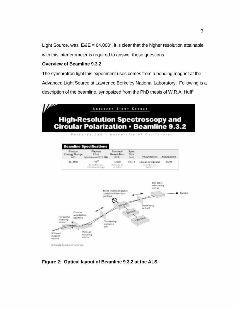
Overview of Beamline 9.3.2

The synchrotron light this experiment uses comes from a bending magnet at the

Advanced Light Source at Lawrence Berkeley National Laboratory. Following is a

description of the beamline, synopsized from the PhD thesis of W.R.A. Huff8

Figure 2: Optical layout of Beamline 9.3.2 at the ALS.

4

Light exits the synchrotron and strikes a cylindrical horizontal focusing mirror, whose

focus is at the exit slit. The light then goes through a circular polarization-selection

aperture (CPA). Bending magnet radiation is linearly polarized in the horizontal

plane of the centroid of the beam; above and below the horizontal plane, the vertical

component of polarization is nonzero, producing left and right circular polarization,

respectively. Thus, if the CPA is centered on the beam, horizontal linearly polarized

light is transmitted. Moving the CPA above the beam produces left elliptical

polarization that becomes more circular the farther the CPA is moved. Similar

motion below the beam produces right elliptical polarization.

Continuing downstream, the beam encounters the vertical focusing mirror, whose

focus is the entrance slit. Next, the beam encounters the entrance slit. The entrance

and exit slits determine the resolution of the beam according to the equation

∆λSW =WS 1d cos α

mr S 1

2

+W S 2 d cos β

mr S2

2

where WS1 = entrance slit width

WS2 = exit slit width

d = groove spacing if monochromator grating

α = incident angle of beam to grating

β = diffracted angle of beam from grating

m = diffraction order

rS1 = distance from entrance slit to grating

rS2 = distance from grating to exit slit

The beam next encounters the diffraction grating which, with the entrance and exit

slits, constitutes the monochromator. The energy of the transmitted beam is

5

selected from the energy band entering the monochromator by adjusting the angles

α and β and order m in the equation

±mλ = d(sin α + sin β)

where λ is the wavelength of the desired energy.

Overview of the Mach-Zehnder Interferometer

Motivation for choosing the Mach-Zehnder configuration

We chose a Mach-Zehnder configuration, and modified its original arrangement of

mirrors from a square to a rhombus. This was done to present grazing-incidence

angled surfaces to the x-ray beam, which would otherwise be absorbed by surfaces

at steeper angles. Two considerations led us to choose the Mach-Zehnder

interferometer over other suitable optical systems:

1. Grazing-incidence requirement. X-rays at high incidence angles are absorbed by

any material used in optics, so an optical system whose geometry exploits low

incidence angles has a higher throughput. For instance, the Michelson

interferometer has a single beamsplitter and two retroreflectors. The retroreflectors

require 90� incidence angles, so they would absorb most of the x-rays. Other

configurations of beamsplitters and mirrors suffer from similar limitations.

2. High energy resolution. This is the most important reason. Previous high-

resolution studies in this energy regime were carried out using reflection-grating

monochromators. (It is a spherical-grating monochromator that was used to get the

current highest resolution measurements of the autoionization spectrum of helium.)

For gratings resolution is determined by entrance and exit slit widths, the groove

spacing of the grating, the distance from the entrance slit to the grating, and the

distance from the grating to the exit slit. For interferometers, the energy resolution

6

is determined by the path-length difference between the two beams. (Actually, the

resolution is defined by the equation δE =hc∆x

where �x is the path-length difference

(PLD). Resolving power is a unitless measure of the quality of an optical system,

defined by R =EδE

.) The resolving power necessary to measure the narrow

linewidths of the quasi-forbidden peaks

(~10-5 eV) is on the order of 106 To get this resolving power for x-rays with an

energy of 65 eV requires a PLD of

∆x =hcδE

=hcR

E=

(1.24 eV − µm)(10 6 )65 eV

≅ 20 ,000 µm = 2.0 cm .

Introducing a 2 cm PLD while maintaining alignment of the separate beams (the

physical setup and optical tolerances will be described below) imposed

unprecedented technical requirements on the motion system . This range of travel

is several orders of magnitude beyond the range of piezoelectric ceramics, and a

motion system that uses a lead screw is simply too jerky and imprecise in its

motion. Flexure stages have proven themselves able to accomplish straight and

smooth motion for travel in the range 10-2 - 10-1 cm, so we used their design as a

model for our motion system.

7

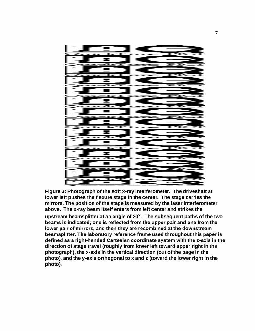
Figure 3: Photograph of the soft x-ray interferometer. The driveshaft at lower left pushes the flexure stage in the center. The stage carries the mirrors. The position of the stage is measured by the laser interferometer above. The x-ray beam itself enters from left center and strikes the upstream beamsplitter at an angle of 20o. The subsequent paths of the two beams is indicated; one is reflected from the upper pair and one from the lower pair of mirrors, and then they are recombined at the downstream beamsplitter. The laboratory reference frame used throughout this paper is defined as a right-handed Cartesian coordinate system with the z-axis in the direction of stage travel (roughly from lower left toward upper right in the photograph), the x-axis in the vertical direction (out of the page in the photo), and the y-axis orthogonal to x and z (toward the lower right in the photo).

8

Brief description of the Mach-Zehnder interferometer

The Mach-Zehnder interferometer comprises three subsystems: the x-ray optics, the

mechanical drive, and the data acquisition and control system (see figure 3). The x-

ray optics comprise the mirrors and beamsplitters. The purpose of the optics is to

split the x-ray beam into two beams, introduce a path length difference, and then

coherently recombine them. The four mirrors are supported by a flexure stage

(described below) and therefore move through its 1.5 cm range. The beamsplitters

are fixed to the frame of the flexure mechanism. In order for the separated beams to

recombine coherently, the optics must be aligned to within ~1 µrad. The reflecting

surfaces of the beamsplitters should be coplanar, and opposing sides of the

rhombus-shaped mirror assembly should be parallel. This alignment is done near

zero path length difference (ZPD) with the stage at rest. It became apparent that

manual alignment, by turning screws, was too crude, so we added computer-

controlled picomotors to automatically step through the small angles necessary for

proper alignment.

The mechanical drive comprises the flexure mechanism, a large hydraulic driver,

and an aluminum driveshaft connecting the two. Its purpose is to push and pull the x-

ray mirrors through a total distance of about 1.5 cm, with a minimum of vibration and

pitch angle. At the center of the flexure mechanism is a stage, a block of steel 2.62"

x 4.75" x 2.00", that supports the mirror assembly. The entire flexure mechanism

was cut from a single piece of steel using electric-discharge machining (EDM). The

hydraulic driver was designed to push against the rather large spring force of the

flexure mechanism, but at the same time could not introduce vibrations, into the

mirrors, whose frequencies were near those of the interference fringes as they

moved by the x-ray detector.

The data acquisition system comprises instrumentation and software for acquiring

three main channels of data: stage position, x-ray signal, and x-ray reference. The

control system controls the piston and beamsplitter alignment via picomotors.

9

Interferometry

Basic theory

An interferometer works by splitting a beam of light, sending the component beams

along two separate paths, and then coherently recombining them. Coherence

means that there is a constant phase between the recombining beams across a

cross-section of the reconstituted beam.

If we have a plane wave that has been split into two plane waves of equal amplitude

given by

E1 = E0(x)e-i(k"x - ωt)

E2 = E0(x)e-i(k"x - ωt + δ)

they will interfere with a phase difference δ, produced by an optical path difference.

The intensity of the sum of the two waves is given by

I = | E1 + E2 |2

= |E0(x)e-i(k"x - ωt)(1 + e-iδ)|2

= 2E02 (x)(1 + cos δ)

= 2E02(x)[1 + cos(2πσx)]

= B(σ)[1 + cos(2πσx)]

where x is the optical path difference, σ = 1/λ is the wavenumber of the x-rays, and

B(σ) = 4[E02 (x)] = 4S(t) is the time-averaged energy flux through the system. For a

grazing incidence Mach-Zehnder interferometer whose mirrors are canted at an

angle of one-half the incidence angle, the path length difference is given by

x = 4 ∆y sin α

where the incidence angle α is measured from the plane of reflection of the first

beamsplitter, and ∆y is the distance the mirrors move perpendicular to the line

connecting the beamsplitters (see Appendix 1 for derivation).

10

QuickTime™ and a

Photo - JPEG decompressor

are needed to see this picture.

Figure 4: Diagrams of the paths of the split beams through the x-ray interferometer. The upper diagram gives the path lengths when the interferometer is at the high limit of traversal, and the lower diagram is at the low limit. The total path difference between the two beams when the stage moves from the high limit to the low limit is 2 x (300.55 mm - 290.13 mm) = 20.84 mm. For x-rays with a wavelength of 20 nm, this corresponds to about 1,040,000 waves. Also indicated is the reference frame that will be used throughout this paper to describe the interferometer. It is a right-handed system in which the z-coordinate is in the direction of travel of the stage, x is directed vertically, out of the page, and y is to the right. Roll, yaw, and pitch refer to rotations around the z, x, and y axes, respectively. "Tilt" refers to any rotation.

For each component of light dσ, the intensity is given by

I dσ = B(σ)dσ + B(σ)cos(2ðσx)dσ

so that the total intensity for broadband light is given by the integral

I(x) =

B0

∞

∫ (σ)dσ +

B0

∞

∫ (σ)cos(2ðσx)dσ

At zero path length difference, x = 0, so

11

I(0) = 2

B0

∞

∫ (σ)dσ

and

I(x) = I(0)

2 +

B

0

∞

∫ (σ)cos(2ðσx)dσ

= I(0)

2 + F(x)

where

F(x) =

B0

∞

∫ (σ)cos(2ðσx)dσ.

The constant I(0)/2 appears in an interferogram as a dc offset, and is proportional to

the flux through the system. The integral is called the interference function, and is the

position-dependent component of the intensity. It is also the Fourier transform of

B(σ) so we may perform the inverse Fourier transform to get

B(σ) =

F0

∞

∫ (x)cos(2ðσx)dx.

Determining Optical Component Tolerances

The sensitivity of the interferometer depends on the ability of the detector to see

high contrast fringes over the greatest range of stage travel possible.

Following Chamberlain9,

I(x) =

B0

∞

∫ (σ)dσ +

B0

∞

∫ (σ)cos(2ðσx)dσ.

The most general expressions for the energy flux B and path length difference x are

B = B(σ, u, v, t) and x = x(u, v, t) where u, v are the coordinates in a plane

perpendicular to the beam direction. If we assume that the flux is time-independent

and uniform in space (i.e. a plane wave -- a reasonable approximation given that the

exit slit of the monochromator is ~3 m from the interferometer), B depends only on

σ, and we can write the power distribution as B(σ)dσ

A where A is the area of the

incoming beam. Thus for a lossless interferometer the contribution to the total

power at the detector from an element dA = du dv at (u, v) is

dI (x) = dσB( σ)

A0

∞∫ [1 + cos ( 2πσx(u, v))]dA

and the total power is found by integrating over the area of the interfering beams

12

I (x) = dσB( σ)

A0

∞∫ [1 + cos( 2πσx( u,v))]dudv

A∫∫ (1)

where x(u, v) is the path difference of the rays at position (u, v) on the detector. In a

perfectly aligned system with distortion-free optics, the path length difference x

would not depend on u and v. In other words, plane wave in -> plane wave out. If,

however, a small increment δ to the path length difference is produced by

misalignment or distortions of the optics, we can write x(u, v) = x + δ(u, v).

Substituting into the cosine term of the above equation gives

cos 2πσx(u, v) = cos 2πσ[x + δ(u, v)]

= cos(2πσx) cos(2πσδ) + sin(2πσx) sin(2πσδ)

= cos(2πσx) cos(2πσδ)

since δ << 1. Substituting into the power equation (1) gives

I (x ) = d σB ( σ )

A0

∞∫ [1 +

A∫∫ cos(2πσx) cos(2πσδ)] du dv

=

B0

∞

∫ (σ)dσ +

B0

∞

∫ (σ)cos(2πσx)dσ [ 1A

cosA∫∫ (2πσδ)du dv]

=

B0

∞

∫ (σ)dσ +

B0

∞

∫ (σ)D(σ)cos(2πσx)dσ

where

D(σ) = 1A

cosA∫∫ (2πσδ)du dv (2)

is the spectral distortion factor whose value determines the visibility of the fringes.

We chose a value D(σ) > 0.9, giving a 90% visibility of the fringes. This value was

chosen to set a practical limit on the tolerances required of the various

manufacturers of the optical and mechanical components of the interferometer (see

below). R = radius of system aperture = 1mm and σ = 1/λ = 106 cm-1. (The

wavelength was set at 10 nm rather than 20 because we want the upper energy limit

to be 120 eV. The 10 nm wavelength forces tighter tolerances and gives a wide

margin of error.)

There are several possible causes for the two beams to not be parallel to one

another at the detector. (Since the wavelength is so short and we are measuring the

13

total intensity over the whole detector, the two beams must have constant phase

over the dimensions if the detector.) The errors fall under two categories: spherical

and tilt errors. If one beam is curved with respect to the other, then even if they

interfere properly on one side of the detector, by the time we get to the other side,

the curvature in the first beam will produce a path error that could cancel the

measurement of the interference. Spherical errors arise from the x-ray source not

producing parallel x-rays and from nonplanar optical surfaces. Tilt errors, in which

both beams are plane waves but are tilted with respect to one another, may be

subdivided into two categories: slope errors, due to poor surfaces of the optical

components , and alignment errors, which arise from nonparallel mirrors, tilt of the

mirrors with respect to the beamsplitters during stage motion, and misalignment of

the beamsplitters with respect to the mirrors. All the possible causes except the x-

ray source and beamsplitter misalignment would be due to interferometer

manufacturing errors. It was necessary to accurately calculate the greatest tilt and

sphericity errors we could tolerate and distribute them among the optical

components reasonably.

Spherical errors

14

φr

Rs

R s

δ

θ

R

Figure 5: Simplified ray diagram for describing spherical errors. A ray is incident upon a circular aperture of radius R. The source distance is Rs, the error angle is θθ , the displacement error at the aperture is δδ , the polar coordinates of the aperture plane are r, φφ , and the radius of the aperture is R.

In the figure, δ = r tan θ ≅ rθ = r2/ Rs, which gives δ = 2r2/ Rs over the entire

aperture. If this is substituted in equation (2), we get, after Howells10

D(σ) = 1A

cosA∫∫ (2πσδ)du dv

= 1A

cosA∫∫ (2πσδ) r dr dφ

= 1A cos 2 πσ

r 2

R s

A∫∫ r dr d φ

= 1A cos

2πσR S

r 2

r dr dφ

0

2 π

∫0

R

∫

= 1A

R S

4 πσd sin

2 πσR S

r 2

2π

0

R

∫

= R S

2 σAsin

2 πσR S

r2

r = R

r = 0

15

= RS

2 σ πR 2( )sin2 πσR S

R 2

=

sin2 πσR S

R 2

2 πσR S

R 2

= sin c2 σR S

R 2

where sinc x = sin(ðx)/ðx.

Satisfying our requirement that D(σ) > 0.9 gives σR2/RS< 0.25, or

RS > 4σR 2 = 4(106 cm-1)(10-2 cm2) = 400 m.

Now this radius of curvature pertains to a reflective surface perpendicular to the

beam, so we have to adjust for the angle at which the beam strikes the mirrors and

beamsplitters in determining their tolerances. Using the equation for calculating the

focus of a beam striking a curved surface of radius r we set

RS = (r sin θ)/2, giving for RS = 400m

r > 4.6 km θ = 10° (mirrors)

r > 2.3 km θ = 20° (beamsplitters)

Tilt Errors

As mentioned above, tilt errors, in which both beams are plane waves but are tilted

with respect to one another, arise from poor optical surfaces, nonparallel mirrors, tilt

of the mirrors with respect to the beamsplitters as a consequence of stage motion,

and misalignment of the beamsplitters with respect to the mirrors.

It should be mentioned here, that of the three rotation errors possible in the optical

elements in the system, roll, yaw, and pitch, the consequences of the first two on

coherent recombination of the beams are considered negligible. Consider figure 3.

16

For small roll errors (i.e. around the z-axis) the mirrors are moving in their own

planes; it would take a roll of 90° for an error of 10° to be introduced, since that is

the incident angle of the beam to the mirror at zero roll. Rolling the beamsplitters

would not introduce any tilt at all. For small yaw errors (i.e. around the vertical x-

axis), the pair of mirrors for each separated beam act as a pentaprism, where the

change in angle of one mirror is compensated by the same change in the next

mirror because they are attached to each other. Yaw between the beamsplitters

would introduce a shear. δ

ζ

u

δ

s

v

Figure 6: Ray diagram for tilt errors.

In this case, we have an error at the detector δ = ζv where ζ is the angle and v the

distance along the detector's Cartesian v-coordinate. Substituting this value for δ

into equation 1 gives

D(σ) = 1A

cosA∫∫ (2πσδ)du dv

= 1A

cosA∫∫ (2πσζv)du dv

=1A

dv cos (2 πσζv )du− R 2 − v 2

R 2 − v 2

∫− R

− R

∫

=2 RA

1 − v 2

R 2 cos (2 πσζv)dv−R

−R

∫ = 2J 1 ( 2 πσζ R )

( 2 πσζ R )

17

where the equation to the Bessel function on the last line may be found in one of the

mathematics handbooks11. Now, 2J 1 (x )

x falls to 0.9 at x = 0.911; for R = 1 mm and

s=106 cm we get ζ = 1.5 µrad. A rule-of-thumb in interferometry is that light must

recombine to within a quarter-wavelength for any reliable measurement to take

place. (If the recombining waves are a half-wavelength off, we would get troughs

combining with crests for no fringes at all.)

For a system aperture of R = 1 mm, ζR = 1.5 nm < λ/4 = 2.5 nm, well within the

rough tolerance. We can reasonably divide up the angular tolerance between the

mirrors and beamsplitters by noting that making the beamsplitters was somewhat of

a research and development project of its own; making flat mirrors and coating

them is a well-understood technology. So the following tolerances were chosen:

Mirrors: 0.5 µrad

Beamsplitters: 1.0 µrad

18

These error budgets hold for the surfaces of the manufactured components (their

slope error), pitch of the stage thoughout its motion, and alignment of the

beamsplitters. Since the beamsplitters can be aligned under computer control, tilts

imparted to the two separated beams can be corrected while the stage is at rest by

proper beamsplitter alignment. However, the beams will be shifted (sheared) with

respect to each other. The beams must be within the coherence width to interfere.

Coherence width is determined by the source size and distance from the source to

the image, and is given by the equation12

w ≅λdR

where w = coherence width

λ = photon wavelength = 20 nm

R = source size ≅ 300 mm

d = distance from source = 3 m

When the values are substituted into the equation we get w = 200 µm. This

imposes an angular tolerance on the alignment of the mirrors with respect to each

other, albeit a much looser one than that for the slope errors. Recombining the

beams within their coherence width of 200 µm requires that the mirrors be

perpendicular and parallel within the angle w/L, where w is the coherence width and

L is the distance from the mirrors to the downstream beamsplitter (~1m). This gives

an angular tolerance of 200 µrad for parallelness and perpendicularity of the mirrors.

Tilt error due to a reflecting surface

Tilt errors are of prime importance in making an x-ray interferometer work, so a

general discussion of their effects is in order. The following derivation follows

Malcolm Howell's ALS Note on manufacturing tolerances for the x-ray mirrors,13 but

is applicable to any tilt in the system.

19

Consider figure 7. If the mirror is perfectly reflecting, the incident and reflected beams ri and rr have equal amplitudes (let's call them unit vectors in their respective

directions) and angles θ with respect to the mirror. Thus the difference ri - rr will be

parallel to the normal unit vector ˆ n and given by

ri - rr = 2 sinθ |r| ˆ n

= 2(ri· ˆ n ) ˆ n

The reflected beam is rr = ri - 2(ri· ˆ n ) ˆ n

θ

θY

ZX

ri

rr

n

Figure 7: Schematic diagram for describing tilt errors for one of the x-ray mirrors. The laboratory reference frame is indicated, with the z-axis in the direction of stage motion, the x-axis vertical, and the y-axis orthogonal to them. In this case, the y-axis happens to be collinear with the reflected ray rr, but this is not necessary to the general discussion.

20

θ

θY,

Z

X

ri

n

∆∆ ωω

∆∆ n

r r r r∆∆

direction ofrotation

Figure 8: Schematic diagram for tilt errors. The mirror has been rotated.

If a rotation ∆ω around the positive Y-axis occurs (corresponding to a pitch error in

the direction of stage motion), n will be rotated by a vector ∆n given by

∆ ˆ n = ∆ ω∆ ω x ˆ n

So rr will correspondingly be rotated by a vector ∆rr given by

∆∆ rr = - 2{[ri· ( ˆ n +∆ ˆ n )][ ˆ n +∆ ˆ n ] - (ri· ˆ n ) ˆ n }

= -2[(ri· ˆ n ) ˆ n +(ri· ∆ ˆ n ) ˆ n +(ri· ˆ n )∆ ˆ n +(ri· ∆ ˆ n )∆ ˆ n - (ri· ˆ n ) ˆ n ]

= -2[(ri· ∆ ˆ n ) ˆ n +(ri· ˆ n )∆ ˆ n +(ri· ∆ ˆ n )∆ ˆ n ]

≅ -2[(ri· ∆ ˆ n ) ˆ n +(ri· ˆ n )∆ ˆ n ]

The last step in the derivation comes from the approximation that ∆ ˆ n « ˆ n ⇒

|∆ ˆ n |2≅0. Substituting ∆ ˆ n = ∆ ω∆ ω x ˆ n gives

∆∆ rr = -2[(ri· ∆ ω∆ ω x ˆ n ) ˆ n +(ri· ˆ n )(∆ ω∆ ω x ˆ n )]

Now, the scalar product rr· ∆∆ rr = 0, which means the two vectors are perpendicular.

Since |rr| = 1 (rr is a unit vector), the tangent of the angle α rotated by rr will be

21

tan α = | ∆∆r r ||r r |

= |∆∆ rr| ≅ α

where the last step comes from the small-angle approximation. So the magnitude

of the rotation vector is actually the angle by which the reflected beam changes

when the mirror is rotated by ∆ ω∆ ω . If ∆ ω∆ ω is around the y-axis (pitch error)

∆∆ rr = -2[ri· (|∆ ω∆ ω | | ˆ n | cosθ ˆ X ) ˆ n +(|ri|| ˆ n |sinθ)(|∆ ω∆ ω | | ˆ n | cosθ ˆ X )]

= -2 cosθ |∆ ω∆ ω | sinθ ˆ X ).

The first term disappeared since ri ⊥ ˆ X . Also ri and ˆ n are unit vectors. The ratio of

the magnitudes will tell us how much the reflected beam moved for a given pitch

error ∆ ω∆ ω :

| ∆∆r

r|

| ∆∆ ωω| = 2 cosθ sinθ = 0.342 for θ = 10o

The mirrors move as a unit; their geometry dictates that a pitch error will be

quadrupled, since one set of mirrors will reflect the beam up twice, and the other set

will reflect it down twice by the same amount. The tilt error was estimated above to

be 1.5 µrad, so the maximum allowable pitch error for the stage travel (in a system

that is perfectly aligned while the stage is at rest) is

|∆ ω∆ ω | �| ∆∆r r |

8 cos θsin θ =

1.5x10 −−6

8 cos10 o sin10 o = 1.1 µrad

22

Description of Mach-Zehnder interferometer

Mechanical drive

Flexure Mechanism

The very high resolution obtainable from an interferometer is inversely proportional

to the path length difference introduced between the separated beams of light. In

this case, we must introduce a path length difference that is a million times the

wavelength of the light, while continually recombining the beams coherently (i.e.

with constant phase). This places two demands on the mechanical system used to

introduce the PLD: it cannot introduce excessive tilt or indexing (position) errors.

As mentioned above, the long distance requires the use of a flexure mechanism

A flexure hinge is used in applications where the stick-slip caused by two surfaces

sliding along each other, as in conventional hinges, is unacceptable. It consists of a

thin piece of material, usually metal, that may be bent many times without fatiguing.

It is much longer along the axis of rotation to prevent rotation around other axes and

to provide mechanical stability. The shape of a flexure hinge and the material from

which it is made determine its mechanical properties, the important ones being

maximum angle of rotation, displacement of the hinge point (center shift), and

fatigue due to stresses within the material and number of rotations. Three possible

configurations for flexure hinges will be compared here: flat, crossed-strip, and

cartwheel.14

A simple flexure hinge may be constructed out of a thin, flat piece of spring steel.

Fabrication of a flat hinge is easy, and since the stress to the hinge is distributed

over its length, it has low fatigue. However, as a flat hinge bends, the hinge point

moves, not necessarily predictably.

23

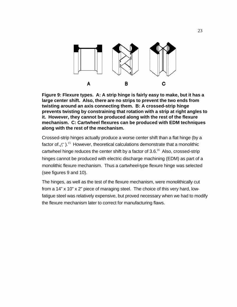
Figure 9: Flexure types. A: A strip hinge is fairly easy to make, but it has a large center shift. Also, there are no strips to prevent the two ends from twisting around an axis connecting them. B: A crossed-strip hinge prevents twisting by constraining that rotation with a strip at right angles to it. However, they cannot be produced along with the rest of the flexure mechanism. C: Cartwheel flexures can be produced with EDM techniques along with the rest of the mechanism.

Crossed-strip hinges actually produce a worse center shift than a flat hinge (by a

factor of 2 ).15 However, theoretical calculations demonstrate that a monolithic

cartwheel hinge reduces the center shift by a factor of 3.6.16 Also, crossed-strip

hinges cannot be produced with electric discharge machining (EDM) as part of a

monolithic flexure mechanism. Thus a cartwheel-type flexure hinge was selected

(see figures 9 and 10).

The hinges, as well as the test of the flexure mechanism, were monolithically cut

from a 14” x 10” x 2” piece of maraging steel. The choice of this very hard, low-

fatigue steel was relatively expensive, but proved necessary when we had to modify

the flexure mechanism later to correct for manufacturing flaws.

24

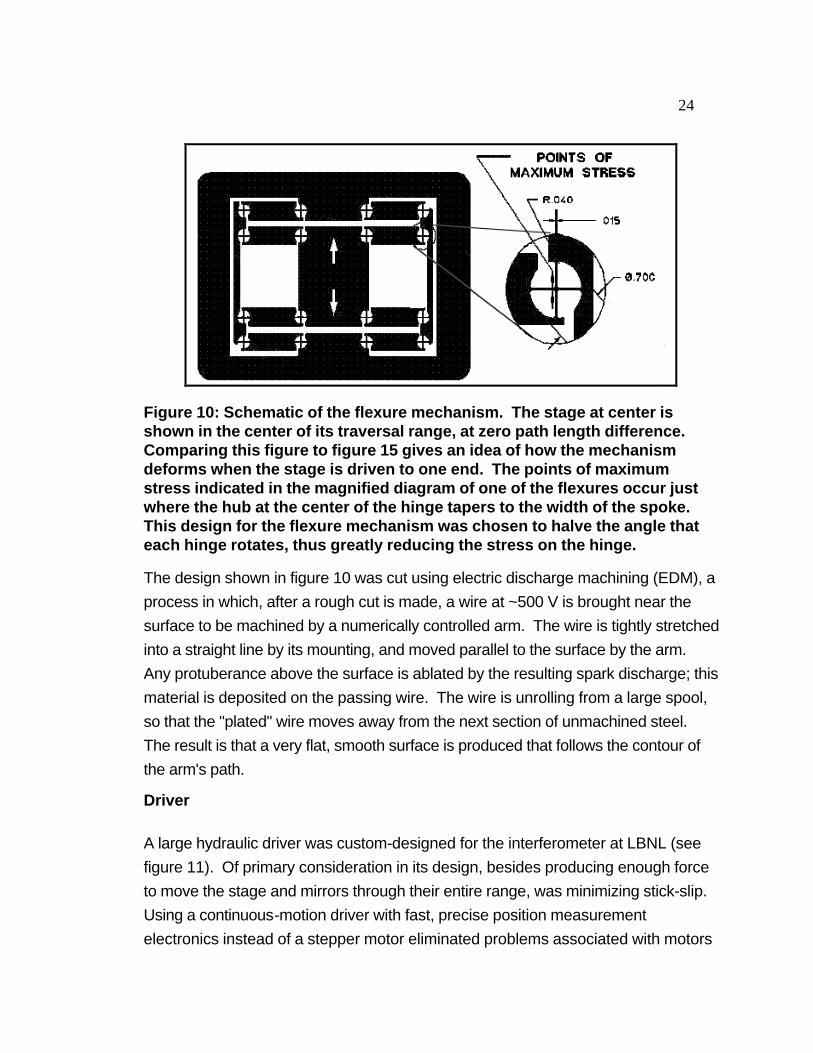
Figure 10: Schematic of the flexure mechanism. The stage at center is shown in the center of its traversal range, at zero path length difference. Comparing this figure to figure 15 gives an idea of how the mechanism deforms when the stage is driven to one end. The points of maximum stress indicated in the magnified diagram of one of the flexures occur just where the hub at the center of the hinge tapers to the width of the spoke. This design for the flexure mechanism was chosen to halve the angle that each hinge rotates, thus greatly reducing the stress on the hinge.

The design shown in figure 10 was cut using electric discharge machining (EDM), a

process in which, after a rough cut is made, a wire at ~500 V is brought near the

surface to be machined by a numerically controlled arm. The wire is tightly stretched

into a straight line by its mounting, and moved parallel to the surface by the arm.

Any protuberance above the surface is ablated by the resulting spark discharge; this

material is deposited on the passing wire. The wire is unrolling from a large spool,

so that the "plated" wire moves away from the next section of unmachined steel.

The result is that a very flat, smooth surface is produced that follows the contour of

the arm's path.

Driver

A large hydraulic driver was custom-designed for the interferometer at LBNL (see

figure 11). Of primary consideration in its design, besides producing enough force

to move the stage and mirrors through their entire range, was minimizing stick-slip.

Using a continuous-motion driver with fast, precise position measurement

electronics instead of a stepper motor eliminated problems associated with motors

25

and gears such as backlash and lead-screw wobble. Errors introduced by these

mechanisms are difficult enough when indexing position at the micron level. They

become nearly intractable at the nanometer level. Piezoelectric materials can

provide repeatable Angstrom-resolution motion, but have a limited range of travel.

The problem of stick-slip will be discussed in detail below, but briefly, it is measured

as a nearly discontinuous "jump" in position while moving the stage at a constant

velocity.

The housing was machined from a solid piece of brass, 8.000" x 4.000" x 4.000",

with a bore diameter of 2.500". The piston was also machined from brass and has

dimensions 2.497" OD and 1.003" ID to accommodate the bore of the housing and

the driveshaft, respectively. It has a 0.184" deep gland (notch for an O-ring) cut in

OD and a 0.184" deep gland cut in ID. The piston is fastened to the driveshaft with

a tapered brass collet. The collet fits into a tapered hole in the piston and both have

matching threaded holes for mating them; screwing them together forces the

tapered collet against the driveshaft.

The driveshaft has several parts to it: a hollow tube, 1.000" OD and 0.750" ID x 17"

that has a 2.5" conflat flange welded to it on one end for bolting it to the vacuum

system via a bellows, an aluminum connecting rod, 0.625" x 24" that has a 1/4-20

threaded hole at either end to accommodate the flexure joints, two stainless steel

flexure joints, 0.625" x 4.05" that have a machined neck, 0.080", allowing for small

angular errors in alignment of the axis of the driveshaft and the center point of the

stage, a taper pin, 0.625" at the large end tapering to 0.500" at the small end for

wedging the collet between the taper pin and the ID of the hollow tube, and a collet,

a piece made from a stainless-steel tube by cutting slits from one end of the tube to

within 1/4" of the other end, alternated with similar ones cut from the other end,

forming a sort of zigzag tube. Screwing in on the taper pin forces the collet against

the ID of the driveshaft, locking the connecting rod to the driveshaft.

26

QuickTime™ and aPhoto - JPEG decompressor

are needed to see this picture.

Figure 11: Schematic of the driver. The piston, housing, and end caps are all made out of brass. A polished stainless steel hollow driveshaft runs through the center of the driver; this is the sliding surface when the piston moves. The driveshaft slides against O-rings at either end of the housing, and is wetted with oil on both sides of the O-ring. Inside the driveshaft , a connecting rod is fastened to one end with a collet; the other end is free. A machined flexure joint between the connecting rod and the collet allows the connecting rod to move about freely within the driveshaft. The other end of the connecting rod is fastened to the flexure stage with another flexure joint, thus allowing small angular movement by the connecting rod without putting a large torque on the stage.

We chose mineral oil as the hydraulic fluid; there are commercial hydraulic fluids

that have better frictional and viscosity characteristics, but mineral oil is readily

available and is good for the skin. The direction and speed of the piston was

controlled by a system of valves, pressure regulator, and Tygon® tubing connected

to ports on either side of the piston. We found the Tygon tubing to be too elastic;

the piston would keep moving after the pressure was released. In the final version

27

of the hydraulic system the Tygon was replaced with rigid copper tubing. Also in the

final version we added solenoid-actuated valves so that spectra could be acquired

completely under computer control.

X-ray Optics

The optics of the interferometer consist of four mirrors and two beamsplitters.

Beamsplitters

Two types of beamsplitters exist: amplitude-dividing and wavefront-dividing. An

example of an amplitude-dividing beamsplitter is the half-silvered mirror used in the

Michelson-Morley experiment to demonstrate the absence of a light wave

propagating ether. The beam must be transmitted through some material such as

glass and either be reflected along one leg of the interferometer or transmitted

along another. However, soft x-rays are quickly absorbed for most materials, so we

selected a wavefront-dividing beamsplitter.

A wavefront-dividing beamsplitter separates a plane wave into a relatively small

number of waves. It consists of a number of alternating slits and flat, mirrored tines

that form a grating. One may get a sense of scale from figure 12. The second

drawing shows a cutaway side view of the beamsplitter. Light would enter from

below at an angle of 20° with respect to the plane of the beamsplitter. Half of the

light would be transmitted through the slits and half would be reflected by the tines.

The rear of the beamsplitter is cut away at a 10° angle to prevent any blocking of the

transmitted beam.

28

This EPS image does not contain a screen preview.

It will print correctly to a PostScript printer.

File Name : bs_1.epsi

Figure 12: Beamsplitter schematic.

Four beamsplitters were each made from a single crystal of silicon by Boeing North

American. Each beamsplitter is a rectangular block of pure silicon, 95.52 mm x

24.00 mm x 5.00 mm (approx. 3 3/4" x 1" x 1/5"). (See figure 12.) The reflecting

surface was ground and polished to a roughness of <5 Å rms and a slope error of

<0.75 µrad rms. The 100 mm period slots were made by using a photolithographic

mask and then anisotropically etching the silicon along the (110) crystalline plane

using KOH as the etchant (see figure 13). Finally, the beamsplitters were coated

with 150Å of molybdenum using vapor deposition, a process that produces

extremely smooth surfaces.17 Molybdenum has one of the highest reflectivities for

x-rays of any known material.18

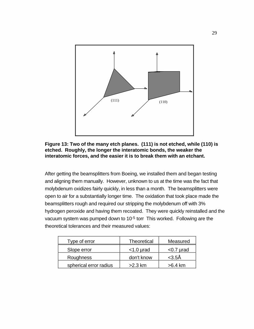
29

(111) (110)

Figure 13: Two of the many etch planes. (111) is not etched, while (110) is etched. Roughly, the longer the interatomic bonds, the weaker the interatomic forces, and the easier it is to break them with an etchant.

After getting the beamsplitters from Boeing, we installed them and began testing

and aligning them manually. However, unknown to us at the time was the fact that

molybdenum oxidizes fairly quickly, in less than a month. The beamsplitters were

open to air for a substantially longer time. The oxidation that took place made the

beamsplitters rough and required our stripping the molybdenum off with 3%

hydrogen peroxide and having them recoated. They were quickly reinstalled and the

vacuum system was pumped down to 10-5 torr This worked. Following are the

theoretical tolerances and their measured values:

Type of error Theoretical Measured

Slope error <1.0 µrad <0.7 µrad

Roughness don't know <3.5Å

spherical error radius >2.3 km >6.4 km

30

Mirror Assembly

A

A'

B'

B

Y

P

P'

Y'

Figure 14: Schematic of the prism used to mount the x-ray mirrors. The vertices of adjacent faces that need to be perpendicular are indicated with the right-angle symbol |_. Thus the faces labeled A, A', B, and B' are all perpendicular to the base. They are also the faces to which the four x-ray mirrors are optically contacted. In addition, opposite faces of the prism must be parallel to each other, so A || A' and B || B'. The face labeled PYY'P' corresponds to the end-on view of side PY illustrated in figure 16, in which the apparatus for measuring the parallelness and perpendicularity of the prism is discussed.

The mirror assembly was made from five separate pieces: four identical

rectangular blocks of glass and a diamond-shaped glass prism. The upper half of

one face of the blocks was initially coated with 500 Å of molybdenum to give them a

mirror finish, but this was later stripped off due to oxidation. The mirrors were then

mounted on the prism by carefully sticking them on its perimeter. No adhesive is

necessary (or desired) if the matching surfaces are flat and smooth enough; The

electrostatic contact forces are strong enough to hold the assembly together.

31

Photon Sciences, the manufacturer of the mirror assembly, qualified it by using

several optical instruments: parallelness and perpendicularity were measured using

an Haidinger fringe test , described below; surface roughness was measured with

a WYKO TOPO 2D surface profiler; slope error was estimated with a WYKO 6000

interferometer and λ/30 test plates.

The Haidinger fringe test exploits the movement of Haidinger fringes to measure the

error in perpendicularity and parallelness of the prism. Haidinger fringes appear as

rings or lines between two nearly parallel surfaces when monochromatic, coherent

light (a laser) is shined normal to the surfaces. The surfaces may bound any

medium (e.g. they may be opposite sides of a block of glass or the faces of two

plates of glass with air between the faces). The fringes arise, of course, from

incident light interfering with light reflected from the downstream surface. The

interference pattern appears at the upstream surface and the image has its focus at

infinity.

If either the observer or the test sample is scanned relative to the other, the fringes

will move; our eyes are sensitive to motion and it is this procedure that is used in

calibrating the prism. One fringe of motion corresponds to an error of λ/4. (The

conditions for maxima and minima are:

d = (m/2 + 1/4)λ/n m = 0,1,2,... maxima

d = mλ/2n m = 0,1,2,... minima

where d is the distance moved, m is the order index of diffracted light, λ is the

wavelength of light, and n is the index of refraction of the glass. These equations

include the 180° phase shift when n2>n1 and 0° phase shift when n2<n1. (n1 and n2

refer to the indices of refraction of the media in which the light is incident and

refracted from the interface, respectively. The two media are air and glass.) If we

plug in the same m in both equations we get �d = λ/4. Glass also amplifies the

sensitivity of the test by shortening the light's wavelength by 1.5, the index of

refraction, and a trained observer can detect motion of 0.1 fringe. Putting all this

together, the minimum observable positional error is λ/40 = 633 nm / (1.5 * 40) = 11

nm.

32

A

LensBS

O

Test Sample

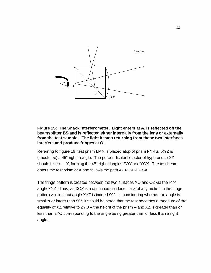
Figure 15: The Shack interferometer. Light enters at A, is reflected off the beamsplitter BS and is reflected either internally from the lens or externally from the test sample. The light beams returning from these two interfaces interfere and produce fringes at O.

Referring to figure 16, test prism LMN is placed atop of prism PYRS. XYZ is

(should be) a 45° right triangle. The perpendicular bisector of hypotenuse XZ

should bisect ∠∠ Y, forming the 45° right triangles ZOY and YOX. The test beam

enters the test prism at A and follows the path A-B-C-D-C-B-A.

The fringe pattern is created between the two surfaces XO and OZ via the roof

angle XYZ. Thus, as XOZ is a continuous surface, lack of any motion in the fringe

pattern verifies that angle XYZ is indeed 90°. In considering whether the angle is

smaller or larger than 90°, it should be noted that the test becomes a measure of the

equality of XZ relative to 2YO -- the height of the prism -- and XZ is greater than or

less than 2YO corresponding to the angle being greater than or less than a right

angle.

33

O

A

D

B

C

X

Y Z

N L

M

P

R

S

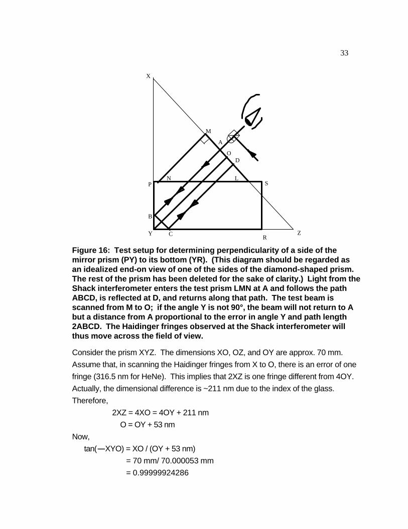
Figure 16: Test setup for determining perpendicularity of a side of the mirror prism (PY) to its bottom (YR). (This diagram should be regarded as an idealized end-on view of one of the sides of the diamond-shaped prism. The rest of the prism has been deleted for the sake of clarity.) Light from the Shack interferometer enters the test prism LMN at A and follows the path ABCD, is reflected at D, and returns along that path. The test beam is scanned from M to O; if the angle Y is not 90°, the beam will not return to A but a distance from A proportional to the error in angle Y and path length 2ABCD. The Haidinger fringes observed at the Shack interferometer will thus move across the field of view.

Consider the prism XYZ. The dimensions XO, OZ, and OY are approx. 70 mm.

Assume that, in scanning the Haidinger fringes from X to O, there is an error of one

fringe (316.5 nm for HeNe). This implies that 2XZ is one fringe different from 4OY.

Actually, the dimensional difference is ~211 nm due to the index of the glass.

Therefore,

2XZ = 4XO = 4OY + 211 nm

O = OY + 53 nm

Now,

tan( ∠∠ XYO) = XO / (OY + 53 nm)

= 70 mm/ 70.000053 mm

= 0.99999924286

34

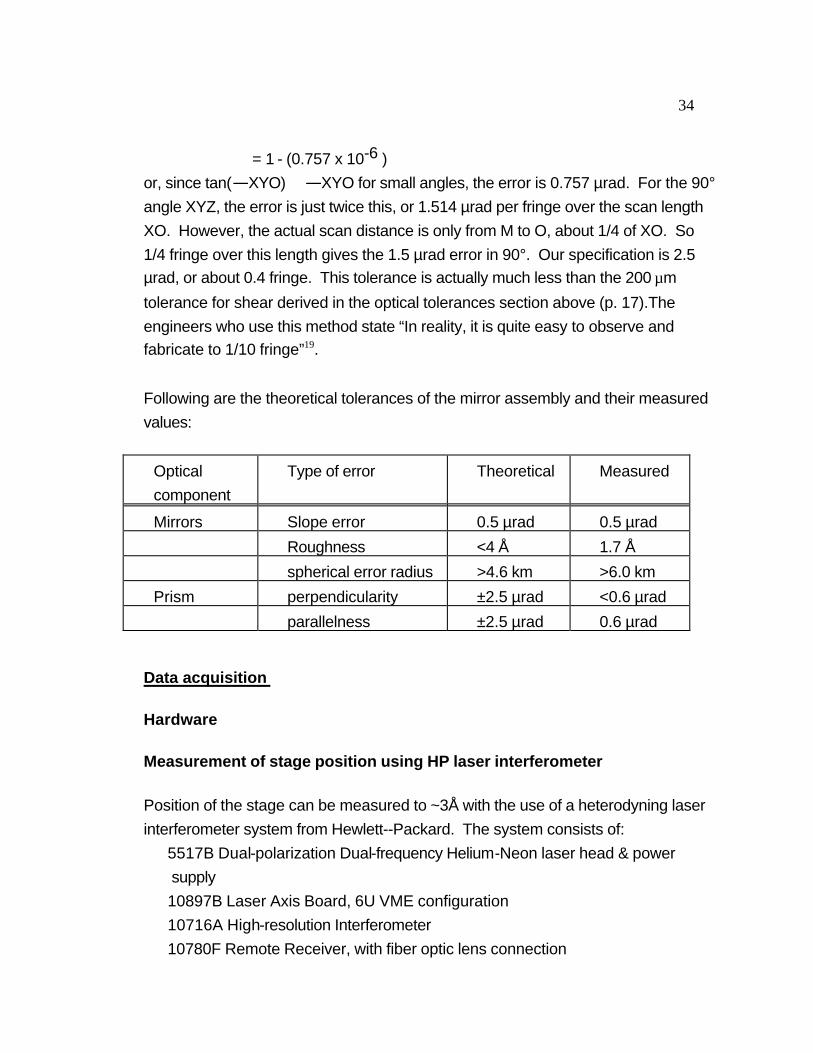
= 1 - (0.757 x 10-6 )

or, since tan( ∠∠ XYO) � ∠∠ XYO for small angles, the error is 0.757 µrad. For the 90°

angle XYZ, the error is just twice this, or 1.514 µrad per fringe over the scan length

XO. However, the actual scan distance is only from M to O, about 1/4 of XO. So

1/4 fringe over this length gives the 1.5 µrad error in 90°. Our specification is 2.5

µrad, or about 0.4 fringe. This tolerance is actually much less than the 200 µm

tolerance for shear derived in the optical tolerances section above (p. 17).The

engineers who use this method state “In reality, it is quite easy to observe and

fabricate to 1/10 fringe”19.

Following are the theoretical tolerances of the mirror assembly and their measured

values:

Optical

component

Type of error Theoretical Measured

Mirrors Slope error 0.5 µrad 0.5 µrad

Roughness <4 Å 1.7 Å

spherical error radius >4.6 km >6.0 km

Prism perpendicularity ±2.5 µrad <0.6 µrad

parallelness ±2.5 µrad 0.6 µrad

Data acquisition

Hardware

Measurement of stage position using HP laser interferometer

Position of the stage can be measured to ~3Å with the use of a heterodyning laser

interferometer system from Hewlett--Packard. The system consists of:

5517B Dual-polarization Dual-frequency Helium-Neon laser head & power

supply

10897B Laser Axis Board, 6U VME configuration

10716A High-resolution Interferometer

10780F Remote Receiver, with fiber optic lens connection

35

We provided the VME crate and controller, and another member of our team (Eddie

Moler) wrote the driver software for the laser positioning system. In addition, we

provided ancillary components: mirror and mirror mount for the stage, mirror and

mirror mount to angle the laser light into the viewport on the side of the vacuum

chamber in which the x-ray interferometer resides, mount for the laser head, and a

mount for the laser interferometer.

Description of HP laser interferometer

The HP laser interferometer measures position to a resolution of ~3 Å in the

following way:20

a. Generate a dual-polarization, dual-frequency laser beam by imposing an axial

magnetic field on the helium-neon gas mixture before excitation. This splits the

energy levels of the light-emitting electrons, and confers opposite circular

polarization on the two slightly different frequencies of emitted light. The engineers

then used waveplates to convert the circularly polarized components into orthogonal

linearly polarized beams.

b. Sample part of the dual-frequency beam within the laser head to create a

reference frequency.

c. Send the rest of the beam to the interferometer, where a polarizing beamsplitter

separates the two frequencies (which are also orthogonally polarized) and sends

them along different paths. One beam hits a retroreflector inside of the

interferometer to provide a non-moving reference beam. The other beam goes to

the mirror on the thing you want to measure. In the high-resolution interferometer,

the measurement beam is reflected four times from the measurement mirror. Since

the path-length difference of the moving and nonmoving beams are doubled for

each pass (once going to the mirror and once coming back), four bounces

multiplies the path-length difference by eight.

d. Recombine the two beams inside of the interferometer and send them to the

receiver, whose detector senses the beat frequency and converts it into a train of

pulses at that frequency.

36

e. Send the reference and measure frequencies on to the Laser Axis Board. Here

the reference waveform is electronically subdivided into 256 equal timeslices. The

edge of the (rectangular) measurement waveform is then binned onto one of the 256

timeslices, thus improving the resolution by 256. This improvement, taken together

with the eightfold improvement due to the multiple passes of the measurement

beam, give a resolution enhancement of 2048. The wavelength of HeNe light is 633

nm, so the resolution is

633 nm/2048 = 0.309 nm.

The position is sampled at a rate of 10 MHz. HP guarantees that the latest datum in

the position register is no older than 0.290 µsec.

Alignment of HP laser interferometer

We mounted the measurement mirror beneath the stage, collinear with the

driveshaft axis. The laser was mounted on a tripod made out of aluminum plate,

threaded rod, nuts, and washers (designed and manufactured by grad students).

We found it necessary to mount another mirror on a magnetic stand in order to

angle the laser light into a viewport on the side of the vacuum chamber. Alignment

then consists of getting the laser beam to go in the top port of the interferometer and

come out the bottom port without hitting the sides. The receiver has a green LED

on it that lights up when it gets a beat frequency. If the alignment is slightly off,

apparently only two of the four passes are traversed by the measurement beam; the

distance measured is half of what it should be. Alignment must be experienced to

be understood.

Measurement of x-ray signal intensity

The x-ray signal is measured in one of two ways: a silicon photodiode or a gas cell

filled with helium under low pressure. The former method measures electrons

liberated from their valence bands by incoming x-rays. The number of electrons,

and therefore the measured current, are proportional to the number of photons and

their energies. Theoretically, the number of electrons liberated is proportional to an

integral multiple of the band gap in silicon, about 3.61 eV. So for 64 eV photons,

37

we would expect 17 electrons and holes to be liberated. (The actual response of

the photodiode depends on a number of things, such as the thickness of any oxide

layer formed on the surface of the diode and impurities.21,22) We used a

Hamamatsu silicon PIN photodiode, model S3580-19.

The photodiode current was amplified and transduced into a voltage with a Keithley

428 Current Amplifier. The output of the amplifier was fed into an analog-to-digital

converter (ADC) board.

Two VME boards, manufactured by Spectrum Communications, are used in

acquisition of the x-ray signals: a carrier board (CV2) for the digital signal

processor (dsp) and a Daughter Module Carrier Board (DMCB) for the analog-to-

digital converter. They are linked externally via the VMEbus backplane and internally

by a 32-bit flat ribbon cable (the dBEX32 bus).

The CV2 provides interfacing between the VMEbus (i.e. the outside world--us), and

the DSP and DMCB. It has shared memory that is available to the VMEbus and the

module that the DSP is mounted on. This module (called TIM after Texas

Instruments Module) has its own local memory and TI's TMS30C40 DSP.

Interfacing to the VMEbus is provided by the VMEbus Interface Control/VMEbus

Address Control (VIC/VAC) chip.

The DMCB can carry up to four modules of various functions. We use one 16-bit

ADC module. The DMCB interfaces its modules with the dBEX32 via AMELIA2

chips, application-specific integrated circuits designed by Spectrum

Communications. The ADC is Burr-Brown's AM/D16SA, a 200 kHz 16-bit

resolution ADC.

Software

Software for the data acquisition system was constructed at three levels: the lowest

level was a program written in C and assembly for the dsp; the middle level was a C

program written for the VMEbus controller that connected the dsp to the Sun

workstation; the top level consisted of a set of LabVIEW panels that controlled

experimental variables and displayed the data. The programs and program

38

environments will be briefly described here; complete descriptions of the dsp and

VxServer programs are included in Appendix 2.

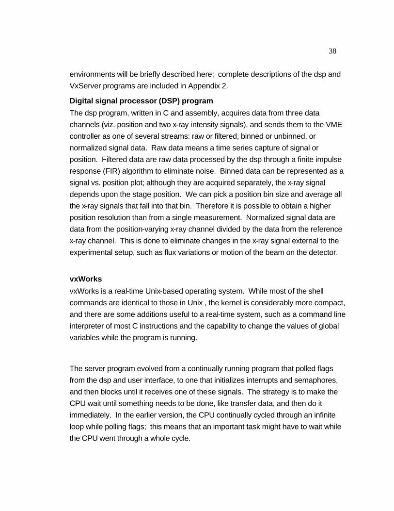
Digital signal processor (DSP) program

The dsp program, written in C and assembly, acquires data from three data

channels (viz. position and two x-ray intensity signals), and sends them to the VME

controller as one of several streams: raw or filtered, binned or unbinned, or

normalized signal data. Raw data means a time series capture of signal or

position. Filtered data are raw data processed by the dsp through a finite impulse

response (FIR) algorithm to eliminate noise. Binned data can be represented as a

signal vs. position plot; although they are acquired separately, the x-ray signal

depends upon the stage position. We can pick a position bin size and average all

the x-ray signals that fall into that bin. Therefore it is possible to obtain a higher

position resolution than from a single measurement. Normalized signal data are

data from the position-varying x-ray channel divided by the data from the reference

x-ray channel. This is done to eliminate changes in the x-ray signal external to the

experimental setup, such as flux variations or motion of the beam on the detector.

vxWorks

vxWorks is a real-time Unix-based operating system. While most of the shell

commands are identical to those in Unix , the kernel is considerably more compact,

and there are some additions useful to a real-time system, such as a command line

interpreter of most C instructions and the capability to change the values of global

variables while the program is running.

The server program evolved from a continually running program that polled flags

from the dsp and user interface, to one that initializes interrupts and semaphores,

and then blocks until it receives one of these signals. The strategy is to make the

CPU wait until something needs to be done, like transfer data, and then do it

immediately. In the earlier version, the CPU continually cycled through an infinite

loop while polling flags; this means that an important task might have to wait while

the CPU went through a whole cycle.

39

VxServer Program Description

In a similar fashion to the dsp program, I will describe the behavior of only one

datastream, "raw signal 1 binned by raw HP position." The main purpose of this

program is to serve as an interface between the dsp program and the user

interface. The user sends a data request from the LabVIEW user interface (running

on a Sun workstation) to VxServer (running on the MVME167 controller, hereinafter

referred to as the 167). Since the two programs reside on different computers, the

request is sent via a Remote Procedure Call (RPC). The source code for this high-

level protocol can be automatically generated by using a Unix function "rpcgen." It is

not described here more than by stating that the RPC task server on the local

machine blocks CPU execution of local functions until it receives a properly

constructed command sent from a remote computer.

Once the RPC for data acquisition is received by s1hpctrl_1, the mirror stage is

moved to the start position, the pertinent parameters for this data stream are set to

their values, and the S1HP flag in the channel_go register is set. The dsp

continuously polls this register, and when it sees the flag immediately starts

collecting data for that data stream.

The dsp sends an interrupt to VxServer when one of its data arrays is filled. The

applicable interrupt handler gives a semaphore (software "interrupt") to other code

that is blocking CPU execution until the semaphore is taken. That code in turn does

whatever processing is necessary and forwards the data array to the user interface

on the Sun workstation.

LabVIEW

LabVIEW is a graphically-based language designed for realtime data acquisition,

processing, and control. The programmer designs a front panel containing controls

40

(e.g. start and stop buttons, numerical and text string entry boxes, and pull-down

menus) and indicators (e.g. "LEDs", numerical and text string outputs, and 2D and

3D graphs, images, and even pictures of incoming data). The guts of the

interactions of the front panel elements are contained in the block diagram

associated with the front panel. Each front panel element created also has an icon

in the block diagram; these block diagram icons may then be "wired" together using

a colored line created by clicking on one icon with a mouse and dragging it to

another icon.

There are many block diagram icons for acquiring, processing, and outputting data.

One may also create icons that interact with object code compiled in other computer

languages. This would be used, for instance, to interface LabVIEW with instrument

drivers that directly acquire data or control motors. We used LabVIEW's networking

VIs to create a Remote Procedure Call (RPC) VI that sends commands to the

vxWorks program, and used Transmission Control Protocol (TCP) VIs to stream the

incoming data to a 2D graph. We also have the option of saving the data to a file or

printing the front panel with its results.

EPICS

The Experimental Physics and Industrial Control System (EPICS) was developed at

Los Alamos National Laboratory as a set of real-time control and data acquisition

tools for particle accelerators. Particularly useful features for the distributed realtime

system that controls the ALS are: the ability to monitor and control machine

variables from any controller (as long as it has permission to do so), broadcasting

the value of any variable to a given list of controllers, and event-driven data flow.

This last feature means that a programmer can set up a block of code to execute

only if a particular variable changes, instead of constantly polling its value (which

wastes valuable CPU time).An experimenter can design a software model of the

way his instrumentation operates using the concept of a state sequencer. For

instance, we needed to initialize certain registers and buffers on our dsp board and

laser axis board, then start data acquisition, and then display the results on a graph.

Using state notation language (SNL, a small subset of the C language, with some

database -specific commands added), we set up the sequence of events; non-SNL

code (i.e. standard C that is not part of SNL) is signified by using the escape

41

character %, and the two software modules are compiled separately and then

linked.

Each database record is a structure comprising a set of fields called process

variables, which are global variables available to the operating system for

monitoring ongoing processes such as data collection, instrumentation status, and

control. Thus we might declare a record called “Power” that is displayed in a

window as a square labeled “ON” when its associated process is active, and

changes to “OFF” if one clicked on it with the mouse; this would inactivate the

process as well. Similarly, we might declare a record called “Data” and monitor its

value; when that value changes, we can plot the new value on a Cartesian display.

Thus the entire program is driven by changes in process variables, which allows for

a much more efficient use of CPU time.

Measurement and rectification of tilt in stage movement

Explanation of problem and data

The purpose of the flexure stage is to move the mirrors in a straight line. While this

may appear to be a simple task, it is one of the most important and demanding

requirements. “Straight” means that the stage must not diverge from a straight line

by an angle of more than 0.5 µrad over its entire range of travel (this tolerance was

derived above in the "Optical Component Tolerances" section above, p. 17). This

requirement dictated the manufacturing tolerances of the flexure mechanism as well

as the optics.

42

QuickTime™ and a

Photo - JPEG decompressor

are needed to see this picture.

Figure 17: Schematic of flexure mechanism, shown deformed. In the lab reference frame, the mirrors move in the ±z direction. The x-ray beam is directed toward the +y direction and is split into two equal components that must remain coplanar through their separate paths, so they can interfere at the other end. Any phase difference must be due only to the linear movement of the mirrors and not to tilt around the y axis (pitch). The stage is shown pushed to the far end of its traversal range. At zero path length difference the stage is centered and the flexures are parallel (see figure 10).

The flexure mechanism may be understood as two pairs of nested rectangles, each

of which may be deformed into a parallelogram. One such pair of rectangles in

figure 17 are ABDC and EFHG. The outer rectangle described by the hinges

ABCD in figure 17 is broken out in figure 18.

43

QuickTime™ and aPhoto - JPEG decompressor

are needed to see this picture.

Figure 18: Schematic for tilt analysis. This is a perspective drawing of the

outer rectangle ABCD in figure 17, above. The stage travels in the ±z

direction. The angles αα and ββ are measured between the axes of two

neighboring hinges (which are supposed to be parallel) in the xy and yz

planes, respectively. In the figure, the two leftmost hinges should both be parallel in the xy plane to the coordinate measuring machine's x-axis. αα 1 is

the angle of the rear axis and αα 2 is the angle of the front axis with the x-axis.

The total angle of these axes relative to each other is αα . Similarly, ββ is the

total angle between the two front hinge axes, measured in the xz plane

parallel to the x-axis. Pitch error would correspond to rotation around the y

axis, and is primarily due to nonzero ββ (see text).

We know from simple beam theory that a cantilever (a stiff but flexible thin rod,

constrained at one end) of length L may be modeled as a couple of length 2L/3 and

a torque centered at the pivot point. This model is valid only for small

displacements of the cantilever from its equilibrium position. A double cantilever

44

(constrained at both ends) may be modeled as two cantilevers whose "free" ends

coincide with the center point between the two constrained ends.

The following analysis follows that of A.E. Hatheway in his paper on the alignment of

flexure stages.23 Hatheway considered a flexure system consisting of two thin

rectangular flexures supporting a rigid rectangular table. He analyzed the effects of

nonparallel neutral axes (nonzero α in figure 18), nonparallel principal axes (nonzero

β in the figure), unequal span lengths, unequal flexure lengths, and driver

misalignments. Of the above possible causes of tilt errors, our design eliminated all

except the first two from contributing significantly to stage pitch for the following

reasons: unequal lengths of the flexures or spans between them produce yaw in our

system; rotation in this direction should not produce deflection of the beams

because the mirrors act as pentaprisms -- if the beam strikes one at a more acute

angle than ideal, it will strike the other mirror at an equally obtuse angle, canceling

the error. Driver misalignments were compensated by adding the flexure joints in

the connecting rod and adding a mechanism for adjusting the push point.

Roll and yaw produce negligible errors, so we consider only pitch error, or rotations around the y-axis (Ry). "Inner" and "outer" rectangles refer to the rectangles EFHG

and ABDC and their analogues MNPO and IJLK on the other side of the stage. The following equations for Ry are taken from Hatheway;24 the values are from our stage.

Nonparallel neutral axes Ry = −3αT z

2

4SL

= α−3(0. 75 cm )2

4(16 .13 cm )( 7. 62 cm ) = -0.00343 α Outer rectangle

= α−3(0.75 cm )2

4(9.98 cm )( 7. 62 cm ) = -0.00555 α Inner rectangle

Nonparallel principal axes: Ry = βT z

S

= β(0. 75 cm )16.13 cm

= 0.0465 β Outer rectangle

= β(0. 75 cm )

9.98 cm = 0.0752 β Inner rectangle

where

45

Ry = pitch angle

α = angle between neutral axes

β = angle between principal axes

Tz = stage travel dis tan ce

2 (stage travel is shared equally

between inner and outer rectangles)

S = span between flexures

L = flexure length

Note that the coefficients for the angles β exceed those of the angles α by about 13

times and are of opposite sign; if the error angles α and β are approximately equal,

then the total pitch will be dominated by error due to nonparallel principal axes, i.e.

β. In fact, the α's were much smaller than the β 's, as shown below.

The error angles α and β are calculated from measurements made by the

Coordinate Measuring Machine (CMM) at LBNL. This instrument can measure

position with a resolution of 3 µm. The flexure mechanism was set on the CMM's

optical table and fiducialized to create a lab reference frame. (Fiducial marks are

reference marks on the flexure mechanism whose positions are known. The rest of

the structures (hinges, beams, frame) are then supposed to have known

coordinates in a Cartesian reference frame, within their respective tolerances.)

Then the positions of the top and bottom of the flexures were compared. The

difference between the two divided by the thickness of the flexure (2.000") gave the

angles α and β.

A worst-case calculation using Hatheway’s theory gives the tolerance for the

machining of the flexure mechanism. Using the case of nonparallel principal axes

for the inner rectangle, we get

46

β =tolerance

2.000"=

Ry

0.0752

or

tolerance =(1 µrad)(2.000" )

0.0752

= 0.00003”

However, the manufacturer could not give us this tolerance. The best he could do

was to offer a tolerance of 0.0003”. When the stage was measured with the CMM,

we found that instead of meeting the requested tolerances of 0.0003", the flexures

were out of tolerance by as much as 0.0035", and instead of the errors being

randomly distributed among the sixteen flexures, the largest errors were in the same

direction along the principal axes.25 When the angles from the CMM

measurements were plugged into the Hatheway model, the calculated pitch agreed

with the measured pitch to within 10%.

Measurement of pitch during stage motion

We used a µ-Radian Instruments MRA-240 autocollimator in making pitch

measurements of the stage. It has a range of three meters and an angular

resolution of 0.1 arcsecond, or about 0.5 µrad. An autocollimator works in much the

same way as the Shack interferometer, described above. Referring to figure 19, a

bright light serves as a source. (Although it need not be either coherent or

monochromatic, it does have to be bright enough to traverse twice the distance

between the beamsplitter and the test surface and interfere at the measuring reticle.

The autocollimator we have uses an ultra-bright LED as its source.) The light is then

transmitted through two condensing lenses that are used to maximize both the

intensity and uniformity of the light directed through the projection reticle in focal plane P1.

47

QuickTime™ and aPhoto - JPEG decompressor

are needed to see this picture.

Figure 19: Autocollimator schematic. Outbound rays are indicated by solid lines, reflected rays by dashed lines. If θθ = 0, the reflected rays would follow the paths of the outbound rays in reverse, reflect from the beamsplitter, and focus on the measuring reticle at x = 0. For θθ � 0, the returning rays focus a distance x = 2θθ fl away. (Schematic courtesy Davidson Optronics.)

The beam is transmitted through the beamsplitter and collimated by the objective

lens. After being reflected by a test mirror, light re-enters the autocollimator and is

focused by the objective lens. The return image appears in sharp focus on the measuring reticle in focal plane P2 after being redirected 90° by the beamsplitter.

Note that since the returning beam is focused by the same optics that collimated it

in the first place, there will not be any dependence of the focal point upon the

distance between the source and the image. The focal plane can be either an

eyepiece or a CCD. The latter is used in our instrument.

If the test mirror has an angle θ with respect to the optical axis, the returning beam will focus at a point on P2 a distance X from the central ray, given by

X = 2θ fL

where fL is the focal length of the objective lens. From the equation it is apparent

that X is independent of the distance between the instrument and the reflecting

surface. X is the centroid of the spot on the CCD.

We used the autocollimator in measuring stage pitch by reflecting its light from the

lower mirror mounted below the stage. (The mirror mount for the stage consists of a

piece of aluminum about 4” x 2” x 1/2”. There are two circular cutouts 1” in diameter,

48

in which two circular mirrors may be mounted. The upper mirror is coaxial with the

driveshaft and the lower mirror sticks down below the stage at the same distance

from the drive axis that the x-ray mirrors are above the axis. Originally, the lower

mirror would have been used with a second laser positioning system to measure

Abbé error, but we decided that was not worth the $15,000 for another laser

positioning system.) The upper mirror was needed for the laser interferometer to

index position. Tilt measurements were made throughout the range of motion of the

stage. We found that the stage tilted by more than 125 µrad over its range, as

compared with the desired pitch of � 0.5 µrad (see p. 17). The tilt was linear with

respect to distance traveled, and was quite reproducible.

Rectification

Discussion of the tilt in light of the Hatheway theory, and considering that the error

angles β were all in the same direction led to a suggestion: could we possibly

correct for the dominant error by introducing a compensating tilt against the β error?

We decided to cut two slits between the frame and hinges (see figure 17). The slits

were cut from the top of the frame to within 1/2" of the bottom, thus providing a hinge

that could be opened up. Holes were drilled at each end of the two slits to

accommodate taper pins. It was the taper pins that would provide the adjustment to

the angular error. They were threaded at one end; as they were screwed in using a

nut, the taper pushed against the upper end of the hole, opening the slit. The tilt was

measured after each careful adjustment. By this method, the tilt of the stage was

reduced from greater than 125 µrad to less than 0.5 µrad rms! The tilt adjustment

has remained stable for over two years.

49

QuickTime™ and aPhoto - JPEG decompressor

are needed to see this picture.

Figure 20: Correction of stage tilt with taper pin adjustment

Blue trace -- underadjustment Red trace -- overadjustment Black trace -- correct adjustment

50

QuickTime™ and aPhoto - JPEG decompressor

are needed to see this picture.

Figure 21: Expanded plot of stage tilt after correction. The pitch error has been reduced to 0.38 µµrad, rms.

Measurement and rectification of vibration and stick-slip

Explanation of problem and data

Mechanical vibrations can be a problem if they produce Abbé errors in the

frequency range of interest (at a stage motion of ~15 µm/sec the x-ray fringes are

coming by the detector at 1 kHz). Stick-slip excites vibrational modes in much the

same way as striking a bell with a hammer excites the bell's harmonics; a square-

like impulse in the time domain transforms into a sum of frequency peaks in the

inverse frequency domain. Solving the stick-slip problem helps greatly in minimizing

the vibration problem.

Abbé error in position measurement is the result of rotation of a rigid body around

the point of measurement. In our case, we want to measure the position of the x-ray

beam. The actual position measurement is made by reflecting laser light from a

mirror whose surface is perpendicular to the axis of motion. The laser beam is

collinear with the driveshaft axis. The x-ray beam strikes the x-ray mirrors about 67

mm above the driveshaft axis, so a pitch angle of 0.5 µrad would produce a position

error of 34 nm. However, a constant error is not a problem; it would be subtracted

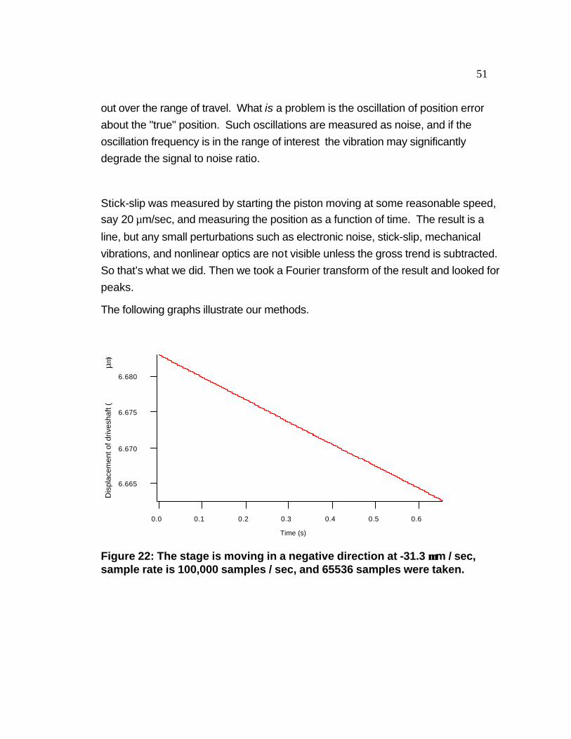
51

out over the range of travel. What is a problem is the oscillation of position error

about the "true" position. Such oscillations are measured as noise, and if the

oscillation frequency is in the range of interest the vibration may significantly

degrade the signal to noise ratio.

Stick-slip was measured by starting the piston moving at some reasonable speed,

say 20 µm/sec, and measuring the position as a function of time. The result is a

line, but any small perturbations such as electronic noise, stick-slip, mechanical

vibrations, and nonlinear optics are not visible unless the gross trend is subtracted.

So that’s what we did. Then we took a Fourier transform of the result and looked for

peaks.

The following graphs illustrate our methods.

6.680

6.675

6.670

6.665

Dis

plac

emen

t of d

rives

haft

(µm

)

0.60.50.40.30.20.10.0

Time (s)

Figure 22: The stage is moving in a negative direction at -31.3 µµm / sec, sample rate is 100,000 samples / sec, and 65536 samples were taken.

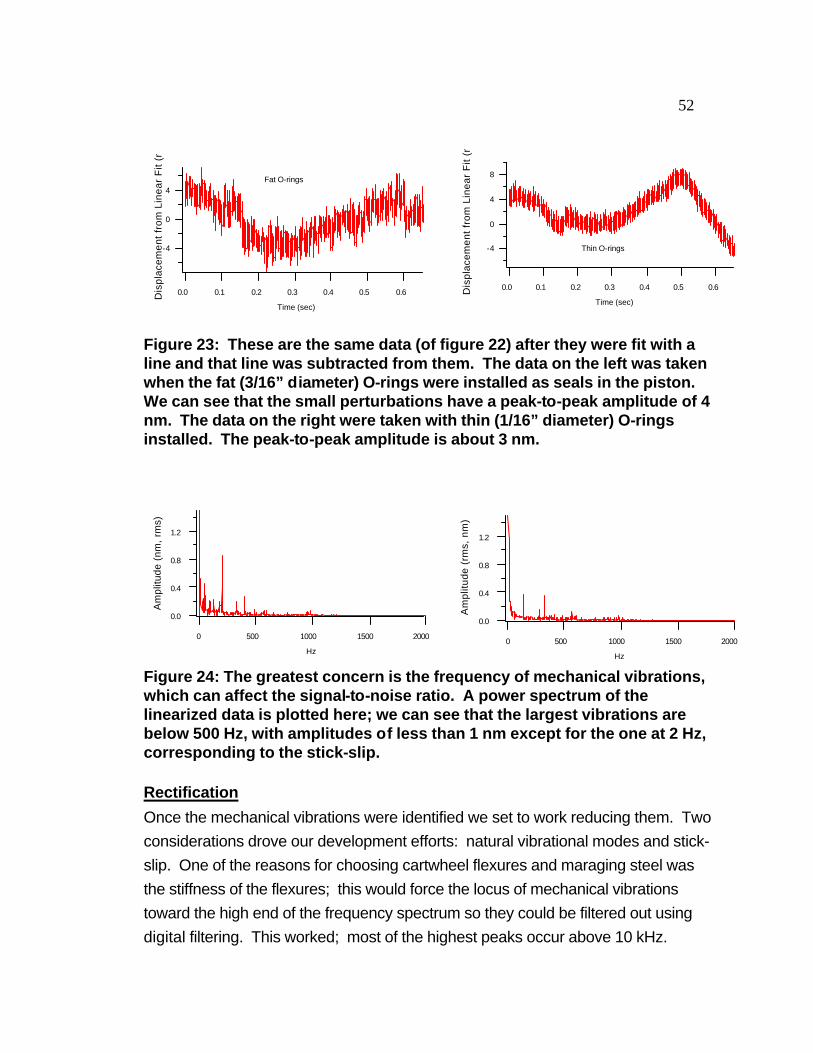
52

8

4

0

-4

Dis

plac

emen

t fro

m L

inea

r F

it (n

m)

0.60.50.40.30.20.10.0

Time (sec)

Thin O-rings-4

0

4

Dis

plac

emen

t fro

m L

inea

r F

it (n

m)

0.60.50.40.30.20.10.0

Time (sec)

Fat O-rings

Figure 23: These are the same data (of figure 22) after they were fit with a line and that line was subtracted from them. The data on the left was taken when the fat (3/16” diameter) O-rings were installed as seals in the piston. We can see that the small perturbations have a peak-to-peak amplitude of 4 nm. The data on the right were taken with thin (1/16” diameter) O-rings installed. The peak-to-peak amplitude is about 3 nm.

1.2

0.8

0.4

0.0

Am

plitu

de (

nm, r

ms)

2000150010005000

Hz

1.2

0.8

0.4

0.0

Am

plitu

de (

rms,

nm

)

2000150010005000

Hz

Figure 24: The greatest concern is the frequency of mechanical vibrations, which can affect the signal-to-noise ratio. A power spectrum of the linearized data is plotted here; we can see that the largest vibrations are below 500 Hz, with amplitudes of less than 1 nm except for the one at 2 Hz, corresponding to the stick-slip.

Rectification

Once the mechanical vibrations were identified we set to work reducing them. Two

considerations drove our development efforts: natural vibrational modes and stick-

slip. One of the reasons for choosing cartwheel flexures and maraging steel was

the stiffness of the flexures; this would force the locus of mechanical vibrations

toward the high end of the frequency spectrum so they could be filtered out using

digital filtering. This worked; most of the highest peaks occur above 10 kHz.

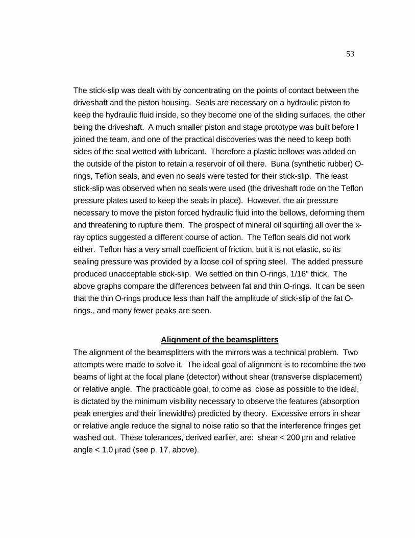
53

The stick-slip was dealt with by concentrating on the points of contact between the

driveshaft and the piston housing. Seals are necessary on a hydraulic piston to

keep the hydraulic fluid inside, so they become one of the sliding surfaces, the other

being the driveshaft. A much smaller piston and stage prototype was built before I

joined the team, and one of the practical discoveries was the need to keep both

sides of the seal wetted with lubricant. Therefore a plastic bellows was added on

the outside of the piston to retain a reservoir of oil there. Buna (synthetic rubber) O-

rings, Teflon seals, and even no seals were tested for their stick-slip. The least

stick-slip was observed when no seals were used (the driveshaft rode on the Teflon

pressure plates used to keep the seals in place). However, the air pressure

necessary to move the piston forced hydraulic fluid into the bellows, deforming them

and threatening to rupture them. The prospect of mineral oil squirting all over the x-

ray optics suggested a different course of action. The Teflon seals did not work

either. Teflon has a very small coefficient of friction, but it is not elastic, so its

sealing pressure was provided by a loose coil of spring steel. The added pressure

produced unacceptable stick-slip. We settled on thin O-rings, 1/16" thick. The

above graphs compare the differences between fat and thin O-rings. It can be seen

that the thin O-rings produce less than half the amplitude of stick-slip of the fat O-

rings., and many fewer peaks are seen.

Alignment of the beamsplitters

The alignment of the beamsplitters with the mirrors was a technical problem. Two

attempts were made to solve it. The ideal goal of alignment is to recombine the two

beams of light at the focal plane (detector) without shear (transverse displacement)

or relative angle. The practicable goal, to come as close as possible to the ideal,

is dictated by the minimum visibility necessary to observe the features (absorption

peak energies and their linewidths) predicted by theory. Excessive errors in shear

or relative angle reduce the signal to noise ratio so that the interference fringes get

washed out. These tolerances, derived earlier, are: shear < 200 µm and relative

angle < 1.0 µrad (see p. 17, above).

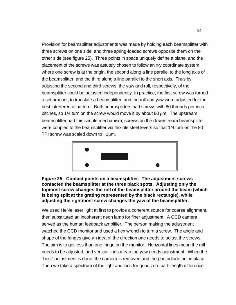
54

Provision for beamsplitter adjustments was made by holding each beamsplitter with

three screws on one side, and three spring-loaded screws opposite them on the

other side (see figure 25). Three points in space uniquely define a plane, and the

placement of the screws was astutely chosen to follow an x-y coordinate system

where one screw is at the origin, the second along a line parallel to the long axis of

the beamsplitter, and the third along a line parallel to the short axis. Thus by

adjusting the second and third screws, the yaw and roll, respectively, of the

beamsplitter could be adjusted independently. In practice, the first screw was turned

a set amount, to translate a beamsplitter, and the roll and yaw were adjusted for the

best interference pattern. Both beamsplitters had screws with 80 threads per inch

pitches, so 1/4 turn on the screw would move it by about 80 µm. The upstream

beamsplitter had this simple mechanism; screws on the downstream beamsplitter

were coupled to the beamsplitter via flexible steel levers so that 1/4 turn on the 80

TPI screw was scaled down to ~1µm.

Figure 25: Contact points on a beamsplitter. The adjustment screws contacted the beamsplitter at the three black spots. Adjusting only the topmost screw changes the roll of the beamsplitter around the beam (which is being split at the grating represented by the black rectangle), while adjusting the rightmost screw changes the yaw of the beamsplitter.

We used HeNe laser light at first to provide a coherent source for coarse alignment,

then substituted an incoherent neon lamp for finer adjustment. A CCD camera

served as the human feedback amplifier. The person making the adjustment

watched the CCD monitor and used a hex wrench to turn a screw. The angle and

shape of the fringes give an idea of the direction one needs to adjust the screws.

The aim is to get less than one fringe on the monitor. Horizontal lines mean the roll

needs to be adjusted, and vertical lines mean the yaw needs adjustment. When the

“best” adjustment is done, the camera is removed and the photodiode put in place.

Then we take a spectrum of the light and look for good zero path length difference

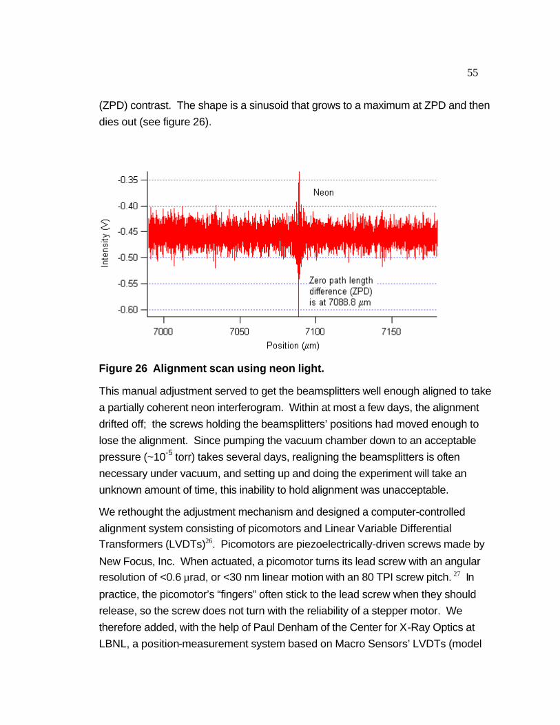
55

(ZPD) contrast. The shape is a sinusoid that grows to a maximum at ZPD and then

dies out (see figure 26).

Figure 26 Alignment scan using neon light.

This manual adjustment served to get the beamsplitters well enough aligned to take

a partially coherent neon interferogram. Within at most a few days, the alignment

drifted off; the screws holding the beamsplitters’ positions had moved enough to

lose the alignment. Since pumping the vacuum chamber down to an acceptable

pressure (~10-5 torr) takes several days, realigning the beamsplitters is often

necessary under vacuum, and setting up and doing the experiment will take an

unknown amount of time, this inability to hold alignment was unacceptable.

We rethought the adjustment mechanism and designed a computer-controlled

alignment system consisting of picomotors and Linear Variable Differential

Transformers (LVDTs)26. Picomotors are piezoelectrically-driven screws made by

New Focus, Inc. When actuated, a picomotor turns its lead screw with an angular

resolution of <0.6 µrad, or <30 nm linear motion with an 80 TPI screw pitch. 27 In

practice, the picomotor’s “fingers” often stick to the lead screw when they should

release, so the screw does not turn with the reliability of a stepper motor. We

therefore added, with the help of Paul Denham of the Center for X-Ray Optics at

LBNL, a position-measurement system based on Macro Sensors’ LVDTs (model

56

no. CD 375-050) and Analog Devices’ AD698 LVDT Signal Conditioner. An LVDT

measures position using three coils along a central axis, and a magnetically

permeable tube within the bore of the coils called the core. The center coil is the

primary winding, and the two coils on either side of it are secondary windings. The

primary is energized with an AC signal, and its resultant magnetic field is coupled to

the secondaries via the movable core. At its null position, the core couples equal

magnetic flux to both secondaries, so the induced potential is zero. If the core

moves closer to secondary #1 than secondary #2, more magnetic flux will be coupled to #1 than #2, and the induced potential V1 > V2. The potential difference

V1 - V2 is then converted to a DC voltage by the signal controller and sent to

Hewlett-Packard’s Data Acquisition/Switch Unit (model no. HP 34970A). This last

instrument has an on-board digital multimeter to read the LVDT voltages, a

switching unit to control the picomotors, and a GPIB interface so we can control it

from our workstation.

This system provided very stable, accurate, and repeatable performance in aligning

the beamsplitters. The system was calibrated with the autocollimator described

above. The LVDTs have a sensitivity of ~300 nm/mV. The coarse adjustment

picomotors have a resolution of 14 µrad on the yaw axis and 40 µrad on the roll

axis. The fine adjustment picomotors (attached to the flexible levers) have a

resolution of 0.21 µrad on the yaw axis and 0.27 µrad on the roll axis. Figure 26

shows an alignment scan using incoherent neon light.

Conclusions

This paper has covered the design and construction of a Fourier transform soft x-ray

interferometer at Lawrence Berkeley National Laboratory. The selection of the

mechanical, optical, and data acquisition subsystems was driven by the

requirements of high energy resolution and coherent recombination of the

separated x-ray beams. In particular, introducing a 2 cm. path length difference

between the separated x-ray beams while maintaining coherence posed technical

problems such as vibration, tilt correction and alignment whose solutions required

experience and careful thought. This was a deceptively difficult instrument to build,

57

and it was possible only with the combined efforts of knowledgeable engineers,

scientists, and technicians.

The interferometer has met its specifications and held them for two years. In itself,

this is quite an accomplishment, given the extremely tight manufacturing tolerances.

It would appear the only thing left to do is to perform the autoionization experiment

for which the instrument was designed. While an interferogram using synchrotron

light has been produced, so far energy peaks have been observed only in the range

of 0 - 10 eV. The scientists now working on the project are following several paths

toward a solution. Among them are:

1. Adding fluorescent detectors throughout the path of the x-ray beam to track its

progress, as an aid in alignment.

2. Replacing the mirror for switching the x-ray beam from the synchrotron to

different endstations. (The other endstations use the beam in a direct line from the

monochromator. Our endstation is th only one that uses the switching mirror, which

could degrade the beam if it is corroded.)

3. Modifying the data acquisition software to take multiple scans and simplify the

filtering of the raw data.

The goal of the interferometer, producing high-resolution double-excitation helium

spectra, has exciting implications in many-body physics, chaos, and electron

correlation theory. The successful conclusion of its construction will be just the

beginning of a long and productive life.

Appendix 1: Derivation of Geometric Factor Used in Calculating Path

Length Difference

The following discussion pertains to movement of the mirrors with respect to the

beamsplitters. In the diagram a mirror whose surface is at line 2 moves along the y

axis to line 2′. Light entering the interferometer is reflected along line 1 at position y01 and again at point P. When the mirror moves to 2′, the light continues to

P′ before it is reflected. Thus the path the light travels before it arrives at center line

C loses distance ∆x and gains distance r.

58

∆X

r

Y

X

2

2'

1

P

P'

BS1

y01

y02

y02'

α

β

Figure A: Path length change due to moving one of the mirrors. The dashed line represents the position of the mirror before moving, the solid line represents the position afterwards. Unprimed variables before, primed after.

The equation for line 1 is y1 = x1 tan α + y01

and for line 2 it is y2 = x2 tan β + y02

Now solve the two equations simultaneously to find the intersection P. yP = (tan α - tan β)x + y01 (A1)

Now if we move line 2 along the y axis to a new position 2′, we get for the

intersection P′

yp' = (tan α - tan β)x′ + y01 (A2)

Subtracting A1 from A2 gives yP' - yP = (tan α - tan β)(x′ - x)

or ∆x =

∆ y

tan α − tan β

59

This ∆x is the magnitude of the path length that is lost when the mirrors move by ∆y.

The magnitude of the path length that is gained by the same motion is gained along

the hypotenuse of the triangle P′PQ, i.e. r is given by (cf. figure A) r = ∆y

1

sin α

and the change in path length by PLD1 = r - ∆x

= ∆y

1

sin α−

1

tan α− tan β

where the subscript 1 indicates that this is the path length change for one leg of the

light path through the interferometer. Referring to figure 4 in the text, we can see

that the total path length difference between the two beams results from the

lengthening of one beam and the shortening of the other beam by the same amount.

Diagram A corresponds to the upper left quadrant of the diagrams in figure 4.

Plugging in the values for our interferometer,

α = 20°, β = 10°, we get PLD1 = 0.342 ∆y

and PLDTOTAL = 4*PLD1 = 1.368 ∆y

Appendix 2: Software Descriptions

Dsp Program (dspacq.c)

The dsp program, written in C and assembly, acquires data from three data

channels (viz. position and two x-ray intensity signals), and sends them to the VME

controller as one of several streams: raw or filtered, binned or unbinned, or

normalized signal data. Raw data means a time series capture of signal or

position. Filtered data are raw data processed by the dsp through a finite impulse

response (FIR) algorithm to eliminate noise. Binned data can be represented as a

signal vs. position plot; although they are acquired separately, the x-ray signal

depends upon the stage position. We can pick a position bin size and average all

the x-ray signals that fall into that bin. Therefore it is possible to obtain a higher

position resolution than that published by the manufacturer. Normalized signal data

are data from the position-varying x-ray channel divided by the data from the

60

reference x-ray channel. This is done to eliminate changes in the x-ray signal

external to the experimental setup, such as flux variations or motion of the beam on

the detector.

The following description pertains to "dspacq.c" as it existed on 11/29/98. I will use

the commenting in that version as section headers for the DSP's setup and

operation. I will not describe variable declarations, allocation of memory, and other

such housekeeping matters. DSP code itself is in boldface; my description is in

normal type.

There are two functions defined in dspacq.c: "main" and "c_int05". "Main" sets up

the various registers on the two VME carrier boards and then enters an infinite while

loop. The while loop is only interrupted by the interrupt service routine (ISR) c_int05.

/* Do Master Cycle in order to be the VMEbus master */

i = Read(VME_CONTROL); /* Save VME master cycle register */

Write(VME_CONTROL, 0X00); /* Set VME master cycle register */

This is necessary to acquire control of the VME bus. VME_CONTROL is a register

in the VMEbus Interface Control (VIC) chip that, as one function, sets the control of

the VME bus to be the VIC chip on the dsp carrier board instead of the VIC chip

on the MVME167.

/********************* C40 stuff *****************************/

/****************** Set up interrupts ************************/

Do_IACK();

This is a macro defined in the header file that sends an "interrupt acknowledged"

signal to

the DSP control register. Since we have not yet started the program running, this

action

61

should not be necessary. However, the state of all hardware registers is undefined

at pro-

gram startup, so they must be initialized to a known state.

set_ivtp(IVTP_DEFAULT);

for(i=0; i<0x40;i++)

*(unsigned int *)(0x2ffe00 + i) = 0;

install_int_vector((void *)c_int05,0x05); /* Set ISR to go when we get an interrupt */

The interrupt vector table (IVT) is a 64-word array in memory containing pointers to

all the

available ISRs. The set_ivtp macro sets up this array at a page boundary, in this

case IVTP_DEFAULT, defined to be a pointer to the location 0x2ffe00. The for

statement zeroes that array, and the install_int_vector macro writes the pointer to

the ISR c_int05 into the interrupt vector table.

/* Set up IIF */

Release_IIOF();

Enable_IIOF_CV2(2, "level"); /* Enable IIOF2 to be level-triggered unlatched interrupt line */

The interrupt flag register (iif) controls the character of the interrupts. There are

three interrupt lines that may be configured as either interrupts or general-purpose

I/O lines. The latter may have such functions as timing, motor control, or anything

else that uses a TTL signal. An interrupt may be either edge-triggered or level-

triggered, and may either be latched into the interrupt flag register until explicitly

released by a command, or released by a read or write of a data register

(unlatched). Here, we first release the Interrupt/Input/Output lines for reconfiguration,

and then set line IIOF2 to be level-triggered, unlatched. This function call also

enables the interrupt.

62

/***********************DMCB stuff ***************************/

The Daughter Module Carrier Board (DMCB) is configured by writing to registers

that are offset from the dBEX32 base address 0xB0000000. The first 64 words are

used to configure the four Application ModulE Link Interface Adapter (AMELIA)

chips that control the four Daughter Module (DM) sites on the DMCB. The next six

words configure six registers that apply to the DMCB as a whole.

.

/* Reset the AMELIA2's on the DM carrier board, then release them */

*DMCB_RESET_REG = 0x0f;

*DMCB_RESET_REG = 0x00;

/* Reset the DM carrier board */

*DMCB_ISR_CTRL = 0;

*DMCB_XRDY_REG = 0;

*DMCB_SYNC_REG = 0;

The above registers are four of the six general purpose register available on the

Daughter Module Carrier Board (DMCB). The 4-bit reset register, as its name

implies, resets the AMELIA2 chips that are mapped into it; the corresponding

AMELIA2 is reset when the bit is set to 1 and then reset to 0. The interrupt control

register (ISR_CTRL) is an 8-bit register used to select which of the three interrupt

lines, XINTA , XINTB , or XINTC , will be used for each daughter module, A, B, C,

or D. Each module is controlled by two of the eight bits; thus setting ISR_CTRL =

0x80 will assign XINTB to daughter module B. The synchronization register allows

a timer on one of the daughter modules (DM) to control the timing on any of the

others. We are using only one DM, so this is set to zero.

/* Configure the DM Site's AMELIA2 (and therefore the DM) */

WriteUL(DMCB_SITE_A + AMELIA_CTR, D16DS_CTR);

63

WriteUL(DMCB_SITE_A + AMELIA_CMR, D16DS_CMR);

WriteUL(DMCB_SITE_A + AMELIA_TMR1, D16DS_TMR1);

The sample frequency of the ADC is set by configuring three registers on the

appropriate AMELIA2 chip. The user must first select the clock source and then

prescale (divide) its frequency by some factor to arrive at the sample frequency.

The User Control Register (CTR) is used to select the clock source and prescale its

input into the Timer 1 (TMR1) register. Two clock frequencies are available from

crystal oscillators on the DMCB: 12.288 MHz (TCLK_0) and 11.2896 MHz

(TCLK_1). Bits 8 and 9 select the clock source: we use TCLK_0. Prescaling

these frequencies to accommodate lower frequency DMs is accomplished by

setting bits 6 and 7. We use a prescaling factor of 1.

The AMELIA Control Register (CMR) is used to configure sixteen control lines

whose functions are determined by what DM is installed. Since the AM/D16SA has

ADC and DAC channels, they can be operated at different frequencies. Bits 4 and

5 of this register select the sample clock for the input (ADC) and output (DAC)

channels. We use the same sample clock for the ADC and DAC, TCLK_0, so

these bits are both set to 1. Bit 7 is used to determine whether the current DM is the

timer master of the other DMs, or a slave to another timer master. This provides

synchronization of sampling. We have only one DM on the DMCB, so our DM is set

as a master.

TMR1 uses the prescaling of CTR to determine the sampling frequency. Its value is

given by the equation

TMR110 = 65537 - F clk

Fs

where Fclk = Frequency of the prescaled selected clock

and FS = Desired sample rate

This register can be set on the fly, and we do so whenever we want to change the

sample frequency. The subtlety here is that TMR1 is an integer, not a floating point

64

number. so the above equation truncates the result of the right side to an integer.

The actual sample frequency is then given by

FS = F clk

65537 − TMR 1

We deal with this detail at the LabVIEW level: when the user inputs a desired

sample frequency, the above calculation is performed and the actual calculated

frequency is displayed for the user's contemplation.

WriteUL(DMCB_SITE_A + AMELIA_CFR, D16DS_CFR);

The configuration register is for configuring the data transfer interface between

AMELIA2 and the DM. The manual did not explain this interface; it merely stated

that the magic value 0x8dff was required to establish valid data communications.

WriteUL(DMCB_SITE_A + AMELIA_IMR, D16DS_IMR);

The interrupt mask register dictates when an interrupt is sent to the C40 via the

dBEX interface. An interrupt may be sent either when an input data register is full

(i.e. an analog-to-digital conversion has been done) or an output data register is

empty (i.e. a digital-to-analog conversion has been done). Setting bits 7 and 14,

respectively, unmasks these two interrupts. We set the interrupt to be sent when an

analog-to-digital conversion has been done.

/* Configure interrupts */

*DMCB_ISR_CTRL |= (XINTB_EN << SEL_SITE_A);

*DMCB_ISR_CTRL |= (NO_INT_EN << SEL_SITE_B);

*DMCB_ISR_CTRL |= (NO_INT_EN << SEL_SITE_C);

*DMCB_ISR_CTRL |= (NO_INT_EN << SEL_SITE_D);

65

Here we set the DMCB interrupt control register to configure interrupts for the four

DM sites; site A is the only one with a DM in it, so interrupt B is enabled for it, and

interrupts are disabled for the other three sites.

/* Clear the FIFOS of invalid data */

d = ReadUL(DMCB_SITE_A + AMELIA_DATA0_IN);

d = ReadUL(DMCB_SITE_A + AMELIA_DATA1_IN);

WriteUL(DMCB_SITE_A + AMELIA_DATA0_OUT, 0X0);

WriteUL(DMCB_SITE_A + AMELIA_DATA1_OUT, 0X0);

The ADC and DAC data registers start out with undefined data in them, so they are

read and written to clear them.

/**************Clear all interrupts *****************************/

/* On DMCB */

d = ReadUL(DMCB_SITE_A + AMELIA_ISR);

Clear the AMELIA2 interrupt service register by reading it.

/* Global Interrupt Enable and Cache Enable */

CACHE_ON();

INT_ENABLE();

Back on the dsp, the last thing we have to do before entering the infinite while loop

that is the usual operating mode, is to enable the instruction cache that holds up to

128 words of past instructions for faster processing, and to globally enable all

interrupts coming into the dsp.

/************ MAIN NON-INTERRUPT LOOP ************/

while(1) {

66

if(++counter1 > 100000)

{TOGGLE(LED3);counter1 = 0;}

There are eight light-emitting diodes on the front panel of the DBV42 carrier board

that the programmer may use for debugging. TOGGLE is a macro that exclusively

ORs the value in the LED register with itself to switch its state. It is used here to

indicate that the non-interrupt loop is running and isn't stuck.

Description of one channel of data

It may be helpful to future experimenters to explain the software by an example how

data is acquired, processed, and sent up the chain of hardware to the user

interface. I will choose the data channel "Raw Signal 1 binned by Raw HP." As the

name denotes, the data in this channel consists of an array of numbers that

represent raw (rather than digitally filtered) measurements of x-ray intensity from the

interferogram detector (rather than the reference detector) that have been averaged

into position bins whose size is set by the user. The position used for each signal

datum is unfiltered data from the HP laser interferometer.

The use of flags is designed to minimize accesses (hits) on the VME bus. The

interrupt service routine and non-interrupt loop run asynchronously, with the ISR

having priority because of its time-critical task, namely taking data from their

registers and putting them in their proper arrays before the next timeout. However,

the non-interrupt loop has the responsibilities of processing the arrays and sending

them on to the 167 before they can be refilled by the ISR. The tasks of the two

blocks are therefore interdependent, so they must communicate with each other via

flags.

Flags are also used to communicate from the program running on the 167,

VxServer, to the dsp program, dspacq. When the latter wants a particular set of

data, it gets the array parameters from the LabVIEW user interface and writes them

into local memory. Then it sets a local flag register whose bits correspond to the

67

data streams that the dsp program can provide. During its initialization, VxServer

has already mapped local memory addresses into VMEbus addresses, so dspacq

knows where the flag registers and data arrays are. (VxServer could also write its

flag register to the dsp, but that produces bus conflicts when the dsp also hits the

VMEbus while doing something else.)

The order in which the flag registers are tested is important; testing registers locally

is faster than across the VMEbus.

One final note: the dsp has two separate buses; local and global. They access

different areas of memory. The ISR fills arrays in one area, sets a flag, and starts

filling the other area. The non-interrupt loop uses DMA to move data from the first

area while the ISR is filling the other one. This is done to prevent bus conflicts on

the dsp. I will describe only the code for the local array; the global array is serviced

by similar code.

/* signal 1 raw binned by HP Raw */

if(S1HPLocalTest == FULL) { /*local buffer is full?*/

Here we test whether the local buffer flag has been set by the ISR (see below).

if(channel_go&S1HP_FLAG) { /* 167 wants more binned signal 1 data */

channel_go is the local copy of the data stream request register that is set by

VxServer in its local memory. This register is read from the 167 in the ISR (see

below). Each bit corresponds to a different data stream. S1HP_FLAG is a mask

for "Signal 1 binned by Raw HP." A TRUE condition means that the 167 wants this

data.

68

if (ReadUL(VME_BASE+S1HP_BFLAG/4)==EMPTY) { /*167 buffer empty? */

This test queries a flag in 167 memory that is set after an array of data has been

written to a file that is accessed by LabVIEW for displaying the data.

S1HPBinSize = 1.0 / Read(VME_BASE + (S1HP_BINSIZE/4));

Get the bin size (i.e. distance in HP steps). Successive bins produce an index into

an array. Each signal datum is acquired simultaneously with a position datum. We

subtract the least position from the current position in the HP position array and

divide the result by the bin size to get the index into the binned signal array. The

current signal datum is then added to the other signal data at that index, and after

the whole array has been thusly binned, the summed value at each index is divided

by the number of points that have been summed to produce an average.

LeastPosLocal = 0xEFFFFFFF;

GreatestBinLocal = 0;

Set the least position in the current position array and the greatest bin index to their

extremes.

/* Find minimum position within safe distance of first position (assume

positions are monotonically increasing)*/

for(i=0;i<SAFE_DIST;i++)

LeastPosLocal =(HPLocal[i] < LeastPosLocal) ? HPLocal[i] :

LeastPosLocal;

69

We use stage position to form an index into the binned signal array. Since arrays

begin with index zero, we look for the least position so that we will always get a

nonnegative number when we subtract it from the current position. We take position

and signal data with the stage traveling only in the positive direction, so successive

positions should form a monotonically increasing series. But the stage jumps

around, and there is mechanical and electrical noise in the system, so we have

picked an arbitrary safe distance from the zeroth position within which the least

position should reside.

/* Bin local signal 1 data*/

for(i=0; i<RAW_ARRAY_SIZE;i++){

Bin = (int)(S1HPBinSize * (HPLocal[i] - LeastPosLocal));

We enter the binning loop and calculate the bin into which we add the i-th signal

datum. The reader may have noticed that when the bin size was read from the 167,

above, that its inverse was calculated. The dsp performs a multiplication faster than

a division, and it is important to maximize the processing speed of operations

performed in loops.

if(Bin < RAW_ARRAY_SIZE && Bin >= 0) {

This condition eliminates glitches (i.e. Bin > RAW_ARRAY_SIZE or Bin < 0).

GreatestBinLocal = (GreatestBinLocal > Bin) ? GreatestBinLocal : Bin;

If the bin size is greater than 1, the binned array will have fewer elements than the

corresponding raw array, so we have to calculate how many points to send on to the

167. This statement will find that number after going through the entire array.

S1HPLocal[Bin] += S1Local[i];

70

++SamplesInS1HPLocal[Bin];

}

Add the current i-th element of the raw signal array to the calculated bin element of

the binned signal array. Increment the integer array that will be used later to

average the signal.

else if(Bin >= RAW_ARRAY_SIZE) {

GreatestBinLocal = RAW_ARRAY_SIZE - 1;

TOGGLE(LED2);

}

else TOGGLE(LED2);

}

Toggle a front panel LED if there are any glitches, but don't include these points in

the binned array.

/* Data averaging for local Signal 1 */

for(i=0; i<= GreatestBinLocal; i++) {

if(SamplesInS1HPLocal[i] == 0)

S1HPLocal[i] = 0;

else S1HPLocal[i] /= SamplesInS1HPLocal[i];

}

Summed data points within each bin are divided by the number of points to get an

average.

Write(VME_BASE + S1HPSTARTPOS_PTR/4, LeastPosLocal);

Write(VME_BASE + GREATESTBIN_PTR/4, GreatestBinLocal);

71

movem((int)S1HPLocal, (int)(VME_BASE + S1PTR/4), GreatestBinLocal+1);

Send the least position in the current array, the number of points, and the x-ray

signal data to 167 memory.

S1HPLocalTest = EMPTY;

for(i=0; i<=GreatestBinLocal; i++) S1HPLocal[i] = SamplesInS1HPLocal[i] = 0;

vmeSetIntStatusID(VICVME_INTLVL,VICVME_INTVEC_S1HP);/* send an interrupt to the vmebus that the buffer is moved*/

vmeSendAsyncInterrupt(VICVME_INTLVL);

Zero flags and buffers. Send an interrupt to the 167 controller to signal it that a

buffer-full of data has been sent.

}

} else S1HPLocalTest = EMPTY;

}

} /*end while(1) */

}/* End of main */

/*************INTERRUPT SERVICE ROUTINE*******************/

int c_int05 (void)

{

unsigned long d;

d = ReadUL(DMCB_SITE_A + AMELIA_ISR);

72

Read the interrupt status register, which must be done to reset the interrupt timer.

Otherwise, the dsp would continually service the ISR and never reenter the infinite

while loop.

/* Acquire data */

if (RawArrayFill==1) {

(Get global position and data points here; the code is similar to that for local data,

described next.)

} else {

HPLocal[index]= HPreg_ptr->pos1_auto_smpl;

S1Local[index] = Read(DMCB_SITE_A + AMELIA_DATA0_IN);

The position datum resides in a 32-bit register on the HP laser axis board. It is

accessed via the VME backplane. X-ray data resides in a 32-bit register in the

AMELIA interface chip. It is accessed via the internal dBEX32 bus.

S1Local[index] <<= 16;/* shift all the way left to preserve the sign bit*/

S1Local[index] >>= 11;/* now drag the sign bit right, but leave 5 bits for resolution improvement */

}

Even though data is sent as 32-bit integers, the ADC provides only a twos-

complement 16-bit integer. We can use the extra 16 bits to improve resolution when

binning the data by left-shifting the data before averaging. The data is then sent to

the 167 as 32-bit integers instead of floating-point numbers. Right-shifting drags

the MSB to the right, so for a signed 16-bit number, we first left-shift by 16 bits to

place the sign bit in the MSB, and then left-shift to drag that bit to the right. The

result is a twos-complement signed 32-bit integer.

73

if(++index == RAW_ARRAY_SIZE) { /* handle full buffer */

channel_go=ReadUL(VME_BASE + CHANNEL_GO_REGISTER/4); /* check which channels are enabled */

A counter (index) is incremented every time the interrupt is serviced (or,

equivalently, every time a data point is acquired). When the index reaches the size

of the raw array buffers, we need to signal the non-interrupt loop that we have a full

array and to start crunching numbers. Also we need to tell the ISR itself that the next

time through it should store the data in the other area of memory. The channel go

register is a bit-mapped flag register residing in controller (i.e. 167) memory. We

set its bits at the 167 level whenever VxServer gets a request for data from the

LabVIEW user interface.

TOGGLE(LED7);

Tell us that the interrupt is being serviced.

WriteUL(DMCB_SITE_A + AMELIA_TMR1, ReadUL(VME_BASE +

ADC_RATE_DIVISOR / 4)); /* update sampling rate */

The procedure for setting the sample rate was described above. Here we read an

address in 167 memory to provide runtime changes to the sample rate.

if(RawArrayFill == 1) { /* finished filling the Global array */

HPGlobalTest=FULL; /* set flags for data processing */

S1GlobalTest=FULL;

S1HPGlobalTest=FULL;

74

The tasks of sending data to 167 memory and binning the data are done during the

non-interrupt routine; this is where we tell the pertinent code blocks that the arrays

are full.

if (HPLocalTest==FULL || S1LocalTest==FULL || S1HPLocalTest==FULL) {

/* buffer overflow! */

TOGGLE(LED6);

vmeSetIntStatusID(VICVME_INTLVL,VICVME_INTVEC_RAWBUFOVFL);

vmeSendAsyncInterrupt(VICVME_INTLVL);

}

After an array of data that must be addressed via the global bus is operated upon

and sent to the 167, its "array full" flag is reset. Here we check whether the

corresponding flag for the local bus has been reset. If it has not been reset, the data

has not yet been sent and will be overwritten by subsequent data. This could

happen if the sample frequency is high and the dsp takes too long to process and

send the data. We send an interrupt to the 167 and toggle a front panel LED to

indicate a problem.

} else {

HPLocalTest=FULL; /* set flags for data processing */

S1LocalTest=FULL;

S1HPLocalTest=FULL;

if (HPGlobalTest==FULL || S1GlobalTest==FULL || S1HPGlobalTest==FULL) {

/* buffer overflow! */

TOGGLE(LED6);

vmeSetIntStatusID(VICVME_INTLVL,VICVME_INTVEC_RAWBUFOVFL);

75

vmeSendAsyncInterrupt(VICVME_INTLVL);

}

Do the same as above for the local bus.

}

RawArrayFill=RawArrayFill^1; /*toggle which array is being filled */

index = 0;

}

}/*end of c_int05*/

VxWorks Program (VxServer.c)

In a similar fashion to the dsp program, I will describe the behavior of only one

datastream, "raw signal 1 binned by raw HP position." The main purpose of this

program is to serve as an interface between the dsp program and the user

interface. The user sends a data request from the LabVIEW user interface (running

on a Sun workstation) to VxServer (running on the MVME167 controller, hereinafter

referred to as the 167). Since the two programs reside on different computers, the

request is sent via a Remote Procedure Call (RPC). The source code for this high-

level protocol can be automatically generated by using a Unix function "rpcgen." It is

not described here more than by stating that the RPC task server on the local

machine blocks CPU execution of local functions until it receives a properly

constructed command sent from a remote computer.

Once the RPC for data acquisition is received by s1hpctrl_1, the mirror stage is

moved to the start position, the pertinent parameters for this data stream are set to

their values, and the S1HP flag in the channel_go register is set. The dsp

continuously polls this register, and when it sees the flag immediately starts

collecting data for that data stream.

76

The dsp sends an interrupt to VxServer when one of its data arrays is filled. The

applicable interrupt handler gives a semaphore (software "interrupt") to other code

that is blocking CPU execution until the semaphore is taken. That code in turn does

whatever processing is necessary and forwards the data array to the user interface

on the Sun workstation.

The following are synopses of the functions in VxServer. The first three are tasks

that are spawned in the vxWorks startup procedure. s1hpctrl_1 and commandctrl_1

are RPCs invoked from the LabVIEW user interface, and S1HP_hndl is the interrupt

handler that services the interrupt from the dsp.

init: initialize the dsp carrier board, get VMEbus addresses for local variables that

the dsp needs to know about and send them to the dsp, configure the error interrupt

handler.

dspacq_run: download the dsp Common Object File Format (COFF) program

and start it running.

s1hpctrl_1: respond to an RPC from the user interface requesting "raw signal 1

binned by raw HP position" by opening binary files for buffering data, allocating

memory, moving the stage to its start position, and setting the channel_go flag that

the dsp monitors for determining which data to collect.

S1HP_run: set up the semaphore and dsp-to-167 interrupt, then go into an infinite

while loop that waits for the semaphore. When it takes a semaphore, S1HP_run

appends the data array to the binary file that the user interface reads. When the

entire data set has been taken the program closes the binary files and frees

memory.

S1HP_hndl: service the interrupt from the dsp indicating the latter has sent a

buffer-full of binned signal 1 data to 167 memory by checking to see whether the

entire set of data has been sent to the user interface. If all the data has been sent,

the channel_go register is reset. Finally, the inter-process semaphore is given to

S1HP_run.

77

commandctrl_1: service RPCs requesting: changes in the sample frequency,

stage position, or global data synchronization.

void init()

{

taskPrioritySet( taskIdSelf(), 125);

vxWorks has a task manager that allocates CPU time in either a round-robin or a

prioritized mode. The programmer can select the mode and priority given to any of

his tasks. Here we give a priority of 125 to the task "init". The highest priority is 0

and the lowest 255.

/*******Initialize DBV42 and TIM modules **************/ if(dbv4xLibInit()!=OK) { printf("dbv4xLibInit failed\n"); exit(-1); }

Initialize library of functions provided by Spectrum Communications for use with their

dsp software.

board=dbv42Create(&desc); if (board==NULL) { printf("dbv42Create failed\n"); exit(-1); }

This function sets up the carrier board.

tim =dbvTIMCreate(board,DBV4x_TIM_SITE_A); if (tim==NULL) { printf("dbvTIMCreate failed\n"); exit(-1); }

78

Make sure tim site A is not already in use.

/* Get VME addresses for several variables and write them to shared memory */ sysBusToLocalAdrs(HP10897A_addrs_type[HP_CARD], HP10897A_addrs_base[HP_CARD],(char **)(&HP_regs_ptr)); /* adc rate divisor */ sysLocalToBusAdrs(VME_AM_EXT_USR_DATA, &adc_rate_divisor,(char**)(&tempintp)); dbv4xWriteSharedWord(board,&tempintp, ADC_RATE_DIVISOR); printf("ADC_RATE_DIVISOR=%d\n",adc_rate_divisor); /* first point of each HP array */ sysLocalToBusAdrs(VME_AM_EXT_USR_DATA, &HPArrayStart,&tempintp); dbv4xWriteSharedWord(board,&tempintp,HP_ARRAY_START); /* first point of each HP array */ sysLocalToBusAdrs(VME_AM_EXT_USR_DATA, &S1HPArrayStart,&tempintp); dbv4xWriteSharedWord(board,&tempintp,S1HP_ARRAY_START); /* number of points in each HP array */ sysLocalToBusAdrs(VME_AM_EXT_USR_DATA, &BinNum,&tempintp); dbv4xWriteSharedWord(board,&tempintp,BINNUM); /* size of position bins */ sysLocalToBusAdrs(VME_AM_EXT_USR_DATA, &BinSize,&tempintp); dbv4xWriteSharedWord(board,&tempintp,BINSIZE); /* channel go reg */ sysLocalToBusAdrs(VME_AM_EXT_USR_DATA, &channel_go_register,&tempintp); dbv4xWriteSharedWord(board,&tempintp,CHANNEL_GO_REGISTER);

The vxWorks operating system has many functions for accessing the VME bus.

Two of them provide mapping of local addresses to VMEbus addresses

(sysLocalToBusAdrs) or vice-versa (sysBusToLocalAdrs). We first declare local

variables that need to be available to a board on the VMEbus, such as the ADC

79

rate divisor. Then the sysLocalToBusAdrs function is executed to get the offset of

that variable's address into the address block that has been set aside for VMEbus

access. Lastly, the mapped address is written to shared memory on the pertinent

VME board. In this case, dbv4xWriteSharedWord is a Spectrum Communications

library call for writing to shared memory on the dsp carrier board. The latter has its

own mapping of the VMEbus and uses the mapped address to write to and read

from the address.

/* setup error-interrupt handler */ intConnect(INUM_TO_IVEC(VICVME_INTVEC_RAWBUFOVFL),RAWBovfl,(int)0); sysIntEnable(VICVME_INTLVL);/*Enable interrupts*/

Here we connect and enable the dsp-to-167 interrupt for dealing with data array

buffer overflows. The RAWBovfl is a pointer to the ISR that handles buffer overflows.

VICVME_INTVEC_RAWBUFOVFL is a one-byte number (= 0xD1) that we defined

in the DSPVME.h header file. The programmer may define up to 256 interrupts for

each of eight interrupt levels. The intConnect function writes the pointer to the ISR

into an interrupt vector table that the CPU looks at whenever it receives an interrupt

of the appropriate level. sysIntEnable then sets a bit in the 167's interrupt service

register that enables the interrupt level VICVME_LEVEL (= 0x04).

printf("End of Init\n"); }

int dspacq_run(void)

{ /* Download the COFF file and Start it running */ if(dbvTIMLoadObject(tim,TIM_FILENAME)!=OK) { printf("dbvTIMLoadObject failed\n");exit(-1); }

This function downloads a 'C40 COFF object file onto a TIM40 site. The entry

address (if any) is remembered for later use.

else if(dbvTIMRun(tim,0)!=OK) {

80

printf("dbvTIMRun failed\n"); printErrno (errnoGet ()); return(ERROR); } else printf("COFF file downloaded and running.\n"); }

This function executes a program on the specified TIM site at the indicated entry

point. If the entry point is 0, then the entry point located in the last COFF module

downloaded to that site is used.

int *s1hpctrl_1(S1HPCommand) bin_command *S1HPCommand; {

This remote procedure is called by the LabVIEW user interface. RPCs are a

standard method designed by Sun Computer for executing functions between two

computers. A port (111) is reserved on all computers using the standard. The

computer acting as the server initiates its RPC service and then blocks (i.e. pauses

CPU execution of the service until it receives a semaphore). The client sends a

request, which consists of a program number, a version number, and a procedure

number, to port 111 of the server. The server unblocks and processes the RPC.

switch(S1HPCommand->execution_state) { case CAPTUREDATA: /* init the data collection */

Here we decide which of the functions within the data channel "Raw Signal 1 binned

by Raw HP position" to perform. There are two; CAPTUREDATA and

ABORTCAPTURE. The former initiates data capture and then turns over control of

data transfer from the DSP to the LabVIEW user interface to an ISR (S1HP_hndl)

that checks whether all the data have been acquired; if they have not, S1HP_hndl

gives a semaphore to the data-forwarding loop in S1HP_run. The latter writes the

data buffer to a file on the Sun workstation, where LabVIEW reads and displays it.

81

S1HP=malloc(RAW_ARRAY_SIZE*sizeof(int)); /* allocate the data buffer */

Allocate memory for the data. Although the actual array will typically be much

smaller than the size of the raw array buffer (the bin size would have to be smaller

than the resolution of the position measurement, ~3Å, for this array to be larger than

the raw array), this size is ample for our purposes.

sysLocalToBusAdrs(VME_AM_EXT_USR_DATA, S1HP,&tempintp); /* tell DSP where buffer is */ dbv4xWriteSharedWord(board,&tempintp,S1HPPTR);

Tell the DSP where the base address of the (local) data buffer is mapped into VME

address space.

ret=0; if (S1HP!=NULL) { /* any errors in allocations? */

Set the return value to zero (i.e. return OK). If things do not work out, this value will

be changed later. Continue with this RPC only if we were able to allocate memory

for the data buffer and open the binary data files. Otherwise, set the buffer pointer to

zero and close the files (see below).

BinSize = S1HPCommand->BinSize/HP_RESOLUTION; S1HPPoints = S1HPCommand->Points; S1HPStart = S1HPCommand->Start; S1HPStop = S1HPCommand->Stop;

The command received from the LabVIEW user interface is an ordered stream of

bytes that we can separate into a structure of variables. Here we assign the

structure members to local variables. This is done to isolate the command structure

from local usage of the variable values: we do not want the values changing

unpredictably in case a new command is sent.

/* go to start position*/ hydro_in(); while((HPArrayStart * HP_RESOLUTION) > S1HPStart - 100.0) {

82

taskDelay(300); printf("Waiting %d sec for start position.....\n", start_time+=5); } hydro_out(); while(S1HPStart > HPArrayStart * HP_RESOLUTION) taskDelay(6);

Move the stage to the start position. The commands "hydro_in" and "hydro_out" are

drivers written by another member of our team (Scott Locklin) for moving the piston

used to drive the stage back and forth. These functions set bits in a Xycom XVME-

240 digital I/O card whose outputs switch solenoid-driven pneumatic valves. This bit

of code moves the stage away from the piston while reading the position every five

seconds, until it is 100 mm past the starting position. The piston then reverses

direction and samples the position at a faster rate (0.1 sec) until it gets back to the

start position. S1HPBflag=EMPTY; channel_go_register_temp |= S1HP_FLAG; printf("S1HPCtrl_1: acquisition initialized...\n"); }

There are two indications to the DSP that we want data on this channel. The

channel_go_register is a bit-mapped 32-bit integer that tells the DSP which of the

twenty possible data streams are wanted. If a particular data stream is requested,

its buffer flag tells the DSP whether the data buffer in 167 memory has been written

to the binary file on the Sun workstation.

else { free(S1HP); printf("S1HPCtrl_1: error allocating data buffer\nAcquisition Aborted!\n"); ret=-1; } break;

If there was an error in allocating memory, this is where we deallocate memory, print

an error message, and return an error value to the calling routine.

83

case ABORTCAPTURE: /* abort data collection */ S1HPPoints=0; printf("Sig 1 Raw binned by HP Raw aborted.\n"); ret = -1; break;

This is the RPC case that aborts data acquisition. It simply sets the number of

points to zero, but as will be seen, this is sufficient to stop data capture and stop the

stage from moving.

default: ret = -1; } return &ret; }/*End of S1HP RPC */

The default case is executed when no other case is. We actually return a pointer to

the return value; this is a part of the RPC convention.

void S1HP_run() {

S1HP_run is the function that does most of the work for this data channel. It waits

for a semaphore that is given by the ISR that responds to an interrupt from the DSP.

The DSP sends the interrupt when it finishes writing a buffer of data to 167 memory.

When S1HP_run receives the semaphore, it writes the data buffer to a binary data

stream that is associated with an Ethernet connection to the LabVIEW user

interface on the Sun workstation.

/* task init */ taskPrioritySet( taskIdSelf(), 105);

Task prioritization is especially important in real-time operating systems. This

means that the programmer can select which running programs - tasks - are more

important than others. These tasks will preferentially receive CPU time when

84

interrupts or semaphores from them are received by the CPU. Priority is a number

from zero to 255, with zero being the highest priority. The highest priorities have

been appropriated by the system executive functions; we wouldn't want the

operating system to stop functioning in order to service on of our tasks; it may not

know how to start again! We have given our highest priority (100) to the port

mapper task; it services RPCs, so we want to be able to send an abort command

via RPC and have that override data acquisition or stage movement. Here we give

a priority of 105 to the operational task for the "Signal 1 binned by Raw HP position"

channel.

/* store pointers to flag into dsp board */ sysLocalToBusAdrs(VME_AM_EXT_USR_DATA, &S1HPBflag,&tempintp); dbv4xWriteSharedWord(board,&tempintp,S1HP_BFLAG);

Get the VME address of the S1HP buffer ready/not ready flag and send that to the

DSP.

/* setup semaphore for buffer filled interrupt message passing */ S1HPbufsem=semBCreate(SEM_Q_PRIORITY,SEM_EMPTY);

Create a binary semaphore that gives a software signal when the 167 CPU

receives a "buffer full" interrupt from the DSP.

/* init the interrupt handler for messages from DBV42 */

/* connect routine to interrupt */

intConnect(INUM_TO_IVEC(VICVME_INTVEC_S1HP),S1HP_hndl,(int)0);

Here we write the pointer to the interrupt service routine to the interrupt vector table;

when the 167 receives an interrupt of a certain level (priority), it goes to the table for

that level and uses the interrupt number to get the pointer to the ISR.

/*always wait for the semaphore then process the buffer */ while(1) { semTake(S1HPbufsem,WAIT_FOREVER);

85

We enter the infinite while loop that is the main operating mode of this task. We

wait for the semaphore given by the DSP ISR after is fills a data buffer.

if(curpts == 0) { /* open the output data file buf */ if((S1HPfd=fopen(S1HP_filename,"a"))==0) printf("Error opening S1HP binary file.\n"); /* open the array parameter file buf */ if((S1HPAPfd=fopen(S1HPAP_filename,"a"))==0) printf("Error opening S1HPAP binary file.\n"); }

Open two files for writing binary data to the LabVIEW user interface on the Sun

workstation. The first file, named S1HP.bin, is used for writing the data buffer. The

second, named S1HPAP.bin, is used for writing the array parameters (viz. number

of points in the variably-sized array and the starting position of the array) used in

correctly indexing the LabVIEW display to the data.

k+=fwrite(&S1HPArrayStart, sizeof(int), 1, S1HPAPfd); k+=fwrite(&BinNum, sizeof(int), 1, S1HPAPfd); if(k == 2){ freopen(S1HPAP_filename, "a", S1HPAPfd); fseek(S1HPAPfd, k, SEEK_SET); }

Write the starting position of the current signal data array and the number of points

to the parameter file. These data are used to correctly place the signal data in the

plot.

j=BinNum; while(j > 0) /* make sure whole buffer gets sent */ j-=fwrite(S1HP+j-BinNum,sizeof(int),j,S1HPfd);

Write the signal data from 167 memory to the data stream buffers.

fflush(S1HPfd); fflush(S1HPAPfd);

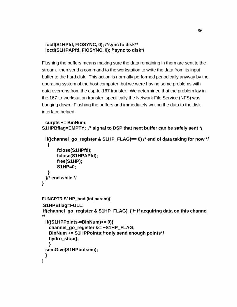
86

ioctl(S1HPfd, FIOSYNC, 0); /*sync to disk*/ ioctl(S1HPAPfd, FIOSYNC, 0); /*sync to disk*/

Flushing the buffers means making sure the data remaining in them are sent to the

stream. then send a command to the workstation to write the data from its input

buffer to the hard disk. This action is normally performed periodically anyway by the

operating system of the host computer, but we were having some problems with

data overruns from the dsp-to-167 transfer. We determined that the problem lay in

the 167-to-workstation transfer, specifically the Network File Service (NFS) was

bogging down. Flushing the buffers and immediately writing the data to the disk

interface helped. curpts += BinNum; S1HPBflag=EMPTY; /* signal to DSP that next buffer can be safely sent */ if((channel_go_register & S1HP_FLAG)== 0) /* end of data taking for now */ { fclose(S1HPfd); fclose(S1HPAPfd); free(S1HP); S1HP=0; } }/* end while */ }

FUNCPTR S1HP_hndl(int param){

S1HPBflag=FULL; if(channel_go_register & S1HP_FLAG) { /* if acquiring data on this channel */ if((S1HPPoints-=BinNum)<= 0){ channel_go_register &= ~S1HP_FLAG; BinNum += S1HPPoints;/*only send enough points*/ hydro_stop(); } semGive(S1HPbufsem); } }

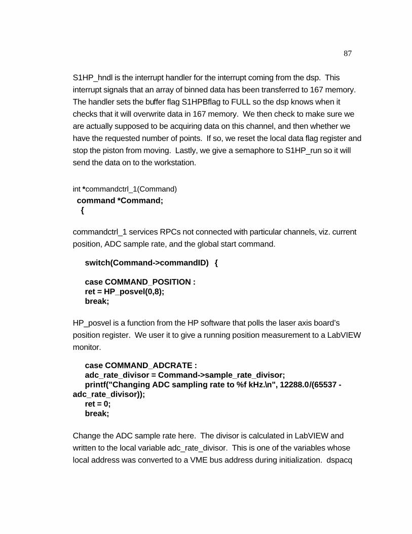
87

S1HP_hndl is the interrupt handler for the interrupt coming from the dsp. This

interrupt signals that an array of binned data has been transferred to 167 memory.

The handler sets the buffer flag S1HPBflag to FULL so the dsp knows when it

checks that it will overwrite data in 167 memory. We then check to make sure we

are actually supposed to be acquiring data on this channel, and then whether we

have the requested number of points. If so, we reset the local data flag register and

stop the piston from moving. Lastly, we give a semaphore to S1HP_run so it will

send the data on to the workstation.

int *commandctrl_1(Command)

command *Command; {

commandctrl_1 services RPCs not connected with particular channels, viz. current

position, ADC sample rate, and the global start command. switch(Command->commandID) { case COMMAND_POSITION : ret = HP_posvel(0,8); break;

HP_posvel is a function from the HP software that polls the laser axis board’s

position register. We user it to give a running position measurement to a LabVIEW

monitor. case COMMAND_ADCRATE : adc_rate_divisor = Command->sample_rate_divisor; printf("Changing ADC sampling rate to %f kHz.\n", 12288.0/(65537 - adc_rate_divisor)); ret = 0; break;

Change the ADC sample rate here. The divisor is calculated in LabVIEW and

written to the local variable adc_rate_divisor. This is one of the variables whose

local address was converted to a VME bus address during initialization. dspacq

88

reads this value whenever the interrupt routine fills an array, and sets the sample

rate accordingly. case COMMAND_GO : channel_go_register |= channel_go_register_temp; /* set channels in temp to acquire */ channel_go_register_temp=0; /* clear temp */ printf("command go issued...\n"); ret = 0; break; default: ret = -1; break; } /* end switch(Command->commandID) */ return &ret; } /* End of Command */

dspacq reads channel_go_register to find out which of the data channels need to be

serviced. channel_go_temp is a local copy not visible to the dsp; its bits are set

separately by the LabVIEW programs for the desired channels of data. The global

start command is sent by Command.vi, and sets the channel_go_register equal to

the accumulated channels in the temporary register. Thus data acquisition is

synchronized for the selected channels.

1R.P. Madden and K. Codling, Phys. Rev. Lett., 10(1963) 516. 2J.W. Cooper, U. Fano and F.Prats, Phys. Rev. Lett., 10(1963) 518. 3 L. Wu and J. Xi, J. Phys. B 23 (1990) 727. 4 A.Macías, T. Martin, A. Riera and M. Yunez, Phys. Rev. A 36 (1987) 4187. 5 M. Domke, K. Schulz, G. Remmers, and G. Kaindl, and D. Wintgen, “High Resolution Study of 1P0 Double-excitation states in Helium”, Phys. Rev A, 53, 1424 (1996). 6 C. D. Lin, Phys. Rev. A 29, 1019 (1984). Much theoretical and experimental work has gone into the physics of autoionization of helium. While this phenomenon will not be dealt with further here, there are several good reviews of the literature, among them the paper by Domke, et. al., cited above, and this one. 7 ibid. 8Huff, W. R. A, PhD Thesis, The University of California, Berkeley, LBL-38492(1996). 9 Chamberlain, J., Chantry, G. W., and Stone, N. W. B., "The Principles of Interferometric Spectroscopy", (Wiley, New York, 1979). 10Howells, M., "Manufacturing Tolerances for the ALS Soft X-ray Interferometer", ALS Note, 5-27-93. 11I. S. Gradshteyn, and I. M. Ryzhik, "Table of integrals, series, and products”, (New York : Academic Press, 1980). 12 M. Born and E. Wolf, Principles of Optics, 7th ed., (Cambridge, Cambridge University Press, 1999), p. 546. 13op. cit., pp. 4-5. 14R. Duarte, M.R, Howells, Z. Hussain, T. Lauritzen, R. McGill, E. Moler, and J. Spring, "A Linear Motion

89

Machine for Soft X-ray Interferometry”, LBNL Report LBNL-40494, July, 1997. 15M.R. Howells, R. Duarte, R. McGill, "Properties of the Cartwheel-type Flexural Hinge", LBNL Report LSBL-213, 1994. 16ibid., p. 6. 17"LBL BEAMSPLITTER QA DATA", Report of quality assurance, Rocketdyne Albuquerque Operations, June 2, 1995. 18The interaction of x-rays with matter is a particular interest of the researchers at the Center for X-ray Optics at LBNL. See, for instance their website at http://www-cxro.lbl.gov. 19 Facsimile communication from David Lunt of Photon Sciences to Malcolm Howells, November 11, 1994. 20 Hewlett-Packard, “Laser and Optics Users Manual”,(HP, Santa Clara, 1992). 21 M. Krumrey, et al., Schottky type photodiodes as detectors in the VUV and soft x-ray range”, Appl. Opt. 27, 4336, (1988). 22 L.R. Canfield, J. Kerner, and R. Korde, “Stability and quantum efficiency performance of silicon photodiode detectors in the far ultraviolet”, Appl. Opt. 28, 3940, (1989). 23Hatheway, A. E., "Alignment of Flexure Stages for Best Rectilinear Performance", SPIE Proceedings, 2542, pp. 70 - 80. 24ibid. 25 The raw CMM data is in a fax from Jerome Cummings to Rob Duarte, July 24, 1995. The analysis was performed by Rob Duarte and described to the author in a telephone call on April 28, 2000. 26 S. Locklin, E. Moler, J. Spring, Z. Hussain, and M. Howells, “Progress in Soft X-ray Fourier Transform Spectrometry”, from “Advanced Light Source Compendium of User Abstracts and Technical Reports 1997”, D. J. Dixon, A. L. Robinson, A. Greiner, and C. Silva, eds., (LBNL, Berkeley, 1998). 27 New Focus’ online information at http://www.newfocus.com/Online_catalog/6/145.