Embed Size (px)
Citation preview
Clemson UniversityTigerPrints
All Theses Theses
12-2010
Design Decisions Under Risk and UncertaintySravya ThoomuClemson University, [email protected]
Follow this and additional works at: https://tigerprints.clemson.edu/all_theses
Part of the Engineering Mechanics Commons
This Thesis is brought to you for free and open access by the Theses at TigerPrints. It has been accepted for inclusion in All Theses by an authorizedadministrator of TigerPrints. For more information, please contact [email protected].
Recommended CitationThoomu, Sravya, "Design Decisions Under Risk and Uncertainty" (2010). All Theses. 970.https://tigerprints.clemson.edu/all_theses/970
DESIGN DECISIONS UNDER RISK AND UNCERTAINTY
A Thesis Presented to
the Graduate School of Clemson University
In Partial Fulfillment of the Requirements for the Degree
Master of Science Mechanical Engineering
by Sravya Thoomu
August 2010
Accepted by: Dr. Georges M. Fadel, Committee Chair
Dr.Mary, E. Kurz Dr.Lonny, L.Thompson.

ii
ABSTRACT
In the contemporary world of engineering, engineers strive towards designing
reliable and robust artifacts while considering and attempting to control
manufacturing costs. In due course they have to deal with some sort of
uncertainty. Many aspects of the design are the result of properties that are
defined within some tolerances, of measurements that are appropriate, and of
circumstances and environmental conditions that are out of their control. This
uncertainty was typically handled by using factors of safety, and resulted in
designs that may have been overly conservative. Therefore, understanding and
handling the uncertainties is critical in improving the design, controlling costs and
optimizing the product. Since the engineers are typically trained to approach
problems systematically, a stepwise procedure which handles uncertainties
efficiently should be of significant benefit.
This thesis revises the literature, defines some terms, then describes such a
stepwise procedure, starting from identifying the sources of uncertainty, to
classifying them, handling these uncertainties, and finally to decision making
under uncertainties and risk. The document elucidates the methodology
introduced by Departments of Mathematical Sciences and Mechanical
Engineering, which considers the after effects of violation of a constraint as a
criterion along with the reliability percentage of a design. The approach
distinguishes between aleatory and epistemic uncertainties, those that can be
assumed to have a certain distribution and those that can only be assumed to be

iii
within some bounds. It also attempts to deal with the computational cost issue by
approximating the risk surface as a function of the epistemic uncertain variables.
The validity of this hypothesis, for this particular problem, is tested by
approximating risk surfaces using various numbers of scenarios.

iv
DEDICATION
To my parents, Venkateswararao and Syamala, and my brother, Akhil Sai.

v
ACKNOWLEDGMENTS
First, I would like to thank to my advisor, Dr. Georges M. Fadel, for his
support, encouragement, and guidance. He has given me academic freedom to
pursue a topic of interest to me and has been extremely supportive throughout
my study. I would like to thank my committee Dr. Kurz and Dr. Thompson for
their support and feedback, and Dr.Wiecek for help.
I would like to extend my thanks to Dr. Sundeep Sampson and Dr.
Santosh Tiwari for their support and guidance during my research. I would like to
thank all the CEDAR lab members for making my stay at Clemson memorable.
I am grateful to the Automotive Research Center for the financial support,
which made me pursue my research without any hurdles. I would also like to
thank the staff of Mechanical Engineering Department at Clemson University for
their help. Last but not the least; I would like to thank all my friends at Clemson
University for their immense support.
vi
TABLE OF CONTENTS
TITLE PAGE .......................................................................................................... i
ABSTRACT ........................................................................................................... ii
DEDICATION ....................................................................................................... iv
ACKNOWLEDGMENTS ....................................................................................... v
TABLE OF CONTENTS ....................................................................................... vi
LIST OF TABLES ................................................................................................. ix
LIST OF FIGURES ............................................................................................... x
1 INTRODUCTION AND LITERATURE REVIEW ............................................ 1
1.1 Uncertainty: .............................................................................................. 2
1.2 Sources of Uncertainty: ........................................................................... 4
1.3 Uncertainty types: .................................................................................... 6
1.3.1 Aleatory Uncertainty: ......................................................................... 7
1.3.2 Epistemic Uncertainty: ....................................................................... 8
1.4 Uncertainty modeling techniques: ............................................................ 9
1.4.1 Fuzzy set theory: ............................................................................. 10
1.4.2 Possibility theory: ............................................................................ 10
1.4.3 Evidence Theory: ............................................................................ 11
1.4.4 Probability theory:............................................................................ 12
1.5 Difference between Uncertainty and Risk: ............................................. 13
1.6 Research Questions: ............................................................................. 17
2 METHODOLOGY ........................................................................................ 20

vii
2.1 Proposed Approach ............................................................................... 21
2.1.1 Level One: ....................................................................................... 22
2.1.2 Level Two: ....................................................................................... 26
2.2 Advantages: ........................................................................................... 29
2.3 Disadvantages: ...................................................................................... 29
2.4 Summary: .............................................................................................. 29
3 CRASHWORTHINESS ................................................................................ 30
3.1 Problem Description: ............................................................................. 31
3.2 Problem formulation: .............................................................................. 35
3.3 Adapting of the problem: ........................................................................ 40
3.3.1 Level 1: ............................................................................................ 40
3.3.2 Level 2: ............................................................................................ 47
3.4 Results: .................................................................................................. 48
4 RISK SURFACE APPROXIMATION ........................................................... 50
4.1 Local Approximations: ........................................................................... 50
4.1.1 Linear Taylor Series Approximation: ............................................... 51
4.1.2 Reciprocal and Hybrid approach: .................................................... 52
4.2 Mid-range Approximations: .................................................................... 53
4.3 Global Approximations: .......................................................................... 53
4.3.1 Response surface Methodology: ..................................................... 54
4.3.2 Kriging: ............................................................................................ 55
4.4 Approach ............................................................................................... 56
viii
4.5 Testing the accuracy of the toolbox ....................................................... 57
4.5.1 Function 1: Rosenbrock function ..................................................... 60
4.5.2 Function 2 ....................................................................................... 61
4.5.3 Function 3 ....................................................................................... 63
4.5.4 Function 4 ....................................................................................... 64
4.5.5 Function 5 ....................................................................................... 66
4.6 Risk surfaces: ........................................................................................ 67
4.6.1 Using 9 scenarios ............................................................................ 69
4.6.2 Using 16 scenarios .......................................................................... 70
4.6.3 Using 25 scenarios .......................................................................... 70
4.6.4 Using 49 scenarios: ......................................................................... 71
4.6.5 Using 169 scenarios: ....................................................................... 71
4.7 Results: .................................................................................................. 72
4.8 Exploring the hypothesis of risk surfaces: .............................................. 76
5 CONCLUSION AND FUTURE WORK ......................................................... 79
APPENDICES ..................................................................................................... 82
References ......................................................................................................... 93

ix
LIST OF TABLES
Table Page
Table 3-1: Classification of Variables .................................................................. 41
Table 3-2: Scenarios ........................................................................................... 42
Table 3-3 : Variable values of scenarios ............................................................. 46
Table 3-4: Results ............................................................................................... 49
Table 4-1: Equations used to test the toolbox ..................................................... 59
Table 4-2: Input data to generate risk surface .................................................... 74
Table 4-3: Results Before approximation ............................................................ 75
Table 4-4: Results after approximation ............................................................... 75
x
LIST OF FIGURES
Figure 1-1: Interdependence of Risk and Uncertainty [34] ...................................... 15
Figure 1-2: Risk Options Example ............................................................................... 16
Figure 2-1: Proposed approach Level One step 1 .................................................... 23
Figure 2-2: Level one step 2 Flow chart ..................................................................... 26
Figure 3-1: Side-impact crash model experimental set up [44] .............................. 32
Figure 3-2: Finite element model of the vehicle [42] ................................................ 33
Figure 3-3: B-pillar [46] .................................................................................................. 35
Figure 3-4 : Response surface equations representing objective and
constraints[43]. ............................................................................................................... 37
Figure 3-5: Response surface equations for objective and constraints of Choi et
al [48]................................................................................................................................ 39
Figure 3-6: Constraint tightening ................................................................................. 45
Figure 4-1: Original Rosenbrock Function ................................................................. 60
Figure 4-2: DACE approximation ................................................................................. 60
Figure 4-3: Actual function ............................................................................................ 61
Figure 4-4: DACE approximation ................................................................................. 62
Figure 4-5: Actual Function........................................................................................... 63
Figure 4-6: DACE Approximation ................................................................................ 63
Figure 4-7: Actual function ............................................................................................ 64
Figure 4-8: DACE Approximation ................................................................................ 65
Figure 4-9: Actual function ............................................................................................ 66

xi
Figure 4-10: DACE Approximation .............................................................................. 66
Figure 4-11: Risk Surface Approximation for 9 scenarios ....................................... 69
Figure 4-12: Risk Surface Approximation for 16 scenarios ..................................... 70
Figure 4-13: Risk Surface Approximation for 25 scenarios ..................................... 70
Figure 4-14: Risk Surface Approximation for 49 scenarios ..................................... 71
Figure 4-15: Risk Surface Approximation for 169 scenarios ................................... 71
Figure 4-16: Approximated Risk Surface showing low risky region ....................... 72
Figure 4-17: Approximated Risk Surface showing low risky region ....................... 73
Figure 4-18: x10 є [-30,30] & x11=0 ............................................................................... 76
Figure 4-19: x10 є [-30, 30] & x11=-30 .......................................................................... 77
Figure 4-20: x10 є [-30, 30] & x11= 30 .......................................................................... 78

1 INTRODUCTION AND LITERATURE REVIEW
In the engineering community, decisions are commonly taken under indefinite
circumstances and the performance of apparently feasible individual alternatives
is not known until the results of these decisions are implemented and used.
Decision making under such circumstances is challenging. These circumstances
are typically called uncertainties in the engineering design community.
Uncertainties affect the design and the function of the systems in many ways. In
the contemporary world, with rapidly growing technologies and global
competition, there is a strong need to understand these uncertainties, their types
and their effects carefully to design and produce products that are globally
competitive. From many decades, significant research in uncertainty has been
on going, and a large amount of literature is available.
When engineers start designing an artifact, they follow a series of steps
known as the certain design process. Before designing a product, a designer
has to ask himself/herself certain questions such as - what is the problem, what
are the product requirements? What are the limitations? What materials and
tools are needed? Who is the customer? What is the goal? She/he has to study
existing technologies and methods that can be used to explore, compare and
analyze many possible ideas and select the most promising idea in order to get a
better output. So, there is a need to collect all the information available that
relates to the problem. However, the presence of uncertainty impacts the final

2
outcome even if a systematic procedure is followed for designing. So engineers
need a step-wise procedure that helps them in handling uncertainties. This not
only helps the novice in knowing the critical as well as trivial details about the
problem but also may result in redefining the problem.
In this framework, the first chapter discusses uncertainty and its definitions by
scholars from different fields; it describes sources of uncertainty and their
significance, uncertainty types, uncertainty modeling techniques, and the
interdependence between risk and uncertainty. The second chapter illustrates
the methodology that was proposed by the researchers at Clemson University.
This methodology introduces a new criterion for decision making and also
elucidates the necessity to handle different uncertainties differently. An
application of this methodology is presented in the third chapter. The fourth
chapter presents an alternative approach that aims to reduce the computation
time in executing the methodology and that may result in a novel interpretation of
risk as a function of certain uncertain variables, and finally chapter five concludes
and proposes possible future extensions to this work.
Having described the motivation for the work and the outline of the thesis, the
next sections expand on the topics of uncertainty and risk, and review the
relevant literature.
1.1 Uncertainty:
The term uncertainty has many lexical meanings. Princeton Word Net [1]
defines it as “Being unsettled or in doubt or dependent on chance” and defines

3
doubt as “The state of being unsure of something”. Merriam Webster [2] defines
it as the things which are vaguely known and are uncontrollable most of the time.
The United States Environmental protection agency [3], EPA, defines uncertainty
as the “Inability to know for sure”. Researchers from fields like economics,
statistics, finance, psychology and engineering have been studying uncertainty
for many years [4, 5]. From the field of economics, Dr. Epstein [5] in “A Definition
of Uncertainty Aversion” defines uncertainty as “General concept that reflects our
lack of sureness about something or someone, ranging from just short of
complete sureness to an almost complete lack of conviction about an outcome”.
In the field of engineering, Klir and Wierman [6] wrote “Uncertainty itself has
many forms and dimensions and may include concepts such as fuzziness or
vagueness, disagreement and conflict, imprecision and non-specificity”. The
authors also mention that “Avoiding uncertainty is rarely possible when dealing
with real world problems. At the empirical level, uncertainty is an inseparable
companion of almost any measurement, resulting from a combination of
inevitable measurement errors and resolution limits of measuring instruments. At
the cognitive level, it emerges from the vagueness and ambiguity inherent in the
natural language. At the social level, uncertainty has even strategic uses and it is
often created and maintained by people for different purposes (privacy, secrecy,
propriety)” [7]. More operational definitions of uncertainty and many researchers’
perspectives towards uncertainty can be found in Hund et al [8] and Dungan et al
[9]. Generally, a researcher’s outlook on uncertainty is related to his or her field

4
of study, and they define the term from the same perspective. However, in
layman’s terms, uncertainty is something which is not known for sure.
Uncertainty is present in every phase of problem solving and decision
making. The sources of uncertainty are numerous. The sources could be lack of
knowledge of the system under study or of its surroundings, variability in input,
unpredictability of the performance of the model under observation, randomness
in the design variables, effect of the environment on the system, etc. The
existence of uncertainty may affect the final outcome of the problem. Identifying
the source of uncertainty and estimating its consequence is a critical task for the
problem solvers and decision makers. Identifying uncertainty and taking
measures to reduce it leads to more reliable and justified decisions. The next
sections explain the sources and the different types of uncertainty.
1.2 Sources of Uncertainty:
In the engineering community, identifying uncertainties and the reason
behind its occurrence helps in understanding their effect on the final outcome
and in taking measures to reduce their consequences. It also helps in identifying
the influential factors and allocating resources accordingly during the process of
designing and decision making. Hence, there is a need to understand the source
of uncertainty before categorizing and handling it. Researches like Moss and
Schneider [10], Klir and Wierman [6, 7] have given their views on the sources of
uncertainty. Moss and Schneider [10] in 2000 classified the sources of
uncertainty as follows.

5
Uncertainties in the input due to:
• Missing components or errors in the data.
• Variability in the data because of imperfect observations.
• Random sampling errors.
• Inaccuracy in measurement.
Uncertainties in models due to:
• unfamiliar functional relationship among the components even if the
functions of individual components are known.
• inherent performance of the system and effects of the surroundings.
• ambiguity in predicting the final outcome.
• qualms introduced by approximation techniques used to solve a set of
equations that characterize some model.
Other sources of uncertainty:
• Vaguely defined concepts and terminology.
• Lack of communication.
Klir and Wierman [6, 7] wrote that the source of uncertainty in any problem-
solving situation is some sort of information deficiency. The authors declare that

6
information could either be incomplete, undependable, or fuzzy, which eventually
leads to uncertainty.
Though there are many sources of uncertainty, as described by researchers from
different fields, the main reasons behind it are:
• Variability
Variability is a characteristic of being subjected to changes. The variation
could be in input, system, or performance of the system, etc.
• Lack of knowledge:
Lack of knowledge about the system, inadequate awareness of
component interactions in a system, insufficient and non reliable
information, contribute for the occurrence of uncertainty.
The next section explains how scholars classify uncertainty into different types
depending on its source.
1.3 Uncertainty types:
Many researchers have categorized uncertainty into different types
depending on the origin of its occurrence. In 1901, Willet [11] categorized
uncertainties into objective and subjective. He illustrated that the happening of an
adverse event can be quantified using probability, which is an objective
uncertainty, while subjective uncertainty results from the lack knowledge and is
non quantifiable. In 1921, Knight [4] subdivided uncertainty into quantifiable and
non quantifiable uncertainties. He explains that the randomness due to

7
quantifiable variability is risk, and the randomness which is due to non-
quantifiable variability is uncertainty. Keynes [12], in 1935, wrote “By uncertainty I
do not mean merely to distinguish what is known for certain from what is only
probable. About these matters there is no scientific basis on which to form any
calculable probability whatever. We simply do not know.” Der Kiureghian [13], in
1989, classified uncertainty into reducible and irreducible. He qualified the
uncertainty that can be reduced by gathering more information or data, which is
currently unavailable, as reducible and the uncertainty that cannot be reduced
due to the nature of unpredictability even though the past data is available, as
irreducible uncertainty.
In the engineering community, commonly distinguished uncertainties in the
literature are aleatory and epistemic [14-16]. Aleatory is a Latin term, which
means “Dependent on chance, luck, or an uncertain outcome” [17]; whereas
epistemic is a Greek word that stands for “of or pertaining to knowledge” [18].
The next section discusses the aleatory and epistemic uncertainties in detail.
1.3.1 Aleatory Uncertainty:
Aleatory uncertainty arises due to the natural variability which cannot be
controlled or predicted. It is also referred as objective uncertainty, stochastic
uncertainty, and irreducible uncertainty [19]. In the field of engineering,
commonly faced aleatory uncertainties are manufacturing uncertainties as
described below.
8
Abramson [20], from the field of engineering seismology describes
aleatory uncertainty as the “natural randomness in a process”. Oberkampf and
Helton [15] used the term aleatory uncertainty to represent the inbuilt variation
associated with a model and its surroundings that are being studied. According to
the authors, the mathematical representations that are usually used to handle
aleatory uncertainties are probability distributions. However, the concern is in the
ease and accuracy of estimating an apt probability distribution for the available
data. When a significant amount of experimental data is available to estimate a
probability distribution, the adequacy of the data could be questionable, but in
general the fit can be obtained. On the other hand, when significant amount of
data is unavailable, obtaining the most suitable fit without any assumptions may
not be practical. The authenticity of speculations could be questioned in such
cases.
Statistical examples of aleatory uncertainty are tossing a coin, throwing a
die, and drawing cards from a pack [21]. Engineering examples are material
properties, dimensions, and unexpected happenings such as component
breakdowns, system malfunctioning, etc.
1.3.2 Epistemic Uncertainty:
Though many designers and decision makers have been dealing with
uncertainty caused due to natural variability and innate randomness, uncertainty
due to lack of knowledge is not considered as extensively as the former.
Researchers define epistemic uncertainty as the uncertainty which arises due to

9
lack of knowledge, or unavailability of data [14-16]. Swiler et al [22] in their
“Epistemic Uncertainty Quantification Tutorial” wrote, “ Epistemic quantities are
sometimes referred to as quantities which have a fixed value in an analysis, but
we do not know that fixed value”. Abramson [20] defines epistemic uncertainty as
“scientific uncertainty in the model of the process due to the lack of knowledge”.
This uncertainty may be reduced to a certain extent by gathering relevant
data and studying the problem thoroughly. However, most of the time it is difficult
to know everything about the problem under study. As an example, consider
temperature on a particular day; it may not be predicted exactly but the two
extremes (low and high) can be forecasted, if past records are available. In the
same manner, the two extremes of snowfall, rainfall, may be forecasted for a
future date well in advance but not the exact quantity. In the next section we will
see techniques that may be used to handle these uncertainties.
1.4 Uncertainty modeling techniques:
Many techniques are proposed by various researchers to handle
uncertainties. Techniques such as Fuzzy set theory, Bayesian probability theory,
Evidence theory or Dempster-Shafer theory, Possibility theory, Interval analysis,
Stochastic modeling with random fields, Monte Carlo simulations, and Multi-
attribute utility theory are some of the popular approaches. Most of these deal
with both aleatory and epistemic uncertainties [23]. Some of these techniques
are illustrated in the following sections.

10
1.4.1 Fuzzy set theory:
The Fuzzy set theory was first proposed by Lotfi Zadeh in 1965 [24-26] as
an extension to conventional set theory. Awareness of fuzzy logic is necessary in
order to understand the fuzzy set theory. In classical set theory, if an element is
present in a set, its membership value is assigned as 1 and if it is not present in
the set, its membership value is assumed to be zero. Fuzzy logic broadens the
concept of classic set theory, such that membership can have a value between 0
and 1. Similarly fuzzy set theory allows partial membership. Uncertainties are
represented using membership values. Assigning membership values is a
commonly faced challenge in this approach. To date, there is no typical rule to
determine the suitability of an assigned membership value [27].
1.4.2 Possibility theory:
Lotfi Zadeh [24-26] first introduced Possibility theory in1978 as an
extension to fuzzy sets; Dubois and Prade [28] continued to develop it [27].
Possibility theory is used when the information on random variations is
inadequate [23]. These variations are handled using possibility distributions.
A possibility distribution is a representation of a set of states of affairs
within a controlled scale like unit interval [0, 1] [28]. The knowledge about the
state helps in distinguishing whether the event is likely to happen or not. If S

11
represents a state of affairs and π represents the mapping from S to a unit
interval [28], the following limits are set:
• Π(S) =0 when the state is impossible [28] .
• Π(S) =1 when the state is truly possible [28] .
One of the limitations of this theory is, if the likelihood of happening of an event is
very small, the theory may suggest that the probability of the event happening is
zero, which may not be a reliable value all the time. However, the majority of the
time, the study of risk and uncertainty deal with events whose probability is less
than 1.
1.4.3 Evidence Theory:
In 1976, Glenn Shafer [29] introduced the Dempster-Shafer theory as an
extension to his advisor, Arthur Dempster’s, work. It is also referred to as
Evidence theory. Evidence theory uses belief and plausibility as measures of
uncertainty [23]. These two measures are obtained from the known evidence
either experimentally or from any other reliable source. Briefly, plausibility of an
event depends on the quantity of belief in the evidence from different sources
about the event. In other words the theory combines the evidences from different
sources and arrives at a degree of belief. For instance, the degree plausibility of
an event “raining” is obtained by gathering information from different sources and
by computing the measure of belief of the sources.

12
1.4.4 Probability theory:
The most commonly used theory to handle uncertainty is probability theory.
According to Merriam Webster [30], the term “probability” is defined “a measure
of how likely it is that some event will occur”. It is based on Kolmogorov’s axioms
[31]. The following are Kolmogorov’s axioms, taken from “Foundations of theory
of probability [31]”.
• Let F be a field of sets.
• Let F contain the set E.
• To each set A in F is assigned a non-negative real number P(A). This
number P(A) is called the probability of the event A.
• P(E) equals to 1.
• If A and B have no element in common, then
( ) ( ) ( )P A B P A P B∪ = +
• If A and B are stochastically independent
( ) ( ) ( )P A B P A P B∩ =
• The conditional probability of event A, given event B, is defined by
( )( | )
( )
P A BP A B
P B
∩=
This theory uses probability, as a measure for uncertainty, which is
computed using previously discussed Kolmogorov’s axioms. When significant
amount of data is available, it is a good method to handle aleatory uncertainty.
Mourelatos and Zhou [32] describe in details the distinction between probability

13
theory, possibility theory and evidence theory in their paper entitled “A Design
Optimization Method Using Evidence Theory”.
These are some of the methods that are used to quantify uncertainties.
After quantifying uncertainties and obtaining the feasible solutions for a problem
one has to choose a better design from among the designs which are
responsible for the feasible solutions. This phase is well known as decision
making phase. In general, during this phase, the selection of a design from
among the available ones is made based on certain criteria like magnitude of
loss or profit, safety, etc. However the criteria are subjective and are connected
to problem under study. In the problems like crashworthiness, majority of the time
(which will be discussed in chapter three) decision are based on the safety and
reliability criteria. In chapter two, a methodology which considers risk of violation
as an additional criterion, along with the reliability and safety, is discussed. But
how is uncertainty quantified when risk is considered as an additional criterion in
design selection during decision making? To answer this question one has to
know the relation between uncertainty and risk, which is presented in the next
section.
1.5 Difference between Uncertainty and Risk:
Another topic of interest for researchers is the interdependence between
risk and uncertainty. Whenever uncertainty exists, risk is associated with it. In the
Risk analysis tutorial [33] the authors write that uncertainty is an intrinsic feature

14
of nature and the effect of uncertainty is the same for all, but risk is specific to a
person. The authors explain it with an example as “The possibility of raining
tomorrow is uncertain for everyone; but the risk of getting wet is specific to one
person”.
In terms of magnitude, uncertainty is the same for all who deal with it, but
risk depends on the choice that a person opts for. The deciding factor is “action”.
Under an uncertain situation, taking an action exclusively depends on the person
who is facing the situation. “Choice” plays a major role in the uncertain
circumstances, which eventually leads to the concept of risk. Where there is a
choice, there is risk most of the times. Profit is the key which pushes a person to
take risk.
In 2008, Samson et al in “A review of different perspectives on uncertainty
and risk and an alternative modeling paradigm” [34] present different perceptions
on uncertainty and risk and their interdependency. According to the authors, in
Knight’s [4] perspective "Uncertainty must be taken in a sense radically distinct
from the familiar notion of Risk, from which it has never been properly
separated.... The essential fact is that 'risk' means in some cases a quantity
susceptible to measurement, while at other times it is something distinctly not of
this character; and there are far-reaching and crucial differences in the bearings
of the phenomena depending on which of the two is really present and
operating.... It will appear that a measurable uncertainty, or 'risk' proper, as we
15
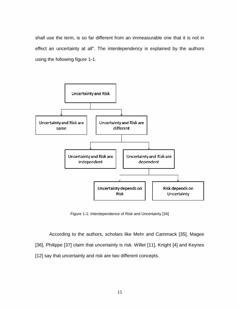
shall use the term, is so far different from an immeasurable one that it is not in
effect an uncertainty at all". The interdependency is explained by the authors
using the following figure 1-1.
Figure 1-1: Interdependence of Risk and Uncertainty [34]
According to the authors, scholars like Mehr and Cammack [35], Magee
[36], Philippe [37] claim that uncertainty is risk. Willet [11], Knight [4] and Keynes
[12] say that uncertainty and risk are two different concepts.

16
People who do not aspire to gain or lose do not act and they are called
non-risk takers or risk avert. People, who expect gain, and act, are called risk
takers. Risk takers and non-risk takers approach problems differently, under the
conditions of uncertainty. Risk takers choose to take an action anticipating gain,
whereas non-risk takers choose not to respond. In the latter case, there may be a
loss of opportunity.
Figure 1-2: Risk Options Example
For example say under an uncertain environment, a group of people is
asked to respond to a situation. Depending on the state of mind of the
participants, they choose to respond or not to respond. People, who do not act,
neither gain nor lose, and thus, do not face any risk. People who choose to act

17
encounter risk; the degree of risk they deal with depends on the alternative they
select. These options are described in figure 1-2. For instance, in a game show
like Ripley’s Believe It or Not, a man chooses to jump from a flying aircraft with
his eyes blindfolded. Assume that the person is unaware of the altitude at which
the aircraft is flying. Anticipating fame he chooses to act and he has only one
alternative to choose from (This is shown in the figure 1-2 under the option single
alternative). Consider a group of people, who has no information about the forest
in which they are lost, and they have to choose a route from three available paths
to make their way to home. The risk of them getting lost in the forest is equally
likely independent of the route taken. (This is shown in the figure1-2 under the
option multiple alternatives). Risk is same for all until a later stage where the
consequences can be known. However the “action” decides it all.
The methodology, which is discussed in chapter two, aids decision makers
in knowing the magnitude of risk for the available alternatives at earlier stages.
This helps them to choose the best design from among the available ones.
1.6 Research Questions:
The motivation behind the research work, which is presented in this thesis,
is raised by studying the different uncertainties, their handling techniques and the
questions that are to be answered for these techniques. Though the distinction
between aleatory and epistemic uncertainties has been explained in the literature
with the help of many examples, still there are many questions about their
classification. For instance, consider a highway whose geometry is known; can

18
we predict the occurrence of an accident on the route by knowing the previous
data? Does the knowledge about the number of previous accidents help in
reducing the uncertainty?
The motivation leads to following questions:
Question 1: How and depending on what are uncertainties classified?
In extension to the first research question, we can try to better understand the
aspect of uncertainty and ask ourselves the following question:
Question 2: How can one know whether the available information is
adequate or not?
In engineering optimization problems, with all the requirements and
constraints that are to be satisfied, finding feasible designs is a complicated task.
The next equally complicated and may be even more demanding task is Decision
Making. During the phase of decision making, generally a design which performs
best most of the time over all the feasible designs is chosen.
Question 3: Is it the percentage of dependability alone that decides the
design selection or should the decision makers consider some additional criteria
to make the selection more trustworthy?
Question 4: How are criteria considered in design selection?
In order to answer the first three questions, it is necessary to understand
problem by knowing its fundamental characteristics. One has to be aware of
possible uncertainties that could be encountered in the context of engineering

19
design. The answer for the fourth question can be found in the following
chapters.
As mentioned earlier the next chapter explains the methodology that was
developed by the researchers at Clemson University, which introduces an
additional criterion for decision making and also elucidates the necessity to
handle different uncertainties differently.

20
2 METHODOLOGY
Deterministic optimal solutions are accurate only when there is no
randomness or uncertainty associated with either design variables or system
performance, system or its performance. Often, the results obtained by
deterministic methods are very useful, yet deterministic methods are used to
obtain possible optima without considering uncertainties. However, if there are
ways to deal with uncertainties the results should be more accurate and useful.
The methodology discussed in this chapter addresses specifically the latter point.
In the engineering community, typically encountered uncertainties are due
to the imprecision, inaccuracy in measurement or in the models, unexpected
system performance, or uncontrollable factors such as climatic conditions. The
most common reasons behind the uncertainty are manufacturing variability and
randomness in system behavior. During the manufacturing phase, a dimension
may not be attained to the desired level of accuracy in every case. However, it
can be obtained within some tolerance range. If sufficient data can be obtained
from the manufacturer, this variability can be handled by using appropriate
probability distributions and methods that consider uncertainty.
Several such methods are proposed in the literature. Most of these
methods consider the reliability of the designs as a criterion in choosing the
better design among the available designs. Rockafellar [38], in one of his articles
in 2007 raised objections to these methods. One of his main concerns is the risk

21
of violation of constraint. The argument is; two designs, one which is reliable 95
times and the other 90 times out of hundred times, are considered. In choosing a
design from among them, one would opt for the design which is more reliable.
But, what are the effects when the most reliable design fails? What are the
effects when the less reliable design fails? The first design may have worse
effects when it fails than the second design, even though it is more reliable.
Therefore, when choosing a design, the after effects of a potential failure should
also be considered.
2.1 Proposed Approach
Addressing this issue, the Departments of Mechanical engineering and
Mathematical sciences at Clemson University have combined their efforts to
come up with an approach. This approach not only considers the reliability of a
design but also considers the after effects of its violation during the design
selection process. A clear distinction is maintained between aleatory and
epistemic uncertainties, and a new way to handle epistemic uncertainty is also
introduced with this approach. No distributions are assumed for the epistemic
uncertain variables in this methodology unlike the conventional methodologies
that handle uncertainties. The proposed approach consists of two levels. The first
level finds the reliable designs for all possible combinations of discrete epistemic
uncertainties. The second level helps in finding the least risky design which
performs best over the whole range of epistemic uncertainties. The following

22
sections explain the approach in detail, describing each level and the steps within
these levels.
2.1.1 Level One:
Level one has two steps. In the first step, the problem of interest is
completely studied and the variables that are to be optimized are recognized.
These design variables are sorted out into aleatory and epistemic uncertain
variables. Once the categorization is done, each epistemic uncertain variable is
divided into discrete values. All possible combinations are made out of these
discretized epistemic uncertain values and each combination is called a scenario.
For instance, say e1, e2… en are epistemic uncertainties variables and a1,
a2… an are aleatory uncertain variables. Each epistemic uncertain variable is
divided into p discrete values within some acceptable bounds. Assume that e1
can take values from 10 to 50, it is divided into “p ” discrete values. If p =5, then
e11 =10, e12 =20, e13 =30, e14 =40, and e15 =50 is a possible discretization of e1.
The higher the value of p is, the more the problem gets computationally
expensive. For n epistemic uncertain variables, each divided into p steps there
will be p n combinations i.e., p n scenarios.
2.1.1.1 STEP 1
1. Categorize the design variables

23
a. Epistemic uncertain design variables (e1, e2, e3…..)
b. Aleatory uncertain design variables (a1, a2, a3…..)
2. Discretize each epistemic uncertain variable.
3. Each discretized combination of these uncertainties is called a Scenario
(S1, S2, S3…..).
Figure 2-1: Proposed approach Level One step 1

24
2.1.1.2 STEP 2
In the second step, a deterministic optimum for all the aleatory uncertain
variables is calculated at each scenario and the obtained deterministic solution is
populated within their allowable tolerance range. Each design that is generated is
checked to verify if it satisfies all the constraints or not and a feasibility
percentage of each constraint is computed by dividing the number of feasible
designs over the total number of designs generated. Identify the constraint which
has least feasibility percentage among all the constraints. Tighten this constraint
by a predefined step size and find a new solution which satisfies this constraint.
Repeat the process until all the designs generated satisfy each and every
constraint at least up to preferred feasibility percent. The preferred feasibility
percent is chosen by the decision maker. The following explains step 2
algorithmically.
1. Find the deterministic optimum at each scenario.
2. Determine the tolerance range by finding the distance from the
deterministic optimum to the variable bound.
Range = [deterministic solution – tolerance, deterministic solution +
tolerance]
3. Generate ‘n’ number of random designs based on the distribution of the
aleatory uncertain variables values within the above mentioned range.
4. Check whether each design is feasible with respect to all constraint. In
order to calculate the feasibility percentage of each constraint, count the

25
number of feasible designs N feas and divide it by the total number of
designs generated.
Feasibility Percentage = Total number of designs generated
feasN
5. Set the desired reliability percentage (R) (Eg. R=90, 95, 99, etc).
6. Find the constraint which is most critical (lowest reliability). Tighten the
constraint by a predefined step size and find a new design which satisfies
this constraint.
7. Repeat the process until each constraint’s feasibility percentage becomes
either greater or equal to desired reliability percentage (R).
8. Save the design which satisfies all the constraints and under its respective
scenarios. These designs are here on referred as reliable designs.

26
Figure 2-2: Level one step 2 Flow chart
2.1.2 Level Two:
After obtaining reliable designs for every scenario in the first level, in level two
evaluate how good a scenario’s reliable design works at other scenarios. In other
words calculate the risk of a scenario’s reliable design at all the other scenarios.
In order to compute this, generate deigns within the limits of each aleatory

27
uncertain variable as done in level one step 2 and find the reliability percentage
of each constraint. While doing this, keep track of the amount by which a
scenario’s design is violating the constraint at other scenarios and calculate the
mean (this takes care of the after affects of violation). Divide the calculated mean
by the reliability percent of a constraint. If the reliability percentage of a constraint
is hundred, there is no risk because it is reliable all the time. If the reliability
percentage is in between zero and hundred, the risk is the mean violation over
the reliability percentage of the constraint. If the reliability percentage is zero, it
means the design violates the constraint at that particular scenario all the time.
Dividing the mean by zero must be avoided, so for mathematical purposes
whenever the reliability percentage is zero, the mean is divided by a very small
finite number (penalty number). Finally the design which is least risky is chosen.
The approach is explained algorithmically as follows:
• For each reliable design di evaluate the satisfaction of safety constraints
( )ki jr z with respect to all the other scenarios jz
• Calculate the risk of each reliable design di with respect to the violation of
each safety constraint.
( ) prob( ( , ) 0) for all i,jki j k i jr z g d z= ≤

28
kµ : Mean violation of safety constraints
γ : Penalty number (e.g., 0.0001)
( )ki jr S : Risk of constraint k at scenario j
If the number of constraints is k and number of scenarios is j then the total
number of risk vectors is j and the total number of elements in each risk vector is
k x j. If there exists a risk vector whose k elements are all smaller than all the
elements of the rest of risk vectors then the risk vector is called a non-dominated
risk vector and the respective scenario and design is chosen to be the least risky
design. If such vector doesn’t exist, then a vector of zero risk is assumed to be a
ideal vector and the proximity of the risk vector to the ideal risk vector is
computed using l 2 –norm. l 2 –norm is also called as Euclidean norm [39]. (For
detailed information on l 2 –norm refer “Matrix analysis” by Horn and
Johnson[40]). Finally, the vector which is closest to the zero risk vector is chosen
to be the least risky design.
• Choose the least-risky design based on the proposed approach
0 ( ) 1
/ ( ) 0 ( ) 1
/ ( ) 0
ki j
k k ki j ki j
k ki j
r z
risk r z r z
r z
µµ γ
=
= < < =

29
2.2 Advantages:
The advantages of the approach are the following
1 It considers the effects of the failure of a design along with the reliability.
2 It handles epistemic uncertainties without assuming any distributions.
3 It avoids the selection of the worst case scenario design.
4 It does not restrict aleatory uncertain variables to just normal distribution.
5 It considers both percentage of reliability and risk after violation as criterion in
the design selection.
2.3 Disadvantages:
The method could be computationally expensive for more number of
epistemic variables and finer discretization, yet with the available number of high
performance computers managing this, might not be extremely difficult.
2.4 Summary:
Having described the proposed approach, the next chapter considers the
crashworthiness problem, applies the procedure to identify least risky designs
and discusses the results.

30
3 CRASHWORTHINESS
Crashworthiness is defined as “A measure of the vehicle’s structural ability
to plastically deform yet maintain a sufficient survival space for its occupants in
crashes” in Vehicle Protection and Occupant Safety [41]. In more general words,
it is the ability of a vehicle to protect its occupants by withstanding an impact. The
common types of crashes result from the impact on the side, rear, or front of a
vehicle or due to rollover. A newly designed vehicle is released to the market
only when it satisfies all the safety regulations that are mandatory in the
respective country [42]. Due to the global competition, automotive engineers are
inclined towards designing safer as well as lighter vehicles. It is an arduous task
to achieve because these two characteristics are contradictory. If the vehicle has
to be safer it has to be stronger, strength is typically correlated with structural
weight. Furthermore because of the push to become more energy efficient,
vehicles should be lighter to consume less fuel. In designing vehicle structures
that satisfy these criteria, aspects like possible impact locations, and uncertainty
in these locations, safety rules and regulations, and material and structural
properties should be carefully considered.

31
3.1 Problem Description:
One example that considers three aspects: lightweight, structural and
occupant safety, and uncertainty, is the side impact crash worthiness problem
that was proposed by Gu and Yang [42, 43]. Figure 3-1 shows the physical
experimental set up of a side-impact crash test. The objective of this side-impact
crashworthiness problem is to minimize the weight of the vehicle structure
subject to structural and safety constraints.
During the experiment, a deformable barrier travelling at 31mph hits the
vehicle structure. The collision with the vehicle structure occurs within a
predefined distance from a selected point. For example, the barrier hitting height
can be within δ distance above or below the pre-determined point and the barrier
hitting position can be anywhere within δ to the left or to the right of the pre-
determined point. The δ chosen by the authors for this problem is 30mm. The
rationale behind the selection of the pre-determined point could be: the point
being a critical point and the deviation from this point may be sufficient to provide
some measure of the performance of the vehicle in a crash. In more general
terms, if the selected impact point is at coordinates (0,0), the hitting height and
hitting position can be within a range of -δ to δ from the impact point.

32
Figure 3-1: Side-impact crash model experimental set up [44]
However, it is too expensive to conduct the crash tests physically in order
to get substantial amount of data that can be used to quantify the uncertainties.
Yet to get an estimate about the vehicle’s capability, a dummy that replicates the
behavior of a human body is placed inside the car model and a crash test is
conducted in general and then softwares are used to simulate the data obtained
for further results. While conducting the crash test, certain guidelines are to be
followed. Because the problem under study is a side-impact crash problem, side-
impact safety guidelines are followed. The most commonly followed side impact
safety guidelines are those of the US National Highway Traffic Safety
Administration and of the United Nations Economic Commission for Europe. The
31 mph 31 mph 31 mph

33
Euro-New Car Assessment Program (Euro-NCAP) [45] side impact test rules
were followed for this problem by the original authors of the study.
Figure 3-2: Finite element model of the vehicle [42]
Since the repeated physical crash tests are expensive to conduct, the
problem is formulated as an optimization problem and the finite element model,
shown in figure 3-2, was used by Gu and Yang [42, 43] to obtain response
surfaces, in the form of equations, for the objective and constraints. The finite
element dummy model consists of around 90,000 shell elements and 96,000
nodes. The design variables that are to be optimized are the following
dimensions of structural members: B-pillar inner (x1), B-pillar reinforcement (x2),
floor side inner (x3), cross member (x4), door beam (x5), door belt line (x6), roof
rail (x7), and the material properties of the B-pillar inner (x8), and the of floor side
34
inner (x9). In addition, there are two non-design parameters: the barrier hitting
height (x10) and the barrier hitting position(x11). The design variables x1 through
x7 are material thicknesses that are continuous, whereas x8 and x9 are material
properties. The material properties are discrete variables which either takes the
value of the yield strength of mild steel or that of high strength steel. The authors
treated the safety criteria (that are to be satisfied according to EURO-NCAP side-
impact procedure), as constraints. Such an approach enables researchers to use
approximate, but inexpensive simulations in terms of computer time to reach
some optimum.
The safety constraints are the force that effects the abdomen (abdomen
load, Al), the chest injury caused by the deformation of soft tissues due to the
sudden change in velocity measured at three different locations (upper, middle,
and lower) on the torso called the viscous criterion (VCu, VCm, VCl), the upper,
middle and lower rib deflections (RDu, RDm, RDl ) and the possible tear in the
cartilage connecting the left and right pubic bone (pubic symphysis force, F). The
structural responses are the velocity of the B-pillar at its middle point and the
front door velocity at the B-pillar. In addition, two more constraints: the velocity of
the B-Pillar at its middle point and the velocity of the front door at the B-Pillar
were also considered. The B-pillar is the vertical metal support linking the front
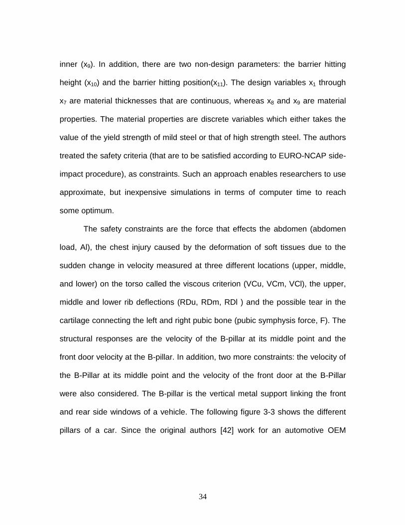
and rear side windows of a vehicle. The following figure 3-3 shows the different
pillars of a car. Since the original authors [42] work for an automotive OEM

35
company (Ford) they may have wanted additional safety criteria and considered
these two constraints in the problem they describe in the literature.
Figure 3-3: B-pillar [46]
The following is the mathematical representation of the problem, where
the objective is to minimize the weight subject to safety and structural
constraints.
3.2 Problem formulation:
Minimize Weight of the vehicle structure
Subject to Abdomen Load ≤ 1.0 KN
Viscous Criteria ≤ 0.32 m/s

36
Upper Rib Deflection ≤ 32 mm
Middle Rib Deflection ≤ 32 mm
Lower Rib Deflection ≤ 32 mm
Pubic Symphysis Force ≤ 4.0 KN
Velocity of B-pillar at middle point ≤ 9.9mm/ms
Velocity of front door at B-pillar ≤ 15.70 mm/ms
In the process of creating response surfaces for the objective and
constraints, the optimal Latin hypercube sampling [47] was chosen to generate
the points. The authors state that they used 3N to 4N (where N is total number of
design variables) number of points to obtain a relatively accurate response
surface. A quadratic stepwise regression method was used by the authors [42] to
create these response surfaces which are shown below in the figure 3-4.

37
Figure 3-4 : Response surface equations representing objective and constraints[43].
In 2004, Youn and Choi [48, 49] used a finite element car model that
consists of 85,941 shell elements and 96,122 nodes to study the uncertainties.
This is also a side-impact crash test. No changes were made with respect to the
initial velocity of the barrier that hits the vehicle structure, which remains at 31
mph. The safety regulation procedure that was used is also the European
Enhanced Vehicle-Safety Committee (EEVC) [50] procedure. The problem
formulation remains the same as the original problem with the objective being the
minimization of structural weight subject to the same structural and safety
constraints.

38
Minimize Weight
Subject to Abdomen Load ≤ 1.0 KN
Viscous Criteria ≤ 0.32 m/s
Upper Rib Deflection ≤ 32 mm
Middle Rib Deflection ≤ 32 mm
Lower Rib Deflection ≤ 32 mm
Pubic Symphysis Force ≤ 4.0 KN
Velocity of B-pillar at middle point ≤ 9.9mm/ms
Velocity of front door at B-pillar ≤ 15.70 mm/ms
With the same design variables the Latin Hypercube Sampling (LHS)
combined with quadratic backward stepwise regression [51] method was used to
generate response surfaces. 3N data points were generated using LHS in order
to get an accurate response surface; N being the number of variables (design as
well as non design) [42, 43]. Yet, the response surfaces are different from the
former ones either in the decimal places of coefficients of the interactive terms or
in the interactive terms itself. The response surfaces generated are:

39
1 2 3 4 5 7
2 4 2 10 3 9 6 10
2 1 8 3 10
3 10
= 1.98 + 4.9 + 6.67 + 6.98 + 4.01 + 1.78 + 2.73
1.16 0.3717 0.00931 0.484 0.01342
46.36 9.9 12.9 0.1107
33.86 2.95 0.1792 5.05
Weight x x x x x x
Subject to
Al x x x x x x x x
RDl x x x x x
RDm x x
= − − − +
= − − +
= + + − 1 2 2 8 5 10 7 8 8 9
3 1 2 5 10 6 9 7 8 9 10
1 2 1 8 2 7 3 5 5 10 6 9
7 11.0 0.0215 9.98 22.0
28.98 3.818 4.2 0.0207 6.63 7.7 0.32
0.261 0.0159 0.188 0.019 0.0144 0.0008757 0.080445
0.0
x x x x x x x x x x
RDu x x x x x x x x x x x
VCu x x x x x x x x x x x x
− − − +
= + − + + − +
= − − − + + +
+ 8 11 10 11
5 1 8 1 9 2 6 2 7 3 8 3 9
5 6 5 10 6 10 8 11
2 3 8
0138 0.00001575
0.214 0.00817 0.131 0.0704 0.03099 0.018 0.0208 0.121
0.00364 0.0007715 0.0005354 0.00121
0.74 0.61 0.163
x x x x
VCm x x x x x x x x x x x x x
x x x x x x x x
VCl x x x
+
= + − − + − + +
− + − +
= − − + 23 10 7 9 2
24 2 3 4 10 6 10 11
1 2 2 8 3 10 4 10 6 10
3 7 5 6 9 10
0.001232 0.166 0.227
4.72 0.5 0.19 0.0122 0.009325 0.000191
10.58 0.674 1.95 0.02054 0.0198 0.028
16.45 0.489 0.843 0.0432 0.05
x x x x x
F x x x x x x x x
Vb x x x x x x x x x x
Vf x x x x x x
− +
= − − − + +
= − − + − +
= − − + − 29 11 1156 0.000786x x x−
Figure 3-5: Response surface equations for objective and constraints of Choi et al [48].
Where Al stands for Abdomen load, RDl, RDm, RDu for Rib deflection
lower, middle and upper; VCu, VCm, VCl stand for viscous criterion upper,
middle and lower; F for Pubic symphysis force. However, both side-impact
crashworthiness problems have become bench mark problems to study different
types of optimization techniques and different types of uncertainties.

40
3.3 Adapting of the problem:
3.3.1 Level 1:
Step1:
The response surfaces (in the form of equations) formulated by Dr.Youn
[49] are used for our study. The authors modeled all the variables x1 to x11 as
aleatory uncertain variables. However, in our case, because of the nature of the
variables and their variability, design variables x1 through x7 are categorized as
aleatory uncertain variables and x10 and x11 as epistemic uncertain variables.
Since it is obvious that x8 and x9 can take either the value of mild steel or high
strength steel it is clear that there is no uncertainty associated with these two
variables beyond possible uncertainty in material properties. However, in the
present study, that uncertainty is not considered. The following table 3-1 shows
the classification of the design variables.

41
Variable Uncertainty Type Lower bound Upper bound Distribution Standard deviation
x1 Aleatory 0.5 1.5 Normal 0.03
x2 Aleatory 0.5 1.5 Normal 0.03
x3 Aleatory 0.5 1.5 Normal 0.03
x4 Aleatory 0.5 1.5 Normal 0.03
x5 Aleatory 0.5 1.5 Normal 0.03
x6 Aleatory 0.5 1.5 Normal 0.03
x7 Aleatory 0.5 1.5 Normal 0.03
x8 Either 0.192 (Mild Steel) or 0.345 (High Strength Steel)
x9 Either 0.192 (Mild Steel) or 0.345 (High Strength Steel)
x10
Epistemic -30 30 - -
x11
Epistemic -30 30 - -
Table 3-1: Classification of Variables
The methodology that is proposed in chapter two is applied to the side-impact
crashworthiness problem. Here, the epistemic uncertain variables x10 and x11 are
discretized into five values within the range -30 to 30. Each combination is called
a scenario. So there are twenty five scenarios in this particular problem. The
following table shows all the scenarios (S1, S2 … S25).

42
Table 3-2: Scenarios
As mentioned in chapter two, the proposed methodology is a two level
methodology. Step 2 in level one is illustrated in the following section.
Step 2:
For each scenario Si (i=1,2,…..25), the following optimization problem is solved.
Minimize Weight
Subject to Abdomen Load ≤ 1.0 KN
Viscous Criteria ≤ 0.32 m/s
Upper Rib Deflection ≤ 32 mm
Middle Rib Deflection ≤ 32 mm
Lower Rib Deflection ≤ 32 mm
Pubic Symphysis Force ≤ 4.0 KN
Velocity of B-pillar at middle point ≤ 9.9mm/ms
Velocity of front door at B-pillar ≤ 15.70 mm/ms

43
1 2 3 7 , , , .. [0.5 1.5]x x x x… ∈
8 9, x x is either 0.192 or 0.345
The obtained solution for the variables x1 through x9 for a scenario i is
referred scenario i’s design.
3.3.1.1 Calculating the reliability percentage of a constraint:
Reliability:
Reliability is defined in Merriam-Webster Dictionary [52] as “The extent to which
an experiment, test, or measuring procedure yields the same results on repeated
trials”. In other words, reliability is a measure of the ability of a system or design
to achieve the same results independently of the allowable variability in the
design variables.
Reliability percentage:
In this thesis, the reliability percentage is taken to be the number of times a
system or a design achieves the desired outcome out of hundred tries with
various allowable values of the design variable. Such a quantification of reliability
may be used as a percentage, and is in line with common specifications of
reliability (99% reliable, 99.7% reliable or 3Sigma, 6sigma, etc.).
3.3.1.2 Calculating the reliability percentage of a constraint:
Considering the solution of the aleatory variables as mean, the aleatory uncertain
variables are distributed normally with a standard deviation of 0.03. Later on, N

44
random designs are generated for all aleatory uncertain variables within their
respective bounds. (N is a arbitrary value for this problem it is 10000). Each
random design is tested for its feasibility with respect to each constraint. For a
constraint, the ratio of the number of feasible random designs (Nfeas) to the total
number of random designs (N) is called the reliability percentage of that
particular constraint.
Reliability percentage of a constraint Rc =
feasN
N
3.3.1.3 Desired Reliability Percentage
The reliability percentage that is to be achieved is assumed to be the three
sigma range (99.87%) for this particular problem. It is named the desired
reliability percentage (R).
The process consists in finding the constraint which has the least reliability
percentage out of all the constraints, and tightening that constraint by a
predefined step size. The step size is determined by the difference between R
and Rc. If that difference is greater than 5, the step size is set to be 0.01 times
the right hand side of the constraint or else, 0.001 times the right hand side of the
constraint is used. To be more precise, until a constraint’s reliability percentage
becomes within reach of the desired reliability percentage, the constraint is
tightened by a reasonable step size which is taken to be 10% of the constraint
value. Once it is close enough to the desired reliability percentage, the step size

45
is significantly reduced (1% of the constraint value). The rationale behind
choosing two different step sizes is to reduce the computation burden. For each
scenario, the process is repeated from step 2 and the active constraints are
modified until each constraint’s reliability percentage becomes greater or equal to
the desired reliability percentage.
Figure 3-6: Constraint tightening
In general, any problem solving process identifies a solution, the variables are
then varied and the overall behavior of that solution including the variability is
represented by the red circle in the figure 3-6. The solid lines represent the
original constraints, the dotted lines represent the cut constraints, and the black
circle represents the newly found reliable solution region using the proposed

46
approach. If the newly found solution satisfies the cut constraints it eventually
satisfies the original constraints.
For instance, If ax+by+cx ≤ d is the original constraint the tightened constraint
would be ax+by+cx ≤ (d - stepsize). Hence, by tightening the constraints, new
solutions are found including the variabilities, and they are still within the original
constraints.
The following results are the reliable designs obtained for each scenario
for a desired reliability of 99.87 percent for the given tolerance range for the
problem defined in Level 1 step 1.
Table 3-3 : Variable values of scenarios
47
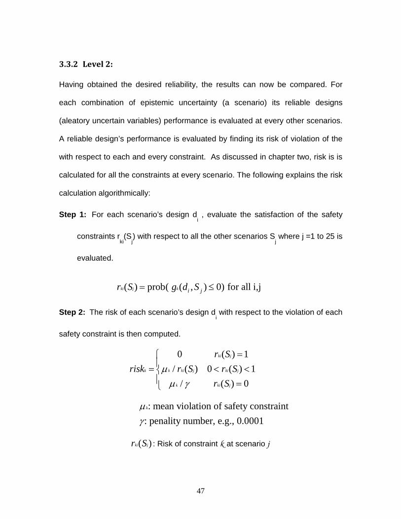
3.3.2 Level 2:
Having obtained the desired reliability, the results can now be compared. For
each combination of epistemic uncertainty (a scenario) its reliable designs
(aleatory uncertain variables) performance is evaluated at every other scenarios.
A reliable design’s performance is evaluated by finding its risk of violation of the
with respect to each and every constraint. As discussed in chapter two, risk is is
calculated for all the constraints at every scenario. The following explains the risk
calculation algorithmically:
Step 1: For each scenario’s design di , evaluate the satisfaction of the safety
constraints rki(S
j) with respect to all the other scenarios S
j where j =1 to 25 is
evaluated.
Step 2: The risk of each scenario’s design di with respect to the violation of each
safety constraint is then computed.
( )ki jr S : Risk of constraint k at scenario j
0 ( ) 1
/ ( ) 0 ( ) 1
/ ( ) 0
ki j
k k ki j ki j
k ki j
r S
risk r S r S
r S
µµ γ
=
= < < =
( ) prob( ( , ) 0) for all i,jki j k i jr S g d S= ≤
: mean violation of safety constraint
: penality number, e.g., 0.0001
kµγ

48
For this problem, there are ten constraints and twenty five scenarios, so
the risk vector has 250 entries. If there exists a single risk vector that has the
minimum risk value in each of the entries when compared to the other 24 risk
vectors, then the design associated with this risk vector is preferred over all the
other designs. If there is no such vector, which has the minimum risk for all the
constraints when compared to the other 25, an ideal risk vector whose entries
are all zeros is considered to proceed further. In other words in the ideal risk
vector the value of risk of all the constraints is zero. In this case, risk vector which
is most adjacent to zero risk vector is chosen as the least risky design. The
proximity of the vectors is computed using l 2 –norm.
Step3 : The design which has least risk is selected.
3.4 Results:
The following table shows the results of risk values as well as optimized weight of
the vehicle at the considered scenarios.
Scenario X10 X11
Car Wight after
optimization Risk
Scenario 1 -30.00 -30.00 29.69 116.78
Scenario 2 -30.00 -15.00 25.7 114.42
Scenario 3 -30.00 0.00 24.34 79.19
Scenario 4 -30.00 15.00 25.7 114.46
Scenario 5 -30.00 30.00 29.69 117.2
Scenario 6 -15.00 -30.00 28.05 97.69
Scenario 7 -15.00 -15.00 24.22 26.62
Scenario 8 -15.00 0.00 23.68 26
Scenario 9 -15.00 15.00 24.22 19.74
Scenario 10 -15.00 30.00 27.99 98.05
Scenario 11 0.00 -30.00 26.54 26.08
Scenario 12 0.00 -15.00 24.45 7.19

49
Scenario 13 0.00 0.00 24.12 42.71
Scenario 14 0.00 15.00 24.31 19.25
Scenario 15 0.00 30.00 26.54 26.31
Scenario 16 15.00 -30.00 25.08 8.98
Scenario 17 15.00 -15.00 24.99 3.66
Scenario 18 15.00 0.00 24.76 4.66
Scenario 19 15.00 15.00 24.35 15.98
Scenario 20 15.00 30.00 24.62 16.91
Scenario 21 30.00 -30.00 25.43 8.02
Scenario 22 30.00 -15.00 25.6 5.34
Scenario 23 30.00 0.00 25.42 6.2
Scenario 24 30.00 15.00 24.92 8.61
Scenario 25 30.00 30.00 24.45 17.77
Table 3-4: Results
In this problem the 17th scenario’s design performs well over all the
scenarios and has the least risk when compared to the designs of the remaining
scenarios. This is the preferred design.
This procedure, while allowing the practitioner to consider both aleatory and
epistemic uncertainties, and the associated risk of each solution over all the
scenarios, is computationally expensive. Typically, the number of epistemic
uncertain variables should be small, but one can see the significant
computational cost if these epistemic variables are discretized in smaller intervals
to obtain a better solution, and if the number of such variables increases.
Therefore, is there a more efficient way to identify the least risky solution? The
next chapter focuses on this aspect.

50
4 RISK SURFACE APPROXIMATION
Approximations may be used when sufficient resources are not available to
get exact responses out of the variables. Many real world engineering problems
are too complex to solve with many design variables to optimize. Sometimes
some of the problems may even be impossible to solve using the available
analytical tools. Even when the exact representation can be obtained,
approximation may be used to attain reasonably accurate responses while
reducing the computation time significantly. In our case, approximations are
employed to decrease the computational cost. Discretization of the epistemic
variables in the methodology presented earlier is arbitrary. The finer the
discretization is, the higher is the precision of the result. However the
computational cost also increases with discretization. To begin with, each
epistemic variable is divided into five discrete steps and the data obtained is
used to approximate the responses. Thus how can one approximate the data
over the whole range independently on the granularity of the discretization?
Commonly, responses are approximated at three levels namely local, mid range
and global [53].
4.1 Local Approximations:
At the local level, responses are approximated in the neighborhood of
design. Three popular local approximation techniques are the Linear Taylor
series, the Reciprocal, and the Conservative or Hybrid.

51
4.1.1 Linear Taylor Series Approximation:
A Linear Taylor approximation [54] is an approximation of responses using
a first order Taylor’s expansion, which uses terms of degree less than or equal to
one from the original Taylor series. Though Linear Taylor Series approximations
are widely used methods, they need move limits since they are only valid in the
close neighborhood of a point unless the functions are linear [53].
Original Taylor Series:
or
( ) ( ) ( ) ( ) ( ) ( ) ( ) ( )( )
2''' ...... ....
2! !
nnf a f a
f x f a f a x a x a x an
= + − + − + + − +
First order Taylor Series:
If f(x) is a function and a is a point, then the function f(x) about a point a
( ) ( ) ( )( )'f x f a f a x a≅ + −
00 0
( )( ) ( ) ( )i
i i
f xf x f x x x
x
∂= + −
∂∑
52
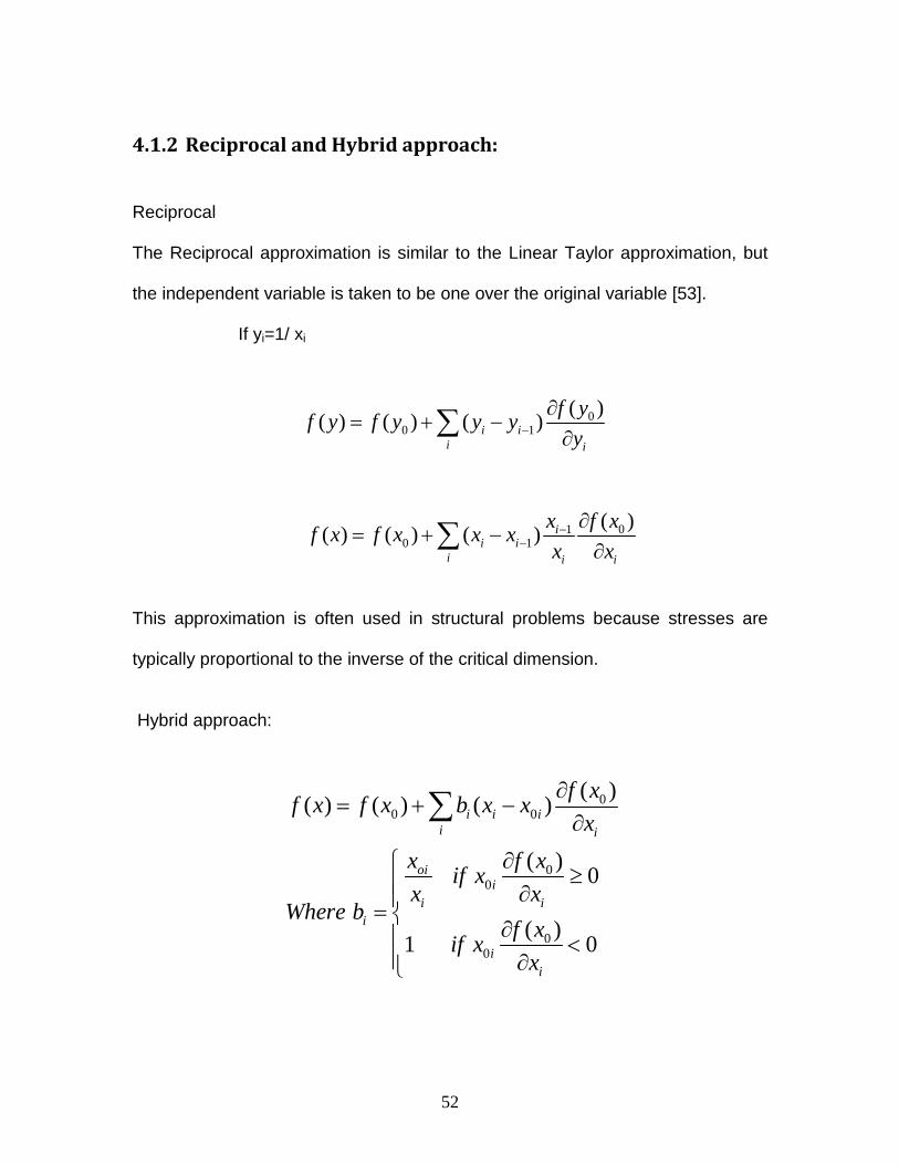
4.1.2 Reciprocal and Hybrid approach:
Reciprocal
The Reciprocal approximation is similar to the Linear Taylor approximation, but
the independent variable is taken to be one over the original variable [53].
If yi=1/ xi
This approximation is often used in structural problems because stresses are
typically proportional to the inverse of the critical dimension.
Hybrid approach:
00 1
( )( ) ( ) ( )i i
i i
f yf y f y y y
y−
∂= + −
∂∑
1 00 1
( )( ) ( ) ( ) i
i ii i i
x f xf x f x x x
x x−
−
∂= + −
∂∑
00 0
00
00
( )( ) ( ) ( )
( )0
( )1 0
i i ii i
oii
i ii
ii
f xf x f x b x x
x
x f xif x
x xWhere b
f xif x
x
∂= + −
∂
∂ ≥ ∂=
∂ < ∂
∑

53
The hybrid approach combines both the linear and reciprocal approximations,
and has therefore a slightly larger domain of application. It is however still a local
approximation which depends on move limits to prevent the algorithm from using
approximations that are too far off from the results of the original functions [53].
4.2 Mid-range Approximations:
The information obtained from previous points can be used to improve the
approximation and is used for Mid-range approximations. In 1990, Dr.Fadel [55]
in his “Two Point Exponential Approximation Method for Structural Optimization”
introduced a two point exponential approximation method in extension to the
Taylor series to design a mid range approximation.
These approximations as well as the local approximations are not
appropriate to be used as surrogates for exact models that are valid over a large
area of the design space. Local approximations are only valid in the immediate
vicinity of a current point, mid range approximation extend that range, but are still
around the specific point, only global approximations are valid over a large
domain in the design space.
4.3 Global Approximations:
Responses which are approximated at the global level are called global
approximations. Three famous global approximation methods are Response
surface, Kriging, and Neural Networks [53].

54
4.3.1 Response surface Methodology:
The Response Surface Methodology (RSM) was first introduced by George
E. P. Box And K. B. Wilson in 1951[56]. In 2003, Myers [57] wrote “Response
surface methodology (RSM) is a collection of mathematical and
statistical methods that are used to develop, to improve, or to optimize a product
or process”. Montgomery [58], writes that “As an important subject in the
statistical design of experiments, the Response Surface Methodology (RSM) is a
collection of mathematical and statistical techniques useful for the modeling and
analysis of problems in which a response of interest is influenced by several
variables and the objective is to optimize this response”. However, typically the
RSM is a second order approximation, through which a global response is
obtained over the design space. In order to get a better response surface, the
sample input points must be selected carefully. The Design of Experiment is an
efficient way to generate such sample points. Random methods, diagonal design,
full grid, central composite, Box-Behnken Designs, Factorial Designs, Latin
Hypercube, Orthogonal Arrays are some of the some of the design of experiment
techniques commonly described in the literature for such a purpose.
Refer to “Response surface methodology 1966-1988” by Myers et al [59] to
know more about the development of RSM.
4.3.1.1 Advantages of RSM:
• It may be useful when a small amount of empirical data is available.

55
• It may be useful to obtain significant features in the data.
• It may be useful to recognize the regions of interest in the design space.
• It may help in understanding the problem under study in detail.
• It may help in moving faster towards the optimum.
4.3.1.2 Disadvantages of RSM
• Inaccuracy of the data may be misleading.
• Responses of highly nonlinear models may not be accurate enough.
Considering the nonlinearity of the problem, diversity in the bounds of design
variables and the desirable level of accuracy, it is presumed that a response
surface which can also capture the deviation would be better for the problem.
Hence, Kriging was chosen to generate the approximations.
4.3.2 Kriging:
Kriging is an interpolation technique, developed by D. G. Krige [60] a
South African Engineer in 1950s to determine ore grades. He and G. Matheron, a
French mathematician, improved it further. It is a combination of response
surface and the deviations from that surfaces. It is one of the more popular
approximation techniques used for deterministic empirical data [61]. It is also
called DACE, which stands for Design and Analysis of Computer Experiments
[53]. The application areas of kriging include Structural Optimization,
Multidisciplinary Design Optimization, Geostatistics, Mechanical Engineering, etc
[62-64].

56
4.3.2.1 Advantages of Kriging:
• The Kriging method is flexible to approximate wide variety of complex and
non-linear models.
• Better accuracy may be obtained using Kriging techniques.
4.3.2.2 Drawbacks of Kriging:
• Computationally expensive when compared to other approximation
methods [61].
Since Kriging is capable of capturing the deviations, and is flexible enough to
approximate highly nonlinear problems accurately, it is chosen over the other
approximation techniques.
4.4 Approach
An approximation toolbox, Design and Analysis of Computer Experiments
(DACE) [65], is used to generate the responses. DACE is a Matlab toolbox. It
uses kriging approximations to generate responses. The developers write that
“Typical use of this software is to construct a kriging approximation model based
on data from a computer experiment and to use this approximation model as a
surrogate for the computer model” [65].
This toolbox is selected to generate risk surfaces because of its accuracy in
generating the surfaces. Fifteen different polynomial functions are considered for
the study to test the accuracy of the toolbox. Out of which five are listed in table
57
4-1(The rest can be found in appendices). Twenty five sample points are
generated using a Latin hypercube sampling [47] to generate the response
surface using DACE.
4.5 Testing the accuracy of the toolbox
The accuracy of the approximated surface is tested by finding the value of
the function under study at the points which were not used to generate the
approximation and comparing these values with the original function values at
the same points. Say x, y are control variables and “r” is response variable.
( , )r f x y=
For computer models, often the relation between r, x, y is unknown. But here to
test the accuracy of the toolbox, functions whose relation between the control
variables and response variables is known are considered (see table 5). 25 set of
points are generated for the control variables within the assumed limits using
Latin hypercube sampling and their responses are calculated using the actual
functional relation between the control variables and response variables. This
data is given as input to the toolbox and the approximated surfaces are
generated.
Example:

58
[ ][ ]
1,10
20,30
x
y
r x y
∈
∈
= +
For x=1, 5, 10 and y = 20, 25, 30 then r = 21, 30, 40. Using this data as input for
the tool box the corresponding approximate response is generated. The value of
the original function at an untried point (which is not given as input to the toolbox)
x=2, y= 25, is r = 27. If the value obtained by the approximated surface is 29,
then the error is:
29 27100
27error
− = ×
= 7.4 In summary, the percentage error is calculated as:
( )100
Estimated Value Original Valueerror
Original Value
−= ×
The tool box approximation is tested on several test function to study its
accuracy. The following equations and bounds (table 5) are used to perform
these tests.

59
S.No Equation Variable bounds
1. r = 100*(y-x.^2).^2 + (1-x).^2; [63] x є [-5,5], y є [-5,5]
2. r=x.^2-y.^2+x.*y + x-y; x є [-5,5], y є [-5,5]
3. r=x.^4 - y.^4; x є [-5,5], y є [-5,5]
4. r=exp(x) + exp(y); x є [-5,5], y є [-5,5]
5. r=sin(x)^2 + sin(y)^2; x є [-5,5], y є [-5,5]
Table 4-1: Equations used to test the toolbox

60
The results obtained are illustrated graphically below.
4.5.1 Function 1: Rosenbrock function
Figure 4-1: Original Rosenbrock Function
Figure 4-2: DACE approximation

61
Error Calculation:
Untried coordinates: (4,4)
Actual function value is 14409
Approximated surface value is 15445
Percentage error is : 7.18
4.5.2 Function 2
Figure 4-3: Actual function

62
Figure 4-4: DACE approximation
Error Calculation:
Untried coordinated (4,4)
Actual function value is 16
Approximated surface value is 16.16
Percentage error is : 1

63
4.5.3 Function 3
Figure 4-5: Actual Function
Figure 4-6: DACE Approximation
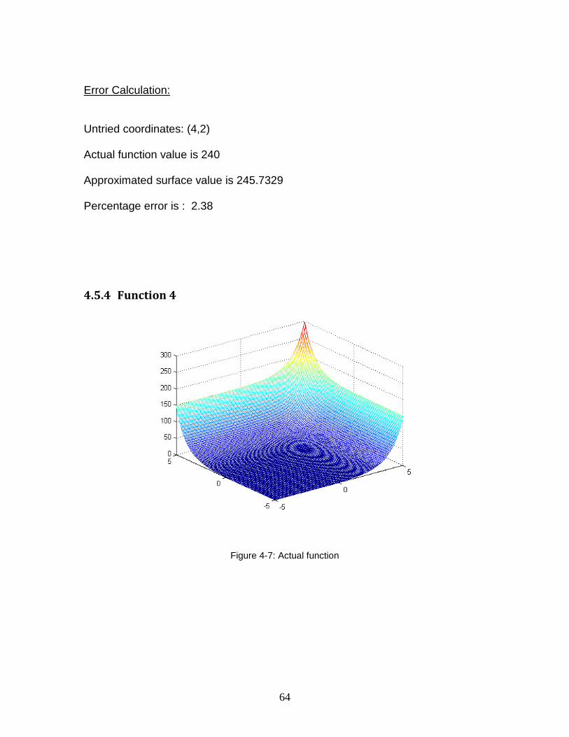
64
Error Calculation:
Untried coordinates: (4,2)
Actual function value is 240
Approximated surface value is 245.7329
Percentage error is : 2.38
4.5.4 Function 4
Figure 4-7: Actual function

65
Figure 4-8: DACE Approximation
Error Calculation:
Untried coordinates: (4,2)
Actual function value is 47.2095
Approximated surface value is 47.9
Percentage error is : 1.46

66
4.5.5 Function 5
Figure 4-9: Actual function
Figure 4-10: DACE Approximation

67
Error Calculation:
Untried coordinates: (4,2)
Actual function value is 1.3995
Approximated surface value is 1.2807
Percentage error is: 8.49
As mentioned earlier, the accuracy of these response surfaces was tested
by comparing the function values of original function and DACE functions at
untried data points. Except for exceptionally nonlinear functions like the fifth
function the toolbox worked well for the rest of the functions. Hence, this toolbox
was used to generate the risk surfaces which are discussed in detail in the
following section.
4.6 Risk surfaces:
Risk surfaces are generated with the variables X10 (barrier hitting height)
and X11 (barrier hitting position) on X and Y axes and risk value on the Z axis.
Though risk is a function of variables from X1 to X11.The reasons behind choosing
X10 and X11 alone to generate surface is:
• Finding the least risky combination of epistemic variables (scenario) is of
interest.
• X1 to X7 are distributed within a range.

68
• X10 and X11 are independent and they are not affected by any other design
variables nor have any relation with other variables.
Fitting the response surface as a function of the epistemic variables has not been
done in the past, and seems counterintuitive since the risk is evaluated at all the
scenarios and over the range of aleatory variables. Yet the former method
arbitrarily discretizes the epistemic variables, and the solution chosen is the one
that has the lowest risk over all the scenarios. That risk is evaluated for the
solution at each scenario, and implicitly, the risk is therefore a function of the
epistemic variables. This hypothesis has to be further validated, but it will be
explored in this work on the specific example described earlier.
In order to test the consistency of the risk surface, each epistemic variable is
divided into several discrete steps. The discretization is purely arbitrary and the
numbers of scenarios considered are 9, 16, 25, 49, and 169. The below shown
are the approximated risk surface for the respective number of scenarios.

69
4.6.1 Using 9 scenarios
Figure 4-11: Risk Surface Approximation for 9 scenarios

70
4.6.2 Using 16 scenarios
Figure 4-12: Risk Surface Approximation for 16 scenarios
4.6.3 Using 25 scenarios
Figure 4-13: Risk Surface Approximation for 25 scenarios

71
4.6.4 Using 49 scenarios:
Figure 4-14: Risk Surface Approximation for 49 scenarios
4.6.5 Using 169 scenarios:
Figure 4-15: Risk Surface Approximation for 169 scenarios
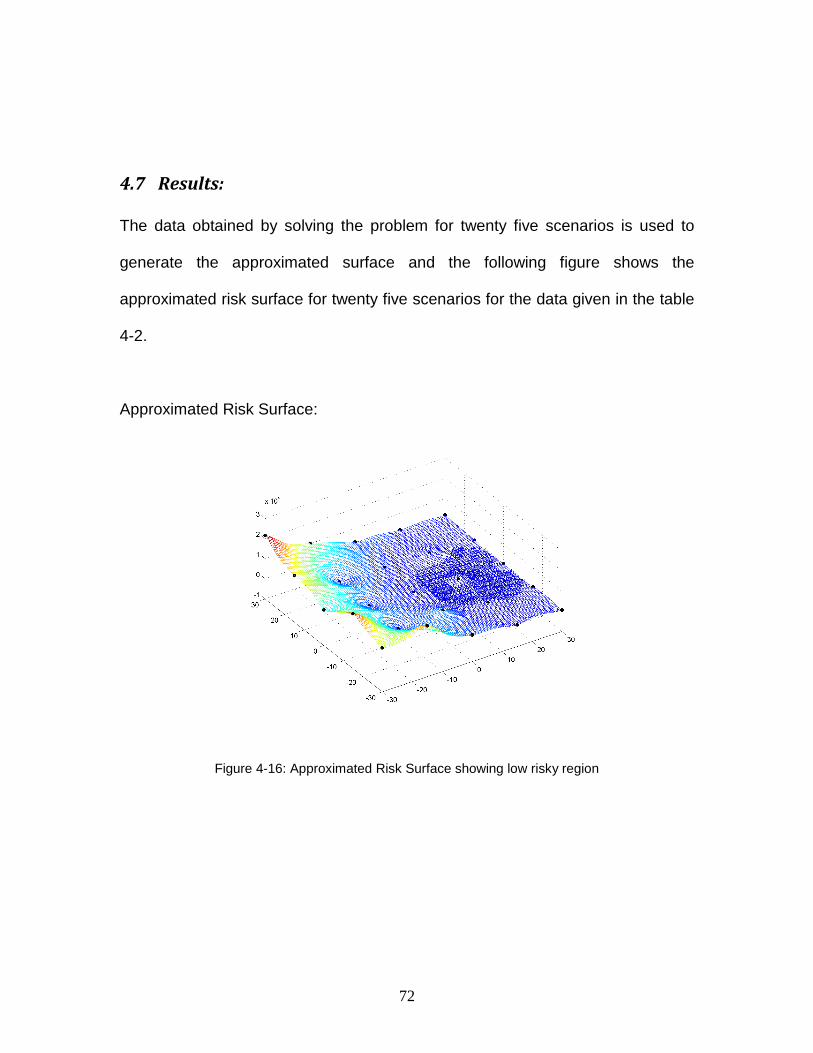
72
4.7 Results:
The data obtained by solving the problem for twenty five scenarios is used to
generate the approximated surface and the following figure shows the
approximated risk surface for twenty five scenarios for the data given in the table
4-2.
Approximated Risk Surface:
Figure 4-16: Approximated Risk Surface showing low risky region

73
Figure 4-17: Approximated Risk Surface showing low risky region

74
Scenario X10 X11
Car Weight after
optimization Risk
Scenario 1 -30.00 -30.00 29.69 116.78
Scenario 2 -30.00 -15.00 25.7 114.42
Scenario 3 -30.00 0.00 24.34 79.19
Scenario 4 -30.00 15.00 25.7 114.46
Scenario 5 -30.00 30.00 29.69 117.2
Scenario 6 -15.00 -30.00 28.05 97.69
Scenario 7 -15.00 -15.00 24.22 26.62
Scenario 8 -15.00 0.00 23.68 26
Scenario 9 -15.00 15.00 24.22 19.74
Scenario 10 -15.00 30.00 27.99 98.05
Scenario 11 0.00 -30.00 26.54 26.08
Scenario 12 0.00 -15.00 24.45 7.19
Scenario 13 0.00 0.00 24.12 42.71
Scenario 14 0.00 15.00 24.31 19.25
Scenario 15 0.00 30.00 26.54 26.31
Scenario 16 15.00 -30.00 25.08 8.98
Scenario 17 15.00 -15.00 24.99 3.66
Scenario 18 15.00 0.00 24.76 4.66
Scenario 19 15.00 15.00 24.35 15.98
Scenario 20 15.00 30.00 24.62 16.91
Scenario 21 30.00 -30.00 25.43 8.02
Scenario 22 30.00 -15.00 25.6 5.34
Scenario 23 30.00 0.00 25.42 6.2
Scenario 24 30.00 15.00 24.92 8.61
Scenario 25 30.00 30.00 24.45 17.77
Table 4-2: Input data to generate risk surface
According to the risk formula given in chapter two, risk cannot go below zero.
Since this is an approximated surface, all the risk values which are below zero
are treated as zero risk values. The dark blue region represents the scenarios
which have a risk of zero or below zero. For the above computed surface

75
approximation, NLPQ algorithm is used to find the minimum. The obtained
minimum is at the scenario (20.81, -2.83). Usually it takes two minutes to
calculate a reliable design for one scenario for a laptop with a core2duo
processor T8100 @2.10GHz and 4.00GB RAM. If there are 50 scenarios the
computation time would be 100 minutes. But by using these approximation
techniques the computation time can be reduced significantly. The table 4-3 and
4-4 shown below justifies the use of approximations and the reduction in
computational time.
Before approximation:
Number of scenarios
given as input Best Scenario Weight of the car Computational time
in minutes 25 X
10=15; X
11=-15 24.69 48.89
49 X10
=10; X11
=-10 24.497 100.81
169 X10
=20; X11
=0 24.49 237.24
Table 4-3: Results Before approximation
After approximation:
Best Scenario Weight of the car Computational time
in minutes Minimum found
without
Approximation X
10=15; X
11=-15 24.49 237.24
Minimum after
Approximation X
10=20.81; X
11=-2.83 24.62 52
Table 4-4: Results after approximation

76
4.8 Exploring the hypothesis of risk surfaces:
Originally, the δ chosen by the authors for this problem is 30mm. As
explained earlier, if the selected impact point is at coordinates (0, 0), the hitting
height and hitting position can be within a range of -δ to δ from the impact point.
Hence, earlier the barrier hitting point can be anywhere above or below the
selected impact point within a 30mm range. But by restricting the movability of
the barrier by confining the hitting region to single direction (horizontal or vertical)
the hypothesis is explored further.
Case 1
Assume x11 as 0. Hence, the movability of barrier is restricted in horizontal
direction i.e., the barrier can only move in vertical direction. x10 ranging from -30
to 30 and x11 being 0, we discretize the epistemic variable x10 and apply the
approach.
Figure 4-18: x10 є [-30,30] & x11=0

77
Before approximation the minimum risk is at scenario x10=15 and x11=0 from
among the scenarios, and after approximating and the curve and optimizing
(using NLPQ) it the risk at x10=19.28 and x11=0.
Case 2:
Considering x11 as 30 and x10 ranging from -30 to 30; before approximation the
minimum risk is at scenario (0, -30) and after approximating the curve and finding
the minimum using NLPQ the minimum is at (-4,-30).
Figure 4-19: x10 є [-30, 30] & x11=-30 Case 3: Confining x11 to -30 and x10 ranging from -30 to 30; before approximation the
minimum risk is at scenario (15, 30) and after approximating the curve and
finding the minimum using NLPQ the minimum is at (22,30).

78
Figure 4-20: x10 є [-30, 30] & x11= 30
Since, there is not much variation in the risk values of scenarios in the risk
surfaces (presented in the previous section) and risk values of scenarios in risk
curves presented in this section and also there is not much difference in the
coordinates of scenarios values which have minimum risk, the credibility of the
risk surface as a function of epistemic uncertain variables is valid for this
problem.
79
5 CONCLUSION AND FUTURE WORK
The main idea behind the research work presented in the thesis is to provide
a step wise procedure that aids engineers as well as decision makers to make
decisions under uncertainty. Many methods in the literature have been dealing
with uncertainties but very few of them consider after effects of violation of a
design and the risk associated with such a decision as an additional criterion in
design selection. The method proposed by researchers at Clemson University
discussed in the thesis not only considers reliability percentage of a design but
also considers after effects of its violation during the design selection process.
To begin with, for a desired reliability percentage, the problem is solved for
few scenarios (combination of epistemic variables) and a reliable design is
computed at each scenario. For every scenario’s reliable design, the chances of
violation of that design with respect to all the constraints at other scenarios are
computed. The after affects of violation are also considered during the
calculation of these chances. The scenario and its respective reliable design
which has least chances of violation are preferred in deciding a solution.
However, the more the epistemic variables are, and the finer the discretization of
these epistemic variables, the more the problem becomes computationally
expensive in this approach because, the problem has to be solved at each
combination of these discretized variables. The computational burden could be

80
reduced by selecting few scenarios, which capture the behavior of risk as a
function of epistemic variables, in order to estimate the problem behavior and
interpolating the behavior at the rest of the scenarios. For this purpose surface
approximation techniques are employed in this thesis.
Before selecting an approximation technique, many methods were tested
for their accuracy using different functions. However, depending on the nature
and environment of the problem, the second order Kriging method is selected to
approximate the risk. To implement the Kriging approximation technique a
toolbox named DACE is chosen after testing its accuracy using twenty five
different functions.
The main idea is to identify the scenarios which have low risk values and
find the best among them. Hence a plausible attempt is made by approximating
the risk values only as a function of epistemic uncertain variables. This attempt
is subjective because of the nature of the problem.
In summary, the first chapter discusses how uncertainty is defined in
different fields and how is it distinct in the field of engineering. It explains how to
recognize the sources of uncertainty how uncertainties are classified in literature.
It also explains the uncertainty modeling techniques present in the literature and
how they model the uncertainties. Then expands on how is risk different from
uncertainty in engineering design. Chapter one concludes by presenting the
motivation behind this research. Chapter two elucidates the methodology that is
proposed by researchers at Clemson University. In chapter three, an application

81
problem is presented to explain and test the methodology. Chapter four explains
the technique which is employed and explored to make the methodology
(proposed in chapter two) more computationally efficient.
An approximated surface, as a function of the epistemic variables is
generated, which has not yet been attempted in the literature. The validity of the
technique, for this particular problem, is tested by approximating risk surfaces
using various numbers of scenarios. Since the risk is evaluated for the solution at
each scenario, and implicitly the risk is a function of the epistemic variables. This
hypothesis has to be further validated, but it is explored in this work on the
specific example described in chapter three.
However, advantages are obtained at some cost; there is a scope for
improvement for this work in the following areas: step size selection and scenario
selection. There may be a better way in selecting the step size during the
process of tightening a constraint. Rather than selecting choosing the scenarios
in an arbitrary way if there can be a way to choose scenarios that captures most
of the critical points of the risk surface computational burden can be reduced
even more.
The main take away from this work are a stepwise procedure that helps in
handling uncertainty in a systematic way, handling computationally expensive
problems involved more number of epistemic uncertainties.

82
APPENDICES
The following are the other functions that are used to test the tool box:
S.No Equations Variable
bounds
Untried
point
Original
value
Dace
value
Percentage
error
1. r = x3+y
3+x
2+y
2+x+y x є [-5,5], y є [-5,5] (4,5) 239 232.2921 2.81
2. r= x3+y
3+x
2y
2 x є [-5,5], y є [-5,5] (4,5) 589 588.0559 0.1%
3. Easom’s function x є [-5,5], y є [-5,5] (4,4) -0.0979 -0.0817 16.49%
4. Michalewicz’s
function
x ,y є [1.5,2.5] (2,2) -0.3702 -0.3942 6.51%
5. Goldstein price
function
x, y є [-3,3] (0,-1) 3 3.4680 15.6%
6. r= xy- x
2y
2
x, y є [-3,3] (2,2) 12 -13.5376 12.81%
7. r = x
2+y
2
x, y є [-3,3] (2,2) 32 32 0%
8. r=2sin(x)+5sin(y)
x, y є [-3,3] (2,2) 6.3651 6.3651 0%
9. r = x
3y+ xy
3
x, y є [-3,3] (2,2) 32 31.15 2.64%
10. r = x
3+y
2- xy
x, y є [-3,3] (2,2) 8 8.01 1.9%

83
Function1:
Figure 5-1: Before Approximation
Figure 5-2: After approximation

84
Function 2:
Figure 5-3: Original Function
Figure 5-4: After approximation

85
Function 3:
Figure 5-5: Original function
Figure 5-6: After approximation

86
Function 4:
Figure 5-7: Original function
Figure 5-8: After Approximation

87
Function 5:
Figure 5-9: Original function
Figure 5-10: After approximation

88
Function 6:
Figure 5-11: Original Figure
Figure 5-12: After Approximation

89
Function 7:
Figure 5-13: Original function
Figure 5-14: After approximation
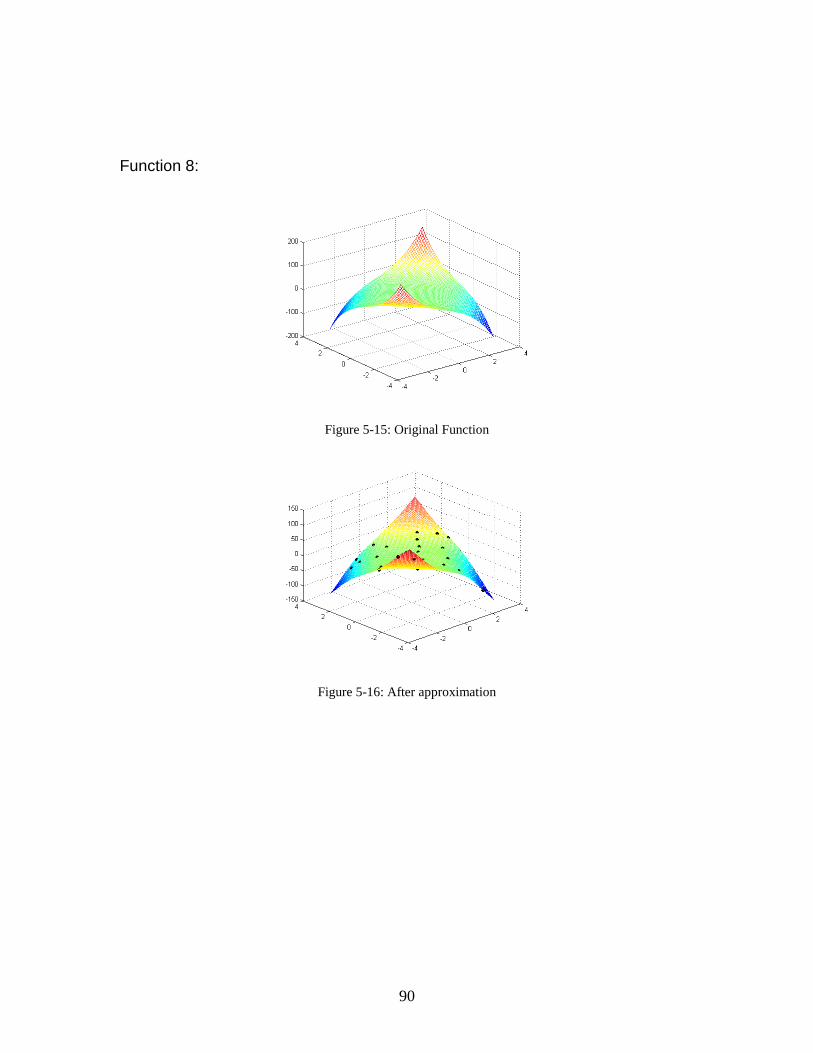
90
Function 8:
Figure 5-15: Original Function
Figure 5-16: After approximation

91
Function 9:
Figure 5-17: Original Function
Figure 5-18: After approximation

92
Function 10:
Figure 5-19: Original function
Figure 5-20: After approximation

93
REFERENCES
[1]http://wordnetweb.princeton.edu/perl/webwn?s=Uncertainty&o2=&o0=1&o7=&
o5=&o1=1&o6=&o4=&o3=&h=.
[2] http://www.merriam-webster.com/dictionary/uncertainty
[3] http://www.epa.gov/riskassessment/glossary.htm#u.
[4] F. H. Knight. Risk, uncertainty and profit.pages381,Boston, New York 1921.
[5] L. G. Epstein. A definition of uncertainty aversion. The Review of Economic
Studies, 66(3):579-608, 1999.
[6] G. J. Klir and M. J. Wierman. Uncertainty-based information : elements of
generalized information theory.pages168,Physica-Verlag 1999.
[7] http://www.informit.com/articles/article.aspx?p=21313.
[8] E. Hund, D. L. Massart and J. Smeyers-Verbeke. Operational definitions of
uncertainty. TrAC Trends in Analytical Chemistry, 20(8):394-406, 2001.
[9] J. L. Dungan, D. Gao and A. T. Pang. Definitions of Uncertainty. 2002.
[10] Moss, R.H. and Schneider, S.H.,. Uncertainties in the IPCC TAR:
Recommendations to lead authors for more consistent assessment and
reporting. World Meteorological Organization, 33-51, Geneva, 2000.
[11] A. H. Willet. The economic theory of risk and insurance.pages142, 1901.
[12] J. M. Keynes. The general theory of employment, interest and
money.pages403,New York 1935.

94
[13] K. A. Der. Measures of structural safety under imperfect states of
knowledge. Journal of Structural Engineering New York, N.Y., 115(5):1119-1140,
1989.
[14] G. W. Parry. The characterization of uncertainty in probabilistic risk
assessments of complex systems. Reliab.Eng.Syst.Saf., 54(2-3):119-126, 1996.
[15] W. L. Oberkampf, J. C. Helton, C. A. Joslyn, S. F. Wojtkiewicz and S.
Ferson. Challenge problems: Uncertainty in system response given uncertain
parameters. Reliab.Eng.Syst.Saf., 85(1-3):11-19, UK, 2004.
[16] J. C. Helton. Treatment of uncertainty in performance assessments for
complex systems. Risk Analysis, 14(4):483-483, New York, NY, USA, 1994.
[17] http://dictionary.reference.com/browse/aleatory.
[18] http://www.merriam-webster.com/dictionary/epistemic.
[19] National Research Council(U.S) and Committee on Risk-Based Analysis for
Flood Damage Reduction. Risk analysis and uncertainty in flood damage
reduction studies.pages216, 2000.
[20] http://www.ce.memphis.edu/7137/PDFs/Abrahamson/C05.pdf.
[21] T. O'Hagan. Dicing with the unknown. Significance, 1(3):132-133, 2004.
[22] L. P. Swiler, T. L. Paez and R. L. Mayes. Epistemic Uncertainty
Quantification Tutorial. In proc. of Proceedings of the IMAC-XXVII, 2009.
[23] H. Agarwal and J. E. Renaud. Reliability based design optimization using
response surfaces in application to multidisciplinary systems. Engineering
Optimization, 36(3):291-311, 2004.

95
[24] L. A. Zadeh. Fuzzy sets. Information and Control, 8(3):338-353, 1965.
[25] L. A. Zadeh. Fuzzy sets as a basis for a theory of possibility. Fuzzy Sets
Syst., 1(1):3-28, 1978.
[26] L. A. Zadeh. Fuzzy sets as a basis for a theory of possibility. Fuzzy Sets
Syst., 100(Supplement 1):9-34, 1999.
[27] J. Aughenbaugh Matthew. Managing uncertainty in engineering design
using imprecise probabilities and principles of information economics.United
States -- Georgia 2006.
[28] D. Didier and P. Henri.Possibility theory: An approach to computerized
processing of uncertainty. International Journal of General Systems, 15(2):263
pages, 1989.
[29] G. Shafer. A mathematical theory of evidence.pages302, 1976.
[30] http://www.merriam-webster.com/dictionary/probability.
[31] A. Kolmogorov. Foundations of the theory of probability. 1956.
[32] Z. P. Mourelatos and J. Zhou. A design optimization method using
evidence theory. Transactions of the ASME.Journal of Mechanical Design,
128(4):901-8, USA, 2006.
[33]http://www.solver.com/riskanalysis/tutorial.htm#How_are_Uncertainty_and_R
isk_Different.

96
[34] S. Samson, J. A. Reneke and M. M. Wiecek. A review of different
perspectives on uncertainty and risk and an alternative modeling paradigm.
Reliability Engineering and System Safety, 94(2):558-567, Langford Lane,
Kidlington, Oxford, OX5 1GB, United Kingdom, 2009.
[35] R. I. Mehr and E. Cammack. Principles of Insurance.pages904, 1961.
[36] J. H. Magee. General insurance.pages913, 1947.
[37] J. Philippe. Value at risk: the new benchmark for managing financial
risk.pages602, 2001.
[38] R. T. Rockafellar. Coherent Approaches to Risk in Optimization Under
Uncertainty.pages38-61,INFORMS 2007 2007.
[39] http://mathworld.wolfram.com/L2-Norm.html.
[40] A. H. Roger and R. J. Charles. Matrix analysis.pages561, 1990.
[41] D. B. Bois, C. C. Chou, B. B. Fileta, T. B. Khalil, A. I. King, H. F. Mahmood,
J. Wismans and H. J. Mertz. Vehicle Crashworthiness and Occupant
Safety.pages388, 2004.
[42] Ren-Jye Yang, A. Akkerman, D. F. Anderson, O. M. Faruque and Lei Gu.
Robustness optimization for vehicular crash simulations. Computing in Science &
Engineering, 2(6):8-13, 2000.
[43] L. Gu, R. J. Yang, C. H. Tho, M. Makowski, O. Faruque and Y. Li.
Optimization and robustness for crashworthiness of side impact. Int.J.Veh.Des.,
26(4):348-60, Switzerland, 2001.

97
[44] K. Sinha. Reliability-based multiobjective optimization for automotive
crashworthiness and occupant safety. Structural and Multidisciplinary
Optimization, 33(3):255-268, Tiergartenstrasse 17, Heidelberg, D-69121,
Germany, 2007.
[45] http://www.euroncap.com/home.aspx.
[46] http://autorepair.about.com/library/faqs/bl996g.htm.
[47] M. D. McKay, R. J. Beckman and W. J. Conover. A Comparison of Three
Methods for Selecting Values of Input Variables in the Analysis of Output from a
Computer Code. In proc. of Technometrics, pages239-245, 1979.
[48] B. D. Youn and K. K. Choi. A new response surface methodology for
reliability-based design optimization. Comput.Struct., 82(2-3):241-56, UK, 2004.
[49] B. D. Youn, K. K. Choi, R. -. Yang and L. Gu. Reliability-based design
optimization for crashworthiness of vehicle side impact. In proc. of Structural and
Multidisciplinary Optimization, pages272-83, 2004.
[50] http://eevc.org/.
[51] R. H. Myers, D. Montgomery C. and C. Anderson-Cook M. Response
Surface Methodology: Process and Product Optimization Using Designed
Experiments.pages704, 2009.
[52] http://www.merriam-webster.com/dictionary/reliability.
[53] G. M. Fadel. ME 871 Lecture notes. 2008.
[54] http://www.math.unh.edu/~jjp/taylor/taylor.html.

98
[55] G. M. Fadel. Two point exponential approximation method for structural
optimization. Struct.Opt., 2(2):117-124, 1990.
[56] G. E. P. Box and K. B. Wilson. On the experimental attainment of optimum
conditions. Journal of the Royal Statistical Society.Series B (Methodological),
13(1):1-45, 1951.
[57] W. R. Myers. Response surface methodology. Encyclopedia of
Biopharmaceutical Statistics: Second Edition, 2003.
[58] D. C. Montgomery. Design and analysis of experiments.New York [etc.]
1991.
[59] R. H. Myers. Response surface methodology: 1966-1988. Technometrics,
31(2):137, 1989.
[60] D. G. Krige. A statistical approach to some basic mine evaluation problems
on the witwatersrand. Computing, 99, 2000.
[61] J. D. Martin. Use of kriging models to approximate deterministic computer
models. AIAA J., 43(4):853, 2005.
[62] T. W. Simpson. Approximation methods in multidisciplinary analysis and
optimization: A panel discussion. Structural and Multidisciplinary Optimization,
27(5):302, 2004.
[63] T. W. Simpson. Kriging models for global approximation in simulation-
based multidisciplinary design optimization. AIAA J., 39(12):2233, 2001.

99
[64] A. Chiralaksanakul and S. Mahadevan. First-order approximation methods
in reliability-based design optimization. Transactions of the ASME.Journal of
Mechanical Design, 127(5):851-7, USA, 2005.
[65] http://www2.imm.dtu.dk/~hbn/dace/.