Design of a cargo load carrying structure for a hybrid air vehicle

Lena Olsson

lenols@kth.se

Master of Science Thesis, September 2016 KTH Royal institute of Technology, Department of lightweight structures

SE-100-44 Stockholm

ii

Sammanfattning Framsteg inom flygindustrin har resulterat i hybridluftskepp, en kombination av aerostater och aerodyner med möjligheten att landa utan infrastruktur och med minimal markbemanning. Detta arbetet utforskar möjligheten att använda en mjuk typ av dessa farkoster för godstransport. För att göra det krävs en lastbärare som kan överföra lastens tyngd till givna fästpunkter på den mjuka och deformabla luftskeppskroppen. En kortare förstudie undersöker gränserna och rimligheten i olika lasttyper. Slutsatsen är att det finns tre typer av karaktäristiskt olika problem som kan kombineras för att representera de flesta realistiska lastfallen. Ett modulärt bärsystem konstrueras i form av olika moduler som representerar dessa problem. Lämpliga dimensioner bestäms sedan genom att ta fram sambanden för de spänningar och deformationer som uppstår vid förväntad belastning.

Abstract Recent developments in aeronautics have resulted in hybrid airships, a combination of aerostats and aerodynes with the ability to land without infrastructure and using minimal ground crew. This work explores the possibility of using a non rigid type of these vehicles for cargo transportation. To do so, a load carrier able to transfer the load to an allotted set of attachment points under the soft hull of the airship is needed. A short prestudy examines the limits and feasibilities of potential cargo-types and concludes there are three characteristically different problems that can be combined to represent most realistic load cases. A modular carrier system is then created with modules corresponding to each problem, and suitable dimensions are chosen by finding the relations to the resulting stresses and deflections.

iii

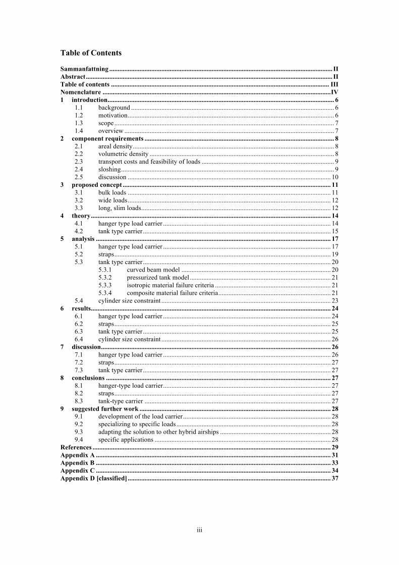
Table of Contents Sammanfattning ..................................................................................................................................... II Abstract ................................................................................................................................................... II Table of contents .................................................................................................................................. III Nomenclature ........................................................................................................................................ IV 1 introduction ....................................................................................................................................... 6 1.1 background ......................................................................................................................... 6 1.2 motivation ........................................................................................................................... 6 1.3 scope ................................................................................................................................... 7 1.4 overview ............................................................................................................................. 7 2 component requirements ................................................................................................................. 8 2.1 areal density ........................................................................................................................ 8 2.2 volumetric density .............................................................................................................. 8 2.3 transport costs and feasibility of loads ............................................................................... 9 2.4 sloshing ............................................................................................................................... 9 2.5 discussion ......................................................................................................................... 10 3 proposed concept ............................................................................................................................ 11 3.1 bulk loads ......................................................................................................................... 11 3.2 wide loads ......................................................................................................................... 12 3.3 long, slim loads ................................................................................................................. 12 4 theory ............................................................................................................................................... 14 4.1 hanger type load carrier .................................................................................................... 14 4.2 tank type carrier ................................................................................................................ 15 5 analysis ............................................................................................................................................ 17 5.1 hanger type load carrier .................................................................................................... 17 5.2 straps ................................................................................................................................. 19 5.3 tank type carrier ................................................................................................................ 20

5.3.1 curved beam model ......................................................................................... 20 5.3.2 pressurized tank model .................................................................................... 21 5.3.3 isotropic material failure criteria ..................................................................... 21 5.3.4 composite material failure criteria ................................................................... 21

5.4 cylinder size constraint ..................................................................................................... 23 6 results ............................................................................................................................................... 24 6.1 hanger type load carrier .................................................................................................... 24 6.2 straps ................................................................................................................................. 25 6.3 tank type carrier ................................................................................................................ 25 6.4 cylinder size constraint ..................................................................................................... 26 7 discussion ......................................................................................................................................... 26 7.1 hanger type load carrier .................................................................................................... 26 7.2 straps ................................................................................................................................. 27 7.3 tank type carrier ................................................................................................................ 27 8 conclusions ...................................................................................................................................... 27 8.1 hanger-type load carrier .................................................................................................... 27 8.2 straps ................................................................................................................................. 27 8.3 tank-type carrier ............................................................................................................... 27 9 suggested further work .................................................................................................................. 28 9.1 development of the load carrier ........................................................................................ 28 9.2 specializing to specific loads ............................................................................................ 28 9.3 adapting the solution to other hybrid airships .................................................................. 28 9.4 specific applications ......................................................................................................... 28 References .............................................................................................................................................. 29 Appendix A ............................................................................................................................................ 31 Appendix B ............................................................................................................................................ 33 Appendix C ............................................................................................................................................ 34 Appendix D [classified] ......................................................................................................................... 37

iv

Nomenclature 𝑎 = mean radius of tank, Section 5.3.2 m 𝑎, 𝑏 , 𝑐 = lengths, Section 5.3.1 m 𝑑 = useable height between lowest point of hull and ground clearance level m 𝑓 = distance, defined by equation 75 m 𝑔 = gravitational constant [Nm!/kg!] ℎ!(𝑧) = height as function of z-position on beam m ℎ = minimum height of load carrying hanger, wall thickness m 𝑖, 𝑗 = iterators for function generalisation − 𝑙 = length of tank m 𝑚 = mass kg 𝑛 = number, straps − 𝑝 = pressure [Pa] 𝑞 = maximum displacement of the centre of gravity m 𝑟 = tank radius, Section 5.4 m 𝑟 = radius to arbitrary fibre, curved beam, Section 4.2 m 𝑟,𝜑, 𝑧 = polar coordinates (note: context-based) , Section 5.3.2 − 𝑡 = flange thickness, cross section of hanger type load carrier m 𝑢 = deflection in abscissa 𝑥 m 𝑣 = deflection in abscissa 𝑦 m 𝑣! = fibre fraction − 𝑣! = matrix fraction − 𝑤 = half of the allowed width of the load m 𝑤 = cross section width of hanger type load carrier m 𝑥, 𝑦, 𝑧 = coordinates − 𝐴 = cross section area, Section 4.1-4.2 m! 𝑨 = extensional stiffness matrix, Section 5.3.4 N 𝐴! ,𝐴! = minimum area required for cross section not to shear m! 𝐴! = curvature integrated over area 𝐴 m 𝐶 = strap capacity N 𝐷 = distance from centre of circle to symmetry point, hull cross section m 𝐸 = Young’s modulus [N/m!] 𝐸! = fibre Young’s modulus [N/m!] 𝐸! = matrix Young’s modulus [N/m!] 𝐹!"# = force resultant N 𝐻 = maximum height of load carrying hanger m 𝐼!! , 𝐼!! = second moments of inertia in abscissa 𝑥, 𝑦 respectively m! 𝐼!" = product second moment of inertia in 𝑥-𝑦-plane m! 𝐿 = length of load carrying hanger arm, Sections 4.1, 5.1 m 𝐿 = length of the available space below the undercarriage, Sections 2.2, 5.3 m 𝑀 = moment Nm 𝑀! ,𝑀! = moments in abscissa 𝑥, 𝑦 respectively. Nm 𝑁 = normal force N 𝑃 = load bearing capacity of aircraft, Section 2.2 kg 𝑃 = point load, Section 4.1, 5.1 N 𝑄 = distributed load N/m 𝑸 = global stiffness matrix of lamina [N/m] 𝑸𝒍 = local stiffness matrix of lamina [N/m] 𝑅 = circle radii in hull cross section, Section 2.2, 5.4 m 𝑅 = radius to centroid, curved beam, Section 4.2 m 𝑅! = radius to neutral axis, curved beam m 𝑉 = volume, tank m! 𝑉!"# = volume of a cylindrical tank m! 𝑉!"! = full available volume for payload and carrier m! 𝑌 = half the longitudinal cross section of the available room

m!

v

𝛼,𝛽, 𝛾 = angles, shown in Figure 1 rad 𝜕 = distance between attachment points on aircraft. m 𝜀!! = hoop strain − 𝜀!! = maximum longitudinal tensile strain [−] 𝜀!! = maximum longitudinal compressive strain [−] 𝜀!! = transverse tensile strength [−] 𝜀!! = transverse compressive strength [−] 𝜁 = angle, load carrier arm rad 𝜋 = pi, constant − 𝜌 = density [kg/m!] 𝜌!"! = allowed mean density of load and form-fitted tank [kg/m!] 𝜌!"# = allowed mean density of load and cylinder tank [kg/m!] 𝜎! = radial stress [N/m!] 𝜎! ,𝜎! ,𝜎! = stresses [N/m!] 𝜎! = axial stress [N/m!] 𝜎!,!"#!$ = stress due to axial load [N/m!] 𝜎!,!"#$ = stress due to bending 𝑥-𝑦-plane [N/m!] 𝜎! = hoop stress [N/m!] 𝜎!! = hoop stress [N/m!] 𝜎!! = longitudinal tensile strength [N/m!] 𝜎!! = longitudinal compressive strength [N/m!] 𝜎!! = transverse tensile strength [N/m!] 𝜎!! = transverse compressive strength [N/m!] 𝜏!"# = maximum shear [N/m!] 𝜏!" = shear in the 𝑥-𝑦-plane [N/m!] 𝜏!" , 𝜏!", 𝜏!" = shear stresses [N/m!] 𝜏!" = shear strength [N/m!] 𝜑 = angle, formed by attachment strap and horizontal plane rad 𝜙 = angle of rotation of cross section, curved beam rad

6

1 Introduction Interest in airships, or more specifically hybrid airships, is being revived. Proponents of this technology claim it to be effective for lifting heavy and bulky load. Further it has a claimed ability to land on any reasonably flat surface, water included. The company Ocean Sky wants to use them for travel and goods transportation, and requested a payload carrier able to accomplish such tasks to be designed.

1.1 Background Traditionally aerodynes and aerostats have been two separated concepts. The latter are lighter than air (LTA), and thus receive their lift from buoyancy. Both airships and balloons fall under this category. Aerodynes, like aeroplanes and helicopters, on the other hand, are heavier than air and generate lift by accelerating air downwards.

The hybrid airship (HA) is a relatively new concept that combines the two mechanisms. Aerostatic lift – due to LTA gas contained within the hull – is combined with an aerodynamic lift generating shape. This concept was first implemented in the Dynairship, a prototype that never reached production [20]. Currently the main actors are Hybrid Air Vehicles [12], RosAeroSystems [24] and Lockheed Martin [15].

The HA considered in this project, Airlander 10 (Figure 1), is a multihull blimp with a shape that acts like an aerofoil. The lift is partitioned so the HA is heavier than air when stationary, but light enough to fly at low speeds. This has two claimed benefits, a lower carbon footprint [9] and facilitated landing. As the HA needs an airflow to lift, it will not require the same attention as a traditional airship when being unloaded. Due to low weight, it does not require the infrastructure of an aeroplane. Hybrid Air Vehicles, England, developed the predecessor as a communications drone for the US military, but the project was cancelled. The concept was then bought back and developed into a larger version able to lift ten metric tonnes. A future version, Airlander 50, will be able to lift sixty metric tonnes. Both of them are to be used for cargo point-to-point goods transport, travel and entertainment. The company Ocean Sky has acquired a commercial agreement to establish air services in the Nordic countries. They have expressed a desire to act as an airliner with relevant technological development for the utilization of the HA.

Figure 1: The Airlander 10 is a multihull hybrid airship partly functioning as an aerofoil [11]

1.2 Motivation It is known that airships can lift heavy and bulky loads at a low fuel consumption, reducing the carbon footprint of the whole operation. This is of high importance with increasing fuel prices and rising environmental concern. Furthermore, the aforementioned ability to land on any surface reduces the need for dedicated infrastructure.

This is important for two reasons. First, reliance on infrastructure limits which places can be accessed. Aeroplanes and ships can only deliver goods to their respective ports, while trucks and trains are bound to rails or roads. Secondly, expansion of infrastructure also has impact on the environment. A clear example is the transport of wind turbines, which is often done by trucks. For large turbines this requires around 10 modified large trucks. These require wide heavy duty roads, which occasionally are built for this purpose only. [29] In light of such considerations, there might be a market for carrying cargo with HAs. Given the sensitive non-rigid hull, limitations in where and how something can be attached, and the unfamiliar market possibilities, the feasibility of different payloads needs to be examined and a more general method of attaching these payloads needs to be found.

7

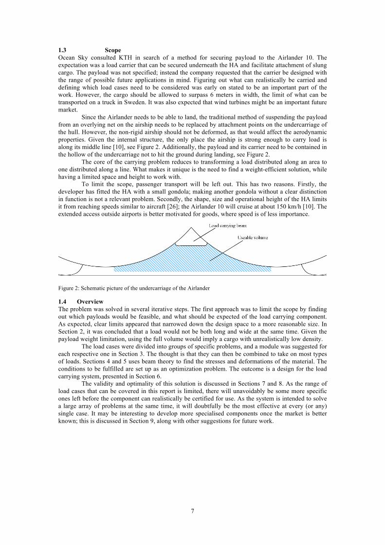
1.3 Scope Ocean Sky consulted KTH in search of a method for securing payload to the Airlander 10. The expectation was a load carrier that can be secured underneath the HA and facilitate attachment of slung cargo. The payload was not specified; instead the company requested that the carrier be designed with the range of possible future applications in mind. Figuring out what can realistically be carried and defining which load cases need to be considered was early on stated to be an important part of the work. However, the cargo should be allowed to surpass 6 meters in width, the limit of what can be transported on a truck in Sweden. It was also expected that wind turbines might be an important future market. Since the Airlander needs to be able to land, the traditional method of suspending the payload from an overlying net on the airship needs to be replaced by attachment points on the undercarriage of the hull. However, the non-rigid airship should not be deformed, as that would affect the aerodynamic properties. Given the internal structure, the only place the airship is strong enough to carry load is along its middle line [10], see Figure 2. Additionally, the payload and its carrier need to be contained in the hollow of the undercarriage not to hit the ground during landing, see Figure 2. The core of the carrying problem reduces to transforming a load distributed along an area to one distributed along a line. What makes it unique is the need to find a weight-efficient solution, while having a limited space and height to work with. To limit the scope, passenger transport will be left out. This has two reasons. Firstly, the developer has fitted the HA with a small gondola; making another gondola without a clear distinction in function is not a relevant problem. Secondly, the shape, size and operational height of the HA limits it from reaching speeds similar to aircraft [26]; the Airlander 10 will cruise at about 150 km/h [10]. The extended access outside airports is better motivated for goods, where speed is of less importance.

Figure 2: Schematic picture of the undercarriage of the Airlander

1.4 Overview The problem was solved in several iterative steps. The first approach was to limit the scope by finding out which payloads would be feasible, and what should be expected of the load carrying component. As expected, clear limits appeared that narrowed down the design space to a more reasonable size. In Section 2, it was concluded that a load would not be both long and wide at the same time. Given the payload weight limitation, using the full volume would imply a cargo with unrealistically low density.

The load cases were divided into groups of specific problems, and a module was suggested for each respective one in Section 3. The thought is that they can then be combined to take on most types of loads. Sections 4 and 5 uses beam theory to find the stresses and deformations of the material. The conditions to be fulfilled are set up as an optimization problem. The outcome is a design for the load carrying system, presented in Section 6.

The validity and optimality of this solution is discussed in Sections 7 and 8. As the range of load cases that can be covered in this report is limited, there will unavoidably be some more specific ones left before the component can realistically be certified for use. As the system is intended to solve a large array of problems at the same time, it will doubtfully be the most effective at every (or any) single case. It may be interesting to develop more specialised components once the market is better known; this is discussed in Section 9, along with other suggestions for future work.

8

2 Component requirements The carrying capabilities, limitations and costs are examined. This narrows the scope of the problem and allows for the determination of the types of cargo that might be feasible to carry.

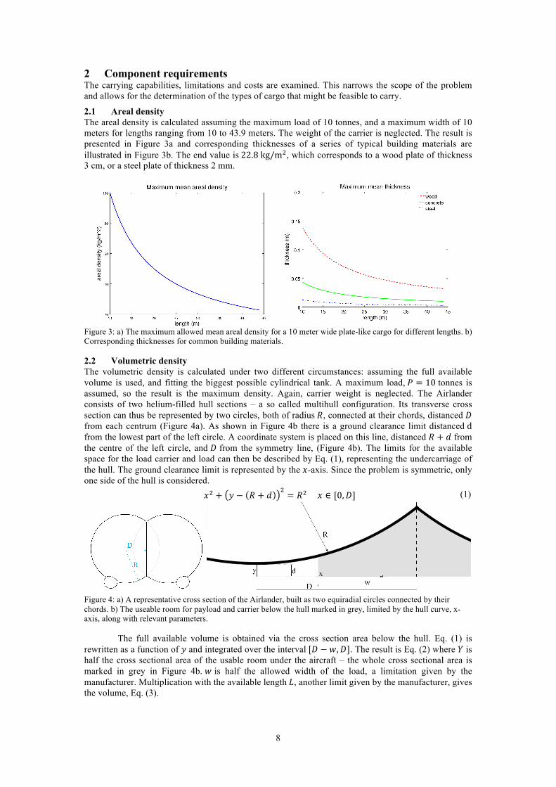
2.1 Areal density The areal density is calculated assuming the maximum load of 10 tonnes, and a maximum width of 10 meters for lengths ranging from 10 to 43.9 meters. The weight of the carrier is neglected. The result is presented in Figure 3a and corresponding thicknesses of a series of typical building materials are illustrated in Figure 3b. The end value is 22.8 kg/m!, which corresponds to a wood plate of thickness 3 cm, or a steel plate of thickness 2 mm.

Figure 3: a) The maximum allowed mean areal density for a 10 meter wide plate-like cargo for different lengths. b) Corresponding thicknesses for common building materials.

2.2 Volumetric density The volumetric density is calculated under two different circumstances: assuming the full available volume is used, and fitting the biggest possible cylindrical tank. A maximum load, 𝑃 = 10 tonnes is assumed, so the result is the maximum density. Again, carrier weight is neglected. The Airlander consists of two helium-filled hull sections – a so called multihull configuration. Its transverse cross section can thus be represented by two circles, both of radius 𝑅, connected at their chords, distanced 𝐷 from each centrum (Figure 4a). As shown in Figure 4b there is a ground clearance limit distanced d from the lowest part of the left circle. A coordinate system is placed on this line, distanced 𝑅 + 𝑑 from the centre of the left circle, and 𝐷 from the symmetry line, (Figure 4b). The limits for the available space for the load carrier and load can then be described by Eq. (1), representing the undercarriage of the hull. The ground clearance limit is represented by the 𝑥-axis. Since the problem is symmetric, only one side of the hull is considered. 𝑥! + 𝑦 − 𝑅 + 𝑑

!= 𝑅! 𝑥 ∈ [0,𝐷] (1)

Figure 4: a) A representative cross section of the Airlander, built as two equiradial circles connected by their chords. b) The useable room for payload and carrier below the hull marked in grey, limited by the hull curve, x-axis, along with relevant parameters.

The full available volume is obtained via the cross section area below the hull. Eq. (1) is rewritten as a function of 𝑦 and integrated over the interval [𝐷 − 𝑤,𝐷]. The result is Eq. (2) where 𝑌 is half the cross sectional area of the usable room under the aircraft – the whole cross sectional area is marked in grey in Figure 4b. 𝑤 is half the allowed width of the load, a limitation given by the manufacturer. Multiplication with the available length 𝐿, another limit given by the manufacturer, gives the volume, Eq. (3).

9

𝑌 = − 𝑅! − 𝑥! + 𝑅 + 𝑑 𝑑𝑥

!

!!! (2)

𝑉!"! = −𝐿 𝑅! − 𝑥! − 𝑅 + 𝑑 𝑑𝑥

!

!!! (3)

An alternative to using the full volume is only utilizing the volume that can be contained in a cylindrical tank. This is interesting due to the lower price of obtaining a cylindrical tank versus tailoring a form fitted tank for the aircraft. In this early estimate half the stated free height under the load carrying beam is used as a radius estimate. A more exact calculation on what the maximum radius of such a cylinder would be given the hull curvature can be found in Section 5.4.

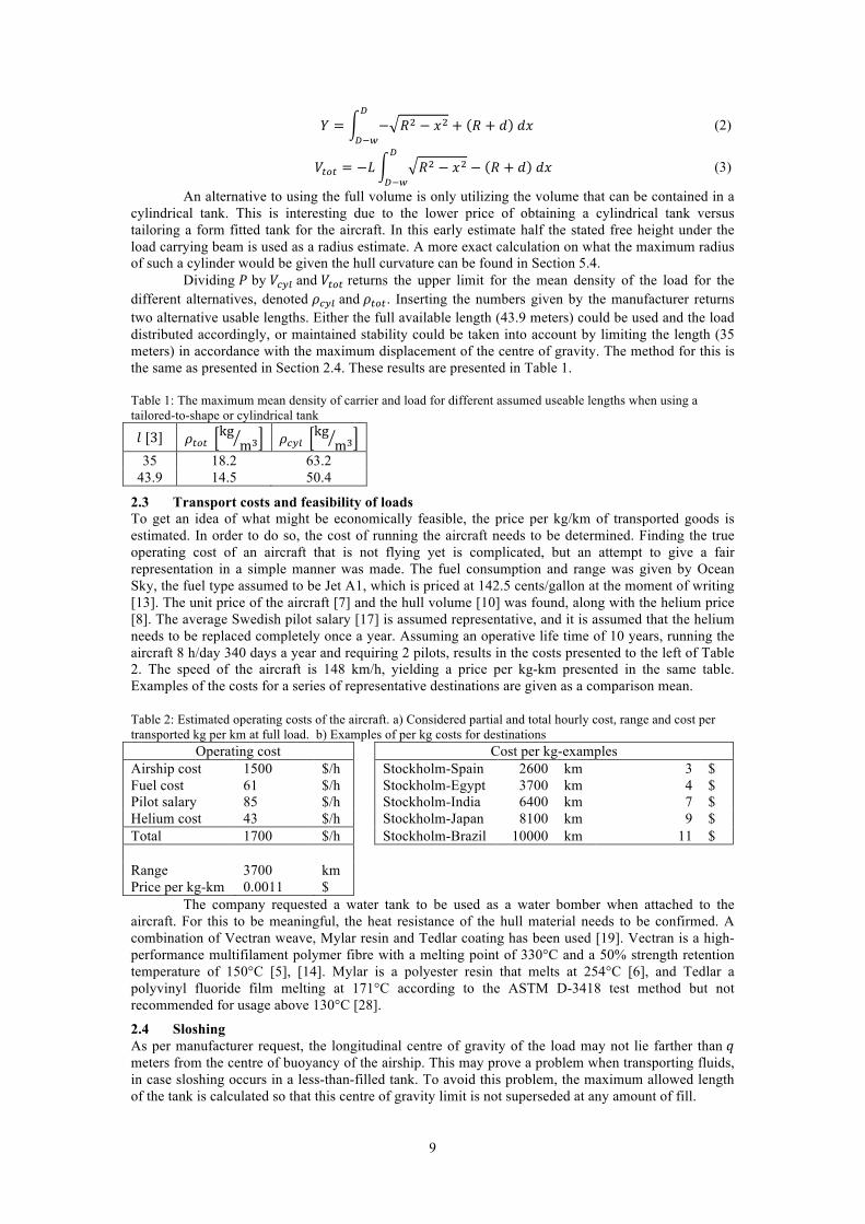
Dividing 𝑃 by 𝑉!"# and 𝑉!"! returns the upper limit for the mean density of the load for the different alternatives, denoted 𝜌!"# and 𝜌!"!. Inserting the numbers given by the manufacturer returns two alternative usable lengths. Either the full available length (43.9 meters) could be used and the load distributed accordingly, or maintained stability could be taken into account by limiting the length (35 meters) in accordance with the maximum displacement of the centre of gravity. The method for this is the same as presented in Section 2.4. These results are presented in Table 1.

Table 1: The maximum mean density of carrier and load for different assumed useable lengths when using a tailored-to-shape or cylindrical tank

𝑙 [3] 𝜌!"! kg m! 𝜌!"# kg m! 35 18.2 63.2

43.9 14.5 50.4

2.3 Transport costs and feasibility of loads To get an idea of what might be economically feasible, the price per kg/km of transported goods is estimated. In order to do so, the cost of running the aircraft needs to be determined. Finding the true operating cost of an aircraft that is not flying yet is complicated, but an attempt to give a fair representation in a simple manner was made. The fuel consumption and range was given by Ocean Sky, the fuel type assumed to be Jet A1, which is priced at 142.5 cents/gallon at the moment of writing [13]. The unit price of the aircraft [7] and the hull volume [10] was found, along with the helium price [8]. The average Swedish pilot salary [17] is assumed representative, and it is assumed that the helium needs to be replaced completely once a year. Assuming an operative life time of 10 years, running the aircraft 8 h/day 340 days a year and requiring 2 pilots, results in the costs presented to the left of Table 2. The speed of the aircraft is 148 km/h, yielding a price per kg-km presented in the same table. Examples of the costs for a series of representative destinations are given as a comparison mean.

Table 2: Estimated operating costs of the aircraft. a) Considered partial and total hourly cost, range and cost per transported kg per km at full load. b) Examples of per kg costs for destinations

Operating cost Cost per kg-examples Airship cost 1500 $/h Stockholm-Spain 2600 km 3 $ Fuel cost 61 $/h Stockholm-Egypt 3700 km 4 $ Pilot salary 85 $/h Stockholm-India 6400 km 7 $ Helium cost 43 $/h Stockholm-Japan 8100 km 9 $ Total 1700 $/h Stockholm-Brazil 10000 km 11 $ Range 3700 km Price per kg-km 0.0011 $ The company requested a water tank to be used as a water bomber when attached to the aircraft. For this to be meaningful, the heat resistance of the hull material needs to be confirmed. A combination of Vectran weave, Mylar resin and Tedlar coating has been used [19]. Vectran is a high-performance multifilament polymer fibre with a melting point of 330°C and a 50% strength retention temperature of 150°C [5], [14]. Mylar is a polyester resin that melts at 254°C [6], and Tedlar a polyvinyl fluoride film melting at 171°C according to the ASTM D-3418 test method but not recommended for usage above 130°C [28].

2.4 Sloshing As per manufacturer request, the longitudinal centre of gravity of the load may not lie farther than 𝑞 meters from the centre of buoyancy of the airship. This may prove a problem when transporting fluids, in case sloshing occurs in a less-than-filled tank. To avoid this problem, the maximum allowed length of the tank is calculated so that this centre of gravity limit is not superseded at any amount of fill.

10

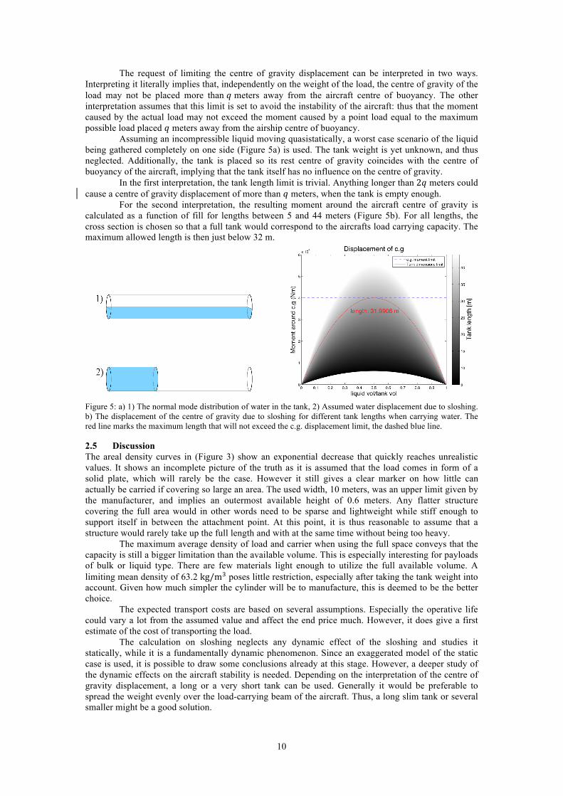
The request of limiting the centre of gravity displacement can be interpreted in two ways. Interpreting it literally implies that, independently on the weight of the load, the centre of gravity of the load may not be placed more than 𝑞 meters away from the aircraft centre of buoyancy. The other interpretation assumes that this limit is set to avoid the instability of the aircraft: thus that the moment caused by the actual load may not exceed the moment caused by a point load equal to the maximum possible load placed 𝑞 meters away from the airship centre of buoyancy. Assuming an incompressible liquid moving quasistatically, a worst case scenario of the liquid being gathered completely on one side (Figure 5a) is used. The tank weight is yet unknown, and thus neglected. Additionally, the tank is placed so its rest centre of gravity coincides with the centre of buoyancy of the aircraft, implying that the tank itself has no influence on the centre of gravity.

In the first interpretation, the tank length limit is trivial. Anything longer than 2𝑞 meters could cause a centre of gravity displacement of more than 𝑞 meters, when the tank is empty enough.

For the second interpretation, the resulting moment around the aircraft centre of gravity is calculated as a function of fill for lengths between 5 and 44 meters (Figure 5b). For all lengths, the cross section is chosen so that a full tank would correspond to the aircrafts load carrying capacity. The maximum allowed length is then just below 32 m.

Figure 5: a) 1) The normal mode distribution of water in the tank, 2) Assumed water displacement due to sloshing. b) The displacement of the centre of gravity due to sloshing for different tank lengths when carrying water. The red line marks the maximum length that will not exceed the c.g. displacement limit, the dashed blue line.

2.5 Discussion The areal density curves in (Figure 3) show an exponential decrease that quickly reaches unrealistic values. It shows an incomplete picture of the truth as it is assumed that the load comes in form of a solid plate, which will rarely be the case. However it still gives a clear marker on how little can actually be carried if covering so large an area. The used width, 10 meters, was an upper limit given by the manufacturer, and implies an outermost available height of 0.6 meters. Any flatter structure covering the full area would in other words need to be sparse and lightweight while stiff enough to support itself in between the attachment point. At this point, it is thus reasonable to assume that a structure would rarely take up the full length and with at the same time without being too heavy. The maximum average density of load and carrier when using the full space conveys that the capacity is still a bigger limitation than the available volume. This is especially interesting for payloads of bulk or liquid type. There are few materials light enough to utilize the full available volume. A limiting mean density of 63.2 kg/m! poses little restriction, especially after taking the tank weight into account. Given how much simpler the cylinder will be to manufacture, this is deemed to be the better choice. The expected transport costs are based on several assumptions. Especially the operative life could vary a lot from the assumed value and affect the end price much. However, it does give a first estimate of the cost of transporting the load. The calculation on sloshing neglects any dynamic effect of the sloshing and studies it statically, while it is a fundamentally dynamic phenomenon. Since an exaggerated model of the static case is used, it is possible to draw some conclusions already at this stage. However, a deeper study of the dynamic effects on the aircraft stability is needed. Depending on the interpretation of the centre of gravity displacement, a long or a very short tank can be used. Generally it would be preferable to spread the weight evenly over the load-carrying beam of the aircraft. Thus, a long slim tank or several smaller might be a good solution.

11

3 Proposed concept Using the results from the previous section, a chart of realistic load types was suggested (Figure 6). They were divided into three categories, wide loads, long loads and bulk loads, as it is expected that these will pose fundamentally different challenges to the load carrier. While large variation can be expected within each category further on, they are structurally similar at this early stage. Trying to solve all loads with one carrier is expected to be inefficient. Instead, the load carrier is designed in form of three different modules: one for wide payloads, one for long, slim payloads and one for bulk or liquid cargo. The idea is that they in need should be combinable: a load that is slim in one end and wide in the other can be attached with the two different modules. Similarly if a single large load needs to be carried together with something in bulk form, a short version of the bulk load tank can be manufactured and the large load attached with its respective module.

Figure 6: Diagram showing the realistic load types divided into three main categories. Wide loads, long loads and bulk loads that might need a container.

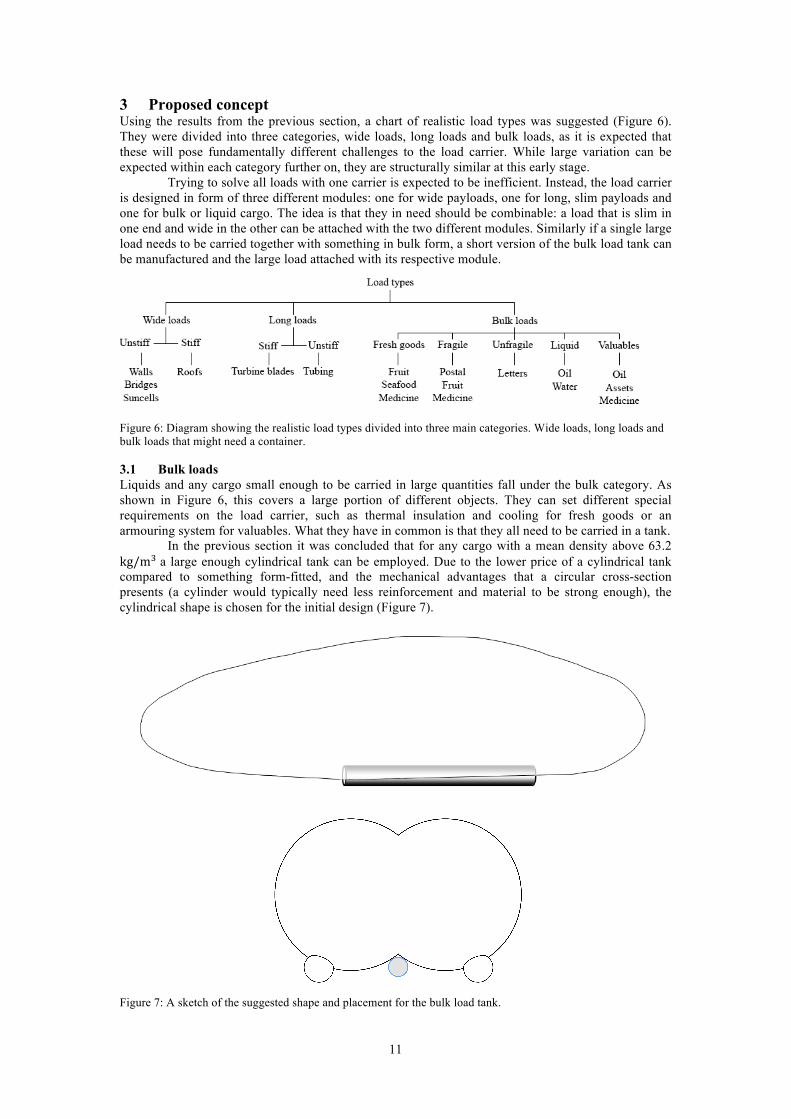
3.1 Bulk loads Liquids and any cargo small enough to be carried in large quantities fall under the bulk category. As shown in Figure 6, this covers a large portion of different objects. They can set different special requirements on the load carrier, such as thermal insulation and cooling for fresh goods or an armouring system for valuables. What they have in common is that they all need to be carried in a tank. In the previous section it was concluded that for any cargo with a mean density above 63.2 kg/m! a large enough cylindrical tank can be employed. Due to the lower price of a cylindrical tank compared to something form-fitted, and the mechanical advantages that a circular cross-section presents (a cylinder would typically need less reinforcement and material to be strong enough), the cylindrical shape is chosen for the initial design (Figure 7).

Figure 7: A sketch of the suggested shape and placement for the bulk load tank.

12

Given the expected low cost of cylindrical structures, a company could keep several tanks. Different tanks can be modified for the specific constraints set by different types of bulk load, further decreasing the complexity of each cylinder and allowing to always choose the lightest and most appropriate tank for the type cargo at hand.

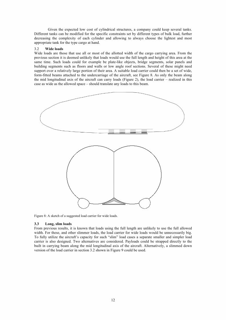
3.2 Wide loads Wide loads are those that use all or most of the allotted width of the cargo carrying area. From the previous section it is deemed unlikely that loads would use the full length and height of this area at the same time. Such loads could for example be plate-like objects, bridge segments, solar panels and building segments such as floors and walls or low angle roof sections. Several of these might need support over a relatively large portion of their area. A suitable load carrier could then be a set of wide, form-fitted beams attached to the undercarriage of the aircraft, see Figure 8. As only the beam along the mid longitudinal axis of the aircraft can carry loads (Figure 2), the load carrier – realized in this case as wide as the allowed space – should translate any loads to this beam.

Figure 8: A sketch of a suggested load carrier for wide loads.

3.3 Long, slim loads From previous results, it is known that loads using the full length are unlikely to use the full allowed width. For these, and other slimmer loads, the load carrier for wide loads would be unnecessarily big. To fully utilize the aircraft’s capacity for such “slim” load cases a separate smaller and simpler load carrier is also designed. Two alternatives are considered. Payloads could be strapped directly to the built in carrying beam along the mid longitudinal axis of the aircraft. Alternatively, a slimmed down version of the load carrier in section 3.2 shown in Figure 9 could be used.

13

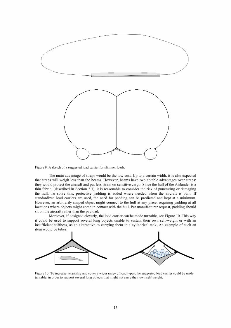
Figure 9: A sketch of a suggested load carrier for slimmer loads.

The main advantage of straps would be the low cost. Up to a certain width, it is also expected that straps will weigh less than the beams. However, beams have two notable advantages over straps: they would protect the aircraft and put less strain on sensitive cargo. Since the hull of the Airlander is a thin fabric, (described in Section 2.3), it is reasonable to consider the risk of puncturing or damaging the hull. To solve this, protective padding is added where needed when the aircraft is built. If standardized load carriers are used, the need for padding can be predicted and kept at a minimum. However, an arbitrarily shaped object might connect to the hull at any place, requiring padding at all locations where objects might come in contact with the hull. Per manufacturer request, padding should sit on the aircraft rather than the payload.

Moreover, if designed cleverly, the load carrier can be made turnable, see Figure 10. This way it could be used to support several long objects unable to sustain their own self-weight or with an insufficient stiffness, as an alternative to carrying them in a cylindrical tank. An example of such an item would be tubes.

Figure 10: To increase versatility and cover a wider range of load types, the suggested load carrier could be made turnable, in order to support several long objects that might not carry their own self-weight.

14

4 Theory To determine the necessary dimensions of the load carriers suggested in Section 3 a stress and deformation analysis is performed. Assuming a certain set of dimensional parameters, their relations to the structural response and internal stresses derived for different load conditions. Care is taken to keep equations in analytic form, to allow for optimization or testing of different parameters later on.

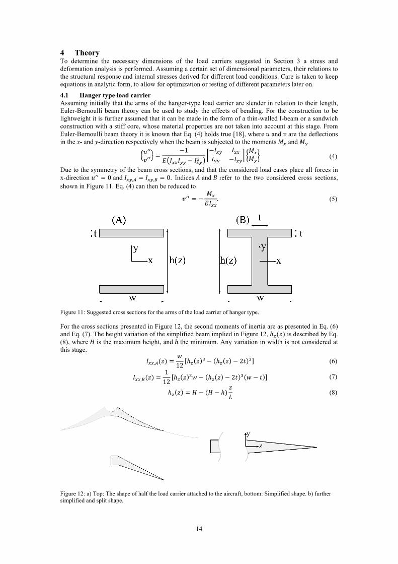
4.1 Hanger type load carrier Assuming initially that the arms of the hanger-type load carrier are slender in relation to their length, Euler-Bernoulli beam theory can be used to study the effects of bending. For the construction to be lightweight it is further assumed that it can be made in the form of a thin-walled I-beam or a sandwich construction with a stiff core, whose material properties are not taken into account at this stage. From Euler-Bernoulli beam theory it is known that Eq. (4) holds true [18], where 𝑢 and 𝑣 are the deflections in the x- and y-direction respectively when the beam is subjected to the moments 𝑀! and 𝑀! 𝑢′′

𝑣′′=

−1𝐸 𝐼!!𝐼!! − 𝐼!"!

−𝐼!" 𝐼!!𝐼!! −𝐼!"

𝑀!𝑀!

(4)

Due to the symmetry of the beam cross sections, and that the considered load cases place all forces in x-direction 𝑢!! = 0 and 𝐼!",! = 𝐼!",! = 0. Indices 𝐴 and 𝐵 refer to the two considered cross sections, shown in Figure 11. Eq. (4) can then be reduced to

𝑣!! = −𝑀!

𝐸𝐼!!. (5)

Figure 11: Suggested cross sections for the arms of the load carrier of hanger type.

For the cross sections presented in Figure 12, the second moments of inertia are as presented in Eq. (6) and Eq. (7). The height variation of the simplified beam implied in Figure 12, ℎ!(𝑧) is described by Eq. (8), where 𝐻 is the maximum height, and ℎ the minimum. Any variation in width is not considered at this stage. 𝐼!!,!(𝑧) =

𝑤12

ℎ! 𝑧 ! − ℎ! 𝑧 − 2𝑡 ! (6)

𝐼!!,!(𝑧) =

112

ℎ! 𝑧 !𝑤 − ℎ! 𝑧 − 2𝑡 ! 𝑤 − 𝑡 (7)

ℎ! 𝑧 = 𝐻 − (𝐻 − ℎ)𝑧𝐿

(8)

Figure 12: a) Top: The shape of half the load carrier attached to the aircraft, bottom: Simplified shape. b) further simplified and split shape.

15

Due to symmetry, only one side of the load carrier is considered in the calculations. The load carrier is attached to the aircraft where beam has been split. It can thus be treated as a full-moment-connected cantilever beam. The analysis focuses on the tapered part of the beam only. Partly because the other is shorter and supported at both ends, thus expected to sustain loads better, and partly since less of the constricting dimensions are known for certain. The stress due to this bending is given by Eq. (9), which is reduced to Eq. (10). Due to the original angle of the beam, in the left of Figure 12, an axial load component is expected giving the stress component in Eq. (11). Additionally there will be a shear stress component, described by Eq. (12) [18]. The force is applied at an angle on the simplified shape, meaning that 𝑃 = 𝐹 sin(𝛼) is the axial force, and 𝑇 = 𝐹 cos(𝛼). Further, the cross section area is projected at an angle in the simplified shape giving a new area 𝐴/ cos(𝛼) used in Eq. (11)-(12)

𝜎!,!"#$(𝑧) =𝑀!𝐼!! −𝑀!𝐼!"𝐼!!𝐼!! − 𝐼!"!

𝑥 +𝑀!𝐼!! −𝑀!𝐼!"𝐼!!𝐼!! − 𝐼!"!

𝑦 (9)

𝜎!,!"#$(𝑧) =

𝑀!

𝐼!!𝑦 (10)

𝜎!,!"#!$ =

𝑃 cos 𝛼𝐴

(11)

𝜏!" =

𝑇 cos 𝛼𝐴

(12)

The resulting shear is found using the reduced von Mises equivalent stress in Eq. (13). This reduces to Eq. (14) since 𝜎! = 𝜎! = 𝜏!" = 𝜏!" = 0. The stress components in the z-direction are summed.

𝜎! =32𝑠!"𝑠!"

!!=

12𝜎!! + 𝜎!! + 𝜎!! − 𝜎!𝜎! − 𝜎!𝜎! − 𝜎!𝜎! + 3𝜏!"! + 3𝜏!" + 3𝜏!" (13)

𝜎! =

12𝜎!! + 3𝜏!"! (14)

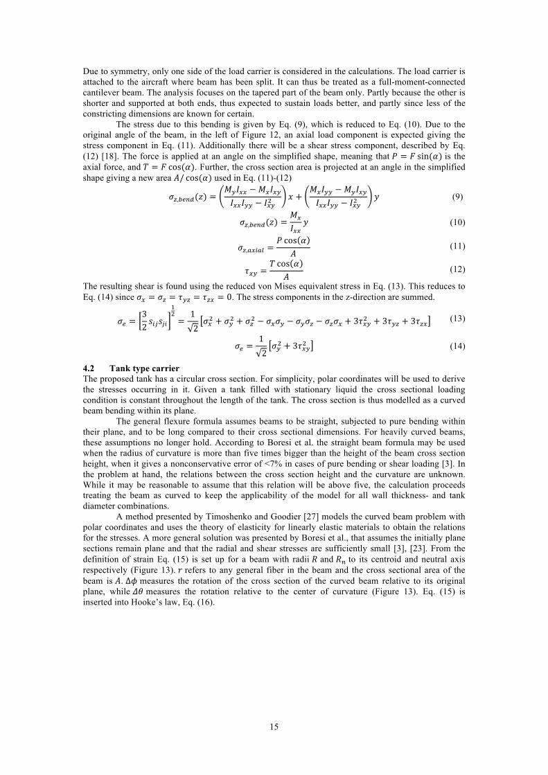
4.2 Tank type carrier The proposed tank has a circular cross section. For simplicity, polar coordinates will be used to derive the stresses occurring in it. Given a tank filled with stationary liquid the cross sectional loading condition is constant throughout the length of the tank. The cross section is thus modelled as a curved beam bending within its plane. The general flexure formula assumes beams to be straight, subjected to pure bending within their plane, and to be long compared to their cross sectional dimensions. For heavily curved beams, these assumptions no longer hold. According to Boresi et al. the straight beam formula may be used when the radius of curvature is more than five times bigger than the height of the beam cross section height, when it gives a nonconservative error of <7% in cases of pure bending or shear loading [3]. In the problem at hand, the relations between the cross section height and the curvature are unknown. While it may be reasonable to assume that this relation will be above five, the calculation proceeds treating the beam as curved to keep the applicability of the model for all wall thickness- and tank diameter combinations.

A method presented by Timoshenko and Goodier [27] models the curved beam problem with polar coordinates and uses the theory of elasticity for linearly elastic materials to obtain the relations for the stresses. A more general solution was presented by Boresi et al., that assumes the initially plane sections remain plane and that the radial and shear stresses are sufficiently small [3], [23]. From the definition of strain Eq. (15) is set up for a beam with radii 𝑅 and 𝑅! to its centroid and neutral axis respectively (Figure 13). 𝑟 refers to any general fiber in the beam and the cross sectional area of the beam is 𝐴. ∆𝜙 measures the rotation of the cross section of the curved beam relative to its original plane, while 𝛥𝜃 measures the rotation relative to the center of curvature (Figure 13). Eq. (15) is inserted into Hooke’s law, Eq. (16).

16

Figure 13: Representative section of a curved beam with dimensions and applied forces [23].

𝜀!! =

∆𝑙𝑙=

𝑅! − 𝑟 ∆𝜙𝑟∆𝜃

(15)

𝜎!! = 𝐸𝜀!! (16) Given the above, the following relations can be set up for the normal force, 𝑁, and moment, 𝑀.

𝑁 = 𝜎!!𝑑𝐴 = 𝐸∆𝜙∆𝜃

(𝑅!𝐴! − 𝐴)

!

(17)

𝑀 = 𝜎!! 𝑅 − 𝑟 𝑑𝐴 = 𝐸𝑅!

∆𝜙∆𝜃

(𝑅𝐴! − 𝐴)

!

(18)

where 𝐴! has the dimension length and is introduced to simplify the expression. The form of the expression for 𝐴! depends on the beam cross section, and is listed for different cases by Boresi et al..

𝐴! =𝑑𝐴𝑟.

!

(19)

Rewriting Eq. (17) as a function of 𝐸 ∆!∆!𝑅! yields Eq. (20). Insertion of this, and reformulation of Eq.

(18) as a function of 𝐸 ∆!∆!

then gives Eq. (21).

𝐸∆𝜙∆𝜃

𝑅! =𝑀

𝑅𝐴! − 𝐴 (20)

𝐸∆𝜙∆𝜃

=𝑀𝐴!

𝐴 𝑅𝐴! − 𝐴 (21)

Revisiting Eq. (15)-(16), the stress can be reformulated as Eq. (22).

𝜎!! = 𝐸∆𝜙∆𝜃

𝑅! − 𝑟𝑟

=𝐸 ∆𝜙𝑟∆𝜃 𝑅!𝑟

− 𝐸∆𝜙𝑟∆𝜃

(22)

Insertion of Eq. (20)-(21) finally yields an expression for the stress as a function of the dimensions and applied forces in Eq. (23).

𝜎!! =𝑁𝐴+𝑀 𝐴 − 𝑟𝐴!𝐴𝑟(𝑅𝐴! − 𝐴)

(23)

17

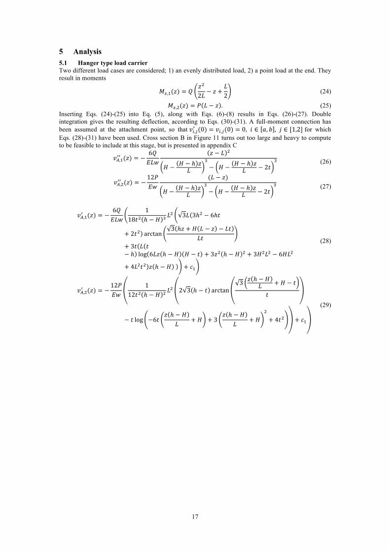
5 Analysis 5.1 Hanger type load carrier Two different load cases are considered; 1) an evenly distributed load, 2) a point load at the end. They result in moments

𝑀!,!(𝑧) = 𝑄𝑧!

2𝐿− 𝑧 +

𝐿2

(24)

𝑀!,!(𝑧) = 𝑃 𝐿 − 𝑧 . (25) Inserting Eqs. (24)-(25) into Eq. (5), along with Eqs. (6)-(8) results in Eqs. (26)-(27). Double integration gives the resulting deflection, according to Eqs. (30)-(31). A full-moment connection has been assumed at the attachment point, so that 𝑣!,!! (0) = 𝑣!,!(0) = 0, 𝑖 ∈ 𝑎, 𝑏 , 𝑗 ∈ [1,2] for which Eqs. (28)-(31) have been used. Cross section B in Figure 11 turns out too large and heavy to compute to be feasible to include at this stage, but is presented in appendix C

𝑣!,!!! (𝑧) = −6𝑄𝐸𝐿𝑤

𝑧 − 𝐿 !

𝐻 − 𝐻 − ℎ 𝑧𝐿

!− 𝐻 − 𝐻 − ℎ 𝑧

𝐿 − 2𝑡! (26)

𝑣!,!!! (𝑧) = −

12𝑃𝐸𝑤

(𝐿 − 𝑧)

𝐻 − 𝐻 − ℎ 𝑧𝐿

!− 𝐻 − 𝐻 − ℎ 𝑧

𝐿 − 2𝑡! (27)

𝑣!,!! (𝑧) = −6𝑄𝐸𝐿𝑤

118𝑡! ℎ − 𝐻 ! 𝐿

! 3𝐿 3ℎ! − 6ℎ𝑡

+ 2𝑡! arctan3 ℎ𝑧 + 𝐻 𝐿 − 𝑧 − 𝐿𝑡

𝐿𝑡+ 3𝑡 𝐿 𝑡− ℎ log 6𝐿𝑧 ℎ − 𝐻 𝐻 − 𝑡 + 3𝑧! ℎ − 𝐻 ! + 3𝐻!𝐿! − 6𝐻𝐿!

+ 4𝐿!𝑡! 𝑧 ℎ − 𝐻 + 𝑐!

(28)

𝑣!,!! (𝑧) = −12𝑃𝐸𝑤

112𝑡! ℎ − 𝐻 ! 𝐿

! 2 3 ℎ − 𝑡 arctan3 𝑧 ℎ − 𝐻

𝐿 + 𝐻 − 𝑡

𝑡

− 𝑡 log −6𝑡𝑧 ℎ − 𝐻

𝐿+ 𝐻 + 3

𝑧 ℎ − 𝐻𝐿

+ 𝐻!

+ 4𝑡! + 𝑐!

(29)

18

𝑣!,!(𝑧)

= −6𝑄𝐸𝐿𝑤

136𝑡! ℎ − 𝐻 ! 𝐿

! −3ℎ!𝐿!𝑡 − 6ℎ𝐻𝐿!𝑡 + 12ℎ𝐿!𝑡! + 6𝐻𝐿!𝑡!

− 8𝐿!𝑡! log 3ℎ!𝑧! + 6ℎ𝐻𝐿𝑧 − 6ℎ𝐻𝑧! − 6ℎ𝐿𝑡𝑧 + 3𝐻!𝐿! − 6𝐻!𝐿𝑧 + 3𝐻!𝑧! − 6𝐻𝐿!𝑡+ 6𝐻𝐿𝑡𝑧𝑧 + 4𝐿!𝑡!

−𝐿!𝑧 ℎ − 𝑡 log 3ℎ!𝑧! − 6𝐻 𝐿 − 𝑧 𝐿𝑡 − ℎ𝑧 − 6ℎ𝐿𝑡𝑧 + 3𝐻! 𝐿 − 𝑧 ! + 4𝐿!𝑡!

6𝑡 ℎ − 𝐻 !

−𝐿! 3ℎ!𝐻 − 3ℎ!𝑡 − 6ℎ𝐻𝑡 + 4ℎ𝑡! + 2𝐻𝑡! arctan 3 −ℎ𝑧 − 𝐻𝐿 + 𝐻𝑧 + 𝐿𝑡

𝐿𝑡

6 3𝑡! ℎ − 𝐻 !

+𝐿!𝑧 3ℎ! − 6ℎ𝑡 + 2𝑡! arctan 3 ℎ𝑧 + 𝐻𝐿 − 𝐻𝑧 − 𝐿𝑡

𝐿𝑡

6 3𝑡! ℎ − 𝐻 ! +𝐿!𝑧 ℎ − 𝑡3𝑡 ℎ − 𝐻 ! +

𝐿!𝑧!

12𝑡 ℎ − 𝐻 !

+ 𝑐!𝑧 + 𝑐!

(30)

𝑣!,!(𝑧)

= −12𝑃𝐸𝑤

136

−3𝐿! ℎ − 2𝑡 log −6𝑡 𝑧 ℎ − 𝐻

𝐿 + 𝐻 + 3 𝑧 ℎ − 𝐻𝐿 + 𝐻

!+ 4𝑡!

𝑡 ℎ − 𝐻 !

+

2 3𝐿! 2𝑡 − 3ℎ arctan3 𝑧 ℎ − 𝐻

𝐿 + 𝐻 − 𝑡𝑡

𝑡 ℎ − 𝐻 !

−3𝐿! ℎ𝑧 + 𝐻 𝐿 − 𝑧 log −6𝑡 𝑧 ℎ − 𝐻

𝐿 + 𝐻 + 3 𝑧 ℎ − 𝐻𝐿 + 𝐻

!+ 4𝑡!

𝑡 ℎ − 𝐻 !

+

6 3𝐿! ℎ − 𝑡 ℎ𝑧 + 𝐻 𝐿 − 𝑧 arctan3 𝑧 ℎ − 𝐻

𝐿 + 𝐻 − 𝑡𝑡

𝑡! ℎ − 𝐻 ! +6𝐿! ℎ𝑧 + 𝐻 𝐿 − 𝑧

𝑡 ℎ − 𝐻 !

+ 𝑐! + 𝑐!

(31)

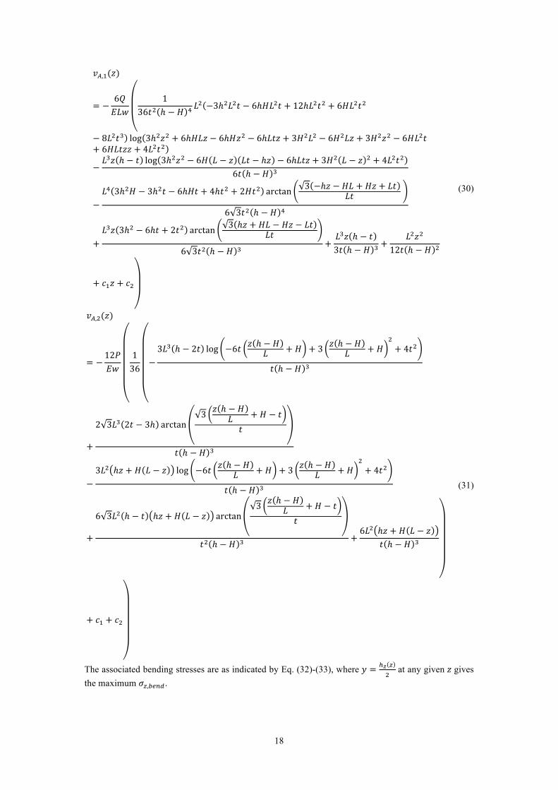
The associated bending stresses are as indicated by Eq. (32)-(33), where 𝑦 = !! !!

at any given 𝑧 gives the maximum 𝜎!,!"#$.

19

𝜎!,!"#$,!,!(𝑧) = −

6𝑄𝐿𝑤

𝑧 − 𝐿 !

𝐻 − 𝐻 − ℎ 𝑧𝐿

!− 𝐻 − 𝐻 − ℎ 𝑧

𝐿 − 2𝑡! 𝑦 (32)

𝜎!,!"#$,!,!(𝑧) = −

12𝑃𝑤

(𝐿 − 𝑧)

𝐻 − 𝐻 − ℎ 𝑧𝐿

!− 𝐻 − 𝐻 − ℎ 𝑧

𝐿 − 2𝑡! 𝑦 (33)

The axial stress is a simple function of area as given by Eq. (34) which leads to Eq. (36). The shear stress is described by Eq. (37)-(38). 𝐴! = 2𝑡𝑤 (34)

𝜎!,!"#!$,! =𝑃 sin 𝜁𝐴!

(35)

𝜏!",!,! =𝑄𝑧𝐴!𝐿

(37)

𝜏!",!,! =𝑃𝐴!

(38)

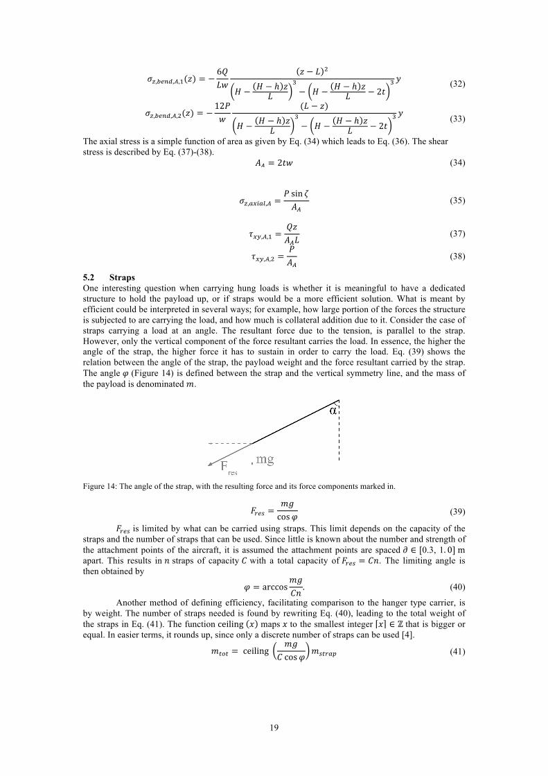
5.2 Straps One interesting question when carrying hung loads is whether it is meaningful to have a dedicated structure to hold the payload up, or if straps would be a more efficient solution. What is meant by efficient could be interpreted in several ways; for example, how large portion of the forces the structure is subjected to are carrying the load, and how much is collateral addition due to it. Consider the case of straps carrying a load at an angle. The resultant force due to the tension, is parallel to the strap. However, only the vertical component of the force resultant carries the load. In essence, the higher the angle of the strap, the higher force it has to sustain in order to carry the load. Eq. (39) shows the relation between the angle of the strap, the payload weight and the force resultant carried by the strap. The angle 𝜑 (Figure 14) is defined between the strap and the vertical symmetry line, and the mass of the payload is denominated 𝑚.

Figure 14: The angle of the strap, with the resulting force and its force components marked in.

𝐹!"# =𝑚𝑔cos𝜑

(39)

𝐹!"# is limited by what can be carried using straps. This limit depends on the capacity of the straps and the number of straps that can be used. Since little is known about the number and strength of the attachment points of the aircraft, it is assumed the attachment points are spaced 𝜕 ∈ [0.3, 1. 0] m apart. This results in 𝑛 straps of capacity 𝐶 with a total capacity of 𝐹!"# = 𝐶𝑛. The limiting angle is then obtained by 𝜑 = arccos

𝑚𝑔𝐶𝑛

. (40)

Another method of defining efficiency, facilitating comparison to the hanger type carrier, is by weight. The number of straps needed is found by rewriting Eq. (40), leading to the total weight of the straps in Eq. (41). The function ceiling 𝑥 maps 𝑥 to the smallest integer 𝑥 ∈ ℤ that is bigger or equal. In easier terms, it rounds up, since only a discrete number of straps can be used [4]. 𝑚!"! = ceiling

𝑚𝑔𝐶 cos𝜑

𝑚!"#$% (41)

20

5.3 Tank type carrier

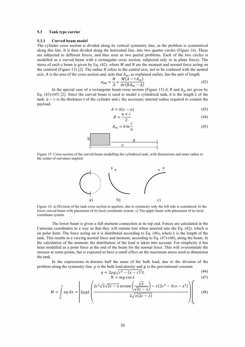
5.3.1 Curved beam model The cylinder cross section is divided along its vertical symmetry line, as the problem is symmetrical along this line. It is then divided along the horizontal line, into two quarter circles (Figure 16). These are subjected to different forces, and thus seen as two partial problems. Each of the two circles is modelled as a curved beam with a rectangular cross section, subjected only to in plane forces. The stress of such a beam is given by Eq. (42), where 𝑀 and 𝑁 are the moment and normal force acting on the centroid (Figure 13) [2]. The radius 𝑅 refers to the central axis, not to be confused with the neutral axis. 𝐴 is the area of the cross section and, note that 𝐴!, as explained earlier, has the unit of length.

𝜎!! =𝑁𝐴+𝑀 𝐴 − 𝑟𝐴!𝐴𝑟 𝑅𝐴! − 𝐴

(42)

In the special case of a rectangular beam cross section (Figure 15) 𝐴, 𝑅 and 𝐴! are given by Eq. (43)-(45) [2]. Since the curved beam is used to model a cylindrical tank, 𝑏 is the length 𝐿 of the tank. 𝑎 − 𝑐 is the thickness 𝑡 of the cylinder and 𝑐 the necessary internal radius required to contain the payload. 𝐴 = 𝑏(𝑐 − 𝑎) (43)

𝑅 =𝑎 + 𝑐2

(44)

𝐴! = 𝑏 ln𝑐𝑎

(45)

Figure 15: Cross section of the curved beam modelling the cylindrical tank, with dimensions and inner radius to the center of curvature implied.

Figure 16: a) Division of the tank cross section in quarters, due to symmetry only the left side is considered. b) the lower curved beam with placement of its local coordinate system. c) The upper beam with placement of its local coordinate system.

The lower beam is given a full moment connection at its top end. Forces are calculated in the Cartesian coordinates in a way so that they will remain true when inserted into the Eq. (42), which is on polar form. The force acting on it is distributed according to Eq. (46), where 𝐿 is the length of the tank. This results in a varying normal force and moment, according to Eq. (47)-(48), along the beam. In the calculation of the moment, the distribution of the load is taken into account. For simplicity it has been modelled as a point force at the end of the beam for the normal force. This will overestimate the stresses at some points, but is expected to have a small effect on the maximum stress used to dimension the tank.

In the expressions, 𝑚 denotes half the mass of the bulk load, due to the division of the problem along the symmetry line. 𝜌 is the bulk load density and 𝑔 is the gravitational constant. 𝑞 = 2𝜌𝑔 𝑐! − 𝑥 − 𝑐 !𝐿 (46) 𝑁 = 𝑚𝑔 cos 𝑥 (47)

𝑀 = 𝑥𝑞 𝑑𝑥!

!

= 2𝜌𝑔𝐿2𝑐! 𝑥 2𝑐 − 𝑥 arctan 𝑥

2𝑐 − 𝑥− 𝑥 2𝑐! − 3𝑐𝑥 − 𝑥!

2 𝑥 2𝑐 − 𝑥

!

!

(48)

21

Due to symmetry and attachment conditions, the top end of upper beam can be modelled as a full-moment connection. The weight of the bulk load will be distributed along the lower beam, so the only force acting on it will be a normal force and a moment at the end, given by Eq. (49)-(50). 𝑁 = 𝑚𝑔 sin 𝑥 (49)

𝑀 = 𝑥𝑞 𝑑𝑥!

!

+𝑚𝑔𝑥 cos 𝑥 = 2𝜌𝑔𝐿 𝑐! arctan 𝑥 + 𝑐! +𝑚𝑔𝑥 cos 𝑥 (50)

5.3.2 Pressurized tank model The cylinder tank is also examined using an alternative method; modelling it as a pressurized tube. For a thin-walled cylindrical pressurized tank with an internal pressure 𝑝, mean radius 𝑎 and wall thickness ℎ the principal stresses, in polar coordinates are given by Eq. (51)-(53) and the maximum shear by Eq. (54) [16]. 𝜎! ≈ 0 (51) 𝜎! =

𝑝𝑎2ℎ

(52) 𝜎! =

𝑝𝑎ℎ

(53) 𝜏!"# =

𝑝𝑎2ℎ

(54) The internal pressure is assumed to be equal to the weight of the tallest water column, according to Eq. (55). 𝑝 = 𝜌𝑔ℎ. (55)

5.3.3 Isotropic material failure criteria The failure criteria used for the isotropic materials examined (metals, plastics) was the comparison of the principal stresses (Eq. (51)-(53)) and shear (Eq. (54)) to the tensile- and shear strength of the material. The margin of safety was defined using this relation. The material properties of the materials considered are listed in Table 3 [1], [21], [22], [31]. Table 3: Material properties of considered isotropic materials. Material Tensile strength [MPa] Density [kg/m3] Aluminium 255 2700 Acrylic 55 1410 Acetal 66 1180 Epoxy 60 1200

5.3.4 Composite material failure criteria For simplicity, unidirectional layers have been assumed for the composite tanks. The failure criteria used was the maximum stress in each of the layers to find the first ply failure. The stresses occurring in each of the layers are not equal to the global stress resultants listed in Eq. (51)-(53). As the plies cannot deform independently, they all have the same global strain, that depending on the fibre orientation on the individual layers will result in different stresses. The calculation of the stresses is done similarly to an example given in [30].

Figure 17: Local lamina coordinates [2].

For a given type of lamina, i.e. unidirectional layer of fibre-matrix combination, the local stiffness matrix 𝑸𝒍 is given by Eq. (56), where 𝜈!" is given by Eq. (57). The local coordinate system is defined with the 1-direction running alongside the fibers, 2-direction perpendicular to them in the plane (Figure 17).

𝑸𝒍 =1

1 − 𝜈!"𝜈!"

𝐸! 𝜈!"𝐸! 0𝜈!"𝐸! 𝐸! 00 0 𝐺!"(1 − 𝜈!"𝜈!")

(56)

22

𝜈!" =𝜈!"𝐸!𝐸!

(57)

Each of these local stiffness matrices can then be transformed into a common global coordinate system. This is done according to Eq. (58) where the transformation matrix 𝑻 is given by Eq. (59)-(61). 𝜃 is the angle of rotation of the coordinate system, i.e. the angle of the fibres in the global coordinates. 𝑸 = 𝑻𝑸𝒍𝑻𝒕 (58)

𝑻 =𝑐! 𝑠! −2𝑠𝑐𝑠! 𝑐! 2𝑠𝑐𝑠𝑐 −𝑠𝑐 𝑐! − 𝑠!

(59)

𝑐 = cos 𝜃 (60) 𝑠 = sin 𝜃 (61) The stiffness of the laminate, i.e. all the lamina attached together, can be represented by the extensional stiffness matrix 𝑨, described by Eq. (61). The index 𝑖 identifies each of the layers in the laminate. Using Eq. (63), the global stress resultants found in Eq. (51)-(53) or Eq. (23) or can be used to find the global strains 𝜺 in the laminate, since 𝑁 depends directly on 𝜎 according to Eq. (64).

𝑨 = 𝑸𝒊ℎ!

!

!!!

(62)

𝜺 = 𝑨!𝟏𝑵 (63)

𝑵 = 𝝈

!!

!!!

𝑑𝑧 (64)

After transforming the global strains into the local strains 𝜺𝒍 using Eq. (65), the local stresses 𝝈𝒍 can finally be found using Eq. (66). 𝜺𝒍 = 𝑻𝒕𝜺 (65) 𝝈𝒍 = 𝑸𝒍𝜺𝒍 (66) The first failure criteria used is the maximum stress criteria. It states that none of the principal direction stresses may exceed the respective strengths Eq. (67)-(69) [30]. 𝜎!" , 𝜎!" represent the tensile and compressive strength in the 𝑖-direction where 𝑖 ∈ [1,2] and 𝜏!" is the shear strength. −𝜎!! < 𝜎! < 𝜎!! (67) −𝜎!! < 𝜎! < 𝜎!! (68) 𝜏!" < 𝜏!" (69) Similarly to the maximum stress criteria, the maximum strain criteria compares the strains in the principal directions to the ultimate strains in the same directions according to equations 70-72. −𝜀!! < 𝜀! < 𝜀!! (70) −𝜀!! < 𝜀! < 𝜀!! (71) 𝛾!" < 𝛾!" (72) The third failure criteria considered is the Tsai-Hill (Eq. (73)). While the maximum strain and stress give a rectangular failure envelope, assuming that the material never breaks unless the principal ultimate stresses or strains are reached, the Tsai-Hill criteria gives an elliptical failure envelope. The form of the equation is a simplified one only valid for laminas where a state of plane stress can be assumed. This criteria does not consider whether the stresses are compressive or tensile, and thus has limited accuracy for materials where these strengths differ. 𝜎!!

𝜎!!−𝜎!𝜎!𝜎!!

+𝜎!!

𝜎!!+𝜏!"!

𝜏!"!= 1 (73)

The material properties of the composites considered in this study are taken from a table listing typical parameters of laminas with different fibre reinforcement [30]. Used data is listed in Table 4. Table 4: Typical material parameters for laminas with considered unidirectional fibre reinforcement Lamina fibre

ℎ! [mm] 𝜌 [kg/m!] 𝐸! [GPa] 𝐸! [GPa] 𝐺!" [GPa] 𝜈!" 𝜎!! [MPa] 𝜎!! [MPa] 𝜎!! [MPa]

E-glass 0.127 1940 40 9.8 2.8 0.3 1100 600 20 Carbon 0.127 1500 147 9 3.3 0.31 2260 1200 50

Lamina fibre

𝜎!! [MPa] 𝜏!" [MPa] 𝜀!! 𝜀!! 𝜀!! 𝜀!! 𝛾!"

E-glass 140 70 0.028 0.015 0.002 0.014 0.014 Carbon 190 100 0.015 0.008 0.005 0.021 0.030

23

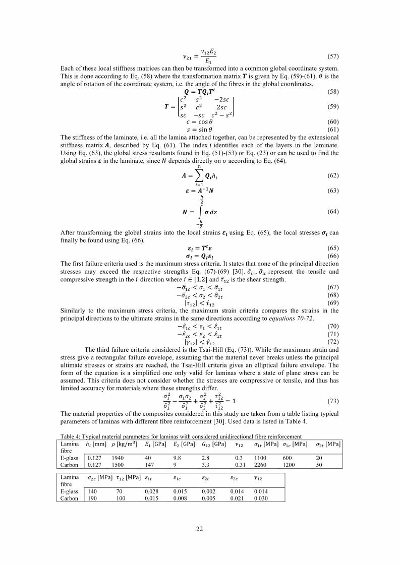
5.4 Cylinder size constraint

Figure 18: The useable room for payload and carrier under the hull marked in grey, along with relevant curves and parameters in black. The equilateral and right-angled triangles are used to determine the radii 𝒓 corresponding to each or the points on line 1. The smallest of these 𝒓 describes the biggest circle that would fit in the room.

Due to the shape of the undercarriage of the aircraft, the upper radius limit of something carried below it is not a direct function of the free height in the middle. In order to determine the exact dimensional constraints for cylindrical tanks, this upper radius limit needs to be determined. In other words, the biggest circle fitting into the cross-sectional area below the hull needs to be determined. It is clear, due to the symmetry and slope, that the best placement of this circle is on the symmetry line, as indicated in grey in Figure 18. This hypothetical circle, of radius 𝑟, is defined by Eq. (74). 𝑥 − 𝐷 ! + 𝑦 − 𝑟 ! = 𝑟! (74) This curve should be tangent to the one defined by Eq. (1), rewritten in Eq. (81), and to the 𝑥-axis. Since the point where the curves are tangent to each other is unknown no system of equations defining said point can be set up. Instead the upper limit of 𝑟 is determined. It is known that Eq. (74) must be tangent to the 𝑥-axis and lie on the symmetry line. The distance 𝑓 between the point (𝐷, 0) and every point on Eq. (81) forms Eq. (75). 𝑓 = 𝐷 − 𝑥 ! + 𝑦! (75) Each of these distances can be treated as the base of an isosceles triangle, where the length of the two equal sides is the radius of the circle tangent to the curve in Eq. (81). To obtain these radii, a right-angled triangle is created according to Figure 18. Since 𝐷 − 𝑥 is known, the angle 𝛽 can be computed as in Eq. (76), in turn giving access to the angles of the isosceles triangle, 𝛼 and 𝛾 (see Eq. (76)-(77)). Knowing these, the law of sines can be applied to learn the radius, presented in Eq. (78).

𝛽 = arccos𝐷 − 𝑥𝑓

(76)

𝛼 =𝜋2− 𝛽 (77)

𝛾 = 𝜋 − 2𝛼 (78)

𝑟 = 𝑓sin𝛼sin 𝛾

(79)

Inserting Eq. (75)-(78) into Eq. (79) gives the closed form solution for all the radii necessary to reach the curve on different points. The minimum of Eq. (80) gives the sought-after radius.

𝑟 = 𝐷 − 𝑥 ! + 𝑦! sin 𝜋

2 − arccos 𝐷 − 𝑥𝐷 − 𝑥 ! + 𝑦!

sin 𝜋 − 2 𝜋2 − arccos 𝐷 − 𝑥

𝐷 − 𝑥 ! + 𝑦!

(80)

The curve 𝑦 is in this case given by Eq. (81), a rewritten form of Eq. (1). 𝑦 = − 𝑅! − 𝑥! + 𝑅 + 𝑑 (81) The volume contained within such a cylinder is given by Eq. (82). 𝑉!"# = 𝜋𝑟!𝑙 (82)

24

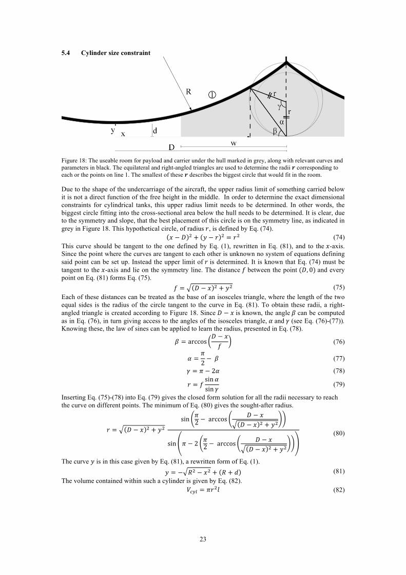
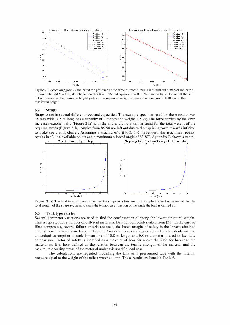
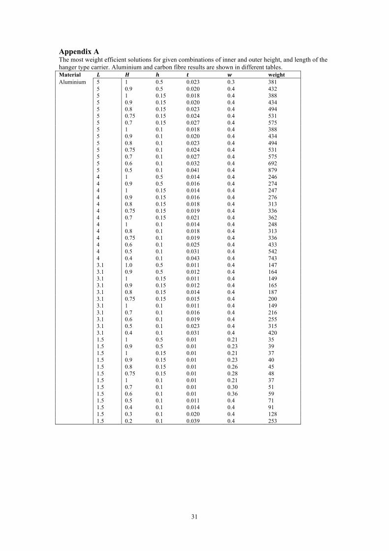
6 Results 6.1 Hanger type load carrier Using optimization (MATLAB function fmincon) with the expressions for the deflections and stresses occurring in the structure as the non-linear boundary conditions, the parameters 𝐻, ℎ, 𝑤, and 𝑡 are chosen for the most weight efficient design of the hanger-type load carrier with cross-section A. The optimization is performed for four different lengths 𝐿 ∈ [1.5, 3.1, 4, 5] , two different materials (aluminium, and carbon fibre composite) and used the constrained intervals 0.01 < 𝑡 < 0.05 and 0.1 < 𝑤 < 0.4 for all cases. The interval for 𝐻 is varied with a lower bounds of 0.11 − 0.6 and upper bounds of 0.2 − 1.0. Similarly the interval of ℎ is varied with upper bounds between 0.1 − 0.5 and a constant lower bound of 0.01. This results in a large set solutions showing the minimum weight for different combinations of 𝐻, ℎ and 𝐿 shown in Figure 19. More detailed results are listed in appendix A. The composite is simplified and modelled a pseudo-isotropic substance with the assumed Young’s modulus 𝐸 = 0.5𝐸!𝑣! + 0.5𝐸!𝑣! [31]. A safety factor of 2 is used for all cases. The results indicate that the highest allowed 𝐻 and ℎ are as expected always optimal, but also that 𝐻 has a strong influence on the weight, while ℎ has a weak influence in comparison. 𝑤 is generally chosen as its upper bound except when 𝑡 reached its lower bound.

Figure 19: The weight of the structure plotted against its maximum height, 𝐻, for different lengths of the structure arms, 𝐿. Both aluminium, solid lines, and carbon fibres dotted lines, are represented for comparison. What looks like one line actually consists of three lines close enough to almost superpose each other. The presence of these is indicated by the star- and square shaped markers, or lack thereof. The line without the markers is generally the longest and represent a minimum height, ℎ = 0.1, star shaped markers indicate ℎ = 1.5, and finally squares ℎ = 0.5. The presence of these lines is further shown in Figure 20.

25

Figure 20: Zoom on figure 17 indicated the presence of the three different lines. Lines without a marker indicate a minimum height ℎ = 0.1, star-shaped marker ℎ = 0.15 and squared ℎ = 0.5. Note in the figure to the left that a 0.4 m increase in the minimum height yields the comparable weight savings to an increase of 0.015 m in the maximum height.

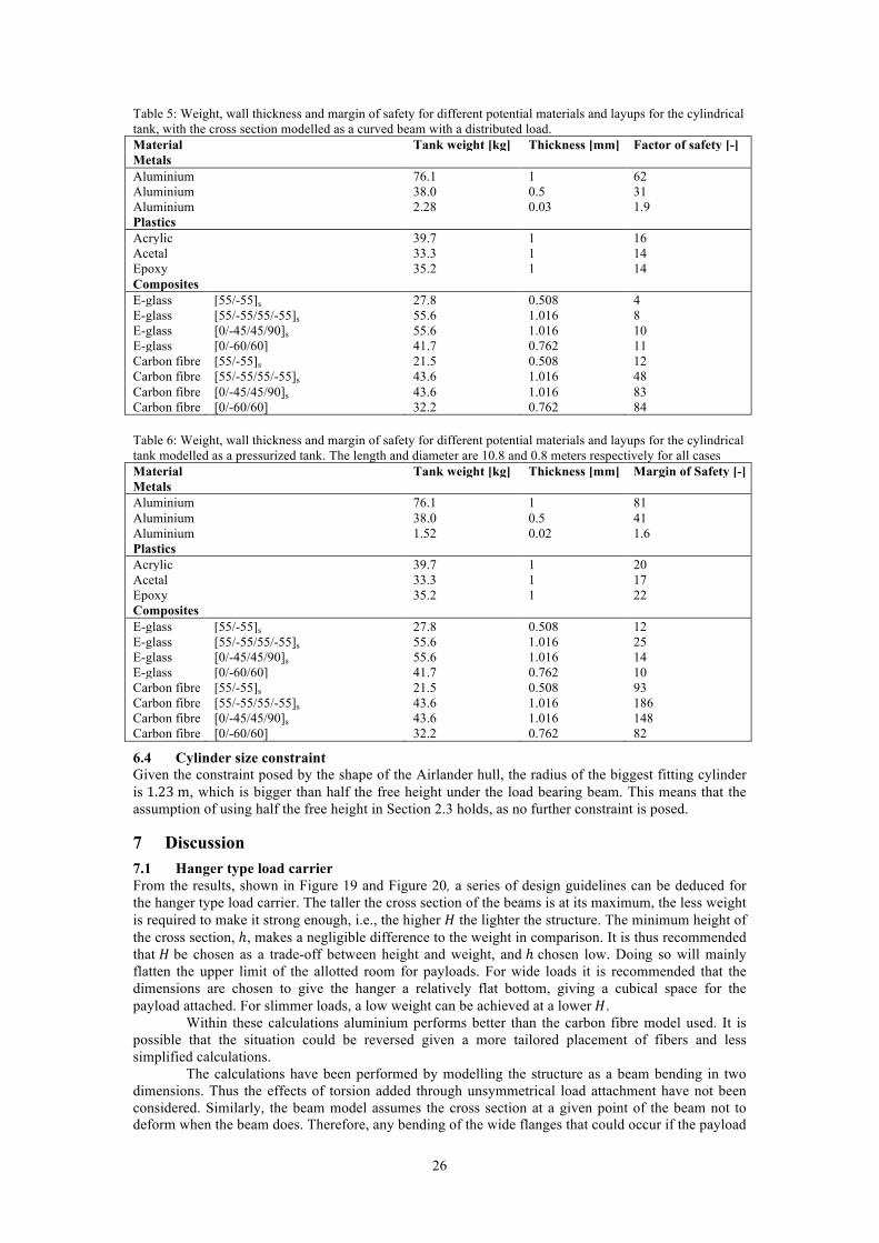
6.2 Straps Straps come in several different sizes and capacities. The example specimen used for these results was 38 mm wide, 4.5 m long, has a capacity of 2 tonnes and weighs 1.5 kg. The force carried by the strap increases exponentially (Figure 21a) with the angle, giving a similar trend for the total weight of the required straps (Figure 21b). Angles from 85-90 are left out due to their quick growth towards infinity, to make the graphs clearer. Assuming a spacing of 𝜕 ∈ [0.3, 1. 0] m between the attachment points, results in 43-146 available points and a maximum allowed angle of 83-87˚. Appendix B shows a zoom.

Figure 21: a) The total tension force carried by the straps as a function of the angle the load is carried at. b) The total weight of the straps required to carry the tension as a function of the angle the load is carried at.

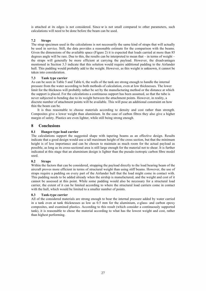
6.3 Tank type carrier Several parameter variations are tried to find the configuration allowing the lowest structural weight. This is repeated for a number of different materials. Data for composites taken from [30]. In the case of fibre composites, several failure criteria are used, the listed margin of safety is the lowest obtained among them.The results are listed in Table 5. Any axial forces are neglected in the first calculation and a standard assumption of tank dimensions of 10.8 m length and 0.8 m diameter is used to facilitate comparison. Factor of safety is included as a measure of how far above the limit for breakage the material is. It is here defined as the relation between the tensile strength of the material and the maximum occuring stress of the material under this specific load case. The calculations are repeated modelling the tank as a pressurized tube with the internal pressure equal to the weight of the tallest water column. These results are listed in Table 6.

26

Table 5: Weight, wall thickness and margin of safety for different potential materials and layups for the cylindrical tank, with the cross section modelled as a curved beam with a distributed load. Material Tank weight [kg] Thickness [mm] Factor of safety [-] Metals Aluminium 76.1 1 62 Aluminium 38.0 0.5 31 Aluminium 2.28 0.03 1.9 Plastics Acrylic 39.7 1 16 Acetal 33.3 1 14 Epoxy 35.2 1 14 Composites E-glass [55/-55]s 27.8 0.508 4 E-glass [55/-55/55/-55]s 55.6 1.016 8 E-glass [0/-45/45/90]s 55.6 1.016 10 E-glass [0/-60/60] 41.7 0.762 11 Carbon fibre [55/-55]s 21.5 0.508 12 Carbon fibre [55/-55/55/-55]s 43.6 1.016 48 Carbon fibre [0/-45/45/90]s 43.6 1.016 83 Carbon fibre [0/-60/60] 32.2 0.762 84 Table 6: Weight, wall thickness and margin of safety for different potential materials and layups for the cylindrical tank modelled as a pressurized tank. The length and diameter are 10.8 and 0.8 meters respectively for all cases Material Tank weight [kg] Thickness [mm] Margin of Safety [-] Metals Aluminium 76.1 1 81 Aluminium 38.0 0.5 41 Aluminium 1.52 0.02 1.6 Plastics Acrylic 39.7 1 20 Acetal 33.3 1 17 Epoxy 35.2 1 22 Composites E-glass [55/-55]s 27.8 0.508 12 E-glass [55/-55/55/-55]s 55.6 1.016 25 E-glass [0/-45/45/90]s 55.6 1.016 14 E-glass [0/-60/60] 41.7 0.762 10 Carbon fibre [55/-55]s 21.5 0.508 93 Carbon fibre [55/-55/55/-55]s 43.6 1.016 186 Carbon fibre [0/-45/45/90]s 43.6 1.016 148 Carbon fibre [0/-60/60] 32.2 0.762 82

6.4 Cylinder size constraint Given the constraint posed by the shape of the Airlander hull, the radius of the biggest fitting cylinder is 1.23 m, which is bigger than half the free height under the load bearing beam. This means that the assumption of using half the free height in Section 2.3 holds, as no further constraint is posed.

7 Discussion 7.1 Hanger type load carrier From the results, shown in Figure 19 and Figure 20, a series of design guidelines can be deduced for the hanger type load carrier. The taller the cross section of the beams is at its maximum, the less weight is required to make it strong enough, i.e., the higher 𝐻 the lighter the structure. The minimum height of the cross section, ℎ, makes a negligible difference to the weight in comparison. It is thus recommended that 𝐻 be chosen as a trade-off between height and weight, and ℎ chosen low. Doing so will mainly flatten the upper limit of the allotted room for payloads. For wide loads it is recommended that the dimensions are chosen to give the hanger a relatively flat bottom, giving a cubical space for the payload attached. For slimmer loads, a low weight can be achieved at a lower 𝐻. Within these calculations aluminium performs better than the carbon fibre model used. It is possible that the situation could be reversed given a more tailored placement of fibers and less simplified calculations. The calculations have been performed by modelling the structure as a beam bending in two dimensions. Thus the effects of torsion added through unsymmetrical load attachment have not been considered. Similarly, the beam model assumes the cross section at a given point of the beam not to deform when the beam does. Therefore, any bending of the wide flanges that could occur if the payload

27

is attached at its edges is not considered. Since 𝑤 is not small compared to other parameters, such calculations will need to be done before the beam can be used.

7.2 Straps The strap specimen used in the calculations is not necessarily the same kind of straps that will actually be used in service. Still, the data provides a reasonable estimate for the comparison with the beams. Given the dimensions of the available space (Figure 2) it is expected that loads carried at more than 85 degrees angle will be rare. Due to this, the results can be interpreted to mean that – in terms of weight – the straps will generally be more efficient at carrying the payload. However, the disadvantages mentioned in Section 3.3 indicate that this solution would require additional padding to the Airlander hull. This padding would probably add to the weight. However, as this weight is unknown, it cannot be taken into consideration.

7.3 Tank type carrier As can be seen in Table 5 and Table 6, the walls of the tank are strong enough to handle the internal pressure from the water according to both methods of calculation, even at low thicknesses. The lower limit for the thickness will probably rather be set by the manufacturing method or the distance at which the support is placed. For the calculations a continuous support has been assumed, so that the tube is never subjected to bending due to its weight between the attachment points. However, in reality, a discrete number of attachment points will be available. This will pose an additional constraint on how thin the beam can be.

It is thus reasonable to choose materials according to density and cost rather than strength. Composites give a lower weight than aluminium. In the case of carbon fibres they also give a higher margin of safety. Plastics are even lighter, while still being strong enough.

8 Conclusions 8.1 Hanger-type load carrier The calculations support the suggested shape with tapering beams as an effective design. Results indicate that a good design would use a tall maximum height of the cross section, but that the minimum height is of less importance and can be chosen to maintain as much room for the actual payload as possible, as long as its cross-sectional area is still large enough for the material not to shear. It is further indicated at this stage that an aluminium design is lighter than the pseudo-isotropic carbon fibre model used.

8.2 Straps Within the factors that can be considered, strapping the payload directly to the load bearing beam of the aircraft proves more efficient in terms of structural weight than using stiff beams. However, the use of straps require a padding on every part of the Airlander hull that the load might come in contact with. This padding needs to be added already when the airship is manufactured, and the weight and cost of it cannot be assessed at this point. While some padding would also be necessary for a structural load carrier, the extent of it can be limited according to where the structural load carriers come in contact with the hull, which would be limited to a smaller number of points.

8.3 Tank-type carrier All of the considered materials are strong enough to bear the internal pressure added by water carried in a tank even at tank thicknesses as low as 0.5 mm for the aluminium, e-glass- and carbon epoxy composites, and examined plastics. According to this result (which consider a continuously supported tank), it is reasonable to chose the material according to what has the lowest weight and cost, rather than highest performing.

28

9 Suggested further work 9.1 Development of the load carrier Further load cases will need to be considered for all of the load carriers, along with more detailed structural analyses when the detailing of the design is done. In addition, since payloads will hang below the airship, the continued structural integrity of the payload needs to be confirmed. It is not sufficient that the carrier is able to carry the load; the load needs be able to carry its own weight without breaking when resting on the attachment points.

9.2 Specializing to specific loads The major part of this work took place before the first flight of the Airlander 10 prototype, which was still undergoing flight certification. The uncertainty of what the market will look like was therefore combated through an assessment of which loads could be realistic. The results of this assessment was the basis for the design. This design is intended to be versatile, to best equip the aircraft for as wide a range of applications as possible. In the future, when the market is better known, there is room for further development. Frequently reoccurring applications might benefit from more specialized modules that could be added to the load carrying system.

9.3 Adapting the solution to other hybrid airships Other similar HAs are expected to enter the market further on. Lockheed Martin and RosAeroSystems are releasing their versions, P-791 and ATLANT 30/100, and HAV is planning a bigger version of Airlander capable of carrying 60 tonnes, Airlander 50. While the principles of flight are similar, the problematics around attaching payload to them changes. The main similarity is the very constrained room the load needs to be carried within, to allow the airship to land. Both P-791 and Airlander 50 have a hull consisting of 3 balloons, thus probably allowing for attachment along two lines, instead of one. ATLANT has a shape maintained by a rigid structure, fundamentally changing the conditions for where, and how much, load can be attached.

9.4 Specific applications It was requested by Ocean Sky that the load carrier be able to work as a water bomber for forest fires. While the problem of carrying water has been addressed, and the specifics for a water bomber not being more farfetched than to add openings to release the water with, there are some expected problems that would need research before it is meaningful to further develop this. As shown in Section 2.3 the hull material is heat sensitive. Further, it is unknown how the air currents due to these fires would affect the HA control. An analysis of the heat and air flow above typical forest fires would thus need to be performed to further explore this feasibility.

29

References [1] AALCO, Aluminium Alloy – Commercial Alloy – 6082 – T6~T651 Plate, data sheet, http://www.aalco.co.uk/datasheets/Aluminium-Alloy-6082-T6T651-Plate_148.ashx accessed 2016-08-18 21:47

[2] AUTODESK, Autodesk helios composite – new item module, picture, https://knowledge.autodesk.com/support/helius-composite/learn-explore/caas/CloudHelp/cloudhelp/2015/ENU/ACMPDS/files/GUID-B36590E7-800A-4B1E-9968-1396B3762773-htm.html accessed 2016-08-19 12:10

[3] BORESI, A.P. et al, Advanced Mechanics of Materials 5th Ed, John Wiley & Sons Inc., USA, 9, pp 362-370

[4] CASSELS, J.W.S., An introduction to Diophantine approximation, Cambridge, Great Britain, 45, (1957)

[5] CORTLAND COMPANY, Vectran 12 Strand & 12x12, Techsheet, http://www.cortlandcompany.com/sites/default/files/downloads/media/product-data-sheets-vectran-12-strand.pdf accessed 2016-06-21 18:30

[6] DUPONT TEIJIN FILMS, Mylar polyester film, Product information, http://usa.dupontteijinfilms.com/informationcenter/downloads/Physical_And_Thermal_Properties.pdf accessed 2016-06-21 18:35

[7] FARNHAM, A., Tumbling Oil Prices Have Given Birth to Two Massive, Dueling Blimps , Fortune, http://fortune.com/2016/04/04/tumbling-oil-prices-have-given-birth-to-two-massive-dueling-blimps/ accessed 2016-06-17 12:31

[8] HAMAK, J. E., Helium, U.S. Geological Survey, Mineral Commodity Summaries, January 2015, http://minerals.usgs.gov/minerals/pubs/commodity/helium/mcs-2015-heliu.pdf accessed 2016-06-17 12:00

[9] HYBRID AIR VEHICLES 2016, Airlander 10, http://www.hybridairvehicles.com/aircraft/airlander-10, accessed 2016-03-23 15:20

[10] HYBRID AIR VEHICLES 2015, Airlander 10 Technical Data, http://www.hybridairvehicles.com/downloads/Airlander-21.pdf, accessed 2015-09-23 13:00

[11] HYBRID AIR VEHICLES 2015, Airlander assembly complete – on time and on budget, http://www.hybridairvehicles.com/news-and-media/news/airlander-assembly-complete-on-time-and-on-budget

[12] HYBRID AIR VEHICLES 2016, http://www.hybridairvehicles.com/, accessed 2016-03-31 17:15

[13] IATA, Fuel Price Analysis, http://www.iata.org/publications/economics/fuel-monitor/Pages/price-analysis.aspx, accessed 2016-06-20 15:40

[14] KURARAY, Vectran Thermal Properties, http://www.vectranfiber.com/properties/thermal-properties/ accessed 2016-06-21 18:30

[15] LOCKHEED MARTIN 2016, P-791, http://lockheedmartin.com/us/products/HybridAirship.html, accessed 2016-03-31 17:16

[16] LUNDH., H., Hållfasthetslära, KTH, Stockholm, 9, pp 180-181, (2007)

[17] LÖNESTATISTIK.SE, Pilot, http://www.lonestatistik.se/loner.asp/yrke/Pilot-1153, accessed 2016-06-17 12:11

30

[18] MEGSON, T.H.G., Aircraft Structures for Engineering Students 5th Ed., Elsevier, United Kingdom, 1, 16, pp 5-8, 492-499

[19] MILBERG, E., Airlander 10, World’s Largest Aircraft, Gets of the Ground, ACMA Composites Manufacturing Magazine, March 2016

[20] MILLER, W. M. JR., The Dynairship, Proceedings of the Interagency Workshop on Lighter than Air Vehicles, MIT Flight Transportation Laboratory, Cambridge, pp. 443, January 1975

[21] PROFESSIONAL PLASTICS, Typical properties of Acetals, data sheet, http://www.professionalplastics.com/professionalplastics/content/Acetal_Delrin.pdf, accessed 2016-08-17 14:16

[22] PROFESSIONAL PLASTICS, Typical properties of Acrylics, data sheet, http://www.professionalplastics.com/professionalplastics/content/Acetal_Delrin.pdf, accessed 2016-08-17 14:16

[23] RICE UNIVERSITY MECH 400, Bending of Curved Beams – Strength of Materials Approach, https://www.clear.rice.edu/mech400/Winkler_curved_beam_theory.pdf, accessed 2016-08-10 10:59

[24] ROSAEROSYSTEMS 2016, ATLANT, http://rosaerosystems.com/atlant/, accessed 2016-03-31 17:16

[25] SUNDSTRÖM, B., Handbok och formelsamling i Hållfasthetslära 7th Ed., Instutionen för hållfasthetslära KTH, Stockholm, 3, pp 26-27

[26] TORENBEEK, E., WITTENBERG, H., Flight Physics, Springer, Delft, Netherlands , 2, pp 49-51, (2009)

[27] TIMOSCHENKO S., GOODIER, J.N., Theory of elasticity, McGraw-Hill Book Company Inc., (1951)

[28] WELCH FLUOROCARBON INC., PVF, Polybvinyl fluoride, http://www.welchfluorocarbon.com/material-profiles/films/pvf/ accessed 2016-06-21 18:37

[29] WINDPOWER MONTHLY, Staying ahead of transport challenges, www.windpowermonthly.com/article/1187598/staying-ahead-transport-challanges, July 01 (2013), accessed 2016-08-04 14:45

[30] ZENKERT, D., BATTLEY, M., , Foundations of Fibre Composites, KTH, 3, 4, pp 3.12-14, 3.22-23, 3.27, 4.5, 4.9-12, 4.15-16 (2013)

[31] ÅSTRÖM, B.T., Manufacturing of Polymer Composites, Nelson Thornes Ltd, Cheltenham, UK, 3, pp 143, 152, (2002)

31

Appendix A The most weight efficient solutions for given combinations of inner and outer height, and length of the hanger type carrier. Aluminium and carbon fibre results are shown in different tables. Material 𝑳 𝑯 𝒉 𝒕 𝒘 weight Aluminium 5 1 0.5 0.023 0.3 381 5 0.9 0.5 0.020 0.4 432 5 1 0.15 0.018 0.4 388 5 0.9 0.15 0.020 0.4 434 5 0.8 0.15 0.023 0.4 494 5 0.75 0.15 0.024 0.4 531 5 0.7 0.15 0.027 0.4 575 5 1 0.1 0.018 0.4 388 5 0.9 0.1 0.020 0.4 434 5 0.8 0.1 0.023 0.4 494 5 0.75 0.1 0.024 0.4 531 5 0.7 0.1 0.027 0.4 575 5 0.6 0.1 0.032 0.4 692 5 0.5 0.1 0.041 0.4 879 4 1 0.5 0.014 0.4 246 4 0.9 0.5 0.016 0.4 274 4 1 0.15 0.014 0.4 247 4 0.9 0.15 0.016 0.4 276 4 0.8 0.15 0.018 0.4 313 4 0.75 0.15 0.019 0.4 336 4 0.7 0.15 0.021 0.4 362 4 1 0.1 0.014 0.4 248 4 0.8 0.1 0.018 0.4 313 4 0.75 0.1 0.019 0.4 336 4 0.6 0.1 0.025 0.4 433 4 0.5 0.1 0.031 0.4 542 4 0.4 0.1 0.043 0.4 743 3.1 1.0 0.5 0.011 0.4 147 3.1 0.9 0.5 0.012 0.4 164 3.1 1 0.15 0.011 0.4 149 3.1 0.9 0.15 0.012 0.4 165 3.1 0.8 0.15 0.014 0.4 187 3.1 0.75 0.15 0.015 0.4 200 3.1 1 0.1 0.011 0.4 149 3.1 0.7 0.1 0.016 0.4 216 3.1 0.6 0.1 0.019 0.4 255 3.1 0.5 0.1 0.023 0.4 315 3.1 0.4 0.1 0.031 0.4 420 1.5 1 0.5 0.01 0.21 35 1.5 0.9 0.5 0.01 0.23 39 1.5 1 0.15 0.01 0.21 37 1.5 0.9 0.15 0.01 0.23 40 1.5 0.8 0.15 0.01 0.26 45 1.5 0.75 0.15 0.01 0.28 48 1.5 1 0.1 0.01 0.21 37 1.5 0.7 0.1 0.01 0.30 51 1.5 0.6 0.1 0.01 0.36 59 1.5 0.5 0.1 0.011 0.4 71 1.5 0.4 0.1 0.014 0.4 91 1.5 0.3 0.1 0.020 0.4 128 1.5 0.2 0.1 0.039 0.4 253

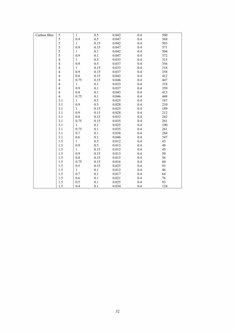
32

Carbon fibre 5 1 0.5 0.042 0.4 500 5 0.9 0.5 0.047 0.4 569 5 1 0.15 0.042 0.4 503 5 0.9 0.15 0.047 0.4 571 5 1 0.1 0.042 0.4 504 5 0.9 0.1 0.047 0.4 572 4 1 0.5 0.033 0.4 315 4 0.9 0.5 0.037 0.4 356 4 1 0.15 0.033 0.4 318 4 0.9 0.15 0.037 0.4 358 4 0.8 0.15 0.043 0.4 412 4 0.75 0.15 0.046 0.4 447 4 1 0.1 0.033 0.4 318 4 0.9 0.1 0.037 0.4 359 4 0.8 0.1 0.043 0.4 413 4 0.75 0.1 0.046 0.4 448 3.1 1 0.5 0.025 0.4 187 3.1 0.9 0.5 0.028 0.4 210 3.1 1 0.15 0.025 0.4 189 3.1 0.9 0.15 0.028 0.4 212 3.1 0.8 0.15 0.032 0.4 242 3.1 0.75 0.15 0.035 0.4 261 3.1 1 0.1 0.025 0.4 190 3.1 0.75 0.1 0.035 0.4 261 3.1 0.7 0.1 0.038 0.4 284 3.1 0.6 0.1 0.046 0.4 347 1.5 1 0.5 0.012 0.4 43 1.5 0.9 0.5 0.013 0.4 48 1.5 1 0.15 0.012 0.4 45 1.5 0.9 0.15 0.013 0.4 50 1.5 0.8 0.15 0.015 0.4 56 1.5 0.75 0.15 0.016 0.4 60 1.5 0.5 0.15 0.025 0.4 93 1.5 1 0.1 0.012 0.4 46 1.5 0.7 0.1 0.017 0.4 64 1.5 0.6 0.1 0.021 0.4 76 1.5 0.5 0.1 0.025 0.4 93 1.5 0.4 0.1 0.034 0.4 124

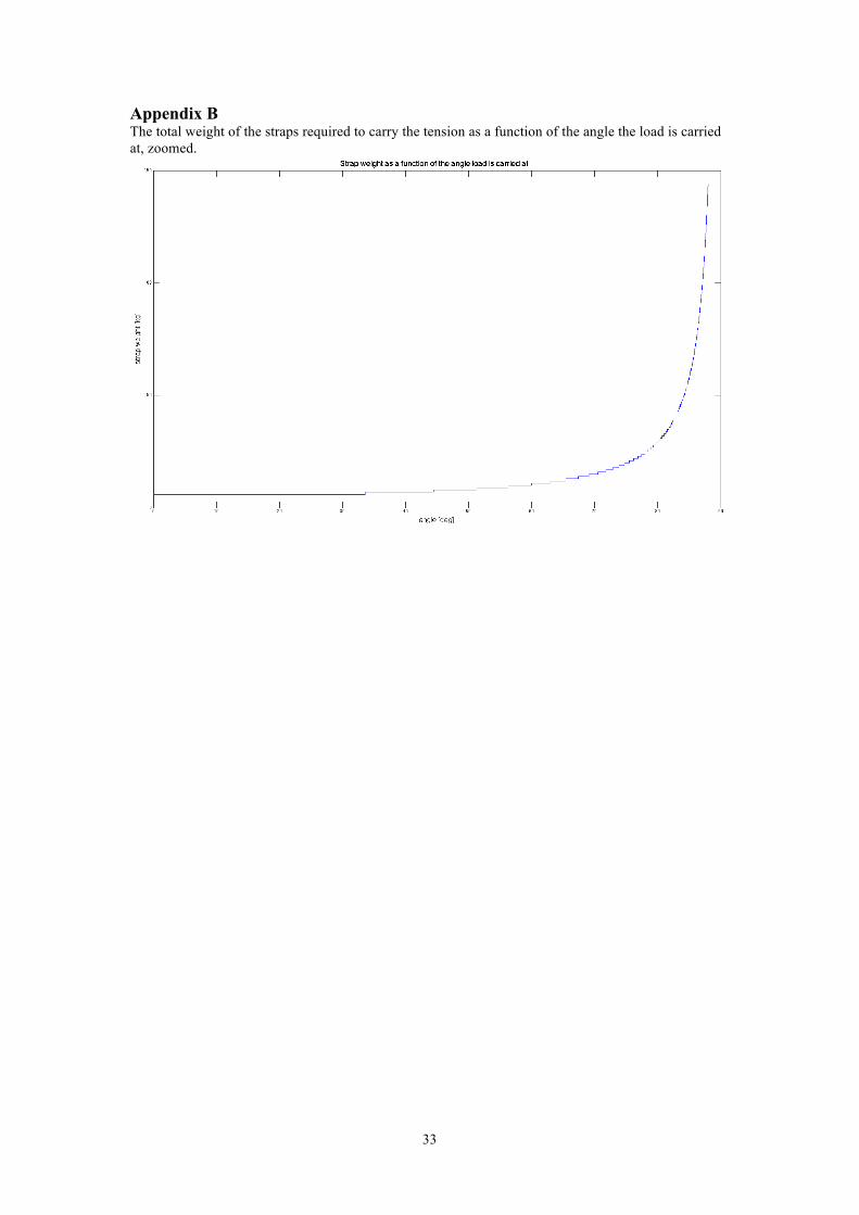
33

Appendix B The total weight of the straps required to carry the tension as a function of the angle the load is carried at, zoomed.

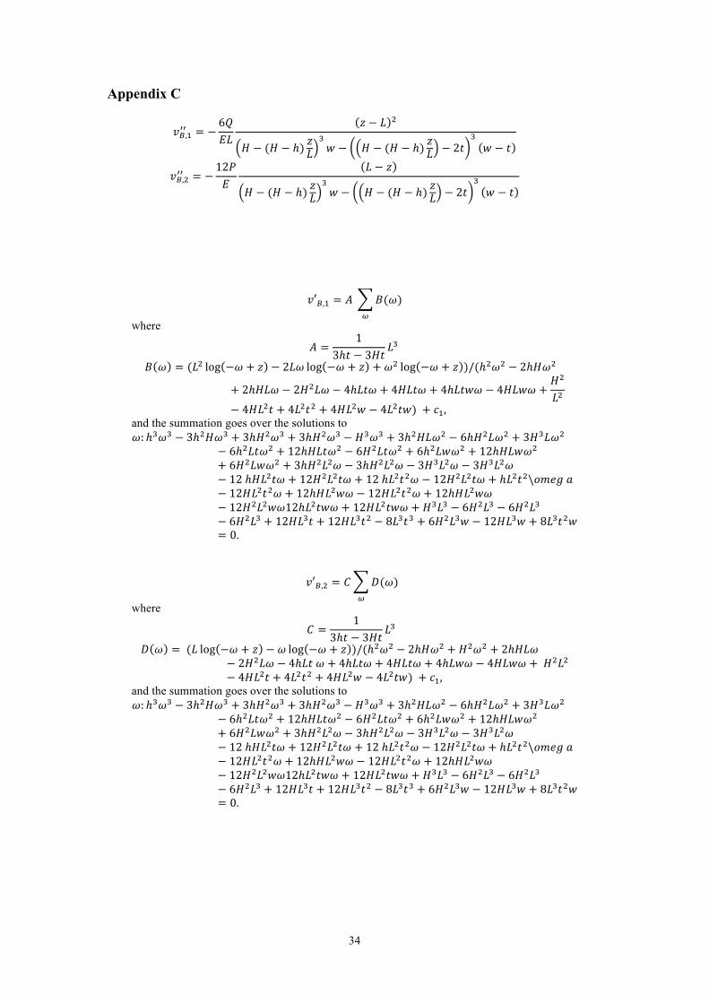
34

Appendix C

𝑣!,!!! = −6𝑄𝐸𝐿

𝑧 − 𝐿 !

𝐻 − (𝐻 − ℎ) 𝑧𝐿!𝑤 − 𝐻 − (𝐻 − ℎ) 𝑧𝐿 − 2𝑡

!𝑤 − 𝑡

𝑣!,!!! = −12𝑃𝐸

𝐿 − 𝑧

𝐻 − (𝐻 − ℎ) 𝑧𝐿!𝑤 − 𝐻 − (𝐻 − ℎ) 𝑧𝐿 − 2𝑡

!𝑤 − 𝑡

𝑣′!,! = 𝐴 𝐵(𝜔)

!

where

𝐴 =1

3ℎ𝑡 − 3𝐻𝑡𝐿!

𝐵 𝜔 = (𝐿! log −𝜔 + 𝑧 − 2𝐿𝜔 log −𝜔 + 𝑧 + 𝜔! log −𝜔 + 𝑧 )/(ℎ!𝜔! − 2ℎ𝐻𝜔!

+ 2ℎ𝐻𝐿𝜔 − 2𝐻!𝐿𝜔 − 4ℎ𝐿𝑡𝜔 + 4𝐻𝐿𝑡𝜔 + 4ℎ𝐿𝑡𝑤𝜔 − 4𝐻𝐿𝑤𝜔 +𝐻!

𝐿!− 4𝐻𝐿!𝑡 + 4𝐿!𝑡! + 4𝐻𝐿!𝑤 − 4𝐿!𝑡𝑤) + 𝑐!,

and the summation goes over the solutions to 𝜔: ℎ!𝜔! − 3ℎ!𝐻𝜔! + 3ℎ𝐻!𝜔! + 3ℎ𝐻!𝜔! − 𝐻!𝜔! + 3ℎ!𝐻𝐿𝜔! − 6ℎ𝐻!𝐿𝜔! + 3𝐻!𝐿𝜔!

− 6ℎ!𝐿𝑡𝜔! + 12ℎ𝐻𝐿𝑡𝜔! − 6𝐻!𝐿𝑡𝜔! + 6ℎ!𝐿𝑤𝜔! + 12ℎ𝐻𝐿𝑤𝜔!

+ 6𝐻!𝐿𝑤𝜔! + 3ℎ𝐻!𝐿!𝜔 − 3ℎ𝐻!𝐿!𝜔 − 3𝐻!𝐿!𝜔 − 3𝐻!𝐿!𝜔− 12 ℎ𝐻𝐿!𝑡𝜔 + 12𝐻!𝐿!𝑡𝜔 + 12 ℎ𝐿!𝑡!𝜔 − 12𝐻!𝐿!𝑡𝜔 + ℎ𝐿!𝑡!\𝑜𝑚𝑒𝑔 𝑎− 12𝐻𝐿!𝑡!𝜔 + 12ℎ𝐻𝐿!𝑤𝜔 − 12𝐻𝐿!𝑡!𝜔 + 12ℎ𝐻𝐿!𝑤𝜔− 12𝐻!𝐿!𝑤𝜔12ℎ𝐿!𝑡𝑤𝜔 + 12𝐻𝐿!𝑡𝑤𝜔 + 𝐻!𝐿! − 6𝐻!𝐿! − 6𝐻!𝐿!− 6𝐻!𝐿! + 12𝐻𝐿!𝑡 + 12𝐻𝐿!𝑡! − 8𝐿!𝑡! + 6𝐻!𝐿!𝑤 − 12𝐻𝐿!𝑤 + 8𝐿!𝑡!𝑤= 0.

𝑣′!,! = 𝐶 𝐷(𝜔) !

where

𝐶 =1

3ℎ𝑡 − 3𝐻𝑡𝐿!

𝐷 𝜔 = (𝐿 log −𝜔 + 𝑧 − 𝜔 log −𝜔 + 𝑧 )/(ℎ!𝜔! − 2ℎ𝐻𝜔! + 𝐻!𝜔! + 2ℎ𝐻𝐿𝜔− 2𝐻!𝐿𝜔 − 4ℎ𝐿𝑡 𝜔 + 4ℎ𝐿𝑡𝜔 + 4𝐻𝐿𝑡𝜔 + 4ℎ𝐿𝑤𝜔 − 4𝐻𝐿𝑤𝜔 + 𝐻!𝐿!− 4𝐻𝐿!𝑡 + 4𝐿!𝑡! + 4𝐻𝐿!𝑤 − 4𝐿!𝑡𝑤) + 𝑐!,

and the summation goes over the solutions to 𝜔: ℎ!𝜔! − 3ℎ!𝐻𝜔! + 3ℎ𝐻!𝜔! + 3ℎ𝐻!𝜔! − 𝐻!𝜔! + 3ℎ!𝐻𝐿𝜔! − 6ℎ𝐻!𝐿𝜔! + 3𝐻!𝐿𝜔!

− 6ℎ!𝐿𝑡𝜔! + 12ℎ𝐻𝐿𝑡𝜔! − 6𝐻!𝐿𝑡𝜔! + 6ℎ!𝐿𝑤𝜔! + 12ℎ𝐻𝐿𝑤𝜔!

+ 6𝐻!𝐿𝑤𝜔! + 3ℎ𝐻!𝐿!𝜔 − 3ℎ𝐻!𝐿!𝜔 − 3𝐻!𝐿!𝜔 − 3𝐻!𝐿!𝜔− 12 ℎ𝐻𝐿!𝑡𝜔 + 12𝐻!𝐿!𝑡𝜔 + 12 ℎ𝐿!𝑡!𝜔 − 12𝐻!𝐿!𝑡𝜔 + ℎ𝐿!𝑡!\𝑜𝑚𝑒𝑔 𝑎− 12𝐻𝐿!𝑡!𝜔 + 12ℎ𝐻𝐿!𝑤𝜔 − 12𝐻𝐿!𝑡!𝜔 + 12ℎ𝐻𝐿!𝑤𝜔− 12𝐻!𝐿!𝑤𝜔12ℎ𝐿!𝑡𝑤𝜔 + 12𝐻𝐿!𝑡𝑤𝜔 + 𝐻!𝐿! − 6𝐻!𝐿! − 6𝐻!𝐿!− 6𝐻!𝐿! + 12𝐻𝐿!𝑡 + 12𝐻𝐿!𝑡! − 8𝐿!𝑡! + 6𝐻!𝐿!𝑤 − 12𝐻𝐿!𝑤 + 8𝐿!𝑡!𝑤= 0.

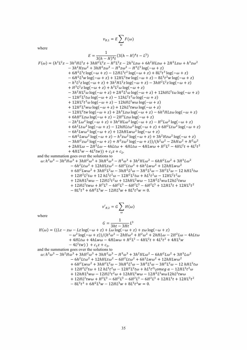
35

𝑣!,! = 𝐸 𝐹(𝜔) !

where

𝐸 =1

3 ℎ − 𝐻 !𝑡3 ℎ − 𝐻 !𝑡 − 𝐿!

𝐹 𝜔 = ℎ!𝐿!𝑧 − 3ℎ!𝐻𝐿!𝑧 + 3ℎ𝐻!𝐿!𝑧 − 𝐻!𝐿!𝑧 − 2ℎ!𝐿𝑧𝜔 + 6ℎ!𝐻𝐿𝑧𝜔 + 2𝐻!𝐿𝑧𝜔 + ℎ!𝑧𝜔!

− 3ℎ!𝐻𝑧𝜔! + 3ℎ𝐻!𝑧𝜔! − 𝐻!𝑧𝜔! − 𝐻!𝐿! log −𝜔 + 𝑧+ 6𝐻!𝐿!𝑡 log −𝜔 + 𝑧 − 12𝐻𝐿!𝑡! log −𝜔 + 𝑧 + 8𝐿!𝑡! log −𝜔 + 𝑧− 6𝐻!𝐿!𝑤 log −𝜔 + 𝑧 + 12𝐻𝐿!𝑡𝑤 log −𝜔 + 𝑧 − 8𝐿!𝑡!𝑤 log −𝜔 + 𝑧− ℎ!𝐿!𝑧 log −𝜔 + 𝑧 + 3ℎ!𝐻𝐿!𝑧 log −𝜔 + 𝑧 − 3ℎ𝐻!𝐿!𝑧 log −𝜔 + 𝑧+ 𝐻!𝐿!𝑧 log −𝜔 + 𝑧 + ℎ!𝐿!𝜔 log −𝜔 + 𝑧− 3ℎ!𝐻𝐿!𝜔 log −𝜔 + 𝑧 + 2𝐻!𝐿!𝜔 log −𝜔 + 𝑧 + 12ℎ𝐻𝐿!𝑡𝜔 log −𝜔 + 𝑧− 12𝐻!𝐿!𝑡𝜔 log −𝜔 + 𝑧 − 12ℎ𝐿!𝑡!𝜔 log −𝜔 + 𝑧+ 12𝐻𝐿!𝑡!𝜔 log −𝜔 + 𝑧 − 12ℎ𝐻𝐿!𝑤𝜔 log −𝜔 + 𝑧+ 12𝐻!𝐿!𝑤𝜔 log −𝜔 + 𝑧 + 12ℎ𝐿!𝑡𝑤𝜔 log −𝜔 + 𝑧− 12𝐻𝐿!𝑡𝑤 log −𝜔 + 𝑧 + 2ℎ!𝐿𝑧𝜔 log −𝜔 + 𝑧 − 6ℎ!𝐻𝐿𝑧𝜔 log −𝜔 + 𝑧+ 6ℎ𝐻!𝐿𝑧𝜔 log −𝜔 + 𝑧 − 2𝐻!𝐿𝑧𝜔 log −𝜔 + 𝑧− 2ℎ!𝐿𝜔! log −𝜔 + 𝑧 + 3ℎ!𝐻𝐿𝜔! log −𝜔 + 𝑧 − 𝐻!𝐿𝜔! log −𝜔 + 𝑧+ 6ℎ!𝐿𝑡𝜔! log −𝜔 + 𝑧 − 12ℎ𝐻𝐿𝑡𝜔! log −𝜔 + 𝑧 + 6𝐻!𝐿𝑡𝜔! log −𝜔 + 𝑧− 6ℎ!𝐿𝑤𝜔! log −𝜔 + 𝑧 + 12ℎ𝐻𝐿𝑤𝜔! log −𝜔 + 𝑧− 6𝐻!𝐿𝑤𝜔! log −𝜔 + 𝑧 − ℎ!𝑧𝜔! log −𝜔 + 𝑧 + 3ℎ!𝐻𝑧𝜔! log −𝜔 + 𝑧− 3ℎ𝐻!𝑧𝜔! log −𝜔 + 𝑧 + 𝐻!𝑧𝜔! log −𝜔 + 𝑧 /(ℎ!𝜔! − 2ℎ𝐻𝜔! + 𝐻!𝜔!

+ 2ℎ𝐻𝐿𝜔 − 2𝐻!𝐿𝜔 − 4ℎ𝐿𝑡𝜔 + 4𝐻𝐿𝑡𝜔 − 4𝐻𝐿𝑤𝜔 + 𝐻!𝐿! − 4𝐻𝐿!𝑡 + 4𝐿!𝑡!+ 4𝐻𝐿!𝑤 − 4𝐿!𝑡𝑤)) + 𝑐!𝑧 + 𝑐!,

and the summation goes over the solutions to 𝜔: ℎ!𝜔! − 3ℎ!𝐻𝜔! + 3ℎ𝐻!𝜔! + 3ℎ𝐻!𝜔! − 𝐻!𝜔! + 3ℎ!𝐻𝐿𝜔! − 6ℎ𝐻!𝐿𝜔! + 3𝐻!𝐿𝜔!

− 6ℎ!𝐿𝑡𝜔! + 12ℎ𝐻𝐿𝑡𝜔! − 6𝐻!𝐿𝑡𝜔! + 6ℎ!𝐿𝑤𝜔! + 12ℎ𝐻𝐿𝑤𝜔!

+ 6𝐻!𝐿𝑤𝜔! + 3ℎ𝐻!𝐿!𝜔 − 3ℎ𝐻!𝐿!𝜔 − 3𝐻!𝐿!𝜔 − 3𝐻!𝐿!𝜔 − 12 ℎ𝐻𝐿!𝑡𝜔+ 12𝐻!𝐿!𝑡𝜔 + 12 ℎ𝐿!𝑡!𝜔 − 12𝐻!𝐿!𝑡𝜔 + ℎ𝐿!𝑡!𝜔 − 12𝐻𝐿!𝑡!𝜔+ 12ℎ𝐻𝐿!𝑤𝜔 − 12𝐻𝐿!𝑡!𝜔 + 12ℎ𝐻𝐿!𝑤𝜔 − 12𝐻!𝐿!𝑤𝜔12ℎ𝐿!𝑡𝑤𝜔+ 12𝐻𝐿!𝑡𝑤𝜔 + 𝐻!𝐿! − 6𝐻!𝐿! − 6𝐻!𝐿! − 6𝐻!𝐿! + 12𝐻𝐿!𝑡 + 12𝐻𝐿!𝑡!− 8𝐿!𝑡! + 6𝐻!𝐿!𝑤 − 12𝐻𝐿!𝑤 + 8𝐿!𝑡!𝑤 = 0.

𝑣′!,! = 𝐺 𝐻 𝜔 !

where

𝐺 =1

3ℎ𝑡 − 3𝐻𝑡𝐿!

𝐻 𝜔 = (𝐿𝑧 − 𝑧𝜔 − 𝐿𝑧 log −𝜔 + 𝑧 + 𝐿𝜔 log −𝜔 + 𝑧 + 𝑧𝜔 log −𝜔 + 𝑧− 𝜔! log −𝜔 + 𝑧 )/(ℎ!𝜔! − 2ℎ𝐻𝜔! + 𝐻!𝜔! + 2ℎ𝐻𝐿𝜔 − 2𝐻!𝐿𝜔 − 4ℎ𝐿𝑡𝜔+ 4𝐻𝐿𝑡𝜔 + 4ℎ𝐿𝑤𝜔 − 4𝐻𝐿𝑤𝜔 + 𝐻!𝐿! − 4𝐻𝐿!𝑡 + 4𝐿!𝑡! + 4𝐻𝐿!𝑤− 4𝐿!𝑡𝑤) + 𝑐!𝑧 + 𝑐!,

and the summation goes over the solutions to 𝜔: ℎ!𝜔! − 3ℎ!𝐻𝜔! + 3ℎ𝐻!𝜔! + 3ℎ𝐻!𝜔! − 𝐻!𝜔! + 3ℎ!𝐻𝐿𝜔! − 6ℎ𝐻!𝐿𝜔! + 3𝐻!𝐿𝜔!

− 6ℎ!𝐿𝑡𝜔! + 12ℎ𝐻𝐿𝑡𝜔! − 6𝐻!𝐿𝑡𝜔! + 6ℎ!𝐿𝑤𝜔! + 12ℎ𝐻𝐿𝑤𝜔!

+ 6𝐻!𝐿𝑤𝜔! + 3ℎ𝐻!𝐿!𝜔 − 3ℎ𝐻!𝐿!𝜔 − 3𝐻!𝐿!𝜔 − 3𝐻!𝐿!𝜔 − 12 ℎ𝐻𝐿!𝑡𝜔+ 12𝐻!𝐿!𝑡𝜔 + 12 ℎ𝐿!𝑡!𝜔 − 12𝐻!𝐿!𝑡𝜔 + ℎ𝐿!𝑡!\𝑜𝑚𝑒𝑔 𝑎 − 12𝐻𝐿!𝑡!𝜔+ 12ℎ𝐻𝐿!𝑤𝜔 − 12𝐻𝐿!𝑡!𝜔 + 12ℎ𝐻𝐿!𝑤𝜔 − 12𝐻!𝐿!𝑤𝜔12ℎ𝐿!𝑡𝑤𝜔+ 12𝐻𝐿!𝑡𝑤𝜔 + 𝐻!𝐿! − 6𝐻!𝐿! − 6𝐻!𝐿! − 6𝐻!𝐿! + 12𝐻𝐿!𝑡 + 12𝐻𝐿!𝑡!− 8𝐿!𝑡! + 6𝐻!𝐿!𝑤 − 12𝐻𝐿!𝑤 + 8𝐿!𝑡!𝑤 = 0.

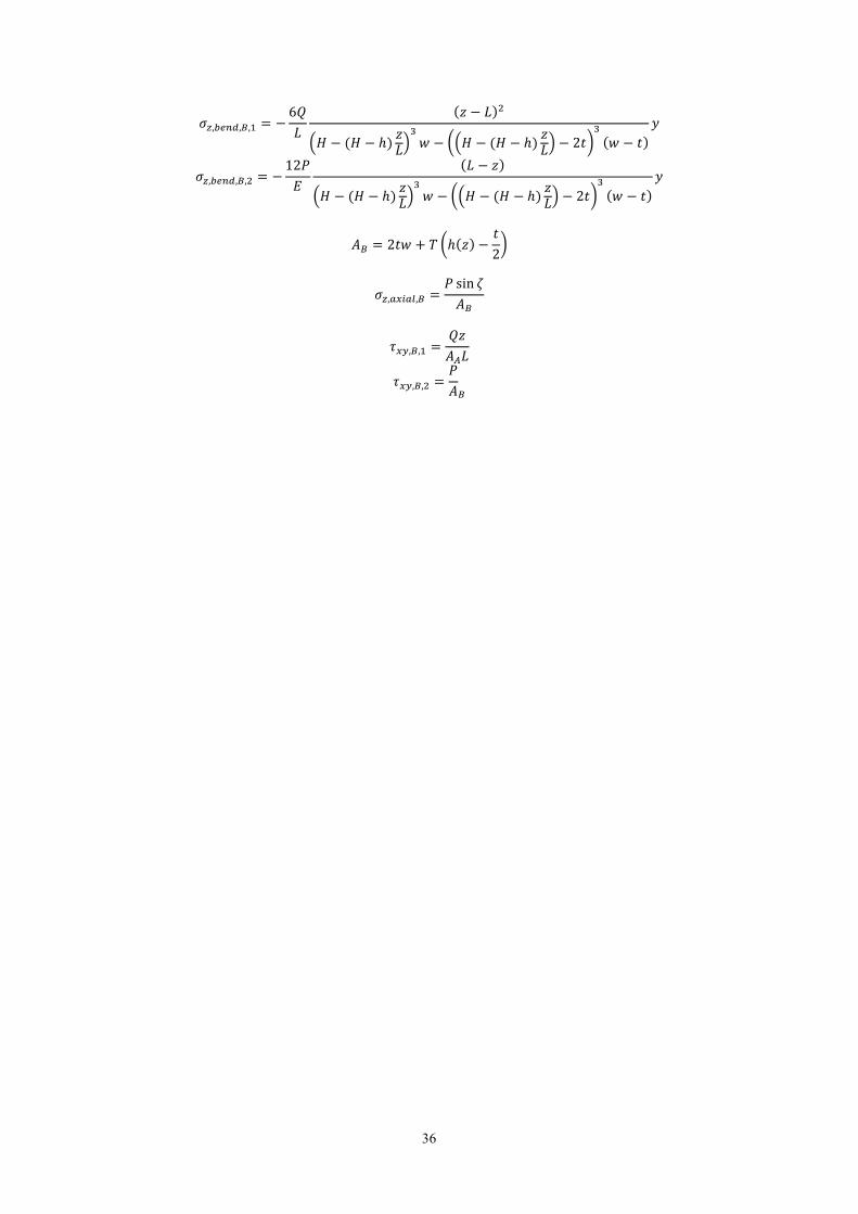
36

𝜎!,!"#$,!,! = −

6𝑄𝐿

𝑧 − 𝐿 !

𝐻 − (𝐻 − ℎ) 𝑧𝐿!𝑤 − 𝐻 − (𝐻 − ℎ) 𝑧𝐿 − 2𝑡

!𝑤 − 𝑡

𝑦

𝜎!,!"#$,!,! = −

12𝑃𝐸

𝐿 − 𝑧

𝐻 − (𝐻 − ℎ) 𝑧𝐿!𝑤 − 𝐻 − (𝐻 − ℎ) 𝑧𝐿 − 2𝑡

!𝑤 − 𝑡

𝑦

𝐴! = 2𝑡𝑤 + 𝑇 ℎ 𝑧 −

𝑡2

𝜎!,!"#!$,! =𝑃 sin 𝜁𝐴!

𝜏!",!,! =𝑄𝑧𝐴!𝐿

𝜏!",!,! =𝑃𝐴!

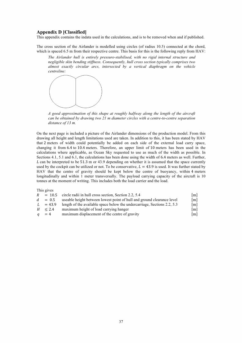
37

Appendix D [Classified] This appendix contains the indata used in the calculations, and is to be removed when and if published. The cross section of the Airlander is modelled using circles (of radius 10.5) connected at the chord, which is spaced 6.5 m from their respective centre. This basis for this is the following reply from HAV:

The Airlander hull is entirely pressure-stabilised, with no rigid internal structure and negligible skin bending stiffness. Consequently, hull cross section typically comprises two almost exactly circular arcs, intersected by a vertical diaphragm on the vehicle centreline:

A good approximation of this shape at roughly halfway along the length of the aircraft can be obtained by drawing two 21 m diameter circles with a centre-to-centre separation distance of 13 m.

On the next page is included a picture of the Airlander dimensions of the production model. From this drawing all height and length limitations used are taken. In addition to this, it has been stated by HAV that 2 meters of width could potentially be added on each side of the external load carry space, changing it from 6.4 to 10.4 meters. Therefore, an upper limit of 10 meters has been used in the calculations where applicable, as Ocean Sky requested to use as much of the width as possible. In Sections 4.1, 5.1 and 6.1, the calculations has been done using the width of 6.4 meters as well. Further, 𝐿 can be interpreted to be 51.3 m or 43.9 depending on whether it is assumed that the space currently used by the cockpit can be utilized or not. To be conservative, 𝐿 = 43.9 is used. It was further stated by HAV that the centre of gravity should be kept below the centre of buoyancy, within 4 meters longitudinally and within 1 meter transversally. The payload carrying capacity of the aircraft is 10 tonnes at the moment of writing. This includes both the load carrier and the load. This gives 𝑅 = 10.5 circle radii in hull cross section, Section 2.2, 5.4 m 𝑑 = 0.5 useable height between lowest point of hull and ground clearance level m 𝐿 = 43.9 length of the available space below the undercarriage, Sections 2.2, 5.3 m 𝐻 ≤ 2.4 maximum height of load carrying hanger m 𝑞 = 4 maximum displacement of the centre of gravity m

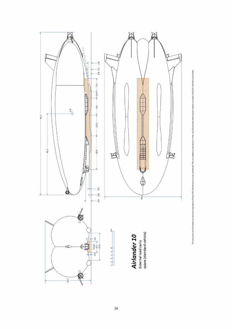
38