Design of Active Magnetic Bearing Controllers for Rotors

General rights Copyright and moral rights for the publications made accessible in the public portal are retained by the authors and/or other copyright owners and it is a condition of accessing publications that users recognise and abide by the legal requirements associated with these rights.

Users may download and print one copy of any publication from the public portal for the purpose of private study or research.

You may not further distribute the material or use it for any profit-making activity or commercial gain

You may freely distribute the URL identifying the publication in the public portal If you believe that this document breaches copyright please contact us providing details, and we will remove access to the work immediately and investigate your claim.

Downloaded from orbit.dtu.dk on: Oct 10, 2021

Design of Active Magnetic Bearing Controllers for Rotors Subjected to Gas SealForces

Lauridsen, Jonas Skjødt; Santos, Ilmar F.

Published in:Journal of Dynamic Systems, Measurement and Control

Link to article, DOI:10.1115/1.4039665

Publication date:2018

Document VersionPeer reviewed version

Link back to DTU Orbit

Citation (APA):Lauridsen, J. S., & Santos, I. F. (2018). Design of Active Magnetic Bearing Controllers for Rotors Subjected toGas Seal Forces. Journal of Dynamic Systems, Measurement and Control, 140(9), [091015 ].https://doi.org/10.1115/1.4039665

https://doi.org/10.1115/1.4039665

https://orbit.dtu.dk/en/publications/ff8fead7-ca71-4ad9-bb2b-b7adf82999df

https://doi.org/10.1115/1.4039665

Design of Active Magnetic Bearing Controllersfor Rotors Subjected to Gas Seal Forces

Jonas S. Lauridsen∗PhD student, Member of ASME

Department of Mechanical EngineeringTechnical University of Denmark

Email: [email protected]

Ilmar F. Santos†

Professor, Member of ASMEDepartment of Mechanical Engineering

Technical University of DenmarkEmail: [email protected]

Proper design of feedback controllers is crucial for ensu-ring high performance of Active Magnetic Bearing (AMB)supported rotor dynamic systems. Annular seals in those sy-stems can contribute significant forces, which, in many cases,are hard to model in advance due to complex geometries ofthe seal and multiphase fluids. Hence, it can be challengingto design AMB controllers that will guarantee robust perfor-mance for these kinds of systems. This paper demonstratesthe design, simulation and experimental results of model ba-sed controllers for AMB systems, subjected to dynamic sealforces. The controllers are found using H∞ and µ synthe-sis and are based on a global rotor dynamic model in-whichthe seal coefficients are identified in-situ. The controllers areimplemented in a rotor-dynamic test facility with two radialAMBs and one annular seal with an adjustable inlet pres-sure. The seal is a smooth annular type, with large clearance(worn seal) and with high pre-swirl, which generates signifi-cant cross-coupled forces. The H∞ controller is designed tocompensate for the seal forces and the µ controller is furt-hermore designed to be robust against a range of pressuresacross the seal. In this study the rotor is non-rotating. Ex-perimental and simulation results show that significant per-formance can be achieved using the model based controllerscompared to a reference decentralised Proportional IntegralDerivative (PID) controller and robustness against large va-riations of pressure across the seal can be improved by useof robust synthesised controllers.

∗Address all correspondence related to ASME style format and figuresto this author.

†Address all correspondence related to ASME style format and figuresto this author.

1 IntroductionUncompressible and compressible fluid flowing through

very narrow gaps in annular seals can generate large forces.The influence of such liquid and gas seal forces on the la-teral dynamics of rotating machines has been intensively in-vestigated over several decades, by Fritz [1], Black [2, 3],Childs [4] and Nordmann [5] among others. Under highpressure and high pre-swirl flow conditions such aerodyn-amic forces can destabilize the rotating shaft, leading to highlevels of lateral vibration. Catastrophic failures may occur inextreme cases of contact and rubbing between rotating shaftand seal.

The prediction of the dynamic behaviour of seals forcesby means of mathematical models has been well documentedin the literature over the past five decades. However, accu-rate prediction of seal forces remains an unresolved problem.The publications have been focused on describing seal dyn-amics using either CFD [6–9] or bulkflow models [10, 11],and they have shown that for seals under well-defined singlephase flow conditions a reasonable match between theoreti-cal and experimental results can be achieved [12], especiallyin the case of incompressible fluids [13]. Once a bulkflowmodel is built based upon several simplifying assumptionswhich do not necessarily hold [14] in practical industrial ap-plications, several ways of ”tuning” uncertain model parame-ters based on experimental as well as theoretical approachescan be explored [15].

To illustrate the challenges associated with the modelingof dynamic seal forces and the accurate prediction of sealforce coefficients a survey was conducted in 2007. Here 20survey participants from both industry and academia wereasked to predict the dynamics of a gas labyrinth seal andconsequently the rotordynamic behaviour [16]. The sealsdynamics were predicted using bulkflow and CFD methods.

Accep

ted

Manus

crip

t Not

Cop

yedi

ted

Journal of Dynamic Systems, Measurement and Control. Received May 16, 2017; Accepted manuscript posted March 21, 2018. doi:10.1115/1.4039665 Copyright (c) 2018 by ASME

Downloaded From: https://dynamicsystems.asmedigitalcollection.asme.org/ on 04/11/2018 Terms of Use: http://www.asme.org/about-asme/terms-of-use

The survey showed large variations in results and emphasi-zed the need for continuous efforts towards modeling and un-certainty handling of seal forces, even for single phase flowconditions.

Seal forces under multiphase flow conditions, i.e. wherethe fluid is an inhomogeneous mixture of gas and liquid, arestill an open and difficult modeling task [17]. In this fra-mework, larger model uncertainties should be expected forseals under multiphase flow conditions due to a limited kno-wledge about the dynamic behaviour of fluid forces undersuch conditions, especially when combined with complexseal geometries, such as hole-pattern and labyrinth. Modeluncertainties are thus unavoidable due to the complexity ofthe fluid-structure interaction and the limitations of mathe-matical modeling associated with simplifying assumptions.

In AMB supported rotordynamic systems, the effect ofgas seal destabilizing forces can be significantly mitigatedby employing feedback controllers, if these controllers areproperly designed and tuned. Designing and implementingfeedback controllers for AMB supported rotordynamic sys-tems that account for the destabilizing aerodynamic seal for-ces can be very challenging, due to i) the dependence of sealforces on the varying operating conditions such as rotationalspeed and pressure difference across the seal; ii) the chan-ges in fluid (gas) properties; iii) changes in the process flowcharacteristics; and iv) model uncertainties. In this frame-work the necessity of designing robust controllers able todeal with uncertainties and parameter changes is clear. Se-veral articles have focused on designing robust controllersfor AMB systems [18–20]. A popular choice for designingrobust Linear Time-Invariant (LTI) controllers for AMB sy-stems is by using the H∞ framework and a Linear FractionalTransformation (LFT) formulation to represent the nominalsystem and uncertainty. Using H∞ with an uncertainty repre-sentation of the plant allows for the direct synthetisation ofthe controller, ensuring some worst-case performance gua-rantees. In many cases the conservativeness of the synthe-sised H∞ controller can be reduced using DK-iteration, asdone using the µ synthesis framework [21]. The robustnesscriteria for AMB systems are specified in ISO 14839-3 sta-ting that the closed loop output sensitivity should be less than3 for the system to be classified as Class A [22]. In the H∞

framework such a requirement can be fulfilled by weightingthe sensitivity function. Some articles report research effortson fault-tolerant control methods. [18] shows that improvedtolerance to specific external faults is achieved through H∞

optimised disturbance rejection. Specifically, increased ro-bustness is shown in the case of mass loss of rotor in a test-rig with a flexible shaft and moveable baseframe. Impro-vement in performance of H∞ controllers based on nonlinearplant compared to H∞ controllers based on linear plant hasbeen reported in [23]. In [19] the authors show that robustcontrollers for uncertain rotational speed can be addressedusing an LFT consisting of the nominal system and a re-presentation of how the system changes due to gyroscopiceffects using gyroscopic matrix scaled by a repeated uncer-tainty. The natural frequencies of the flexible shafts bendingmodes are the main uncertainties treated in [20] and a robust

controller is designed using µ synthesis. Robust stability toadditive and multiplicative uncertainties can directly be en-sured by applying complex weighting functions to the trans-fer functions KS (controller sensitivity) and T (complemen-tary sensitivity). The conservativeness of the robust control-ler design can be reduced in the case of a Linear ParameterVarying (LPV) controller design, where one or more parame-ters are measured in real time, and can represent changingdynamics, which would otherwise be considered uncertain.A measured parameter could be the rotation speed, whichcan be utilized to reduce synchronous vibrations as shownin [24]. A flexible rotor subjected to uncertain Cross Cou-pled Stiffness (CCS) generated by using an extra set of activemagnetic bearings previously been considered [25]. Howe-ver, this demonstrated the difficulty in designing robust con-trollers using µ synthesis able to compensate for uncertainCCS in flexible rotating systems. Adaptive controllers todetect and compensate for cross coupling forces have beenreported in [26] where the authors numerically simulated arotordynamic system supported by AMB and subjected to atime variant CCS. An observer was built and theoreticallydemonstrated the ability to track the changes of CSS para-meter in time. Using pole placement techniques a controllerwas designed to work along with the observer. In [27] theauthors estimated on-line the unknown CSS parameter of arotor by a recursive least square estimator. Simulation resultsof adaptive control in parallel with a baseline PID controllerwere considered in [28], where the controller was designedto compensate for changes of CCS in time and periodic dis-turbance forces. The work shows that the adaptive controllercould handle much larger amplitudes of CCS forces than afixed LTI Linear-Quadratic Regulator (LQR). However, todate, only numerical studies have been carried out dealingwith the adaptive controller problem. In general stability androbustness are hard to guarantee in adaptive control systemswhich is crucial for implementation in industrial applicati-ons.

The design and simulated results using H∞, µ and LPVcontrollers to compensate for uncertain and varying seal for-ces in a turbocharger supported by AMBs are demonstratedin [29]. Specifically, a hole pattern seal is considered for abalance piston in a turbo-expander application. Performanceimprovements are shown when using robust control for hand-ling model uncertainties in the dynamic force coefficients ofthe seal, compared to a controller based on a nominal model.Also, since the dynamic seal coefficients of the hole patternseal are heavily dependent on the excitation frequency, anLPV controller is designed to deal with the frequency depen-dency using the rotational speed as the scheduling parameter.The performance enhancements compared to a µ controllerare shown for delivering performance over the complete ro-tational speed range.

A method for identification of uncertain/unknown sealand electromechanical parameters, to obtain a precise globalmodel of an AMB-rotor-seal test facility is presented in [30].The test facility is described in [31]. The method can beemployed on-site without the use of any calibrated force me-asurement sensors - only the free-free model of the shaft is

Accep

ted

Manus

crip

t Not

Cop

yedi

ted



1

2

3

4

5

67

7

Fig. 1: Test facility overview. ¬ motor, Encoder, ® Belt drive, ¯, Intermediate shaft pedestal, ° Flexible coupling. ±AMB A, ² Seal housing, ³ AMB B.

needed a-priori. The seal forces are characterized as directstiffness and damping coefficients and cross coupled stiff-ness and damping coefficients which are functions of pres-sure across the seal and excitation frequency. This methodcould potentially be implemented in all rotor dynamic sys-tems supported by AMBs and subjected to seal forces.

This paper uses the rotor dynamic model with in-situidentified seal coefficients, presented in [30], to design modelbased controllers, for handling dynamic seal forces. The ideais to enhance the performance of the global system withoutincreasing the direct stiffness or damping of the system. Inthis study the rotor is non-rotating.

This paper is structured as follows. In Section 2, a des-cription of the AMB-rotor-seal test facility is provided. Insection 3, a mathematical model representation of the nomi-nal and perturbed plant is given, followed by the results of theglobal model with identified seal coefficients. In Section 4,the controller design structure and weight function selectionis presented. In Section 5, the simulated and experimentalresults of a PID reference controller and the synthesised H∞

and µ controllers for handling seal forces at different pressu-res is demonstrated.

2 Experimental FacilityThe experimental facilities used for this work consist of

an AMB-based rotordynamic test bench with a seal housingpresented in Fig. 1. Two AMBs radially support a symmetricrigid rotor which is driven by an asynchronous motor throughan intermediate shaft and a flexible coupling, as seen in Fig.1. Angular contact ball bearings, supporting the intermediateshaft housed in the intermediate shaft pedestal, compensatefor axial forces acting on the rotor. The radial AMBs are ofthe eight pole heteropolar type.

The global reference frame is denoted by x,y and the

actuator reference frame is denoted by ζ,η, which is tilted45◦ with respects to the global reference frame. The twoAMB stators have been manufactured using two differentproduction methods yielding different geometric tolerancesfor the AMBs. The AMBs are supplied by four 3 kW labora-tory amplifiers.

The seal, mounted in the center of the shaft, is installedas a back-to-back configuration, hence two symmetrical se-als are placed to cancel out possible axial fluid film forces.It is designed with primary and secondary discharge seals toavoid any liquid entering the AMBs, since the test facility isdesigned to operate with both gas, liquid and mixtures be-tween gas and liquid. The fluid used in this article is gas,though. The fluid is injected by four highly angled nozzlesto obtain a high preswirl ratio, hence the fluid is already ro-tated at the inlet of the seal. A cross section of the injectionsystem is shown in Fig. 2.

A full description of the test facility can be found in [32]and the design parameters for the rotor dynamic test benchcan be found in Table 1.

Table 1: Design parameters for the rotordynamic test bench

Rotor length 860 mm

Rotor assembly mass 69 kg

1st rotor bending mode @ 550 Hz

Stator inner diameter 151 mm

Nominal radial air gap 0.5 mm

Number of windings 36 [-]

Accep

ted

Manus

crip

t Not

Cop

yedi

ted



Fig. 2: Cross section of the seal house at the inlet cavitysection. ¬ inlet injection nozzle, inlet cavity,® shaft. Thefigure is adapted from [31]

3 Mathematical Modeling, Perturbed Plant and SystemIdentificationThis section presents details about the mathematical sy-

stem, the perturbed system representation and the results ofsystem identification - all related to the models used for con-trol synthesis. The modeling and identification of uncer-tain/unknown parameters of the test facility are described indetail in [30].

3.1 Mathematical ModelThe global mathematical model describes the dynamic

interaction among all test-rig components, namely rotor,AMB, motor-shaft flexible coupling and gas seal. An over-view of the forces acting on the rotor and sensor positions isgiven in Fig. 3

AMB AMBSensor SensorSeal

Coupling

Fig. 3: Overview of the forces acting on the rotor and sensorpositions. The red dots marks the input/output locations. Theblue lines shows the finite elements of the shaft model.

3.1.1 Model of AMB ForcesThe model of the magnetic bearing is simplified to des-

cribe the forces acting on the rotor as function of the rotorlateral displacements at the AMB location sx and the control

current ix. The linearised expression of the forces is givenas [33]

fb(ix,sx) = Kiix +Kssx (1)

where Ki are Ks are constants. Initial estimates of Ki and Kshave been obtained using first principle methods and iden-tified as shown in [30]. The dynamics of the electromecha-nical system, including the inductance of the coil and theamplifiers, is approximated using a second order model, de-noted Gact

Gact =ω2

n

s2 +ξωns+ωn(2)

where the damping coefficient and natural frequency arefound to be ξ = 0.9 and ωn =1360 rad/s (216 Hz).

3.1.2 Model of Dynamic Seal ForcesThe dynamic seal forces are commonly described by

their linearised force coefficients: stiffness, damping and so-metimes mass matrices. Mass coefficients are hereby neg-lected since the fluid used is air [34]

[fζ

fη

]=

[K k−k K

][ζ

η

]+

[C c−c C

][ζ

η

](3)

This model has a symmetric structure since the shaft is as-sumed to be in the center of the seal. The coefficients aregenerally a function of the rotational speed and the excita-tion frequency.

3.1.3 Model of Flexible Coupling ForcesThe force of the flexible coupling is modeled using li-

near stiffness associated with the lateral movements of theshaft. Angular stiffness associated with the tilting mo-vements of the shaft is considered negligible, leading to:

[fζ

fη

]=

[Kcζ

00 Kcη

][ζ

η

](4)

The stiffness matrix has been identified by shaking the rotorusing the AMBs as shown in [30].

3.1.4 Model of ShaftThe dynamic behaviour of the rotating shaft is mathe-

matically described using the Finite Element (FE) methodand Bernoulli-Euler beam theory considering the gyroscopiceffects of the shaft and discs [35]. The shaft model is builtusing 40 node points with 4 degrees of freedom each, i.e. xand y direction, and the rotation around the x and y axes. Ityields 320 states in total. The global rotordynamic system

Accep

ted

Manus

crip

t Not

Cop

yedi

ted



G f consisting of the finite element model of the shaft, the li-nearised AMB force coefficients Ki and Ks, the stiffness anddamping of the seal and the stiffness of the coupling can bewritten in state space form. Using modal truncation techni-ques, real left and right modal transformation matrices areobtained which transform the full order FE system to a redu-ced form. The first bending mode frequency lies at 550 Hzand the shaft is considered rigid for the work carried out inthis paper. Thus, all bending modes have thus been remo-ved in the reduced order model. The FE model is selectedthough for generality and for possibility of extending the mo-del to include some of the bending modes if needed. Therotational speed is kept at zero for this study to isolate theseal effects. The tangential fluid flow is induced by meansof four injectors built as illustrated in Fig. 2, what leads tohigh preswhirl effect. The state space matrices representingthe nominal rotor dynamic system, A, B and C are given inAppendix A. These system matrices are normalised usingscaling constants for simpler weight function selection in thecontrol design, D−1

e G f Du, using De = 20×10−6 m indica-ting the largest allowed control error and Du = 1 A indicatingthe maximum allowed input change.

3.2 Perturbed Plant RepresentationThe nominal model can be extended to include changes

or uncertainties in the plant dynamics. This is utilized foridentification of uncertain AMB parameters Ki, Ks as well asunknown seal parameters K, k, D, d, as described in [30].In this paper, Section 4, the perturbed system representationis utilised for the design of robust controllers. The pertur-bed plant G f i is constructed using the nominal model (A,B and C) and the uncertain dynamics representation, whichare combined and written in LFT form, as illustrated in Fig.4 [36]. Here ∆ is a diagonal matrix representing the uncer-

G

�

yu

w z��

fi

Fig. 4: Updated/changed plant representation using upperLFT, Gupdated = Fu (G f i,∆)

tain parameters to be identified. G f i can be written in statespace form, as shown in Eq. (5), where A, B and C are thenominal system matrices. Here the input and output matri-ces are extended from the nominal model to include the inputand output mapping B∆ and C∆.

G f i =

A B∆ BC∆ 0 0C 0 0

(5)

B∆ and C∆ represent changes in the nominal plant caused bydeviations in stiffness and damping of the gas seal. B∆ andC∆ are built as shown in [29, 30] and given in Appendix A.

3.3 Identification of Seal Parameters for Different Pres-sures

The seal force parameters of the specific test seal havebeen identified in [30]. Here the seal coefficients are identi-fied using sinusoidal disturbance forces at different frequen-cies to investigate their frequency dependency. The excita-tion force is generated using the AMBs by adding an exci-tation current on top of the control current used to stabilizeand levitate the rotor. From the experiments, it is seen thatthe seal adds a significant amount of cross coupled stiffnesswhich is dependent on the applied pressure and that the sealforce coefficients have no frequency dependency in the fre-quency range of 0-200 Hz. Since the seal force coefficientsare considered frequency independent and the stepped sinus-oidal procedure is time-consuming, it is chosen to identifythe seal force parameters for different pressures using im-pulse disturbances of 0.05 A with a duration of 10 ms forboth bearings in ζ direction. Impulse responses showing theperformance of the identified global model compared to ex-perimental data are seen in Fig. 5 and 6, where the seal forcecoefficients have been identified at pressures of 0.95 bar and1.90 bar, respectively. The decentralised PID controller withthe gains given in Sec. 4.2 is used for the identification ofthe seal forces. The simulated and experimental responsesmatch very well, indicating that the model captures the sealdynamics well. Moreover, the shaft lateral displacements atAζ are smaller than at Bζ due to the coupling montage nearbearing A and due to different Ki and Ks values of the two be-arings. Identification results of Ki and Ks values can be foundin [37] and coupling stiffness values can be found in [30].Shaft lateral displacements are also detected in η directiondue to the cross coupling gas seal forces. Nevertheless, theshaft lateral response in η direction is relatively low due tothe low values of pressure drop along the seals, as depictedin Fig. 5 for pressure drops of 0.95 bar. The shaft lateral re-sponse in η direction becomes significantly larger when thepressure drop across the seal is increased by a factor 2, na-mely to 1.90 bar, as illustrated in Fig. 6.

The behaviour of the identified seal force coefficients asa function of the pressure drop along the seal is shown in Fig.7. Linear regression lines are shown to highlight the trendsand the estimation uncertainty of each coefficient. The di-rect stiffness K is low and weakly-dependent on the pressuredrop along the (worn) seal with relatively large radial clea-rance. The cross coupled stiffness k is the most significantparameter and has a strong correlation with the applied pres-sure. It can be observed in Fig. 7 that the uncertainty of theestimated damping parameters, relative to their size, is large;though, it is normally expected that there is larger uncer-tainties in estimating damping than stiffness parameters. Asshown in [30] direct damping D improves the global modelsaccuracy. Nevertheless, such an identified parameter seemsto compensate for some residual dynamics coming from the

Accep

ted

Manus

crip

t Not

Cop

yedi

ted



electro dynamics rather than from the gas seal. The crosscoupled damping decreases with increased pressure drop al-ong the gas seal in the pressure range investigated.

Fig. 7 also shows the nominal pressure for the controldesign. Nominal gas seal force coefficients are found at thepressure of 2.15 bar using the values obtained from the linearregression lines.

Time (s)

Dis

plac

emen

t (m

)

Fig. 5: Comparison of experimental (solid lines) and globalmodel (dashed) impulse response using 0.95 bar inlet pres-sure. The global model includes the seal coefficients iden-tified for the given pressure. Current impulse disturbancefrom 0.05 s to 0.06 s is scaled in amplitude and shown as thedashed line.

Time (s)

Dis

plac

emen

t (m

)

Fig. 6: Comparison of experimental (solid lines) and globalmodel (dashed) impulse response using 1.90 bar inlet pres-sure. The global model includes the seal coefficients identi-fied for the given pressure. Current disturbance from 0.05 sto 0.06 s is scaled in amplitude and shown as the dashed line.

Pressure (bar)

Coe

ffic

ient

s

Fig. 7: Seal coefficients as function of the pressure dropacross the seal inlet marked with ’x’. The solid lines showlinear regression lines, estimated for each coefficient. Thenominal pressure, used for the design of the model basedcontrollers, is shown as the dashed line.

4 Design of Controllers4.1 Control Design Objectives and Challenges

An H∞ controller and µ controller are designed with thefollowing objectives

1. The synthesised controllers should have similar gains ofthe direct terms in the frequency range of 0-200 Hz forthem to be comparable. It is less challenging to find acontroller that robustly stabilizes the plant for uncertainseal forces if the direct stiffness and damping gains areproportionally much higher than the cross coupled for-ces from the seals. Especially for the specific case wherethe rotor is considered rigid and thus no flexible modeswill be excited.

2. Due to changes of the operational pressure across theseal, the controllers should deliver robust performanceto plants with pressure drop changes within ±100 % ofthe nominal pressure drop across the seal. The nominalpressure drop is chosen to be 2.04 bar, i.e. the control-ler must deliver robust performance in the range of 0-4.08 bar. Due to high preswhirl flow conditions associa-ted to the gas seal under investigation, it is assumed thatpressure changes only significantly alter the cross cou-pled stiffness k. Thus, changes in the seal coefficients K,D, d due to pressure change have been neglected whensynthesizing the controllers and evaluating the compli-ance and sensitivity functions. It should however be no-ted that the nominal values of the coefficients are used inthe nominal model. The identified values of K, D and dfor two given pressures drop scenarios are directly usedin the experimental validation of the controllers in Sec.5.2 to show the exact controller performance.

3. The same parametric uncertainty δ1 is used both for k,−k to reduce the conservativeness in regard to synthesi-zing the robust controllers (See Appendix A).

4. The controller should satisfy ISO 14839-3, which sta-

Accep

ted

Manus

crip

t Not

Cop

yedi

ted



tes that the closed loop sensitivity (disturbance to error)should be less than 3 for all frequencies in order to beclassified as Zone A [22]. This is to ensure a generalrobustness of the system due to unmodelled dynamicsand gains in the system which can change over time.Although ISO 14839-3 only requires the sensitivity tobe lower than 3 for each diagonal element, it is in thisframework required that the maximum singular value ofthe full sensitivity function to be lower than 3 to ensurerobustness due to cross coupled dynamics.

5. The compliance function should be as low as possibleover the complete operational range to ensure small or-bits and responses due to unbalance forces and other ex-ternal disturbances.

4.2 Reference controllerA decentralised PID controller is chosen as a reference

controller with an integral time Ti of 0.2 s and derivative timeTd of 3.5 ms with the transfer function

KPID = Kp

(1+

1Tis

+Tds

εTds+1

)(6)

The derivative action is limited for high frequencies using theterm εTds+1 with ε = 0.1. Kp is the overall gain of the con-troller. This type of controller is the most commonly usedcontroller in the industry for AMB systems due to its sim-ple structure with only a few parameters to be tuned. Thiscontroller has shown to deliver good performance during anextensive experimental testing campaign. Nevertheless, dueto its decentralised structure, it does not directly compensatefor lateral cross coupling interaction coming from gyrosco-pic or seal forces.

4.3 Robust Control Design Interconnection and WeightFunctions

Gy

u

w z��

K

w1

+

+ WP

Wu

zP

zu

eGact

-

w2

+

y

u

w z��

K

w1

+

+ WP

Wu

zP

zu

eGact

-

w2

+fi

Fig. 8: Interconnection of actuator model Gact , rotordyna-mic model with uncertainty representation G f i, performanceweight functions WP and Wu, and controller K.

The interconnection in Fig. 8 and 9 is used for robustcontroller synthesis. Wp shapes the sensitivity functions i.e.the relationship from input and output disturbances W1 andW2 to the displacement error e. Wp is formulated with the

P

KK

u

w z

e

�P

P

KK

�

u

w z

e

�^

Fig. 9: Interconnection rearranged to the augmented systemP, externally connected to the controller and ∆ containing ∆

for uncertain plant representation and ∆P as full complex per-turbation for performance specification.

structure

Wp =sM +wB

s+wBAw(7)

The weighting function Wp has multiple purposes: I) Set alow sensitivity at low frequencies to obtain an integral effect,which eliminates steady state error in position reference. Theconstant Aw indicates the steady state error and is set to 1

1000 .II) The constant M indicates the maximum peak of the sen-sitivity functions and is tuned to obtain a peak value smallerthan 3 (or 9.5 dB) for robustness [22]. III) The crossover fre-quency wB indicates the desired bandwidth of the closed loopsystem [36]. This parameter is tuned to achieve an integraltime close to the reference controller of 0.2 s.

The weight Wu has a function of adjusting the roll-offfrequency of the controller and the amount of control effort.This weight is tuned to obtain similar gains as the PID re-ference controller in the mid range frequency range. Theweight Wu is chosen as a constant and is independently tunedfor the synthesis of the H∞ and µ controllers to obtain simi-lar gains of the direct terms, in order words, KH∞

(1,1) ≈Kµ(1,1), KH∞

(2,2) ≈ Kµ(2,2), KH∞(3,3) ≈ Kµ(3,3) and

KH∞(4,4)≈ Kµ(4,4) as shown in Fig. 10.

4.4 Robust Control SynthesisFig. 8 shows the interconnection rearranged for control-

ler synthesis such that P is the fixed augmented plant. Notethat ∆ is for the uncertain plant representation and ∆P (fullperturbation matrix representing the H∞ performance speci-fication) are collected into the diagonal elements of ∆. Hencesynthesising a controller can be done by finding a controllerthat minimises the ∞ norm of the transfer function from w toz, formulated as a lower LFT

γ = ||Fl(P,K)||∞ (8)

An H∞ controller of order 20 is synthesized using the no-minal plant representation and a µ controller of order 24 issynthesized using the perturbed plant . The state space matri-ces of the synthesised controllers can be found in AppendixB. The gain of the controller transfer functions is shown in

Accep

ted

Manus

crip

t Not

Cop

yedi

ted



Fig. 10. The shape of the direct terms of both the H∞- andµ controller turns out to be very similar to the PID control-ler. While the direct gains of the three controllers are similar(up to 200 Hz), some of the cross coupling gains are quitedifferent for the H∞ and the µ controller, as shown for theterm(1,3), representing the coupling between Aζ and Bη, i.e.cross coupling gain linking the lateral movements of the shaftat bearing locations A and B in their orthogonal directions ζ

and η (centralized controller).

10−2 100 102-30

-20

-10

0

10

20

30PID Direct

H∞ Direct

µ Direct

H∞(1,2)

µ(1,2)

H∞(1,3)

µ(1,3)

H∞(1,4)

µ(1,4)

Frequency (Hz)

Gai

n (d

B)

Fig. 10: Comparison of the direct and cross coupled gain ofthe controllers. Indices [1,2,3,4] represent node points [Aζ,Aη, Bζ, Bη]

4.4.1 Compliance FunctionThe compliance transfer function describes the relation

between rotor lateral displacements at bearing locations Aand B and external perturbation forces. This function mustbe as low as possible at all frequencies to ensure good forcedisturbance rejections and small orbits. An upper boundof the amplitude of the compliance function can be foundby calculating maximum singular values of the compliancefunction, σ(G f ). These are shown for the system at nominalpressure (solid lines) and at nominal pressure with ±100 %variation of nominal pressure in Fig. 11.

Not surprisingly, it is seen that H∞ and µ controllers havetheir lowest amplitude over the frequency range for the nomi-nal pressure (solid lines), since this corresponds to their de-sign point, i.e. nominal operational pressure across the sealof 2.15 bar. Their amplitudes for the nominal pressure areonly slightly higher than for the PID controller at low pres-sure condition. The rotor-bearing-seal system operating withthe PID controller has a resonance peak at 40 Hz at nominalpressure. At a slightly higher frequency (50 Hz) the H∞ hasa peak which is the largest for the low pressure condition.Rotor-bearing-seal system operating with both the H∞ and µcontrollers have a resonance peak at a low frequency at ap-

100 101 102

Frequency (Hz)

0

0.5

1

1.5

2

2.5

3

3.5

4

4.5

σ(G

f)(µm/N

)

PID

H∞

µ

Fig. 11: The maximum amplitude of the compliance functionusing the three controllers. The solid lines indicate the per-formance of the controllers at nominal pressure. The linesmarked with ’- -’ indicate high pressure i.e. +100 % of pres-sure compared to the nominal pressure and the lines markedwith ’-.’ indicate low pressure i.e. −100 % of pressure com-pared to the nominal pressure. The PID controller with highpressure is not shown since this makes the system unstable.

100

101

102

Frequency (Hz)

0

2

4

6

8

10

12

Max

unb

alan

ce s

ingu

lar

valu

e (µ

m)

PID

H∞

µ

Fig. 12: The maximum singular value of the unbalancefunction for the three controllers. The solid lines indicatethe performance of the controllers at nominal pressure. Thelines marked with ’- -’ indicate high pressure i.e. +100 %of pressure compared to the nominal pressure and the linesmarked with ’-.’ indicate low pressure i.e. −100 % of pres-sure compared to the nominal pressure. The PID controllerwith high pressure is not shown since this makes the systemunstable.

proximately 2 Hz for low pressure conditions, showing theirworst performance at low frequencies. This is evidenced bythe highest compliance values at low frequencies in Fig. 11.The compliance function can be used as an indication of theworst case of unbalance response, if this function is mul-tiplied by expected unbalance force, as shown in Fig. 12.

Accep

ted

Manus

crip

t Not

Cop

yedi

ted



Assuming the shaft is balanced according to the G2.5 normat 500 Hz results in a maximum unbalance force of 541 N at500 Hz. Both the H∞ and µ controllers ensure an orbit below8 µm over the 200 Hz frequency range, which is consideredacceptable. Gyroscopic effects are neglected for simplicity.

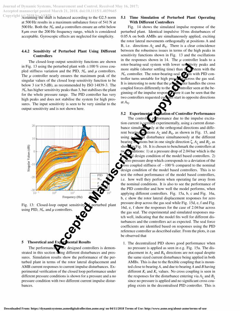
4.4.2 Sensitivity of Perturbed Plant Using DifferentControllers

The closed-loop output sensitivity functions are shownin Fig. 13 using the perturbed plant with ±100 % cross cou-pled stiffness variation and the PID, H∞ and µ controllers.The µ controller nearly ensures the maximum peak of thesingular values of the closed loop sensitivity function to bebelow 3 (or 9.5 dB), as recommended by ISO 14839-3. TheH∞ has higher sensitivity peaks than 3, but stabilises the plantfor the whole pressure range. The PID controller has veryhigh peaks and does not stabilise the system for high pres-sures. The input sensitivity is seen to be very similar to theoutput sensitivity and is not shown here.

10−1 100 101 102 103-30

-20

-10

0

10

20

PID

H∞

µ

Zone A

Frequency (Hz)

Sing

ular

Val

ues

(dB

)

Fig. 13: Closed-loop output sensitivity of perturbed plantusing PID, H∞ and µ controllers.

5 Theoretical and Experimental ResultsThe performance of the designed controllers is demon-

strated in this section using different disturbances and pres-sures. Simulation results show the performance of the per-turbed plant in terms of the rotor lateral displacement andAMB current responses to current impulse disturbances. Ex-perimental verification of the closed loop performance underdifferent pressure conditions is shown for a pressure and a nopressure condition with two different current impulse distur-bances.

5.1 Time Simulation of Perturbed Plant OperatingWith Different Controllers

Fig. 14 shows the simulated impulse response of theperturbed plant. Identical impulsive 10 ms disturbances of0.05 A on both AMBs are simultaneously applied, excitingthe rotor lateral movements orthogonally at positions A andB, i.e. directions Aζ and Bη. There is a clear coincidencebetween the robustness issues in terms of the high peaks insensitivity functions shown in Fig. 13 and the oscillationsin the responses shown in 14. The µ controller leads to arotor-bearing-seal system with lower sensitivity peaks andmore stable (shorter settling time) than the system with theH∞ controller. The rotor-bearing-seal system with PID con-troller turns unstable for high pressures across the gas seal.It is interesting to note that the µ controller handles the crosscoupled forces differently to the H∞ controller seen at the be-ginning of the impulse response. Here it can be seen that thetwo controllers requested currents start in opposite directionsat Aη.

5.2 Experimental Validation of Controller PerformanceThe controller performance due to the impulse excita-

tion current is verified experimentally, using a current distur-bance simultaneously at the orthogonal directions and diffe-rent bearing locations Aζ and Bη, as shown in Fig. 15, andusing a current disturbance simultaneously at the differentbearing locations but in one single direction ζ, Aζ and Bζ, asshown in Fig. 16. It is chosen to benchmark the controllers attwo conditions: 1) at a pressure drop of 2.04 bar which is thenominal design condition of the model based controllers. 2)at zero pressure drop which corresponds to a deviation of thecross coupled stiffness of −100 % compared to the nominaldesign condition of the model based controllers. This is totest the robust performance of the model based controllers,i.e. how well they perform when operating far away fromthe nominal conditions. It is also to see the performance ofthe PID controller and how well the model performs, whenapplying different controllers. Fig. 15a, b, c and Fig. 16a,b, c show the rotor lateral displacement responses for zeropressure drop across the gas seal while Fig. 15d, e, f and Fig.16d, e, f show the responses for the case of 2.04 bar acrossthe gas seal. The experimental and simulated responses ma-tch well, indicating that the model fits well for different dis-turbances and the controllers act as expected. The seal forcecoefficients are identified based on responses using the PIDreference controller as described ealier. From the plots, it canbe observed that

1. The decentralized PID shows good performance whenno pressure is applied as seen in e.g. Fig. 15a. The dis-placement in Aζ and Bη directions are not equal despitethe same sized current disturbance being applied in bothAMBs. This is due to the flexible coupling that is moun-ted close to bearing A, and due to bearing A and B havingdifferent Ki and Ks values. No cross coupling is seen inthe responses for the disturbance entering via Aζ and Bζ

since no pressure is applied and no significant cross cou-pling exists in the decentralised PID controller. This is

Accep

ted

Manus

crip

t Not

Cop

yedi

ted



Time (s)

Dis

plac

emen

t (m

)

(a)

Time (s)

Dis

plac

emen

t (m

)

(b)

Time (s)

Dis

plac

emen

t (m

)

(c)

Time (s)

Cur

rent

(A

)

(d)

Time (s)

Cur

rent

(A

)

(e)

Time (s)

Cur

rent

(A

)

(f)

Fig. 14: Impulse response of perturbed plant: (a) using PID controller; (b) using H∞ controller; and (c) using µ controller.(d), (e) and (f) show the control action in response to the impulse disturbance.

seen in Fig. 16a. Stability and performance issues ariseas the pressure is applied since this decentralized con-troller structure does not compensate for cross coupledseal forces. This is seen as oscillations in Fig. 15d.

2. The H∞ shows good performance for the nominal designpoint where a fixed pressure across the seal is applied asseen in Fig. 15e. The settling time of approximately0.03 s is very similar to the settling of the PID controllerwithout pressure applied. The displacement in Aζ and Bζ

is equal since the H∞ controller synthesis accounts forthe flexible coupling and the different Ki and Ks valuesof the two bearings. Stability problems can be detectedwhen using this controller for the case of zero pressureacross the seal. Such a claim can be reinforced by Fig.15b.

3. The µ controller shows very similar performance as theH∞ controller when the pressure drop across the gas sealis 2.04 bar. Such a similarity in terms of overshoot aswell as settling time is depicted in Fig. 15e, even thoughthe cross coupling effects due to the aerodynamic sealforces are handled slightly differently. For the case of nopressure drop across the seal, an improvement in termsof settling time, stabilization and reduction of oscilla-ting behaviour is seen when using the µ compared to theH∞ controller. Hence the µ controller is more robust tochanges of pressures across the seal.

6 ConclusionThis paper demonstrates the capabilities of three types

of controllers, both theoretically and experimentally, in ad-dressing and compensating for rotor lateral vibrations indu-ced by destabilising aerodynamic seal forces. Numericalsimulations of rotor lateral dynamics are carried out usingidentified mathematical models. Experiments are conductedusing the synthesised controllers applied to the test faci-lity. Comparison between theoretical and experimental re-sults agrees very well, allowing us to conclude that:

i) The designed H∞ controller shows significant per-formance improvements when the rotor-bearing-seal systemoperates close to design pressure conditions, i.e. pressuredrop across the gas seal around 2.04 bar. However, when thepressure drop across the seal changes from the nominal one,the performance of the controller is reduced, once the identi-fied model used to synthesize the controller is no longer ableto accurately predict the dynamics of the rotor-bearing-sealsystem (plant). Specifically, a decreased performance is ob-served when the pressure drop across the seal is lower thanthe nominal condition. ii) Using the perturbed plant formula-tion and µ synthesis to design robust controllers, it is shownto be possible to optimize and improve the worst case per-formance over a larger pressure range. The synthesised µcontroller is able to handle pressure variations better than theH∞ controller.

iii) Since the controller gains, and thus the direct stiff-ness and damping coefficients of the AMBs are cost parame-

Accep

ted

Manus

crip

t Not

Cop

yedi

ted



Time (s)

Dis

plac

emen

t (m

)

(a)

Time (s)

Dis

plac

emen

t (m

)

(b)

Time (s)

Dis

plac

emen

t (m

)

(c)

Time (s)

Dis

plac

emen

t (m

)

(d)

Time (s)

Dis

plac

emen

t (m

)

(e)

Time (s)

Dis

plac

emen

t (m

)

(f)

Fig. 15: Impulse response of plant in Aζ and Bη direction: (a) and (d) using PID controller; (b) and (e) using H∞ controller;and (c) and (d) using µ controller. (a), (b) and (c) show the response when no pressure is applied. (d), (e) and (f) showthe response when 2.04 bar pressure is applied. Simulated responses are shown as solid lines and experimental responsesare marked with ’- -’. Current impulsive setpoint disturbance from 0.05 s to 0.06 s is scaled in amplitude and shown as thedashed line ’Dis.’.

ters, they are kept approximately constant for all three typesof controllers, namely PID, H∞ and µ. The parameters sub-jected to changes are only the gas seals force coefficients dueto pressure drop variations. The seal force coefficients arequite high compared to the force coefficients of the AMBs.The theoretical and experimental investigations were carriedout in such a way to emphasise the difference in performanceof the controllers with similar gains. A slightly more realis-tic approach would be to increase the controller gain or thesize of the AMBs to obtain larger values of direct stiffnessand damping. This would immediately increase robustnessand stability followed by significant improvement in systemperformance.

iv) Finalizing, this paper has presented a structured wayto design robust controllers to deal with uncertain/varyingseal forces, including the tuning of the weighting functions.It is shown that the robust controller synthesis deals with fin-ding a non-conservative controller that will guarantee robustperformance while at the same time keeping the controllergains moderate. The method could potentially be implemen-ted in any AMB based systems subjected to seal or other fluidfilm forces.

A The System Matrices

The system matrices for the nominal plant in section 3and perturbed plant in 3.2 are given as

Accep

ted

Manus

crip

t Not

Cop

yedi

ted



Time (s)

Dis

plac

emen

t (m

)

(a)

Time (s)

Dis

plac

emen

t (m

)

(b)

Time (s)

Dis

plac

emen

t (m

)

(c)

Time (s)

Dis

plac

emen

t (m

)

(d)

Time (s)

Dis

plac

emen

t (m

)

(e)

Time (s)

Dis

plac

emen

t (m

)

(f)

Fig. 16: Impulse response of plant in Aζ and Bζ direction: (a) and (d) using PID controller; (b) and (e) using H∞ controller;and (c) and (d) using µ controller. (a), (b) and (c) show the response when no pressure is applied. (d), (e) and (f) showthe response when 2.04 bar pressure is applied. Simulated responses are shown as solid lines and experimental responsesare marked with ’- -’. Current impulsive setpoint disturbance from 0.05 s to 0.06 s is scaled in amplitude and shown as thedashed line ’Dis.’.

A =

−111 −166 130 84.6 8.07 −8.07 −2.81 −2.81

155 100 130 84.6 8.07 −8.07 −2.81 −2.81

−132 86.2 −261 67.7 −3.56 3.55 −4.62 −4.62

132 −86.2 −4.56 198 3.56 −3.55 4.62 4.62

86.7 −86.7 −52.5 −52.6 −180 −117 −0.11 −0.108

86.8 −86.8 −52.6 −52.6 118 180 −0.108 −0.106

64.1 −64.1 148 148 −0.934 0.861 182 −116

−64.1 64.1 −148 −148 0.86 −0.787 116 −182

B =

−1.716×10−2 5.470×10−2 −1.716×10−2 5.470×10−2

−1.716×10−2 5.469×10−2 −1.716×10−2 5.469×10−2

−3.508×10−2 −4.534×10−2 −3.508×10−2 −4.534×10−2

3.508×10−2 4.533×10−2 3.508×10−2 4.533×10−2

1.276×10−2 2.533×10−1 −1.276×10−2 −2.533×10−1

1.277×10−2 2.534×10−1 −1.277×10−2 −2.534×10−1

−2.265×10−1 −1.142×10−1 2.265×10−1 1.142×10−1

2.265×10−1 1.140×10−1 −2.265×10−1 −1.140×10−1

CT =

4.654×10−4 −3.601×10−4 4.654×10−4 −3.601×10−4

−4.653×10−4 3.602×10−4 −4.653×10−4 3.602×10−4

5.615×10−4 1.761×10−4 5.615×10−4 1.761×10−4

5.614×10−4 1.762×10−4 5.614×10−4 1.762×10−4

8.229×10−5 −1.635×10−4 −8.229×10−5 1.635×10−4

−8.238×10−5 1.634×10−4 8.238×10−5 −1.634×10−4

−1.828×10−4 9.214×10−6 1.828×10−4 −9.214×10−6

−1.828×10−4 9.211×10−6 1.828×10−4 −9.211×10−6

D =

0 0 0 0 0 0

0 0 0 0 0 0

0 0 0 0 0 0

0 0 0 0 0 0

0 0 0 0 0 0

0 0 0 0 0 0

Accep

ted

Manus

crip

t Not

Cop

yedi

ted



B∆ =

5.522×104 1.760×105

5.524×104 1.760×105

1.129×105 −1.459×105

−1.129×105 1.459×105

−2.736×10−3 −8.407×10−3

−2.729×10−3 −8.418×10−3

−5.877×10−3 −1.426×10−3

5.885×10−3 1.438×10−3

CT∆ =

−3.584×10−4 4.632×10−4

3.585×10−4 −4.631×10−4

1.753×10−4 5.588×10−4

1.754×10−4 5.588×10−4

1.049×10−12 1.432×10−13

−1.047×10−12 −1.446×10−13

−1.888×10−13 −3.178×10−13

−1.894×10−13 −3.160×10−13

∆ =

δ1 0

0 δ1

, |δ1|< 1

Accep

ted

Manus

crip

t Not

Cop

yedi

ted



B The Controller Statespace Matrices

C H∞ Controller

B =

−3.705 7.297 4.803 9.525

−6.587 −9.528 3.470×10−1 7.900

7.240 −3.190×10−1 −5.397 7.324

−2.300×10−1 9.377 −9.378 −7.295

2.246 −4.358 3.180×10−1 3.946

4.261 2.135 −3.835 2.420×10−1

1.622 −6.690×10−1 1.318 −1.769

6.680×10−1 1.634 1.733 1.285

9.743 −2.052×101 1.707 1.860×101

2.029×101 9.249 −1.812×101 1.437

−7.117 1.320 −6.848 6.251

1.305 7.034 6.111 6.741

1.140 1.800×10−2 −1.530 0.000

0.000 1.070 1.400×10−2 −1.543

−7.710×10−1 −2.930×10−1 −8.130×10−1 −1.990×10−1

−2.930×10−1 7.640×10−1 −1.940×10−1 7.690×10−1

5.460×10−1 1.270×10−1 −6.900×10−1 2.800×10−1

1.050×10−1 −4.990×10−1 2.670×10−1 7.020×10−1

−5.570×10−1 −1.560×10−1 −8.780×10−1 −1.410×10−1

−1.500×10−1 5.430×10−1 −1.430×10−1 8.640×10−1

A=

−6849.3 −2615.6 5494.9 3865.0 226.1 −714.3 −193.8 39.4 280.8 −1436.1 627.0 183.8 −52.3 −18.0 −9.7 108.3 −1.9 3.9 17.0 47.9

−2637.1 −9661.1 −4482.2 8558.9 1256.0 −458.0 −195.1 91.1 2437.9 −1086.2 493.3 31.9 −46.0 −113.6 44.1 −41.9 −7.2 4.4 27.7 4.4

2867.2 −4908.1 −18337.1 −4021.2 565.8 848.9 −230.3 −205.0 1177.0 1637.4 492.4 −444.8 83.0 −52.7 −45.0 44.3 3.7 8.7 19.6 6.4

4995.9 4908.7 991.2 −13554.0 −1101.1 691.8 275.6 −292.9 −2116.7 1450.1 −587.1 −627.2 59.1 110.7 64.2 58.7 11.2 −5.1 9.0 −25.8

−92.2 −5453.7 −10080.5 4238.0 884.4 139.5 −213.7 31.0 1659.0 192.6 424.8 12.8 11.7 −37.8 −30.8 −21.5 −5.6 −5.7 8.1 5.0

4284.0 98.0 −11323.7 −7356.3 −134.3 886.3 −29.9 −210.6 −180.2 1672.6 13.4 −421.6 34.3 10.7 −20.7 29.6 −5.9 5.2 4.8 −8.5

905.5 2846.6 2654.0 836.8 −215.2 −4.7 85.0 81.0 −373.6 33.0 −201.1 181.4 5.0 −0.1 −12.1 −14.4 3.0 0.7 −14.6 −1.5

−2152.2 1221.1 1966.8 2594.8 −2.9 −212.5 −78.7 86.0 −45.0 −371.5 174.7 203.1 1.4 4.6 −13.8 12.3 1.0 −2.8 −1.7 14.6

−2336.0 −39259.0 −63477.4 30444.0 6279.7 558.8 −1412.2 244.9 11134.6 537.4 2804.4 134.4 42.4 38.2 −172.0 −99.7 −47.4 −116.5 59.4 31.2

31197.4 −1519.0 −82916.0 −48458.1 −526.9 6404.2 −250.0 −1413.3 −455.8 11435.1 155.8 −2828.0 −68.6 35.8 −102.6 168.8 −122.3 45.7 30.1 −61.8

−8365.4 −23570.8 −33484.2 −6320.3 2108.9 477.7 −1070.3 −714.2 3599.2 530.9 1856.3 −1614.6 −48.6 182.0 −29.9 −192.9 −66.1 −45.0 87.5 −58.5

−18080.3 11373.7 17840.4 31392.2 417.0 −2094.2 −704.3 1089.2 434.3 −3602.4 1573.7 1896.0 181.2 42.5 206.0 −30.5 42.8 −63.3 58.7 88.1

−15812.7 5248.6 39169.0 22619.4 −108.1 −3054.9 37.0 736.6 −438.4 −4869.9 129.2 1340.8 −1180.7 −6.6 105.3 20.4 −1122.9 142.5 −149.9 112.4

−4656.2 −20018.9 −25149.6 12764.6 2976.6 −108.1 −734.7 27.2 4688.2 −432.2 1312.4 −154.2 8.9 −1193.0 16.0 −110.2 141.0 1125.3 119.7 160.4

−1241.8 9728.3 6788.2 11018.4 −272.9 −311.0 −31.0 541.3 −452.3 −516.6 133.4 738.4 66.7 −91.2 −1270.9 −26.7 211.4 54.5 −1177.5 282.7

7136.1 972.2 4538.6 −2527.4 −236.9 252.1 514.6 23.5 −399.6 419.6 −688.3 119.7 −94.5 −60.1 21.8 −1280.7 −50.6 220.7 −281.1 −1178.6

4139.6 −1767.8 −10424.0 −5244.3 107.7 762.1 −9.4 −174.2 242.0 1251.5 −14.6 −335.0 1190.5 −166.4 −222.4 −43.0 −221.1 20.2 −58.5 −74.6

−1499.6 −5223.3 −5212.1 3475.5 737.2 −109.7 −170.4 8.5 1196.1 −245.8 324.2 −18.3 −166.1 −1192.3 31.1 −240.6 −18.9 −216.6 67.3 −65.7

759.1 −3449.0 −4503.6 −3888.8 146.0 222.8 −30.5 −186.2 259.8 360.4 11.6 −311.1 139.4 −46.0 1168.3 229.4 −27.0 −76.6 −276.6 −44.2

−2590.8 −837.7 −1626.1 2232.7 207.4 −140.2 −180.4 33.2 333.4 −252.0 298.4 15.8 −38.5 −152.8 −228.8 1169.4 80.1 −24.6 46.9 −272.6

D =

0 0 0 0

0 0 0 0

0 0 0 0

0 0 0 0

CT =

−4.587×102 2.548×102 7.269×102 5.248×102

−3.563×102 −5.871×102 −6.740×102 9.188×102

9.618×102 −5.935×102 −1.936×103 1.277×103

1.820×102 2.838×102 −1.450×103 −6.449×102

1.234×101 8.350×101 1.754×101 −1.376×102

−8.619×101 1.218×101 1.407×102 1.652×101

3.338 4.289 6.950×10−1 5.429×101

−3.833 2.517 −5.538×101 6.740×10−1

1.044×101 1.366×102 3.993×101 −2.239×102

−1.430×102 1.081×101 2.313×102 3.845×101

1.189 −1.673 −6.310 −9.959×101

−7.620×10−1 −2.605 −1.024×102 6.775

4.032 −6.230×10−1 −9.047 −4.650×10−1

6.110×10−1 3.613 3.650×10−1 −8.645

−1.152 −3.520×10−1 −4.106 3.040

−3.320×10−1 1.244 3.121 3.726

2.648 −1.450×10−1 −4.128 1.846

−1.380×10−1 −2.493 1.818 4.064

3.620×10−1 −2.000×10−3 8.490×10−1 −3.036

1.600×10−2 −4.020×10−1 −3.132 −8.630×10−1

Accep

ted

Manus

crip

t Not

Cop

yedi

ted



D µ Controller

B =

0.000 0.000 0.000 1.000×10−3

0.000 0.000 0.000 0.000

5.988×101 1.966×102 2.715×101 3.150×102

−2.655×102 1.303×103 −3.392×102 1.572×103

−2.224×102 −9.787×101 −2.878×102 −1.945×102

9.787×102 1.046×103 1.129×103 1.264×103

4.725×101 8.134×102 −6.440×101 −1.320×103

2.685×102 5.001×103 −2.938×102 −5.984×103

−4.589×103 −2.247×103 5.369×103 2.704×103

7.822×102 3.594×102 −1.192×103 −6.008×102

2.000×10−3 0.000 0.000 0.000

0.000 2.000×10−3 0.000 0.000

0.000 0.000 2.000×10−3 0.000

0.000 0.000 0.000 2.000×10−3

−3.000×10−3 0.000 1.000×10−3 0.000

1.000×10−3 0.000 0.000 0.000

0.000 −3.000×10−3 0.000 1.000×10−3

0.000 1.000×10−3 0.000 0.000

1.000×10−3 0.000 −3.000×10−3 0.000

0.000 0.000 2.000×10−3 0.000

0.000 1.000×10−3 0.000 −3.000×10−3

0.000 0.000 0.000 2.000×10−3

−1.000×10−3 0.000 −1.000×10−3 0.000

0.000 1.000×10−3 0.000 1.000×10−3

A=

−0 0 0 0 0 0 0 0 0 0 0 0 0 0 0 0 0 0 0 0 0 0 0 0

0 −0 0 0 0 0 0 0 0 0 0 0 0 0 0 0 0 0 0 0 0 0 0 0

23688 7195 −23 −254 47 1 −6 6 2 2 0 0 0 0 0 −7001079 0 21573838 0 −7934556 0 25293464 −91276 −516528

128313 −6766 964 −710 34 −12 −23 23 7 7 0 0 0 0 0 −7002457 0 21568214 0 −7936117 0 25286871 −91335 −516385

−15809 −23777 −51 5 −56 273 3 −3 2 2 0 0 0 0 0 −14313495 0 −17882589 0 −16221961 0 −20965794 −443011 481953

116164 105845 42 4 −969 −766 −11 11 −11 −11 0 0 0 0 0 14313771 0 17876102 0 16222274 0 20958188 442991 −481793

−23280 −4112 −21 21 7 7 32 −330 0 0 0 0 0 0 0 5207601 0 99887417 0 −5901947 0 −117109388 0 0

−45096 −7620 −124 124 60 60 1211 −912 1 1 0 0 0 0 0 5210942 0 99919285 0 −5905734 0 −117146750 0 0

24898 36523 −57 57 −167 −167 5 −6 −926 −1224 0 0 0 0 0 −92418242 0 −45033594 0 104740676 0 52798006 0 0

−13123 −19218 −1 1 18 18 −3 3 336 38 0 0 0 0 0 92414117 0 44970403 0 −104736001 0 −52723920 0 0

0 0 0 0 0 0 0 0 0 0 0 0 0 0 0 0 0 0 0 0 0 0 0 0

0 0 0 0 0 0 0 0 0 0 0 0 0 0 0 0 0 0 0 0 0 0 0 0

0 0 0 0 0 0 0 0 0 0 0 0 0 0 0 0 0 0 0 0 0 0 0 0

0 0 0 0 0 0 0 0 0 0 0 0 0 0 0 0 0 0 0 0 0 0 0 0

1 −159 −0 0 −0 −1 0 0 0 0 −912 −446 −813 −568 −4410 −7446 −1656 −3092 −2447 −5066 −2240 −4400 −259 182

0 0 0 0 0 0 0 0 0 0 0 0 0 0 1024 0 0 0 0 0 0 0 0 0

−95 −206 −0 0 −0 −1 0 0 0 0 −689 −1090 −979 −1007 −1656 −3519 −5437 −9178 −2946 −6261 −3612 −7173 −233 332

0 0 0 0 0 0 0 0 0 0 0 0 0 0 0 0 1024 0 0 0 0 0 0 0

−14 −284 −0 0 −0 −1 0 0 −0 0 −992 −803 −1875 −1031 −2447 −4970 −2946 −5524 −7948 −14907 −4026 −7936 −412 319

0 0 0 0 0 0 0 0 0 0 0 0 0 0 0 0 0 0 1024 0 0 0 0 0

−161 −291 −0 0 −0 −1 0 0 0 0 −951 −1110 −1353 −1943 −2240 −4785 −3612 −6826 −4026 −8578 −8960 −16546 −319 465

0 0 0 0 0 0 0 0 0 0 0 0 0 0 0 0 0 0 0 0 1024 0 0 0

0 0 0 0 0 0 0 0 0 0 0 0 0 0 0 0 0 0 0 0 0 0 −2 0

0 0 0 0 0 0 0 0 0 0 0 0 0 0 0 0 0 0 0 0 0 0 0 −2

D =

0 0 0 0

0 0 0 0

0 0 0 0

0 0 0 0

CT =

−2.325×101 1.843×103 2.700×102 3.132×103

3.106×103 4.026×103 5.543×103 5.674×103

1.884 2.001 3.313 2.589

−4.456 −1.377 −7.122 −1.309

2.288 3.517 4.228 5.069

1.013×101 1.220×101 1.735×101 1.716×101

4.100×10−2 5.200×10−2 2.000×10−2 1.780×10−1

−2.070×10−1 2.180×10−1 2.250×10−1 −7.790×10−1

−9.600×10−2 3.960×10−1 1.169 4.860×10−1

5.500×10−2 8.800×10−2 2.170×10−1 1.150×10−1

1.781×104 1.346×104 1.936×104 1.858×104

8.702×103 2.128×104 1.568×104 2.167×104

1.587×104 1.912×104 3.661×104 2.642×104

1.109×104 1.966×104 2.012×104 3.793×104

5.502×104 3.234×104 4.778×104 4.374×104

1.101×105 6.871×104 9.705×104 9.343×104

3.234×104 7.508×104 5.753×104 7.053×104

6.038×104 1.439×105 1.079×105 1.333×105

4.778×104 5.753×104 1.241×105 7.861×104

9.892×104 1.223×105 2.558×105 1.675×105

4.374×104 7.053×104 7.861×104 1.439×105

8.592×104 1.401×105 1.550×105 2.878×105

5.056×103 4.553×103 8.049×103 6.224×103

−3.550×103 −6.490×103 −6.235×103 −9.079×103

Accep

ted

Manus

crip

t Not

Cop

yedi

ted



References[1] Fritz, R., 1970. “The effects of an annular fluid on the

vibrations of a long rotor, part 1theory”. Journal ofFluids Engineering, 92, pp. 923–929.

[2] Black, H., 1969. “Effects of hydraulic forces in annu-lar pressure seals on the vibrations of centrifugal pumprotors”. Journal of Mechanical Engineering Science,11(2), pp. 206–213.

[3] Black, H., and Jenssen, D., 1970. “Dynamic hybridproperties of annular pressure seals”. Journal of FluidsEngineering, 184, pp. 92–100.

[4] Childs, D. W., and Dressman, J. B., 1982. “Testingof turbulent seals for rotordynamic coefficients”. InProc. Workshop on Rotordynamic Instability Problemsin High-Performance Turbomachinery, NASA Conf.Publ. 2250, pp. 157–171.

[5] Nordmann, R., and Massmann, H., 1984. “Identifica-tion of dynamic coefficients of annular turbulent seals”.In Proc. Workshop on Rotordynamic Instability Pro-blems in High-Performance Turbomachinery, NASAConf. Publ. 2338, pp. 295–311.

[6] Baskharone, E., and Hensel, S., 1993. “Flow field inthe secondary, seal-containing passages of centrifugalpumps”. Journal of Fluids Engineering, 115, pp. 702–702.

[7] Schettel, J., and Nordmann, R., 2004. “Rotordynamicsof turbine labyrinth seals - a comparison of cfd mo-dels to experiments”. Imeche Conference Transactions,2004(2), pp. 13–22.

[8] Ishii, E., Chisachi, K., Kikuchi, K., and Ueyama, Y.,1997. “Prediction of rotordynamic forces in a labyrinthseal based on three-dimensional turbulent flow compu-tation”. Machine Elements and Manufacturing, 40(4),pp. 743–748.

[9] Rhode, D. L., Hensel, S. J., and Guidry, M. J., 1992.“Labyrinth seal rotordynamic forces using a three-dimensional navier-stokes code”. Journal of Tribology,114(4), p. 683.

[10] Hirs, G., 1973. “A bulk-flow theory for turbulence inlubricant films”. ASME J. Lubr. Technol, pp. 137–146.

[11] Childs, D., 1989. “Fluid-structure interaction forces atpump-impeller-shroud surfaces for rotordynamic cal-culations”. Journal of Vibration, Acoustics, Stress, andReliability in Design, 111, pp. 216–225.

[12] Nielsen, K. K., Jønck, K., and Underbakke, H., 2012.“Hole-pattern and honeycomb seal rotordynamic for-ces: Validation of cfd-based prediction techniques”.Journal of Engineering for Gas Turbines and Power,134(12), p. 122505.

[13] Marquette, O., Childs, D., and SanAndres, L., 1997.“Eccentricity effects on the rotordynamic coefficientsof plain annular seals: Theory versus experiment”.Journal of Tribology, 119(3), pp. 443–447.

[14] Hsu, Y., and Brennen, C., 2002. “Fluid flow equati-ons for rotordynamic flows in seals and leakage paths”.Journal of Fluids Engineering, 124(1), pp. 176–181.

[15] Kirk, R., and Guo, Z., 2004. “Calibration of labyrinthseal bulk flow design analysis predictions to cfd simu-

lation results”. In Eighth International Conference onVibrations in Rotating Machinery, pp. 3–12.

[16] Kocur, J. A., Nicholas, J. C., and Lee, C. C., 2007.“Surveying tilting pad journal bearing and gas laby-rinth seal coefficients and their effect on rotor stability”.In 36th Turbomachinery Symposium, TurbomachineryLaboratory, Texas A&M University, College Station,TX, September, pp. 10–13.

[17] San Andres, L., 2012. “Rotordynamic force coeffi-cients of bubbly mixture annular pressure seals”. Jour-nal of Engineering for Gas Turbines and Power, 134(2),p. 022503.

[18] Cole, M. O., Keogh, P. S., Sahinkaya, M. N., and Bur-rows, C. R., 2004. “Towards fault-tolerant active cont-rol of rotor–magnetic bearing systems”. Control Engi-neering Practice, 12(4), pp. 491–501.

[19] Balas, G. J., and Young, P. M., 1995. “Control de-sign for variations in structural natural frequencies”.Journal of Guidance, Control, and Dynamics, 18(2),pp. 325–332.

[20] Schonhoff, U., Luo, J., Li, G., Hilton, E., Nordmann,R., and Allaire, P., 2000. “Implementation results ofmu-synthesis control for an energy storage flywheeltest rig”. In Proceedings of ISMB8.

[21] Zhou, K., Doyle, J. C., Glover, K., et al., 1996. Robustand optimal control, Vol. 40. Prentice hall New Jersey.

[22] ISO, S., 2004. “Mechanical vibration-vibration ofrotating machinery equipped with active magneticbearings-part 3: Evaluation of stability margin”. ISO14839-3: 2006 (E).

[23] Cole, M., Chamroon, C., and Keogh, P., 2016. “H-infinity controller design for active magnetic bearingsconsidering nonlinear vibrational rotordynamics”. InProceedings of ISMB15.

[24] Balini, H., Witte, J., and Scherer, C. W., 2012. “Synt-hesis and implementation of gain-scheduling and lpvcontrollers for an amb system”. Automatica, 48(3),pp. 521–527.

[25] Mushi, S. E., Lin, Z., Allaire, P. E., and Evans, S.,2008. “Aerodynamic cross-coupling in a flexible rotor:Control design and implementation”. In Proceedings ofISMB11.

[26] Wurmsdobler, P., 1997. “State space adaptive cont-rol for a rigid rotor suspended in active magnetic be-arings”. PhD thesis, TU Wien.

[27] Lang, O., Wassermann, J., and Springer, H., 1996.“Adaptive vibration control of a rigid rotor supportedby active magnetic bearings”. Journal of engineeringfor gas turbines and power, 118(4), pp. 825–829.

[28] Hirschmanner, M., and Springer, H., 2002. “Adaptivevibration and unbalance control of a rotor supported byactive magnetic bearings”. In Proceedings of ISMB8.

[29] Lauridsen, J., and Santos, I., 2017. “Design of robustamb controllers for rotors subjected to varying and un-certain seal forces”. Mechanical Engineering Journal,pp. 16–00618.

[30] Lauridsen, J. S., and Santos, I. F., 2018. “On-site identi-fication of dynamic annular seal forces in turbo machi-

Accep

ted

Manus

crip

t Not

Cop

yedi

ted



nery using active magnetic bearings - an experimentalinvestigation”. Journal of Engineering for Gas Turbi-nes and Power.

[31] Voigt, A. J., Mandrup-Poulsen, C., Nielsen, K. K., andSantos, I. F., 2017. “Design and calibration of a fullscale active magnetic bearing based test facility for in-vestigating rotordynamic properties of turbomachineryseals in multiphase flow”. Journal of Engineering forGas Turbines and Power, 139(5), p. 052505.

[32] Voigt, A. J., 2016. “Towards identification of rotor-dynamic properties for seals in multiphase flow usingactive magnetic bearings. design and commissioning ofa novel test facility”. PhD thesis, Technical Universityof Denmark.

[33] Bleuler, H., Cole, M., Keogh, P., Larsonneur, R., Mas-len, E., Okada, Y., Schweitzer, G., and Traxler, A.,2009. Magnetic bearings: theory, design, and appli-cation to rotating machinery. Springer-Verlag BerlinHeidelberg.

[34] Childs, D. W., 1993. Turbomachinery rotordynamics:phenomena, modeling, and analysis. Wiley New York.

[35] Nelson, H., 1980. “A finite rotating shaft element usingtimoshenko beam theory”. Journal of Mechanical De-sign, 102(4), pp. 793–803.

[36] Skogestad, S., and Postlethwaite, I., 2007. Multiva-riable feedback control: analysis and design, Vol. 2.Wiley New York.

[37] Voigt, A. J., Lauridsen, J. S., Poulsen, C. M., Nielsen,K. K., and Santos, I. F., 2016. “Identification of para-meters in active magnetic bearing systems”. In Procee-dings of ISMB15.

Accep

ted

Manus

crip

t Not

Cop

yedi

ted



Documents

Design of Active Magnetic Bearing Controllers for Rotors