Design Optimization of an Electric Motor - uni-sofia.bgecmimw2016.fmi.uni-sofia.bg/final_reports/report_group_3.pdf · ECMI Modelling Week, July 17–24, 2016, Soﬁa, Bulgaria Group

ECMI Modelling Week, July 17–24, 2016, Sofia, Bulgaria

Group 3

Design Optimization of an ElectricMotor

Robert BauerTechnische Universitat Dresden, [email protected]

Pedro Rodriguez-BarbeitoUniversity of Santiago de Compostela, [email protected]

Anne Ryelund NielsenTechnical University of Denmark, [email protected]

Szymon SobieszekWroclaw University of Science and Technology, [email protected]

Lea Miko VersbachLund University, [email protected]

Instructor: Peter GanglJohannes Kepler University Linz, [email protected]

1

2 Design Optimization of an Electric Motor

Abstract. The optimization of electrical machines is of utter impor-tance in industry. In this project, we consider the design optimizationof an electric motor consisting of different components. The efficiencyof the motor heavily depends on its geometry. For a fixed geometry,the arising magnetic field can be computed as the solution of a partialdifferential equation (PDE). The goal of the project is to determine theshapes and sizes of specific parts of the electric motor such that thecorresponding magnetic field yields an optimal behavior with respect tosome prescribed criteria (e.g., transmitted power, reduction of noise andvibration).

3.1 Introduction

In industry, the optimization of electrical machines is of great importance. In thisproject, we consider the design optimization of an electric motor which consistsof the following components:

• Stator, consisting of ferromagnetic material (outer part),

• Rotor, consisting of ferromagnetic material (inner part),

• Air regions,

• Coils (in the stator),

• Permanent magnets possible.

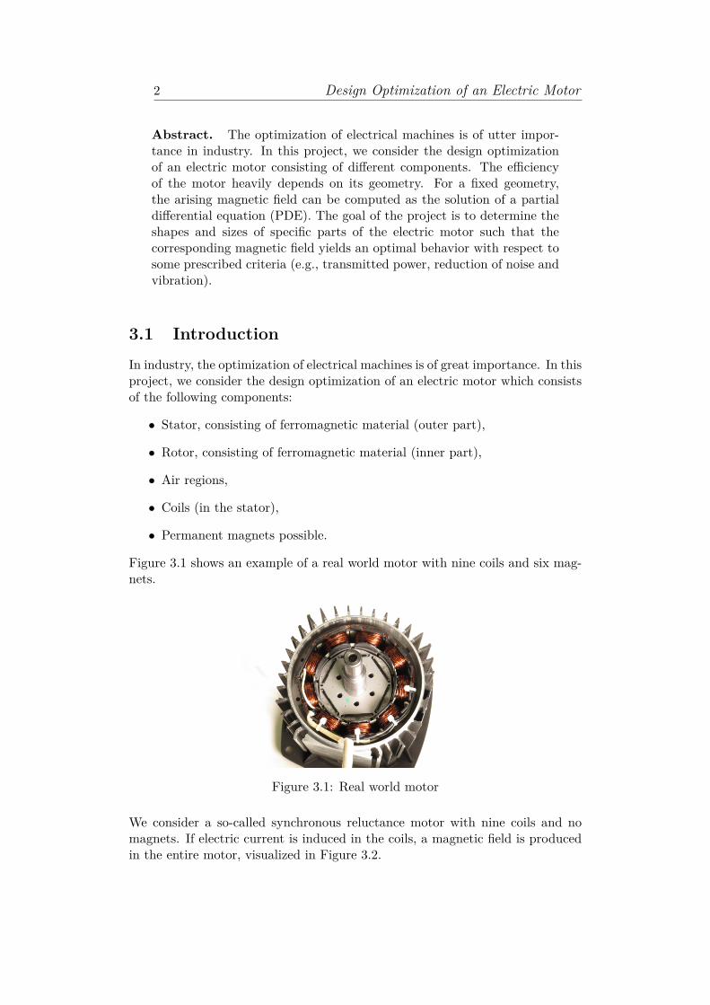
Figure 3.1 shows an example of a real world motor with nine coils and six mag-nets.

Figure 3.1: Real world motor

We consider a so-called synchronous reluctance motor with nine coils and nomagnets. If electric current is induced in the coils, a magnetic field is producedin the entire motor, visualized in Figure 3.2.

3 ECMI Modelling Week 2016, Sofia, Bulgaria

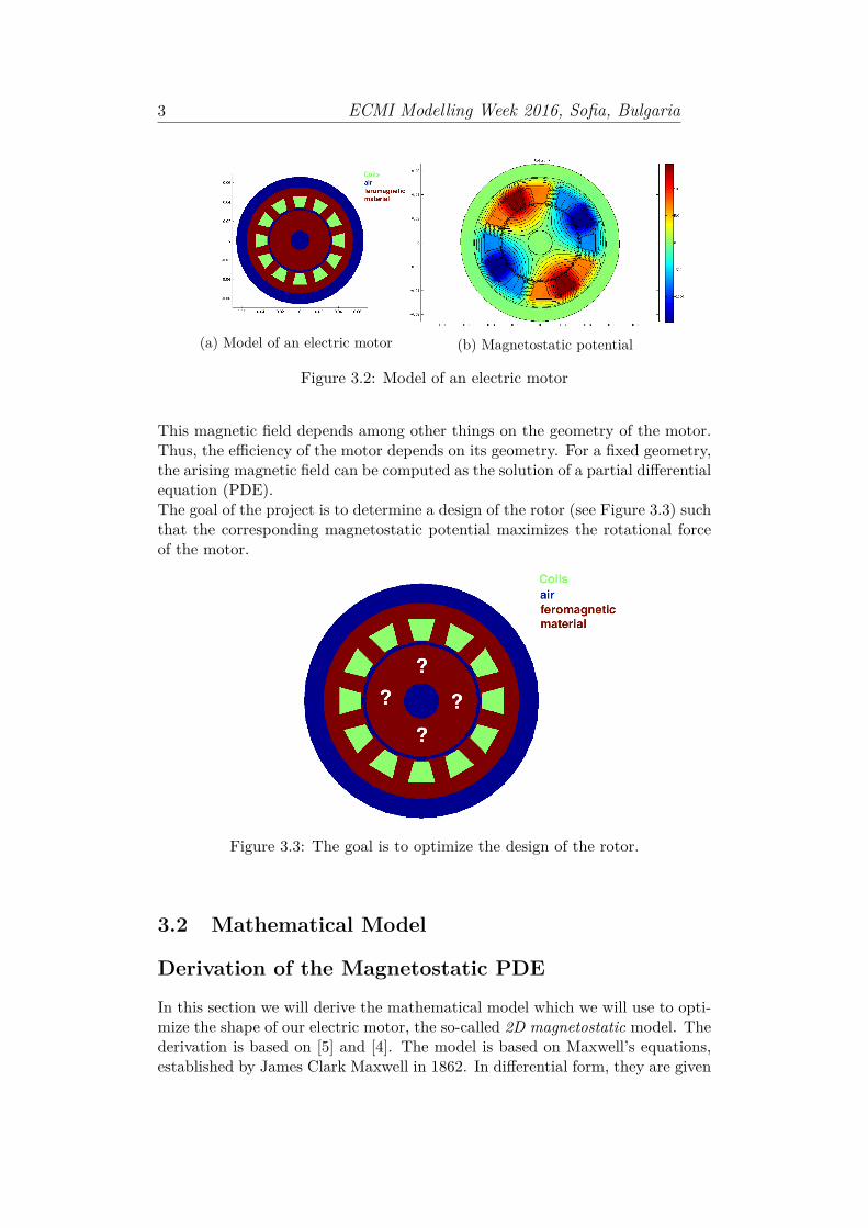
(a) Model of an electric motor (b) Magnetostatic potential

Figure 3.2: Model of an electric motor

This magnetic field depends among other things on the geometry of the motor.Thus, the efficiency of the motor depends on its geometry. For a fixed geometry,the arising magnetic field can be computed as the solution of a partial differentialequation (PDE).The goal of the project is to determine a design of the rotor (see Figure 3.3) suchthat the corresponding magnetostatic potential maximizes the rotational forceof the motor.

Figure 3.3: The goal is to optimize the design of the rotor.

3.2 Mathematical Model

Derivation of the Magnetostatic PDE

In this section we will derive the mathematical model which we will use to opti-mize the shape of our electric motor, the so-called 2D magnetostatic model. Thederivation is based on [5] and [4]. The model is based on Maxwell’s equations,established by James Clark Maxwell in 1862. In differential form, they are given


by:

∇×H = J + ∂D

∂t,

∇× E = −∂B∂t,

∇ ·B = 0,∇ ·D = ρ.

Here, for differentiable vector fields F : Ω ⊂ R3 → R3 and a spatial variablex = (x1, x2, x3) ∈ Ω, we used the following operators in cartesian coordinates

∇× F :=

∂F3/∂x2 − ∂F2/∂x3

∂F1/∂x3 − ∂F3/∂x1

∂F2/∂x1 − ∂F1/∂x2

,

which is called the curl or rotation of F and is also a vector field and

∇ · F := divF := ∂F1∂x1

+ ∂F2∂x2

+ ∂F3∂x3

,

the divergence of F , which is a scalar field. The physical quantities involved are

• H ... magnetic field or magnetic excitation [A/m],

• B ...magnetic induction or magnetic flux density [V s/m2],

• E ... electric field [V/m],

• D ... electric flux density or electric induction [As/m2],

• J ... (surface) current density [As/m2] and

• ρ ... (volume) charge density [As/m3].

All these functions are time dependent to the time t ∈ R and of course, H,B,E,Dand J are vector fields and ρ is a scalar field. For uniqueness of our system ofequations we assume the following material laws:

B =µH,D =εE,J =σE + Ji,

involving

• µ ... magnetic permeability [V s/Am]

• ε ... electric permittivity [As/V m]

• σ ... electric conductivity [A/Vm]


• Ji ... impressed current density [A/m2].

In general, µ and ε are non-linear rank 2 tensors, depending on space, time andthe fields E and H. But in our problem, these quantities are scalar and weconsider isotropic, materials without hysteresis and assume

B = µ(x, |H|)H.

Now we can consider the magnetic reluctivity ν defined by,

H = ν(x, |B|)B.

In our case, we consider only non-conducting regions, i.e. σ = 0 and we furtherassume that all fields are time independent, i.e. ∂

∂t = 0. The equations forthe magnetic and electric fields are therefore decoupled into two independentsystems and we are just looking at the simplified magnetostatic equations:

∇×H = Ji

∇ ·B = 0H = ν(x, |B|)B.

Because of the divergence free magnetic flux density B, there exists a vectorpotential A, depending on a space variable x, such that B = ∇×A. Now we got

Ji = ∇×H= ∇× [ν(x, |B|)B]= ∇× [ν(x, |∇ ×A|)∇×A].

In our project we deal with the magnetostatic equation only in an open andbounded 2D domain Ω ⊂ R2, which describe the geometry of the electric motor.In addition the ferromagnetic material regions Ωferro and air regions Ωair (alsoincluding the coils) are disjoint, i.e Ω = Ωferro∪ Ωair, Ωferro∩Ωair = ∅ and we saythat ν only depends on the kind of material:

ν(x, |∇ ×A|) =ν0 if x ∈ Ωair

ν(|∇ ×A|) if x ∈ Ωferro.

Furthermore we say that the current density Ji is perpendicular to the magneticfield H, and so for x = (x1, x2) we have

Ji =

00

Ji3(x1, x2)

, H =

H1(x1, x2)H2(x1, x2)

0

.

From the B-H-relation we also get

B =

B1(x1, x2)B2(x1, x2)

0

.


With the identity ∇×A = B we get

0 = B3 = (∇×A)3 = ∂2A1 − ∂1A2,

and to fulfill this we use the approach

A =

00

A3(x1, x2)

.

Now we use the notation u := A3, J := Ji3 and find

|∇ ×A| = |

∂2A3−∂1A3

0

| = |∇u|.Now we can simplify our magnetostatic equation as follows:

Ji =

00

Ji3(x1, x2)

= ∇× [ν(x, |∇ ×A|)∇×A]

= ∇×

ν(x, |∇u|)∂2u−ν(x, |∇u|)∂1u

0

=

00

∂1[−ν(x, |∇u|)∂1u]− ∂2[ν(x, |∇u|)∂2u]

=

00

−∇ · [ν(x, |∇u|)∇u]

,

and get that

−div[ν(x, |∇u|)∇u] = J. (3.1)

In our model, the domain Ω is a circle where the electric motor Ωmotor is con-tained, i.e Ωmotor ⊂ Ω and

dist(Ωmotor, ∂Ω) > 0.

It can be shown that the condition

u = 0 on ∂Ω (3.2)

implies this other boundary condition

B · n = 0 on ∂Ω, (3.3)

which is the actual boundary condition that we want to impose. Combiningthis statement with (3.1) and the continuity of u and the fluxes ν ∂u∂n across the


material interfaces Ωferro, we can formulate the mathematical problem in theclassical sense:

Find u ∈ C2(Ωair ∪ Ωferro) ∩ C(Ω) such that

−div [ν(x, |∇ u|)∇u(x1, x2)] = J in Ω, (3.4a)u = 0 on ∂Ω, (3.4b)

JuK = 0 on Ωair ∩ Ωferro (3.4c)

Jν(x,∇u)∂u∂n

K = 0 on Ωair ∩ Ωferro (3.4d)

where we denote by JvK the jump of a function v across the interface Ωair∩Ωferro.

Weak Formulation of the Magnetostatic PDE

To give a weak formulation of the problem in (3.4) we start multiplying equation(3.4a) time a test function, v ∈ H1

0 (Ω), and integrating it over the domain, whichyields: ∫

Ω−div [ν(x, |∇ u|)∇u(x1, x2)] v dΩ =

∫ΩJv dΩ (3.5)

We can use use Green’s identity, which stands that for any two given fields,ψ, φ ∈ C2(Ω) the following equality, where n is the outer normal vector for Ω,holds ∫

φ divψ dΩ +∫ψ · ∇φ dΩ =

∫∂Ω

(n ·ψ) φ dΓ. (3.6)

Using it in (3.5) for ψ = ν(x, |∇ u|)∇u(x1, x2) and φ = v, we get the following:∫Ων ∇u(x1, x2)∇v(x1, x2) dΩ =

∫ΩJv(x1, x2) dΩ+

∫∂Ω

n·ν ∇u(x1, x2)v(x1, x2) dΓ.(3.7)

Then we can write a weak formulation for problem (3.4), which reads:

Find u ∈ H1(Ω) with u = 0 over ∂Ω such that∫Ων(x, |∇ u|)∇u(x1, x2)∇v(x1, x2) dΩ =

∫ΩJv(x1, x2) dΩ, (3.8)

∀v ∈ H10 (Ω).

The weak formulation of the equation is important since it is the starting pointto apply the Finite Element Method, which is the method used by the Matlab’ssolver to solve these kinds of PDEs.

Calculation of the Torque

We have reached a way to calculate the magnetic field generated by our electricmotor, nevertheless, the aim of the project is to optimize the force generated by


this magnetic field so we should be able to calculate this force.

This force we are talking about is called Torque and in our case, It’s defined asfollows:

T = 1µ0

∫Γ0∇uTQ(x)∇u dΓ0, (3.9)

being

Q(x) = 1√x2

1 + x22

x1x2x2

2−x21

2x2

2−x21

2 −x1x2

(3.10)

and Γ0 a circle standing in the middle of the air gap between the rotor and thestator.

This formula can be deduced from the general torque formula which reads

T = F× ~OP

when appling a force F on a given point P from a fixed one O. And using theMaxwell stress tensor. More information about this deduction can be consultedin [3].

3.3 Forward Problem

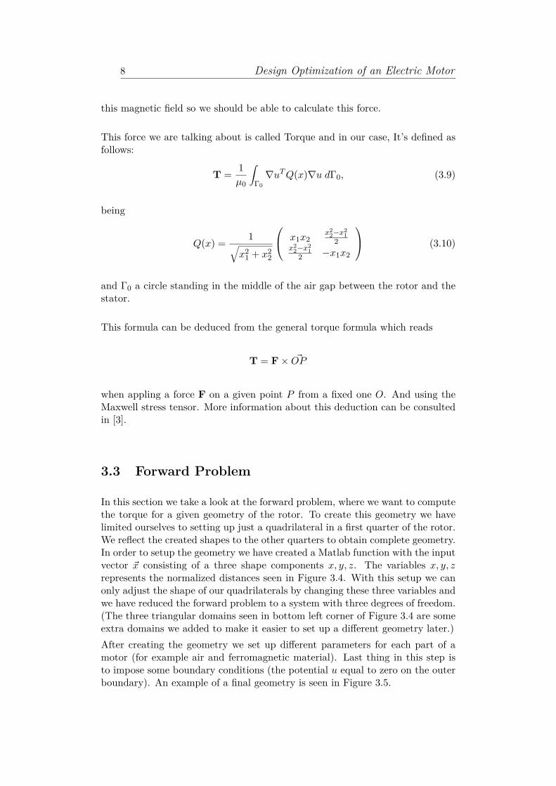
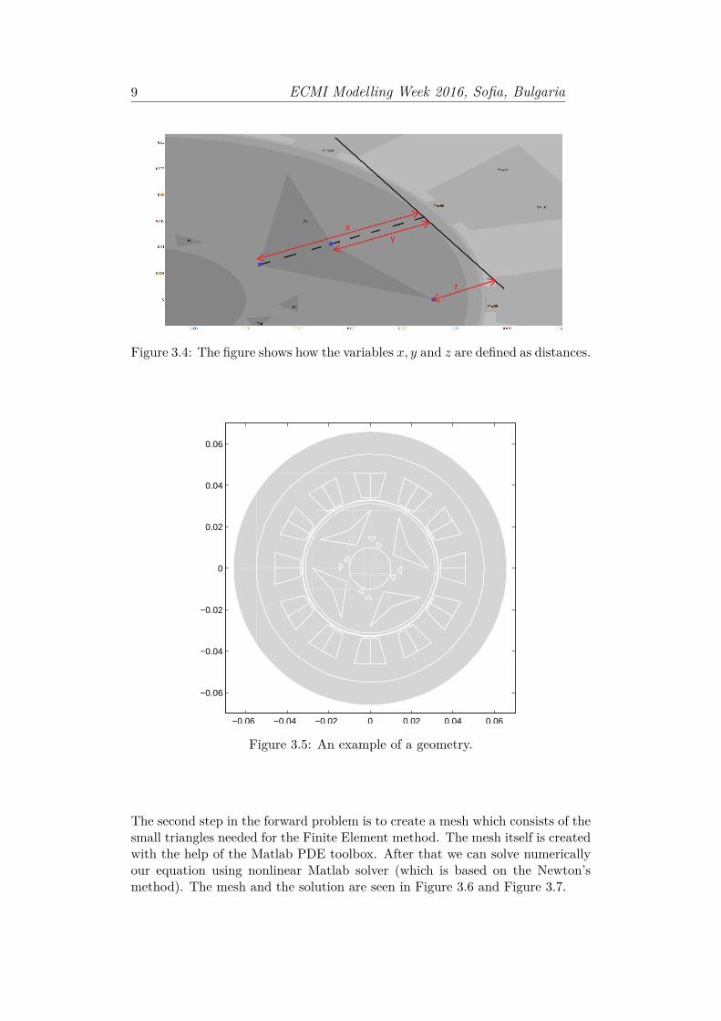
In this section we take a look at the forward problem, where we want to computethe torque for a given geometry of the rotor. To create this geometry we havelimited ourselves to setting up just a quadrilateral in a first quarter of the rotor.We reflect the created shapes to the other quarters to obtain complete geometry.In order to setup the geometry we have created a Matlab function with the inputvector ~x consisting of a three shape components x, y, z. The variables x, y, zrepresents the normalized distances seen in Figure 3.4. With this setup we canonly adjust the shape of our quadrilaterals by changing these three variables andwe have reduced the forward problem to a system with three degrees of freedom.(The three triangular domains seen in bottom left corner of Figure 3.4 are someextra domains we added to make it easier to set up a different geometry later.)After creating the geometry we set up different parameters for each part of amotor (for example air and ferromagnetic material). Last thing in this step isto impose some boundary conditions (the potential u equal to zero on the outerboundary). An example of a final geometry is seen in Figure 3.5.


Figure 3.4: The figure shows how the variables x, y and z are defined as distances.

−0.06 −0.04 −0.02 0 0.02 0.04 0.06

−0.06

−0.04

−0.02

0

0.02

0.04

0.06

Figure 3.5: An example of a geometry.

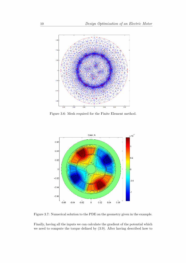
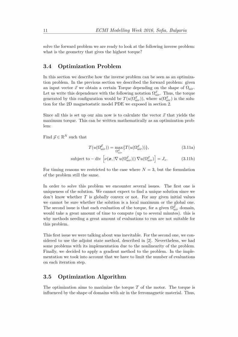
The second step in the forward problem is to create a mesh which consists of thesmall triangles needed for the Finite Element method. The mesh itself is createdwith the help of the Matlab PDE toolbox. After that we can solve numericallyour equation using nonlinear Matlab solver (which is based on the Newton’smethod). The mesh and the solution are seen in Figure 3.6 and Figure 3.7.


Figure 3.6: Mesh required for the Finite Element method.

Figure 3.7: Numerical solution to the PDE on the geometry given in the example.

Finally, having all the inputs we can calculate the gradient of the potential whichwe need to compute the torque defined by (3.9). After having described how to


solve the forward problem we are ready to look at the following inverse problem:what is the geometry that gives the highest torque?

3.4 Optimization Problem

In this section we describe how the inverse problem can be seen as an optimiza-tion problem. In the previous section we described the forward problem: givenan input vector ~x we obtain a certain Torque depending on the shape of Ωair.Let us write this dependence with the following notation Ω~x

air. Thus, the torquegenerated by this configuration would be T (u(Ω~x

air)), where u(Ω~xair) is the solu-

tion for the 2D magnetostatic model PDE we exposed in section 2.

Since all this is set up our aim now is to calculate the vector ~x that yields themaximum torque. This can be written mathematically as an optimization prob-lem:

Find ~p ∈ RN such that

T (u(Ω~pair)) = max

Ω~xair

T (u(Ω~xair)), (3.11a)

subject to− div[ν(x, |∇ u(Ω~x

air)|)∇u(Ω~xair)

]= Jz. (3.11b)

For timing reasons we restricted to the case where N = 3, but the formulationof the problem still the same.

In order to solve this problem we encounter several issues. The first one isuniqueness of the solution. We cannot expect to find a unique solution since wedon’t know whether T is globally convex or not. For any given initial valueswe cannot be sure whether the solution is a local maximum or the global one.The second issue is that each evaluation of the torque, for a given Ω~x

air domain,would take a great amount of time to compute (up to several minutes). this iswhy methods needing a great amount of evaluations to run are not suitable forthis problem.

This first issue we were talking about was inevitable. For the second one, we con-sidered to use the adjoint state method, described in [2]. Nevertheless, we hadsome problems with its implementation due to the nonlinearity of the problem.Finally, we decided to apply a gradient method to the problem. In the imple-mentation we took into account that we have to limit the number of evaluationson each iteration step.

3.5 Optimization Algorithm

The optimization aims to maximize the torque T of the motor. The torque isinfluenced by the shape of domains with air in the ferromagnetic material. Thus,


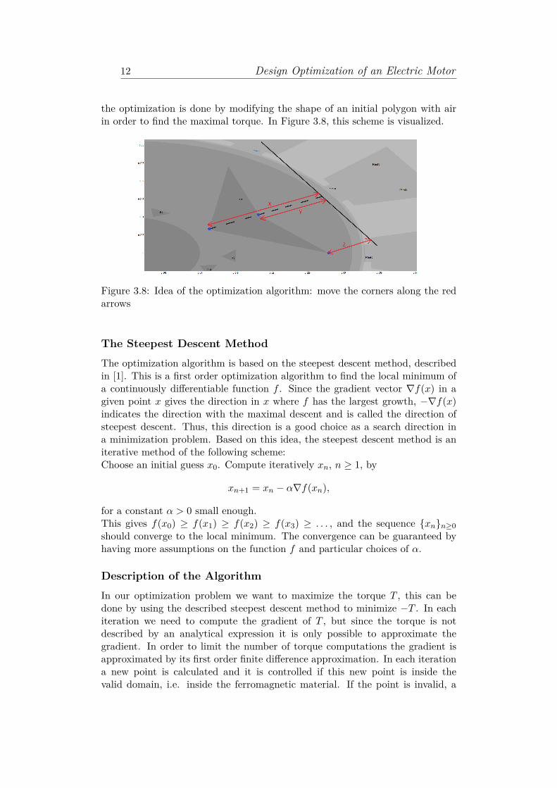
the optimization is done by modifying the shape of an initial polygon with airin order to find the maximal torque. In Figure 3.8, this scheme is visualized.

Figure 3.8: Idea of the optimization algorithm: move the corners along the redarrows

The Steepest Descent Method

The optimization algorithm is based on the steepest descent method, describedin [1]. This is a first order optimization algorithm to find the local minimum ofa continuously differentiable function f . Since the gradient vector ∇f(x) in agiven point x gives the direction in x where f has the largest growth, −∇f(x)indicates the direction with the maximal descent and is called the direction ofsteepest descent. Thus, this direction is a good choice as a search direction ina minimization problem. Based on this idea, the steepest descent method is aniterative method of the following scheme:Choose an initial guess x0. Compute iteratively xn, n ≥ 1, by

xn+1 = xn − α∇f(xn),

for a constant α > 0 small enough.This gives f(x0) ≥ f(x1) ≥ f(x2) ≥ f(x3) ≥ . . . , and the sequence xnn≥0should converge to the local minimum. The convergence can be guaranteed byhaving more assumptions on the function f and particular choices of α.

Description of the Algorithm

In our optimization problem we want to maximize the torque T , this can bedone by using the described steepest descent method to minimize −T . In eachiteration we need to compute the gradient of T , but since the torque is notdescribed by an analytical expression it is only possible to approximate thegradient. In order to limit the number of torque computations the gradient isapproximated by its first order finite difference approximation. In each iterationa new point is calculated and it is controlled if this new point is inside thevalid domain, i.e. inside the ferromagnetic material. If the point is invalid, a


new iteration point is calculated with decreased step size α. If a valid iterationpoint is found, the function values at both points are compared and only adecreasing function value for each iteration step is accepted. Finally, the gradientof the torque in the new iteration point is approximated. The algorithm stops,if the distance between two successive iteration points is smaller than a giventolerance (0.01) and we say that the algorithm converged. The algorithm doesnot converge, if the maximal number of iterations (20) is exceeded. A schematicdescription of the algorithm is listed below.

• given starting configuration x0, tolerance tol and step size α

• calculate T (x0), approximate ∇T (x0)

• while i < maxiter

– i = i+ 1– xi = xi−1 + α∇T (xi−1)– while xi is invalid∗ α = α

2∗ compute xi = xi−1 + α∇T (xi−1)

– calculate T (xi)– while T (xi) < T (xi−1)∗ α = α

2∗ compute xi = xi−1 + α∇T (xi−1)

– approximate ∇T (xi)– break if ‖xi − xi−1‖ < tol

3.6 Numerical Results, Interpretation and Conclu-sion

In this section we will present the numerical results obtained by applying thedescribed optimization routine. We conducted several numerical experiments,common to all of them was the fact that the z-value was fixed. This was doneto further reduce the degrees of freedom in our problem and thereby reducingthe computational time. Even with this simplification of the problem, eachnumerical experiment lasted up to 30 minutes. From the numerical experimentswith different initial configurations, we saw some tendencies: often the algorithmconverges after a couple of iterations to a local optimum, which is very close to theinitial conditions. But for some initial configurations the optimization algorithmmanages to find a local optimum further away from the initial conditions. Someof these results are listed in Table 3.1.For all the experiments listed in Table 3.1 we see that the torque is increasedapproximately 10% from the initial to the optimized configuration. In orderto compare the optimized configurations we have plotted the numerical solu-tions to the PDE on the initial- and optimized geometry for each of the three


Table 3.1: Selected numerical results

Initial configuration Optimized configuration No. iterations

Experiment 1x0 = 0.2 xopt = 0.7212y0 = 0.1 yopt = 0.6212 6 iterationsT0 = 0.002784 Topt = 0.003011



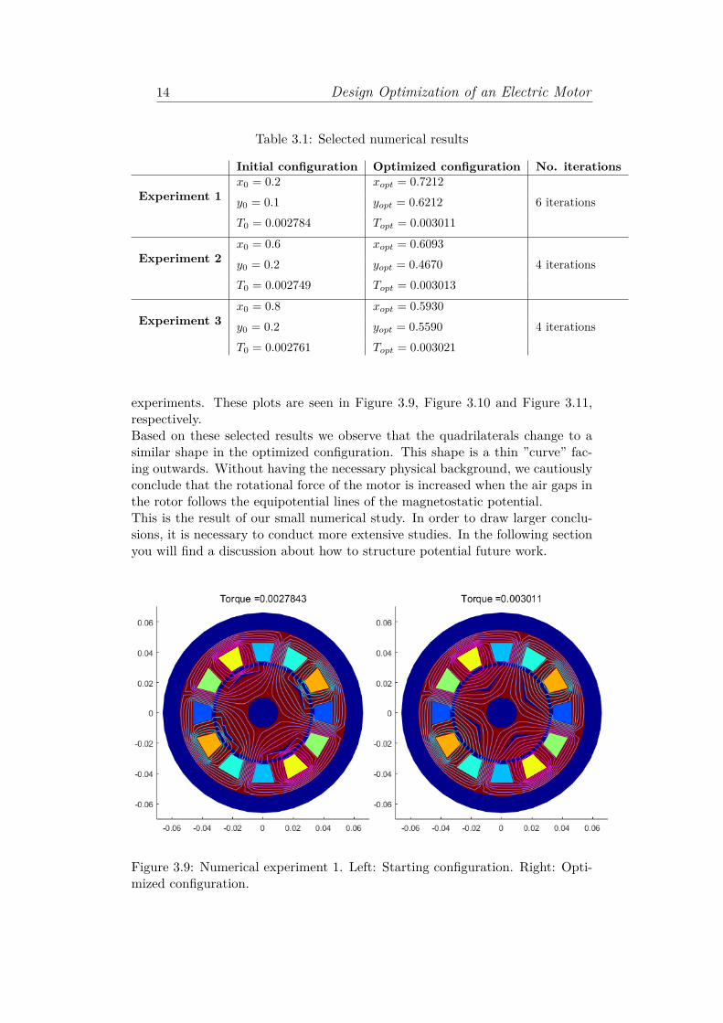
experiments. These plots are seen in Figure 3.9, Figure 3.10 and Figure 3.11,respectively.Based on these selected results we observe that the quadrilaterals change to asimilar shape in the optimized configuration. This shape is a thin ”curve” fac-ing outwards. Without having the necessary physical background, we cautiouslyconclude that the rotational force of the motor is increased when the air gaps inthe rotor follows the equipotential lines of the magnetostatic potential.This is the result of our small numerical study. In order to draw larger conclu-sions, it is necessary to conduct more extensive studies. In the following sectionyou will find a discussion about how to structure potential future work.

Figure 3.9: Numerical experiment 1. Left: Starting configuration. Right: Opti-mized configuration.


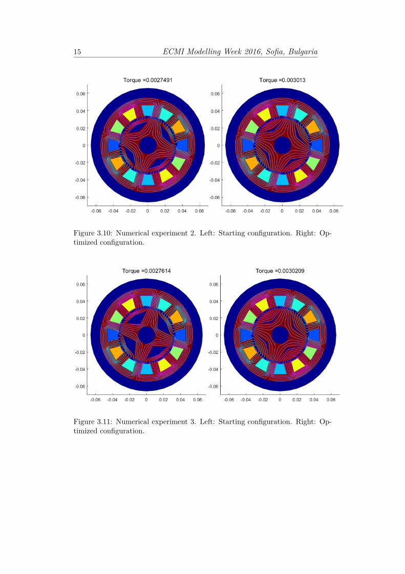
Figure 3.10: Numerical experiment 2. Left: Starting configuration. Right: Op-timized configuration.

Figure 3.11: Numerical experiment 3. Left: Starting configuration. Right: Op-timized configuration.


3.7 Future Work

Due to the limited amount of time for this project, some questions regarding thetopic remain open for future work.

• This project was solved by using the PDE toolbox in MATLAB. Doingso, we encountered a number of drawbacks, which lead to some limitationsin the solution. For example, the automatic numeration of the domainsled to a fixed number of possible polygons, which is not desireable in theoptimization. Thus, it would be of andvantage to use other packages orother programming languages to solve the PDE and to compute the torque.

• The optimization algorithm we used is based on a steepest descent method.There might exist more efficient and faster optimization algorithms whichare applicable to the given problem.

• I this project, the given polygons have a maximum of six degrees of freedomto change their shape. An improvement would be to extend this numberand compare the efficiency of the optimization algorithm.


Bibliography

[1] Lars-Christer Boiers. Mathematical Methods of Optimization. Studentlitter-atur AB, Lund, 2010.

[2] Peter W. Christensen & A. Klarbring. An introduction to structural opti-mization. Solid Mechanics and its Applications V.153 Springer, 2009.

[3] Elisabeth Frank & Walter Zulehner. Free-form Optimization of Electric Ma-chines based on Shape Derivatives(Master Thesis). Johannes Kepler Univer-sity, Linz, 2010.

[4] Peter Gangl & Ulrich Langer. Topology Optimization in Electrical Engineer-ing(Master Thesis). Johannes Kepler University, Linz, 2012.

[5] Clemens Pechstein & Ulrich Langer Multigrid-Newton-Methods for Nonlin-ear Magnetostatic Problems(Master Thesis). Johannes Kepler University,Linz, 2004.

Documents

Design Optimization of an Electric Motor - uni-sofia.bgecmimw2016.fmi.uni-sofia.bg/final_reports/report_group_3.pdf · ECMI Modelling Week, July 17–24, 2016, Soﬁa, Bulgaria Group