Embed Size (px)
Citation preview

Clemson UniversityTigerPrints
All Theses Theses
8-2013
DESIGN OPTIMIZATION OFGEOMETRICAL PARAMETERS ANDMATERIAL PROPERTIES OF VIBRATINGBIMORPH CANTILEVER BEAMS WITHSOLID AND HONEYCOMB SUBSTRATESFOR MAXIMUM ENERGY HARVESTEDJasmin AdesharaClemson University, [email protected]
Follow this and additional works at: https://tigerprints.clemson.edu/all_theses
Part of the Mechanical Engineering Commons
This Thesis is brought to you for free and open access by the Theses at TigerPrints. It has been accepted for inclusion in All Theses by an authorizedadministrator of TigerPrints. For more information, please contact [email protected].
Recommended CitationAdeshara, Jasmin, "DESIGN OPTIMIZATION OF GEOMETRICAL PARAMETERS AND MATERIAL PROPERTIES OFVIBRATING BIMORPH CANTILEVER BEAMS WITH SOLID AND HONEYCOMB SUBSTRATES FOR MAXIMUMENERGY HARVESTED" (2013). All Theses. 1717.https://tigerprints.clemson.edu/all_theses/1717

DESIGN OPTIMIZATION OF GEOMETRICAL PARAMETERS AND MATERIAL
PROPERTIES OF VIBRATING BIMORPH CANTILEVER BEAMS WITH SOLID
AND HONEYCOMB SUBSTRATES FOR MAXIMUM ENERGY HARVESTED
________________________________________________________________________
A Thesis
Presented to
the Graduate School of
Clemson University
________________________________________________________________________
In Partial Fulfillment
of the Requirements for the Degree
Master of Science
Mechanical Engineering
________________________________________________________________________
by
Jasmin Adeshara
August 2013
________________________________________________________________________
Accepted by:
Dr. Lonny L. Thompson, Committee Chair
Dr. Georges M. Fadel
Dr. Huijuan Zhao

ii
ABSTRACT
The objective of this thesis is to maximize the energy harvested from a vibrating bimorph
cantilever beam by optimizing the geometrical parameters and the material properties of
the piezoelectric beam. A three-dimensional finite element (FEA) model is developed to
design a vibrating bimorph cantilever beam for energy harvesting. The reference
piezoelectric material used in the design is Lead Zirconate Titanate (PZT-5H) and the
substrate sandwiched between the two piezoelectric plates is brass. Three types of models
are analyzed and compared in this work by modifying the brass substrate geometry- a
solid homogenous substrate, a regular honeycomb substrate and an auxetic honeycomb
substrate. Complete transversely isotropic elastic and piezoelectric properties are
assigned to the bimorph layers. A time harmonic pressure load is applied to the top
surface of the beam that results in electrical-mechanical coupling by vibration. The
electric potential on the surfaces of the bimorph piezoelectric beam is used to compute
voltage generated.
Also in this thesis, an automated design workflow has been set-up to solve an
optimization problem by integrating ABAQUS 6.10, the commercial finite element
package with the commercial optimization software package VisualDOC 7.1. The
optimizer, Non-dominated Sorting Genetic Algorithm II (NSGAII), depends on the
number of population, iterations, probability of cross over and mutations.

iii
The first objective of this work is to compare the finite element analysis results of the
bimorph cantilever beams with these three substrates for similar loading and boundary
conditions. The thickness of the substrates and the material properties are maintained
equal for all three models. The second objective is to optimize the thicknesses of the PZT
plates ‘tp’ and the relative dielectric constant to maximize the power harvested (i.e.
voltage output) for a given loading condition and plate dimensions (length and width).
The constraint used for solving this non-linear multi-physics optimization problem is the
ultimate tensile stress for the piezoelectric plates. The optimized parameters obtained
from VisualDOC are verified using ABAQUS and the results are compared.

iv
DEDICATION
This work is dedicated to my parents for their unconditional love and support.

v
ACKNOWLEDGEMENTS
I would like to take this opportunity to sincerely thank my advisor Dr. Lonny Thompson
for his continuous support and guidance throughout my Master’s Degree program. His
inputs have been vital for my research and have been a great source of motivation for me.
I am also grateful to my advisory committee members Dr. Georges M. Fadel and Dr.
Huijuan Zhao for their inputs and support.
I would also like to thank Nataraj Chandrasekharan for his inputs and advice for my
research work. His research has proved to be a good source of information to me.
Finally, I would like to thank my friends for their continued support, guidance and
valuable inputs from time to time.

vi
TABLE OF CONTENTS
Page
TITLE PAGE………………………………………………………………………………i
ABSTRACT ....................................................................................................................ii
DEDICATION ............................................................................................................... iv
ACKNOWLEDGEMENTS ............................................................................................. v
LIST OF FIGURES ......................................................................................................... x
LIST OF TABLES .......................................................................................................xiii
CHAPTER 1: INTRODUCTION AND OVERVIEW .................................................... 1
1.1 Literature Review and Research Motivation ........................................................... 1
1.2 Thesis Objective .................................................................................................... 5
1.3 Thesis Overview .................................................................................................... 6
CHAPTER 2: FINITE ELEMENT MODEL.................................................................... 8
2.1 Design of the bimorph cantilever solid beam: ......................................................... 9
2.1.1 Brass substrate ................................................................................................. 9
2.1.2 Piezoelectric beam ......................................................................................... 10
2.1.3 Derivation of the Constitutive Equations for the Piezoelectric Model ............. 12
2.1.4 Procedure ...................................................................................................... 16
2.1.5 Load .............................................................................................................. 18
2.1.6 Boundary Conditions ..................................................................................... 19
2.2 Design of the bimorph cantilever honeycomb beam ............................................. 20
2.2.1 Effective Properties of the Honeycomb Substrate .......................................... 21
2.2.2 Material properties ......................................................................................... 26

vii
Table of contents (continued)
Page
2.2.3 Analysis Procedure ........................................................................................ 29
2.2.4 Mesh Convergence Study .............................................................................. 31
2.2.5 Loading and Boundary Conditions ................................................................. 33
2.3 Verification of Abaqus Model .............................................................................. 34
2.3.1 Static Validation ............................................................................................ 36
2.3.2 Dynamic Validation ....................................................................................... 37
CHAPTER 3: RESULTS OF THE FINITE ELEMENT MODEL .................................. 38
3.1 Basic electrical circuit connection of the bimorph cantilever beam ....................... 38
3.2 Results and discussion for the FEA Models .......................................................... 41
CHAPTER 4: ENGINEERING OPTIMIZATION PROBLEM...................................... 50
4.1 Optimization Problem .......................................................................................... 50
4.1.1 Objective Statement ....................................................................................... 50
4.1.2 Input Parameters ............................................................................................ 51
4.1.3 Output Parameters ......................................................................................... 51
4.1.4 Derived Variables .......................................................................................... 52
4.1.5 Constraints .................................................................................................... 52
4.2 Description of the Optimization Work-flow ......................................................... 53
4.2.1 Optimization Algorithm ................................................................................. 53
4.2.2 VisualDOC Worflow ..................................................................................... 54
4.2.3 Input Python Scripts ...................................................................................... 54
4.2.4 Output Python Scripts .................................................................................... 55
4.2.5 Challenges in integrating VisualDOC 7.1 and ABAQUS 6.10 ....................... 56
4.2.6 Executable parameters ................................................................................... 58

viii
Table of contents (continued)
Page
4.2.7 Report ........................................................................................................... 58
4.3 Optimization ........................................................................................................ 58
4.3.1 Non-Gradient Based Optimization ................................................................. 59
4.3.2 Non-dominated Sorting Genetic Algorithm II ................................................ 59
4.3.3 Starting and Stopping criteria......................................................................... 59
4.3.4 GA Parameter ................................................................................................ 60
4.4 Data Linker .......................................................................................................... 61
4.5 Simulation Monitors ............................................................................................ 62
CHAPTER 5: ANALYSIS OF THE OPTIMIZATION MODEL RESULTS ................. 63
5.1 Results of the Optimization model ....................................................................... 63
5.1.1 Optimization results: Solid substrate, Limits as given in table 4.1 .................. 64
5.1.2 Optimization results : Solid substrate, Limits as given in table 4.2 ................. 67
5.1.3 Optimization results: Regular honeycomb substrate ....................................... 70
5.4 Optimization results: Auxetic honeycomb substrate .......................................... 73
5.2 Verification of the optimization results & comparison of the ABAQUS models ... 76
CHAPTER 6: CONCLUSION AND RECOMMENDATIONS FOR FUTURE WORK 86
REFERENCES.............................................................................................................. 89
APPENDICES .............................................................................................................. 93
A: solid_parallel_optim.py ......................................................................................... 94
B: runabaqus-solid-parallel.bat................................................................................. 111
C: abaqus-solid-parallel.py....................................................................................... 111
ix
Table of contents (continued)
Page
D: postprocessing-solid-parallel.bat ......................................................................... 113
E: solid16report.rpt .................................................................................................. 114
F: Optimization Results ........................................................................................... 116

x
LIST OF FIGURES
Figure ....................................................................................................................... Page
2.1: Finite element model of the bimorph cantilever beam ............................................... 8
2.2: Loading condition for the solid homogenous substrate beam model ........................ 18
2.3: Boundary conditions for the solid homogenous substrate beam model .................... 19
2.4: Finite element model of the regular honeycomb substrate model ............................ 20
2.5: Finite element model of the auxetic honeycomb substrate model ............................ 21
2.6: Unit cell representation of the regular and auxetic honeycombs [13] ....................... 22
2.7: Representation of reg and aux honeycombs along the length of the beam................ 22
2.8: Material properties of Brass substrate as entered in ABAQUS 6.10 ........................ 27
2.9 Material properties of Piezoelectric beam as entered in ABAQUS 6.10 ................... 28
2.10: FEA mesh of the regular honeycomb substrate model ........................................... 30
2.11: FEA mesh of the auxetic honeycomb substrate model........................................... 30
2.12: FEA set-up of the verification model .................................................................... 35
2.13: Transverse deflection of the normalized distance .................................................. 36
3.1: Basic circuit diagram of the bimorph cantilever beam ............................................. 40
3.2: Relation between electrical potential and frequency (Load=16Pa) .......................... 43
3.3: Relation between load voltage and frequency (Load=16Pa) .................................... 44
3.4: Relation between power and frequency (Load=16Pa) ............................................. 45
3.5: Relation between energy and frequency (Load=16Pa) ............................................ 45
3.6: Relation between stress and frequency (Load=16Pa) .............................................. 46
3.7: Contour plot of normal stress, S11 at natural frequency for Solid Substrate ............ 47
xi
List of Figures (Continued)
Figure ....................................................................................................................... Page
3.8: Contour plot of normal stress, S11 at natural frequency for Regular Honeycomb
Substrate ....................................................................................................................... 47
3.9: Contour plot of normal stress, S11 at natural frequency for Auxetic Honeycomb
Substrate ....................................................................................................................... 48
4.1: Optimization Algorithm .......................................................................................... 53
4.2: Optimization Workflow .......................................................................................... 54
4.3: Data linking in VisualDOC [37] ............................................................................. 62
5.1: Variable histogram for d31 (Solid substrate, parameter limits in table 4.1) .............. 65
5.2: Variable histogram for depth (Solid substrate, parameter limits in table 4.1) ........... 65
5.3: Variable histogram for E-pot (Solid substrate, parameter limits in table 4.1) ........... 66
5.4: Variable histogram for stress (Solid substrate, parameter limits in table 4.1) ........... 66
5.5: Variable histogram for d31 (Solid substrate parameter limits in table 4.2) .............. 68
5.6: Variable histogram for depth (Solid substrate, parameter limits in table 4.2) ........... 68
5.7: Variable histogram for E-pot (Solid substrate, parameter limits in table 4.2) ........... 69
5.8: Variable histogram for stress (Solid substrate, parameter limits in table 4.2) ........... 69
5.9: Variable histogram for d31 (Reg Honeycomb substrate) ......................................... 71
5.10: Variable histogram for depth (Reg Honeycomb substrate) .................................... 71
5.11: Variable histogram for electrical potential (Reg Honeycomb substrate) ................ 72
5.12: Variable histogram for stress (Reg Honeycomb substrate) .................................... 72
5.13: Variable histogram for d31 (Aux Honeycomb substrate) ....................................... 74
5.14: Variable histogram for depth (Aux Honeycomb substrate) .................................... 74
xii
List of Figures (Continued)
Figure ....................................................................................................................... Page
5.15: Variable histogram for electrical potential (Aux Honeycomb substrate) ................ 75
5.16: Variable histogram for stress (Aux Honeycomb substrate) .................................... 75
5.17: Relation between electrical potential & frequency (Before & after optimization).. 81
5.18: Relation between voltage and frequency (Before and after optimization) .............. 82
5.19: Relation between energy and frequency (Before and after optimization) ............... 83
5.20: Relation between power and frequency (Before and after optimization) ................ 84
5.21: Relation between stress and frequency (Before and after optimization) ................. 85
xiii
LIST OF TABLES
Table ........................................................................................................................ Page
2.1: Properties of the solid homogenous brass substrate ................................................... 9
2.2: Properties of the piezoelectric beam........................................................................ 11
2.3: Dielectric properties of the PZT beam .................................................................... 11
2.4: Elastic properties of the PZT beam ......................................................................... 11
2.5: Piezoelectric strain constant of the PZT beam ......................................................... 12
2.6: Mesh convergence study for bimorph cantilever beam with solid substrate ............. 32
2.7: Mesh convergence study for bimorph cantilever beam with honeycomb substrate .. 33 2.8: Material properties of verification model beams ..................................................... 35
2.9: Comparison of tip displacements ........................................................................... 36
2.10: Fundamental natural frequency comparison .......................................................... 37
3.1: Comparison of the finite element analysis results (Load=16Pa) .............................. 42
3.2: Summary of FEA models ....................................................................................... 48
4.1: Limits for the optimization input variables .............................................................. 51
4.2: Limits for the optimization input variables for convergence verification ................. 51
4.3: VisualDOC input file names ................................................................................... 57
5.1: Best solution set (Solid substrate, parameter limits in table 4.1) ............................. 64 5.2: Best solution set (Solid substrate, parameter limits in table 4.2 ) ............................. 67
5.3: Best solution set (Reg Honeycomb substrate) ......................................................... 70
5.4: Best solution set (Aux Honeycomb substrate) ......................................................... 73
5.5: Verification of the optimization results ................................................................... 77

xiv
List of Tables (Continued)
Table ........................................................................................................................ Page
5.6: Comparison of FEA results before and after optimization-I .................................... 78
5.7: Comparison of FEA results before and after optimization-II ................................... 80
5.8: Comparison of optimization results for Source Voltage .......................................... 81
5.9: Comparison of optimization results for Load Voltage ............................................. 82
5.10: Comparison of optimization results for Energy ..................................................... 83
5.11: Comparison of optimization results for Power ...................................................... 84
5.12: Comparison of optimization results for stress ........................................................ 85
1
CHAPTER 1: INTRODUCTION AND OVERVIEW
1.1 Literature Review and Research Motivation
Certain solid materials have the capability of accumulating electric charge when
subjected to mechanical pressure force. This property is called piezoelectric effect and
was discovered in 1800 by French physicists Jacques and Pierre Curie. Common
materials that possess this property are quartz, Rochelle salt, topaz and certain ceramics
such as Barium Titanate, Lead Zirconate and Lead Titanate. Piezoelectric effect is the
result of the electric dipole moments in solids which induces a negative charge on the
expanded side of the crystal and a positive charge on the compressed side. Once the
pressure is relieved an electrical current flows across the material. The piezoelectric
effect is a function of a critical temperature called the Curie temperature below which the
crystal structure of the atoms of the piezoelectric material lose their tetragonal structure
and a dipole moment is created [35]. Piezoelectric materials have their crystal structures
belonging to the Pervoskite family with the general formula ABO3 (for example Calcium
Titanate CaTiO3, Lead Zirconium Titanate (ZrxTi1-x)O3 ) [34].
Ceramic materials are commonly used in applications involving the use of piezoelectric
effect. A ceramic piezoelectric material consists of crystallite domains in which the polar
directions of the unit cells are aligned randomly which results in the net effective
polarization of the material to be zero. The application of sufficiently high electric field
causes the domains to align in the direction of the electric field resulting in polarization

2
of the material. This property is known as the inverse piezoelectric effect and was
theoretically derived in 1881 by Gabriel Lippmann and was experimentally verified by
the Curie brothers.
Piezoelectric materials find a wide range of applications in the micro-electro-mechanical
(MEMS) industry. The piezoelectric transducers are configured as actuators for
applications involving strain or stress generation using the principle of converse
piezoelectric effect and also as sensors when the desired output is electrical signal
generation using the principle of direct piezoelectric effect [35]. MEMS are essentially
miniaturized versions of regular actuators or sensors designed to utilize the piezoelectric
properties of the materials by maintaining the signal-to-noise ratio. An interesting
application of piezoelectric materials done by students from MIT is a project called
Crowd Farm. The project involved installation of piezoelectric flooring in crowded public
places like railway stations, malls, clubs etc. The project aimed at harvesting the power
from footsteps from these locations using the principle of piezoelectricity and using it a
power source, for example, generating electricity to power the bulbs in a mall. However,
the cost involved in such applications is considerable and it relatively impractical to build
such applications [37].
Energy harvesting based on vibrations is of significant interest in the recent years due to
the advancements in the field of low power consumption fields of electronics. Devices
such as MEMS, pacemakers, wireless sensors etc. have a potential to work on minimal
amount of power. This eliminates the use of low-life and environmentally hazardous

3
batteries. Ertuk and Inman have done considerable research on investigating the energy
harvesting of piezoelectric materials using vibrational motion. In their paper [2], they
have used the single mode frequency response to predict the coupled system dynamics of
the piezoelectric bimorph plated for a range of electrical loads. Another study [9]
discussed the energy storage characteristics of piezoelectric plate and the effects of
different parameters on the storage efficiency.
Most of the previous research involved use of accumulating the electrical potential
generated by the vibrating bimorph plates in devices such as capacitors [7]. This method
of energy storage was inefficient and inadequate to utilize the full potential of these
devices. Following these shortcomings, Sodano et al. [16] investigated the use of
recharging batteries to store the energy generated. Further in their paper, Sodano et al.
discuss the comparison of a capacitor and a rechargeable battery to store the power
generated and concluded that the batteries are more effective method of power storage.
Renno et al. [19] discuss the introduction of damping impacting the power optimality and
also the effects of addition of an inductor to the circuit. In [10], a comparison study of the
homogenous substrates for the bimorph cantilever beams is done. The substrates
compared were brass, steel and aluminum with solid homogenous cross section.
In this study, honeycomb core is used as a substitute for solid homogenous substrates and
the finite element results are compared. A lot of research has been done on several
geometries of honeycombs resulting from varying the cell angles (12-18). The types of
honeycombs discussed in this thesis are regular hexagonal honeycombs with a positive
4
cell angle of 30° and auxetic honeycombs with a negative cell angle of -30°. The
effective properties of these honeycomb substrates are studied for analyzing the bimorph
cantilever beams with honeycomb substrates. The effective properties of honeycombs
substrates are derived from Cellular Material Theory (CMT) and are used by many
researchers (13-15).
Research done in the field of energy harvesting has been limited to analytical and
experimental procedures using piezoelectric materials. This research was extended by
Chandrasekharan et al [12] and a finite element model of the bimorph cantilever beam
using solid homogenous brass as a substrate was analyzed. The finite element model
provided information about the energy harvested by subjecting the bimorph cantilever
beam to forced vibrations and also a parametric study of the geometrical and material
properties was conducted. The scope of the parametric study done by Chandrasekharan et
al [12] was limited to the pre-decided combinations of the input values given to the
dimensional and the material properties used for the finite element analysis. Based on
these input values, a design of experiment (DOE) [30] was set-up to study the sensitivity
of the input parameters on the energy harvested.
The research done by Chandrasekharan et al [12] and other researches is extended further
in this thesis by developing an optimization workflow for complete parameterization of
the input variables. The constraint limit is set on the elastic strength of the piezoelectric
beams and the energy harvested is maximized by optimizing the input variables. Further,
5
the solid homogenous brass substrate is substituted by regular and auxetic honeycomb
substrates and the finite element results with optimized input variables are compared.
1.2 Thesis Objective
As discussed above, the scope of this work covers two major objectives. The first
objective of this thesis is to compare the bimorph cantilever beam model developed by
Chandrasekharan et al [12] by substituting the solid homogenous substrate with regular
and auxetic honeycomb substrates. The pressure load given to the comparison models is
limited to 16Pa as a load higher than this value tends to increase the output stress on the
piezoelectric beams for honeycomb substrate models higher than its limiting stress.
Hence, a uniform loading condition is given across all the comparison models to maintain
consistency. A verification model is also generated to compare the finite element results
with Chandrasekharan’s thesis prior to analyzing the honeycomb substrate models.
The second objective of the thesis is to optimize the input variables for all types of
substrates analyzed and to compare these bimorph cantilever beam models. The
optimization workflow is used to maximize the power harvested (i.e. voltage output) for a
given loading condition and plate dimensions (length and width) by optimizing the
thicknesses of the two PZT plates ‘tp’ and the relative dielectric constant of the PZT
plates. The constraint is the ultimate tensile stress for the piezoelectric plates. The upper
and lower limits of these two input variables are set to define the design space for the
optimization problem. The output variable for the optimization problem is the voltage
generated (Epot) by the beam under the given loading conditions. This output variable

6
has been chosen to obtain a single representative value of the energy harvesting
performance of the sandwich plate for the chosen frequency range. The value obtained is
the maximum voltage generated at the resonance frequency. Other derived variables such
as resistance, power and energy are calculated from the output voltage generated.
1.3 Thesis Overview
Chapters 2 and 3 discuss the finite element analysis set up and procedure to solve the
bimorph cantilever beam with a solid homogenous substrate subjected to a load of 16Pa.
The FE model is built in ABAQUS/CAE 6.10. The bimorph cantilever beam is modeled
with a brass substrate sandwiched between two PZT-5H piezoelectric strips. Transversely
isotropic properties are assigned to the piezoelectric strips for elastic, dielectric and
piezoelectric properties. The surfaces of the piezoelectric strips are tied to the beam to
form the assembly. A constraint is used to ensure uniform potential on the surfaces of the
piezoelectric strips. The electric potential in ABAQUS is stored in the variable EPOT in
the field output. Mechanical boundary conditions are specified to ensure a clamped
condition while electrical constraints are specified to render the core inactive by
maintaining the piezoelectric surfaces bonded to the substrate material at zero electric
potential throughout the analysis. The solid homogenous brass substrate is substituted
with regular and auxetic honeycomb geometry and the finite element analysis is done by
subjecting the cantilever beams to a load of 16Pa and the results are compared.

7
Chapters 4 and 5 describe an automated design workflow to solve the optimization
problem by integrating ABAQUS 6.10, the commercial finite element package with the
commercial optimization software package VisualDOC 7.1. The optimizer, Non-
dominated Sorting Genetic Algorithm II (NSGAII), depends on the number of
population, iterations, probability of cross over and mutations. The results are compared
for the optimized input and output values for all the models are presented and compared.
The finite element analysis is repeated with the revised input values from the
optimization procedure and the results of the output variables are compared to the
optimized output variables.
Chapter 6 presents the conclusion and the future work that can be extended for this thesis
work. Finally, the appendix section is dedicated to a sample python script of the
verification bimorph cantilever beam model subjected to 16Pa load and the optimization
results for this model.

8
CHAPTER 2: FINITE ELEMENT MODEL
The Finite Element model of the bimorph cantilever beam is built using Abaqus 6.10.
The beam essentially consists of a brass substrate sandwiched between two piezoelectric
beams which act as electrodes of a ‘capacitor’ and the brass substrate as the dielectric
material. A direct steady state analysis is carried out and the electrical potential and the
normal stress are measured at different frequency intervals with the resonant frequency
being the frequency of interest. This chapter presents a detailed procedure of the steady
state analysis on three types of brass substrates – solid beam, conventional regular
honeycombs beam and auxetic honeycombs beam.
Figure 2.1: Finite element model of the bimorph cantilever beam
Piezoelectric
Material (PZT-5H) Brass Substrate

9
2.1 Design of the bimorph cantilever solid beam:
The following section explains the analysis procedure for the bimorph cantilever beam
using solid brass beam as a substrate sandwiched between two piezoelectric layers.
2.1.1 Brass substrate
The brass substrate is built using a 3D deformable solid extrusion element. It is meshed
using a 20 node quadratic brick, reduced integration element (C3D20R) with a seed size
of 0.0033 (default). Global material orientation is assigned to the beam. The dimensions
and material properties of the solid plate brass substrate are given below.
Property Value
Density(ρb) 8740 kg/m3
Young’s Modulus (E) 97GPa
Poisson’s ratio (υ) 0.34
Length (L) 66.62 mm
Width(b) 9.72 mm
Thickness (tb) 0.76 mm
Damping ratio (ξ) 0.019
Table 2.1: Properties of the solid homogenous brass substrate
10
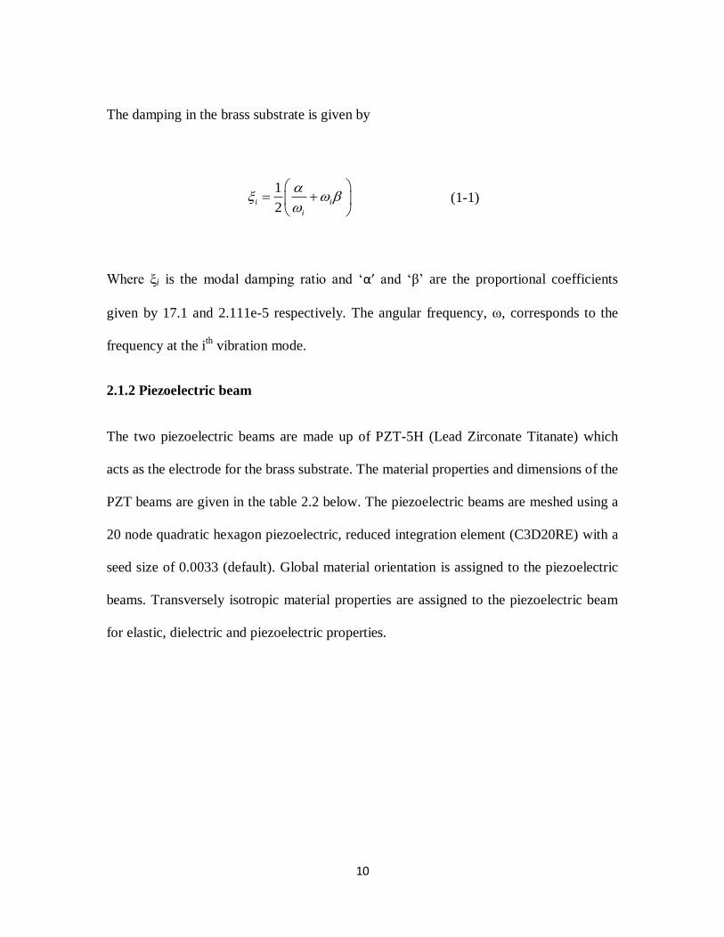
The damping in the brass substrate is given by
1
2i i
i
(1-1)
Where ξi is the modal damping ratio and ‘α’ and ‘β’ are the proportional coefficients
given by 17.1 and 2.111e-5 respectively. The angular frequency, ω, corresponds to the
frequency at the ith vibration mode.
2.1.2 Piezoelectric beam
The two piezoelectric beams are made up of PZT-5H (Lead Zirconate Titanate) which
acts as the electrode for the brass substrate. The material properties and dimensions of the
PZT beams are given in the table 2.2 below. The piezoelectric beams are meshed using a
20 node quadratic hexagon piezoelectric, reduced integration element (C3D20RE) with a
seed size of 0.0033 (default). Global material orientation is assigned to the piezoelectric
beams. Transversely isotropic material properties are assigned to the piezoelectric beam
for elastic, dielectric and piezoelectric properties.

11
Property Value
Density(ρb) 7800 kg/m3
Length (L) 66.62 mm
Width(b) 9.72 mm
Thickness (tb) 0.26 mm
Table 2.2: Properties of the piezoelectric beam
Dielectric Property Value (F/m)
D11 3.89E-08
D22 3.36E-08
D33 3.36E-08
Table 2.3: Dielectric properties of the PZT beam
Elastic Property Value
Uniaxial modulus (c11) 62 GPa
Uniaxial modulus (c22) 62 GPa
Uniaxial modulus (c33) 49 GPa
Shear modulus (c12) 23.5 GPa
Shear modulus (c13) 23 GPa
Shear modulus (c23) 23 GPa
Table 2.4: Elastic properties of the PZT beam

12
Piezoelectric Strain Constants Value (m/V)
d31 -320E-12
d32 -320E-12
d33 -650E-12
Table 2.5: Piezoelectric strain constant of the PZT beam
The constitutive relations of the orthotropic piezoelectric material are explained below.
The relative dielectric constant K3T of PZT-5H is 3800 and the permittivity of free space
is 8.85e-12 F/m. This is used in calculating the dielectric properties in the matrix obtained
in the table 2.3. Table 2.5 shows the transverse isotropic properties of PZT-5H. C11, C22
and C33 are the elastic moduli in the x, y and z, directions.
2.1.3 Derivation of the Constitutive Equations for the Piezoelectric Model
The total charge Q for a continuum volume V with charge density q is defined as:
Q q dV (2-2)
The current density I is defined as the rate of change of total charge Q
I Q (0-3)
The electric field ' is related to the electric potential as
' (0-4)
The total charge accumulated on the boundary of a continuum when it is subjected to an
electric field with volume V is given by

13
dV
Q D n dA (0-5)
Where, D is the electric displacement vector and n is a unit vector normal to the
boundary of the continuum V (i.e. V)
The total electrical potential energy Ue is equal to the work needed to move a total charge
Q in the field and is given by
( )Ue Q (0-6)
Using Maxwell’s equation given by
q divD D (0-7)
And using equation
( ) ( ) ( )D D D (0-8)
Gives,
( )Ue divD dv (0-9)
[ ( ) ]V V
Ue div D dv D dv (0-10)
Applying divergence theorem on the first term of equation (0-10) gives,
[ ]V V
Ue D n dA D dv
(0-11)
14
Neglecting the 1st term (for higher frequency applications, the potential energy and the
electrical displacement decreases with distance), we get,
V
Ue D dv (0-12)
'V
Ue D dv (0-13)
'V
Ue D dv (0-14)
This is the equation for the electrical potential energy of the system.
The total potential energy is the sum of the strain energy and the electrical potential
energy, given by,
[( ) ( ' )]p p i i
V
U S D dv (0-15)
This equation is applicable of standard piezoelectric material in which magnetic effects
and thermal effects are neglected.
The total energy density (energy per unit volume) is given by,
'V p p iU S D (0-16)
'( ) ( )V VV p i
p i
U UU S D
S D
(0-17)
Where the subscripts ‘ε’ and ‘σ’ mean that those values are measured at constant
electrical field (ε=0) and stress (σ=0) respectively.
15
Similarly,
'( ) ( )p p
p q i
q i
S DS D
(0-18)
'
'' ( ) ( )
pii p j
p j
S DS D
(0-19)
Where i,j=1,2,3 and p,q=1,2,3,4,5,6
Also
'( ) ( ) ''
p p
p q i
q i
S SS
(0-20)
'( ) ( ) ''
i ii p j
p j
D DD
(0-20)
From equations (0-18) - (0-21) the linear constitutive equations can be reorganized in the
following form [12]
'D
p pq q pq iS S d (0-21)
' 'i ip p ij jD d (0-22)
Where, S= Mechanical strain, s=Compliance co-efficient matrix (1/spring constant),
d=Piezoelectric strain constant, ε’=Electric field, D=Electric displacement and
= Dielectric constant
In matrix form, these equations can be written as:

16
1 111 12 13 31
2 221 22 23 32
3 331 32 33 33
4 1244 24
44 155 13
11 126 23
0 0 0 0 0
0 0 0 0 0
0 0 0 0 0
0 0 0 0 0 0 0
0 0 0 0 0 0 0
0 0 0 0 0 2( ) 0 0 0
S s s s d
S s s s d
S s s s d
S s d
s dS
s sS
1
2
3
1
2
1 115 11
3
2 24 22 2
12
31 32 33 333 3
13
23
0 0 0 0 0 0 0
0 0 0 0 0 0 0
0 0 0 0 0
D d
D d
d d dD
Alternatively these matrices can also be written in terms of stress matrices
q pq p pq iK S e (0-23)
i ip p ij jD e S (0-24)
Where,
pqK =Stiffness, e=Piezoelectric stress constants
2.1.4 Procedure
The material properties defined above are assigned to the brass and piezoelectric
homogenous solid sections. The sections are then assigned to the individual beams. The
beams are assembled such that the brass substrate is sandwiched between the
piezoelectric beams using translation constraints. The idea is to generate equal potential

17
on the top surface of the top piezoelectric beam (pzt-tt) and the bottom surface of the
bottom piezoelectric beam (pzt-bb). The bottom surface of the top piezoelectric beam
(pzt-tb) and the top surface of the bottom piezoelectric beam (pzt-bt) are kept at a zero
potential. This is achieved by creating node sets for the piezoelectric beams. Two sets,
the master set and the slave set are created for the two ends of the piezoelectric beams
(pzt-tt and pzt-bb). The equation constraint tool is used to implement the constraint on the
electric potential degrees of freedom on these node sets to ensure uniform potential on
these two surfaces of the piezoelectric beams.
The analysis step used for this case is the direct steady state dynamic analysis. The
logarithmic scale is used in this dynamic step and 20 points are generated between the
lower and the upper frequencies. The dynamic step is preceded by a frequency step which
divides the Eigen-frequencies at each frequency range. A symmetric matrix storage
system is used and the Eigen-vectors are normalized by mass. The frequency step
employs a subspace Eigen solver with 18 vectors per iteration and 30 maximum iterations
with 10 Eigen values requested. Non-linear effects on the analysis due to large
deformations are not considered in this analysis.
Field outputs requested in the analysis are the stress and the electric potential. The stress
is calculated at the master node of the piezoelectric beams where the highest stress is
generated. Electric potential can be calculated on any node of the piezoelectric beam,
since it is constrained to be the same across the beam surface. However, for consistency,

18
the electric potential too is calculated at the master node. A tie constraint is used to tie the
brass surfaces to the piezoelectric surfaces (pzt-tb and pzt-bt).
2.1.5 Load
A uniform pressure load of 16Pa was applied along the z direction of the system on top of
the piezoelectric surface (pzt-tt). The load is applied in the dynamic step of the analysis.
The load is applied perpendicular to the piezoelectric beam. The load application is
shown in figure 2.2
Figure 2.2: Loading condition for the solid homogenous substrate beam model
19
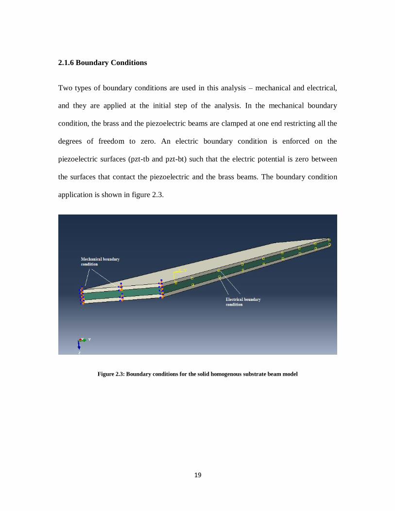
2.1.6 Boundary Conditions
Two types of boundary conditions are used in this analysis – mechanical and electrical,
and they are applied at the initial step of the analysis. In the mechanical boundary
condition, the brass and the piezoelectric beams are clamped at one end restricting all the
degrees of freedom to zero. An electric boundary condition is enforced on the
piezoelectric surfaces (pzt-tb and pzt-bt) such that the electric potential is zero between
the surfaces that contact the piezoelectric and the brass beams. The boundary condition
application is shown in figure 2.3.
Figure 2.3: Boundary conditions for the solid homogenous substrate beam model

20
2.2 Design of the bimorph cantilever honeycomb beam
Similar to the solid plate sandwich structure described above, two more models are
created and analyzed in this thesis. The following section explains the analysis procedure
for the bimorph cantilever beam using two types of honeycomb brass beam as a substrate
sandwiched between two piezoelectric layers. The difference between these two models
and the one described above is that the solid brass substrate plate is replaced by a
honeycomb shell structure (regular and auxetic).
Figure 2.4: Finite element model of the regular honeycomb substrate model

21
Figure 2.5: Finite element model of the auxetic honeycomb substrate model
2.2.1 Effective Properties of the Honeycomb Substrate
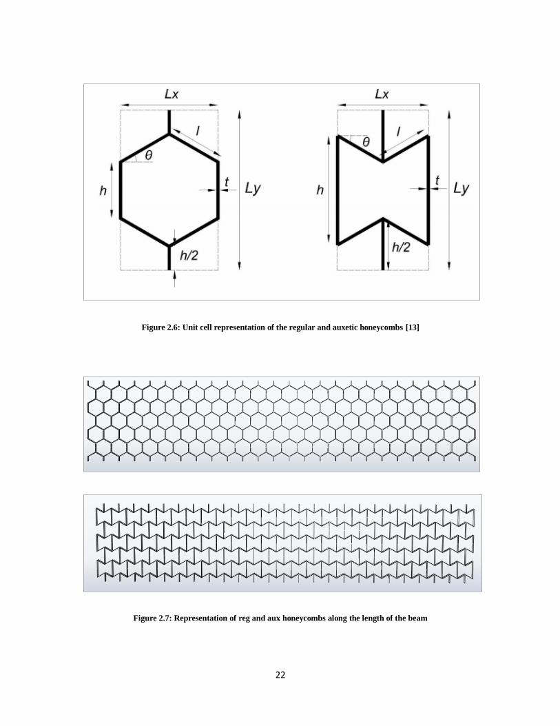
The Finite Element model of the bimorph honeycomb substrate cantilever beam is built
using Abaqus 6.10. The unit cell representation of the regular and the auxetic honeycomb
is shown in figure 2.6. These unit cells are duplicated to form the brass substrate for the
analysis with 25 cells along the length of the substrate and 6 cells along its width.
22
Figure 2.6: Unit cell representation of the regular and auxetic honeycombs [13]
Figure 2.7: Representation of reg and aux honeycombs along the length of the beam
23
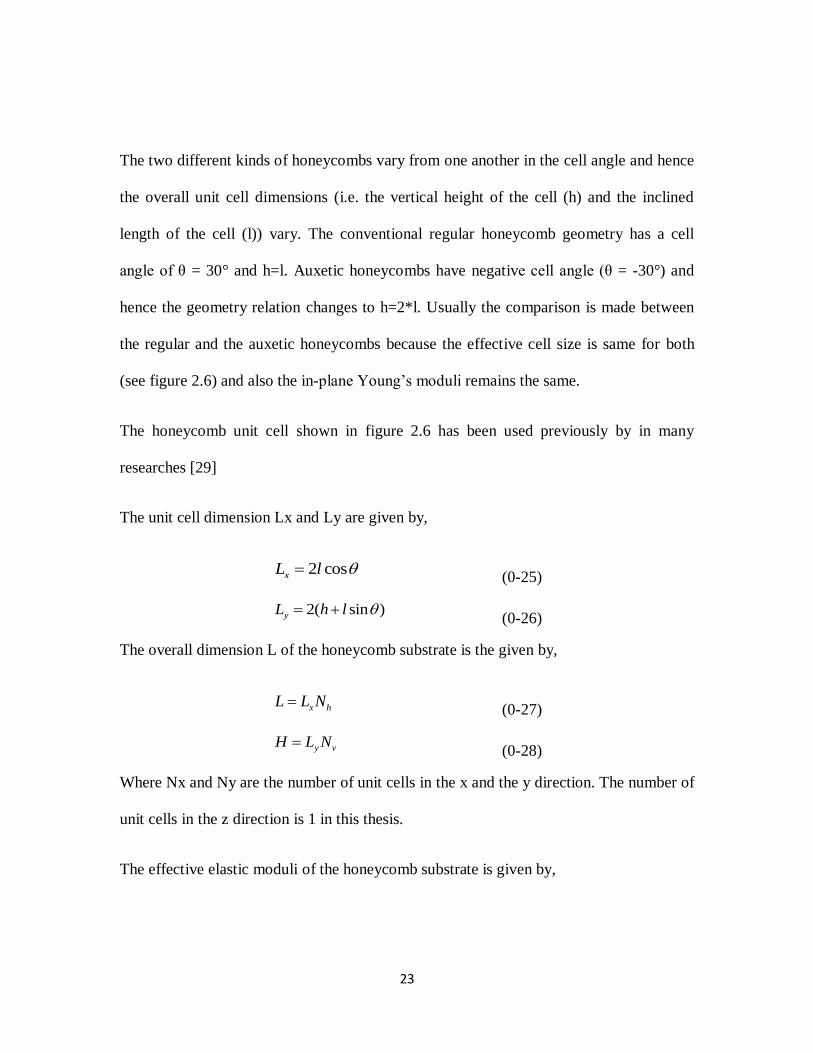
The two different kinds of honeycombs vary from one another in the cell angle and hence
the overall unit cell dimensions (i.e. the vertical height of the cell (h) and the inclined
length of the cell (l)) vary. The conventional regular honeycomb geometry has a cell
angle of θ = 30° and h=l. Auxetic honeycombs have negative cell angle (θ = -30°) and
hence the geometry relation changes to h=2*l. Usually the comparison is made between
the regular and the auxetic honeycombs because the effective cell size is same for both
(see figure 2.6) and also the in-plane Young’s moduli remains the same.
The honeycomb unit cell shown in figure 2.6 has been used previously by in many
researches [29]
The unit cell dimension Lx and Ly are given by,
2 cosxL l (0-25)
2( sin )yL h l (0-26)
The overall dimension L of the honeycomb substrate is the given by,
x hL L N (0-27)
y vH L N (0-28)
Where Nx and Ny are the number of unit cells in the x and the y direction. The number of
unit cells in the z direction is 1 in this thesis.
The effective elastic moduli of the honeycomb substrate is given by,

24
3
*
12
cos
sin sins
t
lE E
h
l
(0-29)
3
*
2 3
sin .
coss
h t
l lE E
(0-30)
*
3
2 .
2 sin coss
h t
l lE E
h
l
(0-31)
Where,
*
1E is the effective in-plane elastic moduli in the x direction,
*
2E is the effective in-plane elastic moduli in the y direction,
*
3E
is the effective out-of-plane elastic moduli in the z direction,
Similarly, the effective shear moduli of the honeycomb substrate is given by,
3
*
12 2
sin .
21 .cos
s
h t
l lG E
h h
l l
(0-32)
*
13
cos .
sins
t
lG G
h
l
(0-33)

25
*
23
sin .
21 .cos
s
h t
l lG G
h
l
(0-34)
Where,
*
12G is the effective in-plane shear moduli, *
13G and *
23G is the effective out-of-plane shear
moduli.
And the effective in-plane effective Poisson’s ratio ( *
12 and *
21 ) is given by,
2
*
12
cos
sin sinh
l
(0-35)
*
21 *
12
1
(0-36)
Note: For the regular honeycomb substrate (θ=30° and h=l) and the auxetic honeycomb
substrate (θ= -30° and h=2*l), the effective in-plane elastic moduli are the same in the x
and y direction are the same and also the effective out-of plane shear moduli are same.
The effective Poisson’s ratio is given by *
12 =1 for the regular honeycomb and *
12 = -1
for the auxetic honeycomb.
The effective density ρ* of the honeycomb core is given by,
*
2 .
2 sin coss
h t
l l
h
l
(0-37)

26
These effective properties are applicable only for the honeycomb substrate. To get the
overall property of the sandwich plate, the properties of the two piezoelectric plates have
to be taken into consideration as well. The mass of the core is given by,
*. . .coreM L H D (0-38)
Where, D is the depth of the core (D=0.76mm for this study).
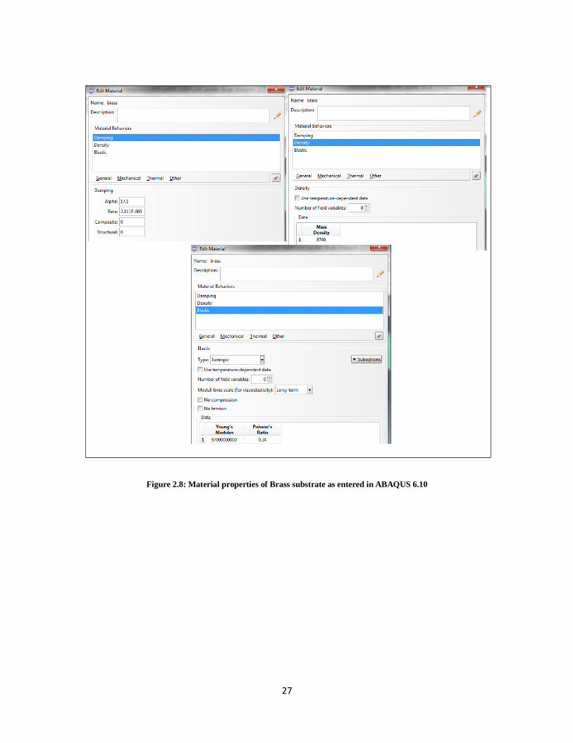
2.2.2 Material properties
The material properties of the piezoelectric beams are the same as defined for the solid
cantilever beam analysis. The piezoelectric beam material is PZT-5H and is assigned
transverse isotropic properties by assigning local material properties. The constitutive
equations of the orthotropic piezoelectric material remain the same as explained in
equations (2-24) and (2-25) where all the variables have the same meaning. The
difference in the material properties arises for the brass substrate where the effective
material properties of the brass hexagonal honeycomb cores are calculated using the
Cellular Material Theory (CMT), to predict the linear elastic behavior of the honeycomb
structures. The material properties entered in ABAQUS 6.10 for brass and the
piezoelectric beams are shown in figure 2.8 and 2.9 below.
27
Figure 2.8: Material properties of Brass substrate as entered in ABAQUS 6.10

28
Figure 2.9 Material properties of Piezoelectric beam as entered in ABAQUS 6.10

29
2.2.3 Analysis Procedure
The finite element analysis for the piezoelectric honeycomb sandwich structure is similar
to the solid plate sandwich structure. The honeycomb brass substrate is made up of 3D
shell extrusion element. It is meshed using reduced integration 8 node doubly curved
thick shelled elements (S8R). The seed size used for meshing the substrate is 0.00036 and
0.00045, which is selected to give 4 and 6 elements across the height for regular and
auxetic honeycomb substrates respectively. The section assigned to the brass honeycomb
substrate is homogenous continuous shell section with a shell thickness of 0.15mm. The
brass substrate is assembled to sandwich between the two piezoelectric plates using edge-
to-edge constraints.

30
Figure 2.10: FEA mesh of the regular honeycomb substrate model
Figure 2.11: FEA mesh of the auxetic honeycomb substrate model
31
The analysis step used for this case is the direct steady state dynamic analysis. The
logarithmic scale is used in this dynamic step and 20 points are generated between the
lower and the upper frequencies. The dynamic step is preceded by a frequency step which
divides the Eigen-frequencies at each frequency range. A symmetric matrix storage
system is used and the Eigen-vectors are normalized by mass. The frequency step
employs a subspace Eigen solver with 18 vectors per iteration and 30 maximum
iterations. 10 Eigen values are requested. Non-linear effects on the analysis due to large
deformations are not considered in this analysis. Field outputs requested in the analysis
are the stress and the electric potential. The stress is calculated at the master node of the
piezoelectric beams where the highest stress is generated. Electric potential can be
calculated on any node of the piezoelectric beam, since it is constrained to be the same
across the beam surface. However, for consistency, the electric potential too is calculated
at the master node. A tie constraint is used to tie the brass surfaces which contact the
piezoelectric surfaces.
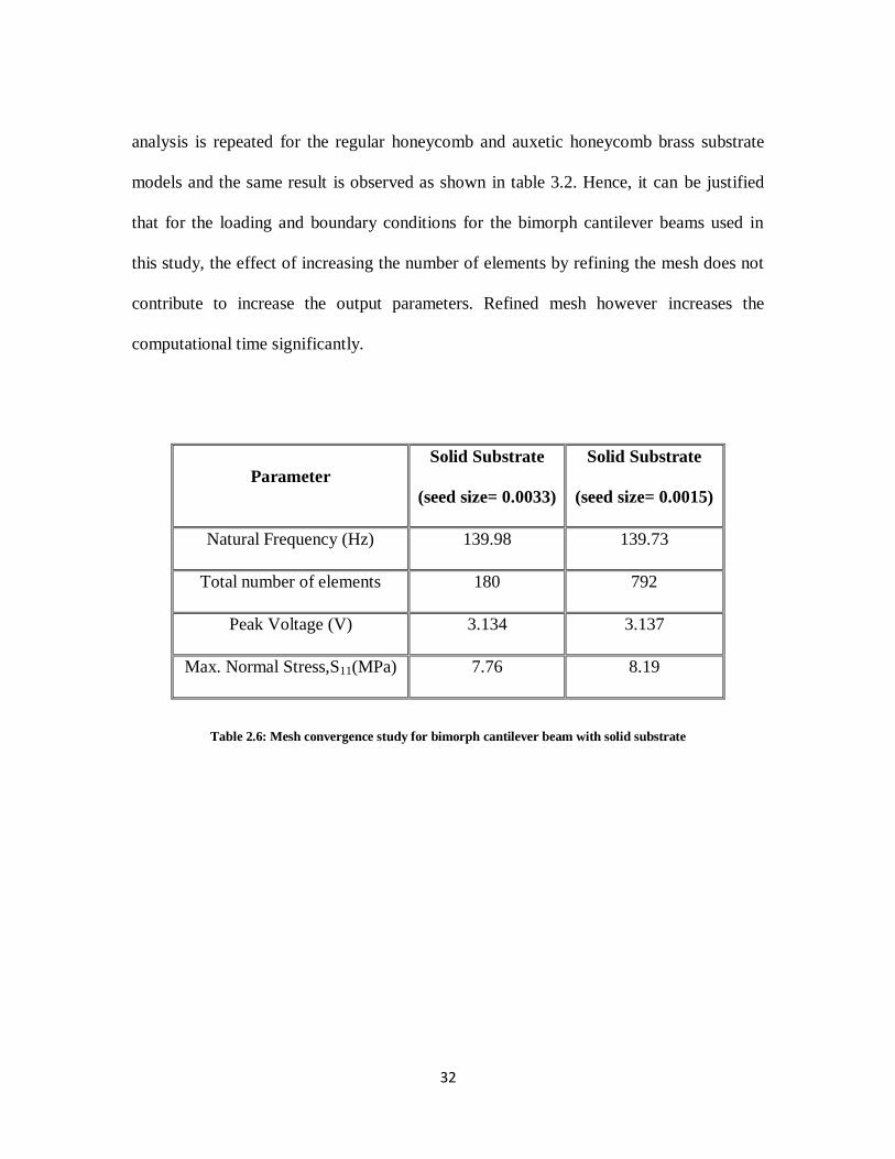
2.2.4 Mesh Convergence Study
A mesh convergence study is done for all three models to study the effect of increasing
the number of elements on the output voltage and stress. The seed sizes for the
homogenous solid substrate and the piezoelectric plate for the bimorph cantilever beam
with solid substrate are reduced to half its previous value. It is observed that reducing the
seed size does not have a significant impact on the output results in this case. Table 3.1
shows the ABAQUS analysis results using reduced seed size for the assembly. The
32
analysis is repeated for the regular honeycomb and auxetic honeycomb brass substrate
models and the same result is observed as shown in table 3.2. Hence, it can be justified
that for the loading and boundary conditions for the bimorph cantilever beams used in
this study, the effect of increasing the number of elements by refining the mesh does not
contribute to increase the output parameters. Refined mesh however increases the
computational time significantly.
Parameter
Solid Substrate
(seed size= 0.0033)
Solid Substrate
(seed size= 0.0015)
Natural Frequency (Hz) 139.98 139.73
Total number of elements 180 792
Peak Voltage (V) 3.134 3.137
Max. Normal Stress,S11(MPa) 7.76 8.19
Table 2.6: Mesh convergence study for bimorph cantilever beam with solid substrate

33
Parameter
Reg HC
Results
(seed size = A)
Reg HC
Results
(seed size = B)
Aux HC
Results
(seed size = C)
Aux HC
Results
(seed size =
D)
Natural
Frequency (Hz)
181.01 180.84 176.57 176.48
Total number
of elements
3776 8746 3788 9682
Peak Voltage
(V)
23.96 23.89 19.21 18.98
Max. Normal
Stress,S11(MPa)
69.15 72.41 55.67 57.74
Table 2.7: Mesh convergence study for bimorph cantilever beam with honeycomb substrate
Seed size A: Brass substrate seed size =0.00036, PZT plate seed size =0.0033
Seed size B: Brass substrate seed size = 0.00025, PZT plate seed size =0.0018
Seed size C: Brass substrate seed size = 0.00045, PZT plate seed size =0.0033
Seed size D: Brass substrate seed size = 0.0003, PZT plate seed size =0.0018
2.2.5 Loading and Boundary Conditions
A uniform pressure load of 16Pa was applied along the z direction of the system on top of
the piezoelectric surface (pzt-tt). The load is applied in the dynamic step of the analysis.

34
The load is applied perpendicular to the piezoelectric beam. Two types of boundary
conditions are used in this analysis – mechanical and electrical, and they are applied at
the initial step of the analysis. In the mechanical boundary condition, the brass and the
piezoelectric beams are clamped at one end restricting all the degrees of freedom to zero.
An electric boundary condition is enforced on the piezoelectric surfaces which are in
contact with the brass surfaces such that the electric potential is zero between the surfaces
that contact them.
2.3 Verification of Abaqus Model
This section provides a validation of the analysis procedure for the Abaqus model used in
this thesis. In this validation model, a cantilever beam consisting of an aluminum
substrate, adhesive layer and a piezoelectric layer (PZT-4) is used with the material
properties given in table 2.8. The procedure of construction of the Abaqus model is
similar to the model creation procedure explained in section 2.1.4. The only difference is
that instead of a mechanical load input given to harness the output voltage, in this case a
constant electrical potential of 12.5kV is applied on the upper surface of piezoelectric
layer, while grounding the lower surface of the piezoelectric layer. The deflection of the
beam due to application of the electrical voltage is calculated and compared to the results
obtained by Saravanos and Heyliger (1995) [40] and Robbins and Reddy (1991) [41].

35
Properties Aluminum Adhesive PZT-4
E11 (GPa) 68.9 6.9 83
E22 (GPa) 68.9 6.9 66
v12 0.25 0.4 0.31
G12 (GPa) 27.6 2.46 -1232
d31 (m/V) 0 0 -1.22E-10
d33 (m/V) 0 0 2.85E-10
ε33 (F/m) 0 0 1.15E-08
ρ (kg/m3) 2769 1662 7.60E+03
Length (m) 0.1524 0.1524 0.1524
Thickness (m) 0.01524 0.01524 0.01524
Width (m) 0.0254 0.0254 0.0254
Table 2.8: Material properties of verification model beams
Figure 2.12: FEA set-up of the verification model
36
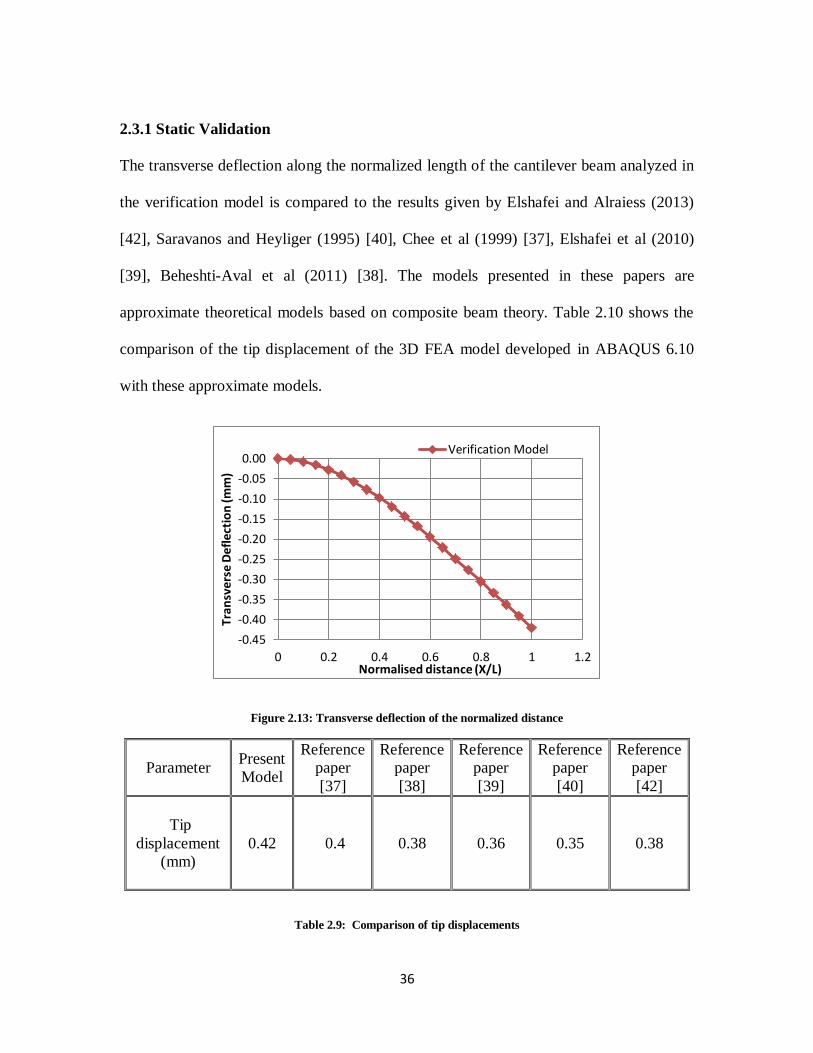
2.3.1 Static Validation
The transverse deflection along the normalized length of the cantilever beam analyzed in
the verification model is compared to the results given by Elshafei and Alraiess (2013)
[42], Saravanos and Heyliger (1995) [40], Chee et al (1999) [37], Elshafei et al (2010)
[39], Beheshti-Aval et al (2011) [38]. The models presented in these papers are
approximate theoretical models based on composite beam theory. Table 2.10 shows the
comparison of the tip displacement of the 3D FEA model developed in ABAQUS 6.10
with these approximate models.
Figure 2.13: Transverse deflection of the normalized distance
Parameter Present
Model
Reference
paper
[37]
Reference
paper
[38]
Reference
paper
[39]
Reference
paper
[40]
Reference
paper
[42]
Tip
displacement
(mm)
0.42 0.4 0.38 0.36 0.35 0.38
Table 2.9: Comparison of tip displacements
-0.45
-0.40
-0.35
-0.30
-0.25
-0.20
-0.15
-0.10
-0.05
0.00
0 0.2 0.4 0.6 0.8 1 1.2
Tra
nsv
erse
Def
lect
ion
(mm
)
Normalised distance (X/L)
Verification Model

37
2.3.2 Dynamic Validation
Table 2.9 shows the fundamental natural frequencies for different number of elements
and is compared to the results given by Elshafei and Alraiess (2013) [42], Robbins and
Reddy (1991) [41] and Saravanos and Heyliger (1995) [40].
Mode No. of
elements
Present
Model
(Hz)
Reference
(a)-(Hz)
Reference
(b)-(Hz)
Reference
(c)-(Hz)
1
10 579.32 470.7 538.4 567.1
20 577.66 470 537.9 544.2
30 577.38 469.9 537.8 544.1
Table 2.10: Fundamental natural frequency comparison
a. Elshafei and Alraiess [42]
b. Robbins and Reddy [41]
c. Saravanos and Heyliger [40]
38
CHAPTER 3: RESULTS OF THE FINITE ELEMENT MODEL
As mentioned in section 2.1.5, the bimorph cantilever beam is given a uniform pressure
load of 16Pa on the top piezoelectric beam surface. This load is selected to compare the
results of the bimorph cantilever solid beam with the two bimorph cantilever honeycomb
beams discussed in the above chapter. In this chapter, the comparison of the results of the
solid beam with the honeycomb beams with a surface pressure of 16Pa is given and the
theory behind calculating these results is explained.
3.1 Basic electrical circuit connection of the bimorph cantilever beam
The analysis model for the bimorph cantilever beam with solid substrate subjected to a
load of 16Pa is divided into two steps, the frequency step and the steady state dynamic
step (henceforth, referred as the dynamic step). The peak value of the electrical potential
is found at the natural frequency at which the beam vibrates. This potential is same along
the surface of the piezoelectric beam due to the equation constraint applied on the master
and slave node sets as explained in the previous chapter. Also, since the two piezoelectric
plates are attached to the solid brass substrate with the contacting surface being at zero
potential, the top surface of the top piezoelectric beam (pzt-tt) – ϕtt and the bottom
surface of the bottom piezoelectric beam (pzt-bb) – ϕbb will be at the same potential. The
output variable given by ABAQUS is the electrical potential. This electrical potential
variable is a complex function and the magnitude of the electrical potential is used for
calculations. The voltages across the two piezoelectric plates is given by,

39
tt bb
tt bb
tt bb
V V V
V – 0 0
V
S
S
S
(3-1)
Where VS is the open source voltage obtained from Abaqus results [12].
As stated earlier, the bimorph cantilever beam essentially symbolizes a capacitor with
brass being the substrate material sandwiched between the two piezoelectric plates. The
capacitance for this is calculated using the following formula:
3 02 T
p
p
LC K b
t
(3-2)
By definition of the basic property of the piezoelectric material, when subjected to a
mechanical load, an electrical potential is generated in the piezoelectric beams due to the
voltage drop across the electrical load. The open source resistance (RS) is a function of
the frequency at different mode intervals (ωi) and the capacitance (Cp) and is calculated
by using the following formula,
1S
i p
RC
(3-3)
where i=1,2…,m
The power harvested and the work done (energy) is a function of the load voltage and
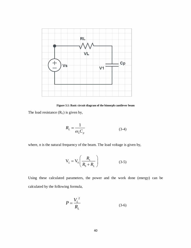
load resistance as seen from the figure 3.1.
40
Figure 3.1: Basic circuit diagram of the bimorph cantilever beam
The load resistance (RL) is given by,
1L
n p
RC
(3-4)
where, n is the natural frequency of the beam. The load voltage is given by,
S
S
V V LL
L
R
R R
(3-5)
Using these calculated parameters, the power and the work done (energy) can be
calculated by the following formula,
2
L
L
VP
R
(3-6)
41
21
2p LW C V (3-7)
3.2 Results and discussion for the FEA Models
The bimorph cantilever solid beam analyzed and discussed above is compared with two
other models (using conventional regular honeycomb and auxetic honeycomb as the
substrate). In this section the results of the comparison models are discussed. For this
comparison, all three models have the same depth for the brass substrates (0.76mm) and
the piezoelectric plates (0.26mm). The load is selected to be 16Pa, as any surface load
higher than this would increase the normal stress of the piezoelectric material beyond
76MPa when regular honeycomb is used a substrate, which in this case is considered as
the failure stress for the piezoelectric material. Hence for an effective comparison, the
limiting stress on the piezoelectric beams is assumed to be 70MPa. The key comparison
results are summarized in the table 3.2 below.

42
Parameter Solid Substrate
Regular HC
Substrate
Auxetic HC
Substrate
Natural Frequency (Hz) 139.974 181.011 176.576
Source Voltage VS (V) 3.13 23.96 19.21
Load Voltage VL (V) 2.21 16.94 13.58
Capacitance (nF) 167.52 22.91 22.91
Core Mass (g) 4.3 0.686 0.918
Total Mass (g) 6.93 4.34 4.59
Load Resistance (KΩ) 6.791 38.41 39.36
Peak Power (mW) 0.72 7.47 4.68
Energy(μJ) 0.409 3.288 2.112
Max. Normal Stress,
S11(MPa)
7.76 69.15 55.67
Table 3.1: Comparison of the finite element analysis results (Load=16Pa)
The peak modal frequency under the first modal vibration mode is found to be 139.974
Hz for the solid beam substrate (henceforth referred as SB). The peak value of the
electrical potential (i.e. the source voltage) found at this natural frequency is 3.13V and
the load voltage is 2.21V. This potential and hence the voltage is the same along the
surface of the piezoelectric beam due to the equation constraint applied on the master and
slave node sets as explained earlier. The peak modal frequency for the regular

43
honeycomb substrate (henceforth referred as RB) and the auxetic honeycomb substrate
(henceforth referred as AB) is found as 181.011Hz and 176.576Hz, respectively. The
electrical potential and hence the source voltage is found to be 23.96V and 19.21V for the
RB and AB, respectively. The load voltage is 16.94V and 13.58V for the RB and AB,
respectively and is compared in the figure 3.3 below.
Figure 3.2: Relation between electrical potential and frequency (Load=16Pa)
0
5
10
15
20
25
30
100 120 140 160 180 200
Ep
ot
(V)
Frequency (Hz)
Solid Substrate
Regular Honeycomb Substrate
Auxetic Honeycomb Substrate

44
Figure 3.3: Relation between load voltage and frequency (Load=16Pa)
The capacitance is calculated using equation (3-2) and is found to be 167.52nF for SB
model and 22.91nF for both RB and AB models. The load resistance which is a function
of the capacitance is calculated from equation (3-3) and is found to be 6.791KΩ,
38.41KΩ and 39.36KΩ for the SB, RB and AB models respectively. By calculating the
resistance and the capacitance, the power and energy can be calculated from equation (3-
6) and (3-7).respectively. The peak power for the SB, RB and AB models are found to be
0.72mW, 7.47mW and 4.68mW respectively. The peak energy generated is 0.41μJ,
3.29μJ and 2.11μJ for the SB, RB and AB models respectively. The peak power and peak
energy generated for the three models is compared in figure 3.9 and 3.10 below.
0
2
4
6
8
10
12
14
16
18
100 120 140 160 180 200
Lo
ad
Vo
ltag
e (V
)
Frequency (Hz)
Solid Substrate
Regular Honeycomb Substrate
Auxetic Honeycomb Substrate

45
Figure 3.4: Relation between power and frequency (Load=16Pa)
Figure 3.5: Relation between energy and frequency (Load=16Pa)
0
1
2
3
4
5
6
7
8
100 120 140 160 180 200
Po
wer
(m
W)
Frequency (Hz)
Solid Substrate
Regular Honeycomb Substrate
Auxetic Honeycomb Substrate
0
0.5
1
1.5
2
2.5
3
3.5
100 120 140 160 180 200
En
ergy (μ
J)
Frequency (Hz)
Solid Substrate
Regular Honeycomb Substrate
Auxetic Honeycomb Substrate

46
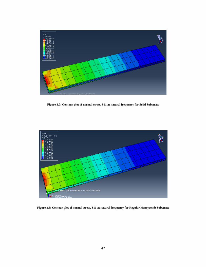
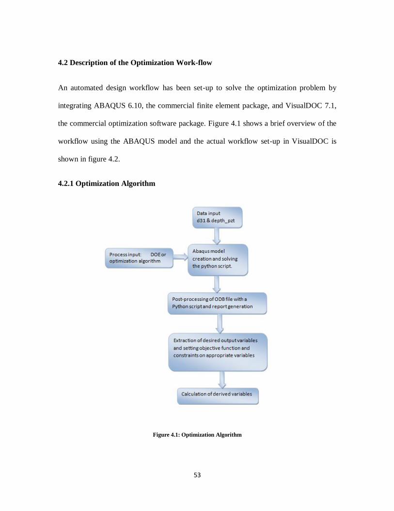
The normal stress components in the x direction, S11 are analyzed and found to be
7.76MPa, 69.15MPa and 55.67MPa at the peak frequency for the SB, RB and the AB
models, respectively. The peak stress is located at the center node of the fixed end of the
beam (Fig 3.7 to Fig 3.9). The contour plot of these stresses is shown in the figure below.
The stress is found to within the limits of the ultimate tensile strength of the piezoelectric
beam (PZT-5H) which is 76MPa [12].
Figure 3.6: Relation between stress and frequency (Load=16Pa)
0
10
20
30
40
50
60
70
80
100 120 140 160 180 200
Str
ess,
S11 (
MP
a)
Frequency (Hz)
Solid Substrate
Regular Honeycomb Substrate
Auxetic Honeycomb Substrate
47
Figure 3.7: Contour plot of normal stress, S11 at natural frequency for Solid Substrate
Figure 3.8: Contour plot of normal stress, S11 at natural frequency for Regular Honeycomb Substrate

48
Figure 3.9: Contour plot of normal stress, S11 at natural frequency for Auxetic Honeycomb Substrate
Parameter
Regular HC/Solid
Substrate
Auxetic HC/Solid
Substrate
Source Voltage VS (V) 7.5 6
Load Voltage VL (V) 7.5 6.5
Stress (MPa) 9 7
Power (μJ) 10.5 6.5
Energy (mW) 8 5
Table 3.2: Summary of FEA models
From the above graphs, it can be seen that using the honeycomb beam substrates result in
higher power generation as compared to the use of solid beam substrates (by a factor of
almost 10). Also the load voltage generated by the honeycomb substrate is nearly 7.5
times more as compared to the solid substrates. The reason for this substantial increase in

49
the voltage generation and thus the power generation is due to the low mass of the
honeycomb structures (as seen from table 3.2) which allows the beam to vibrate at a
higher frequency and amplitude which eventually results in more voltage generation for a
given load.

50
CHAPTER 4: ENGINEERING OPTIMIZATION PROBLEM
The dimensions and the material properties of the piezoelectric beams used in the finite
element models explained in the previous chapters are selected based on the
specifications given by the manufacturer. The objective of using the bimorph cantilever
beams is to maximize the output voltage for a given pressure load. The input parameters
are the dimensions and material properties for the beams and the constraint, in this case,
is the ultimate tensile strength of the piezoelectric beam. However, the efficiency of these
models can be increased by optimizing the input parameters for the same loading
conditions and constraints, to give better desired output which is the voltage generated. In
this chapter, the engineering optimization problem set-up details are explained.
4.1 Optimization Problem
4.1.1 Objective Statement
The objective of the optimization problem is to maximize the energy harvested (i.e.
voltage output) for the bimorph solid and honeycomb beam models. The multi-physics
problem selected is subjected to two input parameter limiting conditions – the depth of
the piezoelectric beam (depthpzt) and the piezoelectric strain constant in x direction (d31).
The constraint is the Ultimate Tensile strength of the piezoelectric beam. The
optimization tool used for this thesis is VisualDOC 7.1.

51
4.1.2 Input Parameters
The input parameters for the optimization problem are listed in table 4.1. In order to
define the design space of the problem, the upper and lower limits of each parameter is
listed. To verify that the convergence of the optimization model is not constrained due to
the parameter limits, the solid brass substrate model is optimized with a wider range limit
(table 4.2) on the parameters and the optimized output variables are calculated.
Variables Lower Limit Upper Limit
Depthpzt (mm) 0.13 0.39
d31 (m/V) -4.8E-10 -1.6E-10
Table 4.1: Limits for the optimization input variables
Variables Lower Limit Upper Limit
Depthpzt (mm) 0.065 0.459
d31 (m/V) -6E-10 -1E-10
Table 4.2: Limits for the optimization input variables for convergence verification
4.1.3 Output Parameters
The output variable for the optimization problem is the voltage generated by the beam
under the given loading conditions. This output variable has been chosen to obtain a
single representative value of the energy harvesting performance of the sandwich plate
for the chosen frequency range since the voltage varies according to the frequency, the

52
time and the position. The value obtained is the maximum voltage generated at the
resonant frequency.
4.1.4 Derived Variables
The primary output variable from the optimization process is the source voltage (Epot)
generated at the surface of the piezoelectric plates for given range of frequencies.
Other variables such as resistance, load voltage, power and energy are calculated as
explained in section 3.1.
4.1.5 Constraints
Any design must resist the dynamic load and be reliable. It is constrained such that the
maximum stress is less than ultimate tensile strength. So for these reasons we choose of
the ultimate tensile strength as an admissible stress as the problem has linear elastic
properties.
7 27.6 [ / ]a E N m
Mathematically, the objective statement can be written as,
Maximize: Source Voltage, Vs (tp, d31)
Subject to: 0.13 (mm) ≤ tp ≤ 0.39 (mm);
-4.8E-10 (m/V) ≤ d31 ≤ -1.6E-10 (m/V)
7 27.6 [ / ]a E N m
53
4.2 Description of the Optimization Work-flow
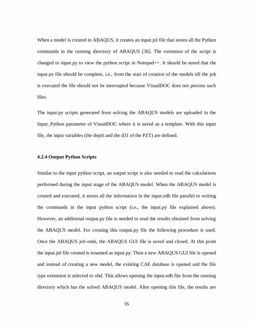
An automated design workflow has been set-up to solve the optimization problem by
integrating ABAQUS 6.10, the commercial finite element package, and VisualDOC 7.1,
the commercial optimization software package. Figure 4.1 shows a brief overview of the
workflow using the ABAQUS model and the actual workflow set-up in VisualDOC is
shown in figure 4.2.
4.2.1 Optimization Algorithm
Figure 4.1: Optimization Algorithm

54
4.2.2 VisualDOC Worflow
Figure 4.2: Optimization Workflow
4.2.3 Input Python Scripts
The VisualDOC workflow shown above is a controlled loop algorithm which starts with
the input Python language script, which is a file containing the different steps to generate
the 3D model for the bimorph piezoelectric beam model. The list of commands to write
the code is available in the “Scripting Reference Manual” of ABAQUS documentation
[36]. This script takes into account various input parameters like the dimensions of the
beams, material properties, the constraint equations, etc. and solves the model. A detailed
list of the files for all three models as well as the reference solid substrate model is given
in table 4.2 and a sample file is attached in the appendix section (A).
55
When a model is created in ABAQUS, it creates an input.jnl file that stores all the Python
commands in the running directory of ABAQUS [36]. The extension of the script is
changed to input.py to view the python script in Notepad++. It should be noted that the
input.py file should be complete, i.e., from the start of creation of the models till the job
is executed the file should not be interrupted because VisualDOC does not process such
files.
The input.py scripts generated from solving the ABAQUS models are uploaded in the
Input_Python parameter of VisualDOC where it is saved as a template. With this input
file, the input variables (the depth and the d31 of the PZT) are defined.
4.2.4 Output Python Scripts
Similar to the input python script, an output script is also needed to read the calculations
performed during the input stage of the ABAQUS model. When the ABAQUS model is
created and executed, it stores all the information in the input.odb file parallel to writing
the commands in the input python script (i.e., the input.py file explained above).
However, an additional output.py file is needed to read the results obtained from solving
the ABAQUS model. For creating this output.py file the following procedure is used.
Once the ABAQUS job ends, the ABAQUS GUI file is saved and closed. At this point
the input.jnl file created is renamed as input.py. Then a new ABAQUS GUI file is opened
and instead of creating a new model, the existing CAE database is opened and the file
type extension is selected to obd. This allows opening the input.odb file from the running
directory which has the solved ABAQUS model. After opening this file, the results are

56
viewed and stored in a report file (result.rpt) and the ABAQUS GUI is saved and closed.
The running directory at this stage creates a file called abaqus.rpy which is renamed to
output.py, which can again be edited in Notepad++.
Similar to the input scripts, the output python scripts generated from solving the
ABAQUS models are uploaded in the Output_Python parameter of VisualDOC where it
is saved as a template. This file, however, does not need any variables to be defined.
4.2.5 Challenges in integrating VisualDOC 7.1 and ABAQUS 6.10
The important points to note when integrating the two softwares are:
The scripts must generate the desired ABAQUS models, outputs and reports
without errors and interruptions.
The directory path of the outputs and reports should be removed from the output
scripts.
4.2.5.1 Location of the output files generated by ABAQUS
By default ABAQUS generates the output files i.e., the “.odb” and “.rpt” files in the
“C:\Temp” folder of the machine. However for VisualDOC 7.1 to read and process these
files they must be saved to its running directory which is different than “C:\Temp”.
Hence the python scripts have to be altered to accommodate these changes. Also, the
directory path of the outputs and reports should be removed from the output scripts.

57
4.2.5.2 Compatibility of the versions of the softwares
VisualDOC 7.1 is compatible with ABAQUS 6.10 and lower versions. In this thesis,
VisualDOC 7.1 is used with ABAQUS 6.10.
Note: The file names mentioned in section 4.1.3 and 4.1.4 are for explanation purposes
only. The detailed file names of the three bimorph piezoelectric models are given in table
4.2 below.
Parameter Solid Brass substrate model
Input_Python solid-parallel-16.py
Run_Abaqus_In run-solid16.bat
Output_Python abaqus-solid16.py
Run_Abaqus_Out pp-solid16.bat
`Parameter Reg HC Brass substrate model
Input_Python reghc-parallel-optimiz.py
Run_Abaqus_In runabaqus-reghc-parallel.bat
Output_Python abaqus-reghc-parallel.py
Run_Abaqus_Out postprocessing-reghc-parallel.bat
Parameter Aux HC Brass substrate model
Input_Python auxhc-parallel-optim.py
Run_Abaqus_In runabaqus-auxhc-parallel.bat
Output_Python abaqus-auxhc-parallel.py
Run_Abaqus_Out postprocessing-auxhc-parallel.bat
Table 4.3: VisualDOC input file names

58
4.2.6 Executable parameters
The Run_Abaqus_In and the Run_Abaqus_Out are executable components used to run
the analysis in the optimization model. The Run_Abaqus_In reads the input python script
from the Input_Python parameter does the computation and creates the results which are
stored in the Out_Python parameter. This is then used as input for another executable
parameter Run_Abaqus_Out to read and execute the output python script and store the
results in the Report parameter. Since the executable component is designed to run an
external analysis program, no data editor is provided for the executable component. The
executable files are capable of reading and computing the uploaded python scripts
provided the name of the interpreter is provided as the name of the analysis program and
the script file as an argument.
4.2.7 Report
The report file (report.rpt) contains the information of the analysis of the model.
VisualDOC saves the report as a template and the objectives, constraints or variables
needed are extracted. In this case the parameters extracted are the maximum stress and
maximum electrical potential obtained from the analysis.
4.3 Optimization
The optimization component supports two types of algorithms, the Gradient based
optimization and the Non-Gradient based optimization. For this thesis, the Non Gradient
optimization component is selected.

59
4.3.1 Non-Gradient Based Optimization
The non-gradient based optimization is used as the objective function is discontinuous
with respect to the input parameters. Such algorithms are primarily based on heuristic
search principles and are non-deterministic in nature.
4.3.2 Non-dominated Sorting Genetic Algorithm II
The NSGA-II algorithm is used to perform non-gradient based optimization. This
algorithm works for continuous, discrete, and integer variable problems. It performs
global optimization by enforcing the constraint limits and is usually very robust.
4.3.3 Starting and Stopping criteria
The starting criterion used is random which allows the user to create a random set of
initial points. The initial population size of 5 is used for this problem. The Stopping
Criteria is used to determine when to terminate the optimization process. For this problem
a maximum of 20 iterations is used. The population size and the number of iterations are
selected after running a few iterations (not covered in this thesis) with different
combinations of these values. It was found that these numbers are sufficient for
convergence and can be generalized for all the models included in the study. The
optimization will be forced to terminate if the maximum number of iterations is reached
and convergence is assumed if any of the specified convergence criteria are met.
For every loop of the algorithm, the input and output ABAQUS python scripts are
executed five times per iterations with a maximum number of twenty iterations. In other
60
words, a design of experiments with five designs of random combinations of the input
parameters from the given limit range is set up per iteration. At the end of each iteration,
the NSGA-II algorithm generates a best solution set which is the most significant set of
input and output parameters from the DOE set-up for a given iteration. The best solution
set generated at the last iteration is the optimum value as there in no further change in the
parameter when the iterations are increased.
4.3.4 GA Parameter
• Probability of Crossover
This sets the probability of performing crossover when generating a new offspring.
Typically this should be 1.0 or a value close to 1.0. In NSGA-II, the simulated binary
cross over is used to generate new offsprings. In this thesis the probability of crossover is
selected as 0.8.
• DisIndex for Crossover
Distribution index is a parameter that defines the shape of the probability distribution for
the crossover operator. For small values, points far away from the parents are likely to be
generated, whereas for large values, points closer to the parents are likely to be generated.
The distribution index for crossover selected in this thesis is 10 which is the default
value.
61
• Probability of Mutation
Mutation is used to introduce additional randomness into the design to avoid premature
convergence. The probability of mutation should be as typically in the range of 0.1 to 0.2.
In this thesis, the probability of mutation is 0.1, which is the default value in VisualDoc
7.1.
• DisIndex for Mutation
Distribution index is a parameter that defines the shape of the probability distribution for
mutation operator. For small values, points far away from the original point are likely to
be generated, whereas for large values, points closer to the original point are likely to be
generated. The distribution index for mutation selected in this thesis is 15 which is the
default value.
4.4 Data Linker
Data linking is essentially joining all the building blocks of the VisualDOC flowchart in
the workflow by linking the data and the parameters of different parameters together. The
links are the basic means of information transfer between the pair of components. The
data flow for the optimization component is shown in the figure below. By linking the
data in the data linker, an optimization link table is generated which allows to define the
problem domain. In the link table, the input, output and the constraints are set as required.

62
Figure 4.3: Data linking in VisualDOC [37]
4.5 Simulation Monitors
The simulation monitors are used to simulate the progress of the optimization in real
time. For this study, four simulation monitors are set-up: Depth and d31 vs the number of
iterations as the monitors for the input variables and E-pot and Stress vs the number of
iterations as the monitors for the output variables. The x-axis is defined as the number of
iterations which gives the best solution set for every population iterated. This is done to
avoid the accumulation of data points generated from all the populations iterated and
gives only the ‘best’ results for every population.
63
CHAPTER 5: ANALYSIS OF THE OPTIMIZATION MODEL
RESULTS
5.1 Results of the Optimization model
The NSGA-II algorithm in the optimization model generates a set of best solution set at
every iteration. For initial iterations, the algorithm executes the ABAQUS model for the
given population size and generates random values for the input parameters within the
given limits. With these five set of values as the input parameters, the ABAQUS model is
executed and the output values along with the constraints is found. The best solution set
values for the given iteration is the set of input values which gives the maximum output
within the constraint limit. The same procedure is repeated and the best solution sets are
reported for every iteration. It is observed that after a few iterations, the optimization
converges and stabilizes as the best solution set remains almost constant. If the maximum
output calculated for a given iteration is less than that found in the preceding iteration,
then the solution set with higher value is reported.
The graphs below show the history of the optimization. The first population of the first
iteration starts with the initially entered input values. At this point, the algorithm iterates
within the limits of the input values to solve the ABAQUS model and finds the maximum
which is reported as the first best solution set. The range of variation of the input
variables to find the maximum reduces with every iteration as the algorithm gets a fair
idea of where the optimum can be located.
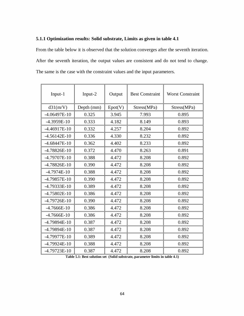
64
5.1.1 Optimization results: Solid substrate, Limits as given in table 4.1
From the table below it is observed that the solution converges after the seventh iteration.
After the seventh iteration, the output values are consistent and do not tend to change.
The same is the case with the constraint values and the input parameters.
Input-1 Input-2 Output Best Constraint Worst Constraint
d31(m/V) Depth (mm) Epot(V) Stress(MPa) Stress(MPa)
-4.06497E-10 0.325 3.945 7.993 0.895
-4.3959E-10 0.333 4.182 8.149 0.893
-4.46917E-10 0.332 4.257 8.204 0.892
-4.56142E-10 0.336 4.330 8.232 0.892
-4.68447E-10 0.362 4.402 8.233 0.892
-4.78826E-10 0.372 4.470 8.263 0.891
-4.79707E-10 0.388 4.472 8.208 0.892
-4.78826E-10 0.390 4.472 8.208 0.892
-4.7974E-10 0.388 4.472 8.208 0.892
-4.79857E-10 0.390 4.472 8.208 0.892
-4.79333E-10 0.389 4.472 8.208 0.892
-4.75802E-10 0.386 4.472 8.208 0.892
-4.79726E-10 0.390 4.472 8.208 0.892
-4.7666E-10 0.386 4.472 8.208 0.892
-4.7666E-10 0.386 4.472 8.208 0.892
-4.79894E-10 0.387 4.472 8.208 0.892
-4.79894E-10 0.387 4.472 8.208 0.892
-4.79977E-10 0.389 4.472 8.208 0.892
-4.79924E-10 0.388 4.472 8.208 0.892
-4.79723E-10 0.387 4.472 8.208 0.892
Table 5.1: Best solution set (Solid substrate, parameter limits in table 4.1)
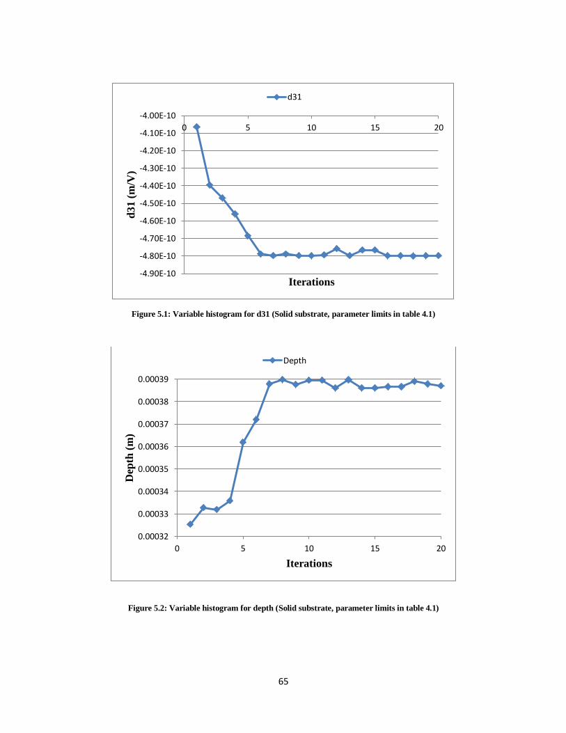
65
Figure 5.1: Variable histogram for d31 (Solid substrate, parameter limits in table 4.1)
Figure 5.2: Variable histogram for depth (Solid substrate, parameter limits in table 4.1)
-4.90E-10
-4.80E-10
-4.70E-10
-4.60E-10
-4.50E-10
-4.40E-10
-4.30E-10
-4.20E-10
-4.10E-10
-4.00E-10
0 5 10 15 20d
31
(m
/V)
Iterations
d31
0.00032
0.00033
0.00034
0.00035
0.00036
0.00037
0.00038
0.00039
0 5 10 15 20
Dep
th (
m)
Iterations
Depth

66
Figure 5.3: Variable histogram for E-pot (Solid substrate, parameter limits in table 4.1)
Figure 5.4: Variable histogram for stress (Solid substrate, parameter limits in table 4.1)
3.9
4
4.1
4.2
4.3
4.4
4.5
0 5 10 15 20
Ep
ot(
V)
Iterations
Epot
7.9
7.95
8
8.05
8.1
8.15
8.2
8.25
8.3
0 5 10 15 20
Str
ess(
MP
a)
Iterations
Stress
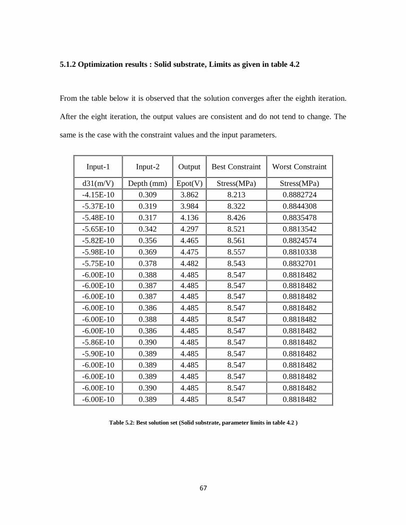
67
5.1.2 Optimization results : Solid substrate, Limits as given in table 4.2
From the table below it is observed that the solution converges after the eighth iteration.
After the eight iteration, the output values are consistent and do not tend to change. The
same is the case with the constraint values and the input parameters.
Input-1 Input-2 Output Best Constraint Worst Constraint
d31(m/V) Depth (mm) Epot(V) Stress(MPa) Stress(MPa)
-4.15E-10 0.309 3.862 8.213 0.8882724
-5.37E-10 0.319 3.984 8.322 0.8844308
-5.48E-10 0.317 4.136 8.426 0.8835478
-5.65E-10 0.342 4.297 8.521 0.8813542
-5.82E-10 0.356 4.465 8.561 0.8824574
-5.98E-10 0.369 4.475 8.557 0.8810338
-5.75E-10 0.378 4.482 8.543 0.8832701
-6.00E-10 0.388 4.485 8.547 0.8818482
-6.00E-10 0.387 4.485 8.547 0.8818482
-6.00E-10 0.387 4.485 8.547 0.8818482
-6.00E-10 0.386 4.485 8.547 0.8818482
-6.00E-10 0.388 4.485 8.547 0.8818482
-6.00E-10 0.386 4.485 8.547 0.8818482
-5.86E-10 0.390 4.485 8.547 0.8818482
-5.90E-10 0.389 4.485 8.547 0.8818482
-6.00E-10 0.389 4.485 8.547 0.8818482
-6.00E-10 0.389 4.485 8.547 0.8818482
-6.00E-10 0.390 4.485 8.547 0.8818482
-6.00E-10 0.389 4.485 8.547 0.8818482
Table 5.2: Best solution set (Solid substrate, parameter limits in table 4.2 )
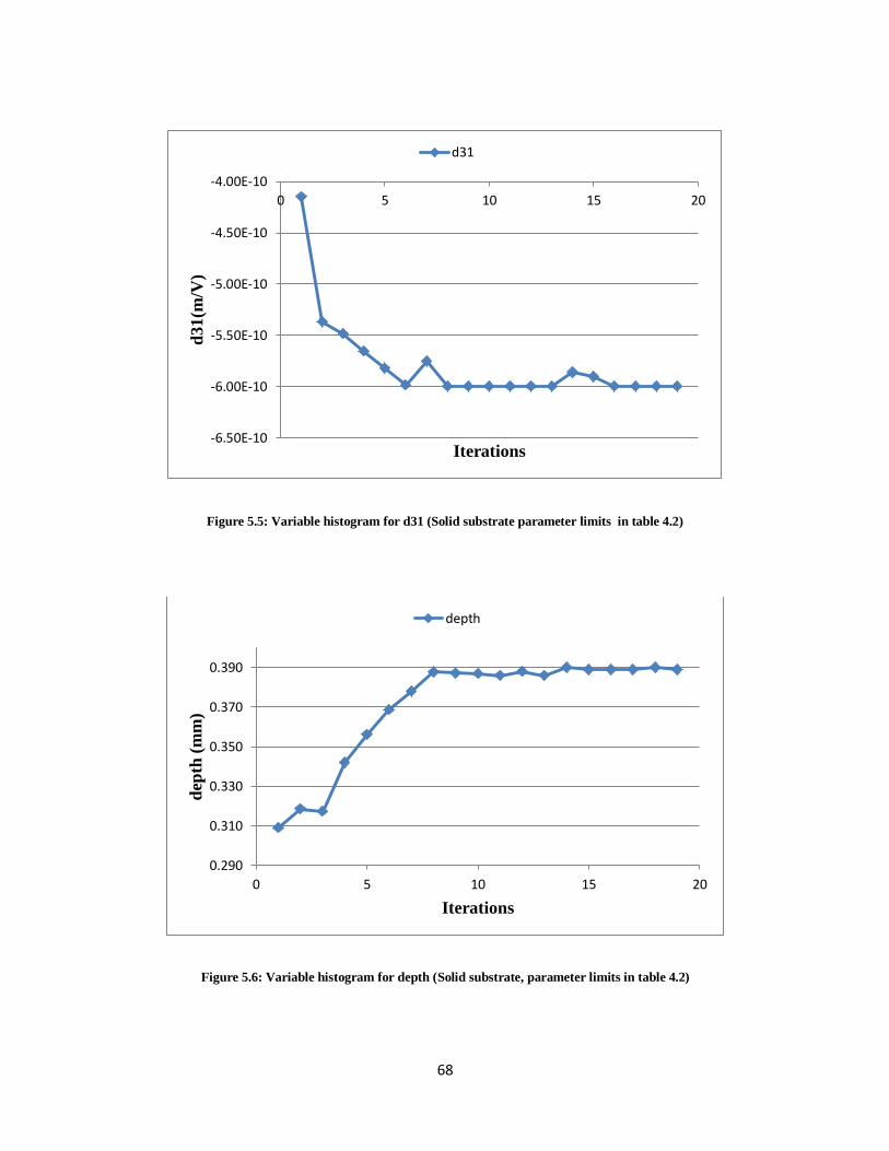
68
Figure 5.5: Variable histogram for d31 (Solid substrate parameter limits in table 4.2)
Figure 5.6: Variable histogram for depth (Solid substrate, parameter limits in table 4.2)
-6.50E-10
-6.00E-10
-5.50E-10
-5.00E-10
-4.50E-10
-4.00E-10
0 5 10 15 20d
31
(m/V
)
Iterations
d31
0.290
0.310
0.330
0.350
0.370
0.390
0 5 10 15 20
dep
th (
mm
)
Iterations
depth

69
Figure 5.7: Variable histogram for E-pot (Solid substrate, parameter limits in table 4.2)
Figure 5.8: Variable histogram for stress (Solid substrate, parameter limits in table 4.2)
3.75
3.85
3.95
4.05
4.15
4.25
4.35
4.45
4.55
0 5 10 15 20
Ep
ot
(V)
Iterations
Epot
8.200
8.250
8.300
8.350
8.400
8.450
8.500
8.550
8.600
0 5 10 15 20
Str
ess
(MP
a)
Iterations
Stress
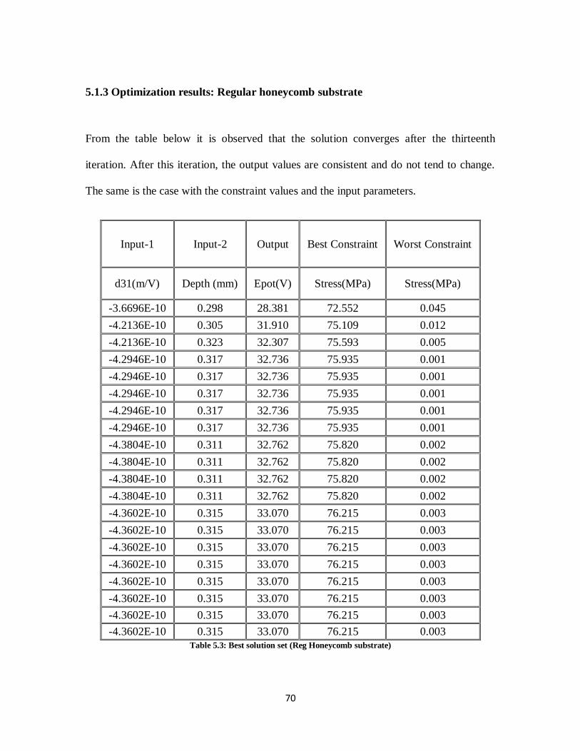
70
5.1.3 Optimization results: Regular honeycomb substrate
From the table below it is observed that the solution converges after the thirteenth
iteration. After this iteration, the output values are consistent and do not tend to change.
The same is the case with the constraint values and the input parameters.
Input-1 Input-2 Output Best Constraint Worst Constraint
d31(m/V) Depth (mm) Epot(V) Stress(MPa) Stress(MPa)
-3.6696E-10 0.298 28.381 72.552 0.045
-4.2136E-10 0.305 31.910 75.109 0.012
-4.2136E-10 0.323 32.307 75.593 0.005
-4.2946E-10 0.317 32.736 75.935 0.001
-4.2946E-10 0.317 32.736 75.935 0.001
-4.2946E-10 0.317 32.736 75.935 0.001
-4.2946E-10 0.317 32.736 75.935 0.001
-4.2946E-10 0.317 32.736 75.935 0.001
-4.3804E-10 0.311 32.762 75.820 0.002
-4.3804E-10 0.311 32.762 75.820 0.002
-4.3804E-10 0.311 32.762 75.820 0.002
-4.3804E-10 0.311 32.762 75.820 0.002
-4.3602E-10 0.315 33.070 76.215 0.003
-4.3602E-10 0.315 33.070 76.215 0.003
-4.3602E-10 0.315 33.070 76.215 0.003
-4.3602E-10 0.315 33.070 76.215 0.003
-4.3602E-10 0.315 33.070 76.215 0.003
-4.3602E-10 0.315 33.070 76.215 0.003
-4.3602E-10 0.315 33.070 76.215 0.003
-4.3602E-10 0.315 33.070 76.215 0.003
Table 5.3: Best solution set (Reg Honeycomb substrate)
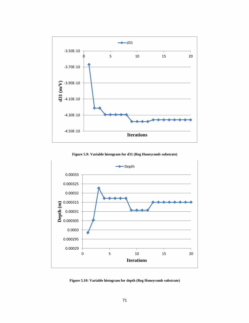
71
Figure 5.9: Variable histogram for d31 (Reg Honeycomb substrate)
Figure 5.10: Variable histogram for depth (Reg Honeycomb substrate)
-4.50E-10
-4.30E-10
-4.10E-10
-3.90E-10
-3.70E-10
-3.50E-10
0 5 10 15 20d
31 (
m/V
)
Iterations
d31
0.00029
0.000295
0.0003
0.000305
0.00031
0.000315
0.00032
0.000325
0.00033
0 5 10 15 20
Dep
th (
m)
Iterations
Depth

72
Figure 5.11: Variable histogram for electrical potential (Reg Honeycomb substrate)
Figure 5.12: Variable histogram for stress (Reg Honeycomb substrate)
28
29
30
31
32
33
34
0 5 10 15 20
Ep
ot
(V)
Iterations
Epot
72
72.5
73
73.5
74
74.5
75
75.5
76
76.5
0 5 10 15 20
Str
ess
(MP
a)
Iterations
Stress
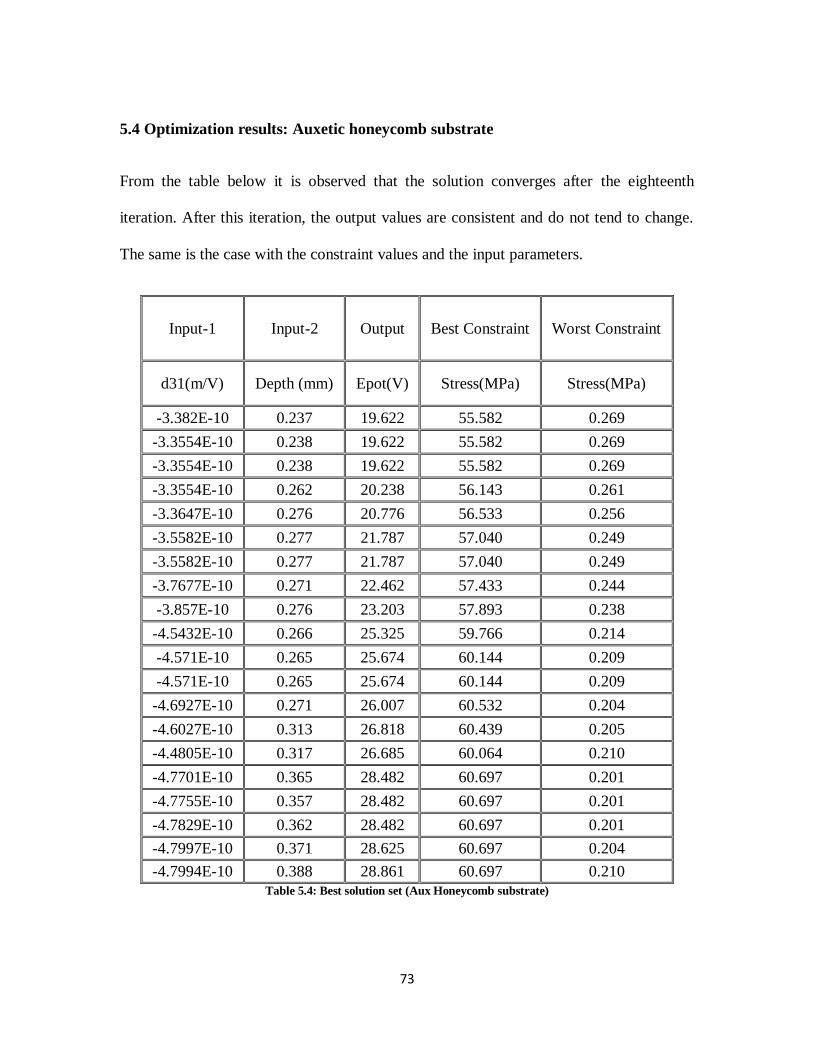
73
5.4 Optimization results: Auxetic honeycomb substrate
From the table below it is observed that the solution converges after the eighteenth
iteration. After this iteration, the output values are consistent and do not tend to change.
The same is the case with the constraint values and the input parameters.
Input-1 Input-2 Output Best Constraint Worst Constraint
d31(m/V) Depth (mm) Epot(V) Stress(MPa) Stress(MPa)
-3.382E-10 0.237 19.622 55.582 0.269
-3.3554E-10 0.238 19.622 55.582 0.269
-3.3554E-10 0.238 19.622 55.582 0.269
-3.3554E-10 0.262 20.238 56.143 0.261
-3.3647E-10 0.276 20.776 56.533 0.256
-3.5582E-10 0.277 21.787 57.040 0.249
-3.5582E-10 0.277 21.787 57.040 0.249
-3.7677E-10 0.271 22.462 57.433 0.244
-3.857E-10 0.276 23.203 57.893 0.238
-4.5432E-10 0.266 25.325 59.766 0.214
-4.571E-10 0.265 25.674 60.144 0.209
-4.571E-10 0.265 25.674 60.144 0.209
-4.6927E-10 0.271 26.007 60.532 0.204
-4.6027E-10 0.313 26.818 60.439 0.205
-4.4805E-10 0.317 26.685 60.064 0.210
-4.7701E-10 0.365 28.482 60.697 0.201
-4.7755E-10 0.357 28.482 60.697 0.201
-4.7829E-10 0.362 28.482 60.697 0.201
-4.7997E-10 0.371 28.625 60.697 0.204
-4.7994E-10 0.388 28.861 60.697 0.210
Table 5.4: Best solution set (Aux Honeycomb substrate)

74
Figure 5.13: Variable histogram for d31 (Aux Honeycomb substrate)
Figure 5.14: Variable histogram for depth (Aux Honeycomb substrate)
-5.00E-10
-4.80E-10
-4.60E-10
-4.40E-10
-4.20E-10
-4.00E-10
-3.80E-10
-3.60E-10
-3.40E-10
-3.20E-10
0 5 10 15 20d
31
(m
/V)
Iterations
d31
0.000235
0.000255
0.000275
0.000295
0.000315
0.000335
0.000355
0.000375
0.000395
0 5 10 15 20
Dep
th (
m)
Iterations
Depth

75
Figure 5.15: Variable histogram for electrical potential (Aux Honeycomb substrate)
Figure 5.16: Variable histogram for stress (Aux Honeycomb substrate)
19.6
20.6
21.6
22.6
23.6
24.6
25.6
26.6
27.6
28.6
0 5 10 15 20
Ep
ot
(V)
Iterations
Epot
55.5
56.5
57.5
58.5
59.5
60.5
0 5 10 15 20
Str
ess
(MP
a)
Iterations
Stress

76
Note: The maximum stress value for the solid substrate models is less than the constraint
stress because of the limits given for the input parameters. These limits are selected to
maintain consistency across all the four models analyzed such that the optimized stress
does not exceed the constraint limit for any of these models. Also from the tables above,
it is observed that the optimized value of d31 tends towards the upper limit value.
5.2 Verification of the optimization results & comparison of the ABAQUS models
The ABAQUS models are executed with the optimized values obtained in section 5.1 as
the input parameters to verify the output results of VisualDOC. The results are shown in
table 5.5. It is observed that for the same input parameters, there is a variation in the
output parameters. The reason for this variation is that VisualDOC optimizes only two
parameters of the ABAQUS model. However, the output of the ABAQUS depends on all
the material and geometric parameters of both the substrate and the piezoelectric beams.
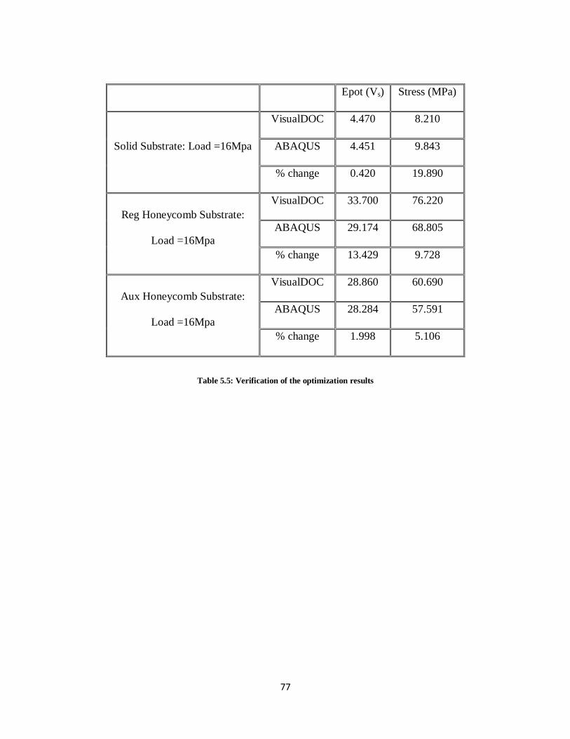
77
Epot (Vs) Stress (MPa)
Solid Substrate: Load =16Mpa
VisualDOC 4.470 8.210
ABAQUS 4.451 9.843
% change 0.420 19.890
Reg Honeycomb Substrate:
Load =16Mpa
VisualDOC 33.700 76.220
ABAQUS 29.174 68.805
% change 13.429 9.728
Aux Honeycomb Substrate:
Load =16Mpa
VisualDOC 28.860 60.690
ABAQUS 28.284 57.591
% change 1.998 5.106
Table 5.5: Verification of the optimization results

78
Solid Substrate: Load = 16MPa
Parameters Before After %
change
Input Parameters
Depth of PZT (mm) - tp 0.260 0.387 48.846
Width of PZT (m) - b 0.010 0.010 0
Length of PZT (m) - L 0.067 0.067 0
Piezoelectric Relative Dielectric Constant -
K3t 3800 3800 0
Permittivity of Free space (F/m) 8.85E-12 8.85E-12 0
d31 (m/V) -3.20E-10 -4.80E-10 50
Load (Pa) 16 16 0
UTS of PZT(MPa) 76 76 0
Core Mass (g) 4.3 4.3 0
Total Mass (g) 6.93 8.21 18.5
Output Parameters
Resonant Frequency (Hz) 139.974 144.956 3.559
Load Voltage (V) 2.21 3.14 42.08
Max. Normal Stress (MPa) 7.763 9.843 26.789
Capacitance (nF) 167.515 112.543 32.817
Resistance (KΩ) 6.791 9.761 43.730
Power (mW) 0.72 1.01 40.83
Energy (μJ) 0.41 0.56 36.59
Table 5.6: Comparison of FEA results before and after optimization-I

79
Reg Honeycomb Substrate:
Load = 16MPa
Aux Honeycomb Substrate:
Load = 16MPa
Parameters Before After % change Before After %
change
Input Parameters
Depth of
PZT (mm) -
tp
0.260 0.315 21.154 0.260 0.388 49.231
Width of
PZT (m) - b 0.010 0.010 0.000 0.010 0.010 0.000
Length of
PZT (m) - L 0.067 0.067 0.000 0.067 0.067 0.000
Piezoelectric
Relative
Dielectric
Constant -
K3t
3800 3800 0 3800 3800 0
Permittivity
of Free
space (F/m)
8.85E-12 8.85E-
12 0 8.85E-12 8.85E-12 0
d31 (m/V) -3.20E-
10
-4.36E-
10 36.250
-3.20E-
10
-4.80E-
10 50.000
Load (Pa) 16.000 16.000 0.000 16.000 16.000 0.000
UTS of
PZT(MPa) 76.000 76.000 0.000 76.000 76.000 0.000
Core Mass
(g) 0.686 0.686 0 0.918 0.918 0
Total Mass
(g) 4.34 5.11 17.7 4.59 6.4 39.4
Output Parameters
Resonant
Frequency
(Hz)
181.011 189.721 4.812 176.576 194.670 10.247
Load
Voltage (V) 16.94 20.63 21.78 13.58 20.00 47.28
Max.
Normal
Stress
(MPa)
69.153 68.805 0.503 55.678 57.591 3.436
Capacitance
(nF) 22.906 15.349 32.990 22.906 18.907 17.460
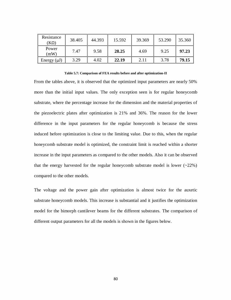
80
Resistance
(KΩ) 38.405 44.393 15.592 39.369 53.290 35.360
Power
(mW) 7.47 9.58 28.25 4.69 9.25 97.23
Energy (μJ) 3.29 4.02 22.19 2.11 3.78 79.15
Table 5.7: Comparison of FEA results before and after optimization-II
From the tables above, it is observed that the optimized input parameters are nearly 50%
more than the initial input values. The only exception seen is for regular honeycomb
substrate, where the percentage increase for the dimension and the material properties of
the piezoelectric plates after optimization is 21% and 36%. The reason for the lower
difference in the input parameters for the regular honeycomb is because the stress
induced before optimization is close to the limiting value. Due to this, when the regular
honeycomb substrate model is optimized, the constraint limit is reached within a shorter
increase in the input parameters as compared to the other models. Also it can be observed
that the energy harvested for the regular honeycomb substrate model is lower (~22%)
compared to the other models.
The voltage and the power gain after optimization is almost twice for the auxetic
substrate honeycomb models. This increase is substantial and it justifies the optimization
model for the bimorph cantilever beams for the different substrates. The comparison of
different output parameters for all the models is shown in the figures below.

81
Figure 5.17: Relation between electrical potential and frequency (Before and after optimization)
Source Voltage (V), Vs
Before
Optimization After
Optimization % Change
Solid homogenous substrate
3.12 4.45 42.63
Regular honeycomb substrate
23.96 29.17 21.74
Auxetic honeycomb substrate
19.2 28.3 47.40
Table 5.8: Comparison of optimization results for Source Voltage
0
5
10
15
20
25
30
35
100 120 140 160 180 200
Ep
ot
(V)
Frequency (Hz)
Solid-Before
Solid-After
Regular Honeycomb- Before
Regular Honeycomb-After
Auxetic Honeycomb-Before
Auxetic Honeycomb-After

82
Figure 5.18: Relation between voltage and frequency (Before and after optimization)
Load Voltage (V),VL
Before
Optimization After
Optimization % Change
Solid homogenous substrate
2.21 3.14 42.08
Regular honeycomb substrate
16.94 20.63 21.78
Auxetic honeycomb substrate
13.58 20 47.28
Table 5.9: Comparison of optimization results for Load Voltage
0
5
10
15
20
25
100 120 140 160 180 200
Lo
ad
Vo
ltag
e (V
)
Frequency (Hz)
Solid-Before Solid-After
Regular Honeycomb- Before Regular Honeycomb-After
Auxetic Honeycomb-Before Auxetic Honeycomb-After
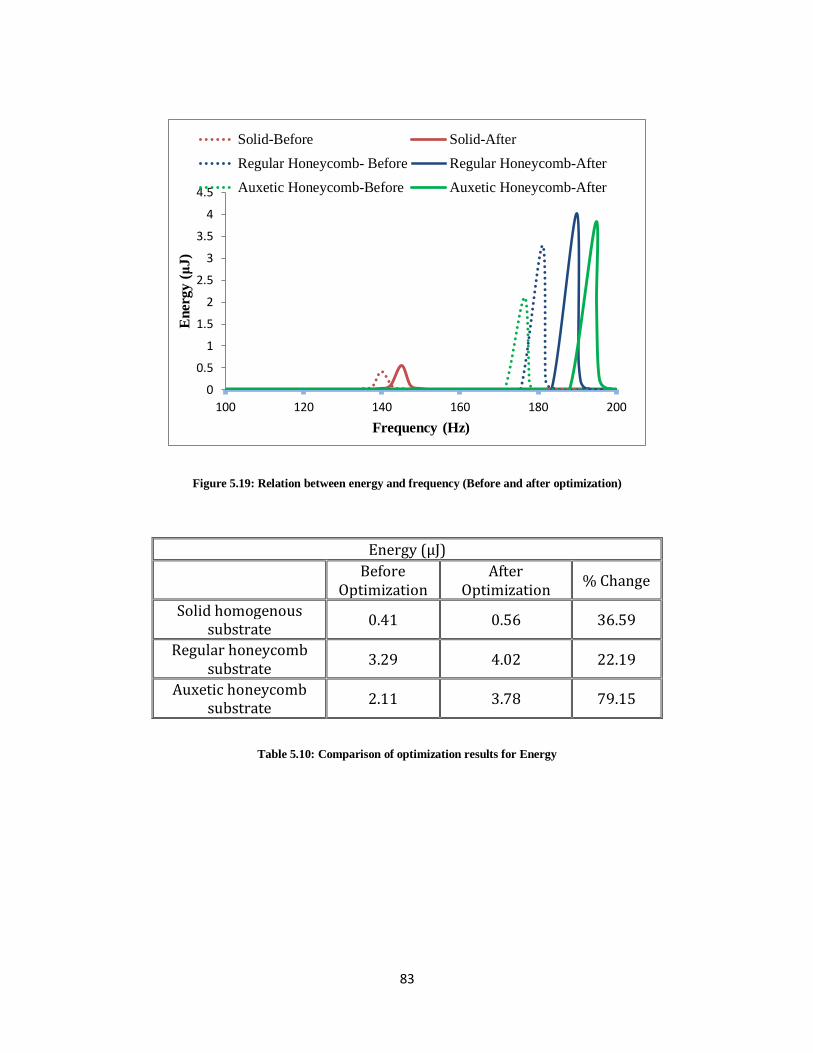
83
Figure 5.19: Relation between energy and frequency (Before and after optimization)
Energy (μJ)
Before
Optimization After
Optimization % Change
Solid homogenous substrate
0.41 0.56 36.59
Regular honeycomb substrate
3.29 4.02 22.19
Auxetic honeycomb substrate
2.11 3.78 79.15
Table 5.10: Comparison of optimization results for Energy
0
0.5
1
1.5
2
2.5
3
3.5
4
4.5
100 120 140 160 180 200
En
erg
y (μ
J)
Frequency (Hz)
Solid-Before Solid-After
Regular Honeycomb- Before Regular Honeycomb-After
Auxetic Honeycomb-Before Auxetic Honeycomb-After
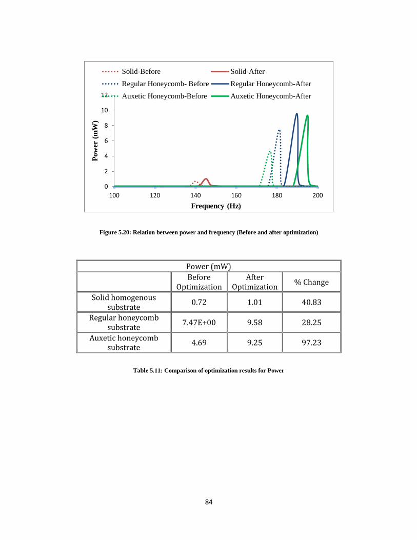
84
Figure 5.20: Relation between power and frequency (Before and after optimization)
Power (mW)
Before
Optimization After
Optimization % Change
Solid homogenous substrate
0.72 1.01 40.83
Regular honeycomb substrate
7.47E+00 9.58 28.25
Auxetic honeycomb substrate
4.69 9.25 97.23
Table 5.11: Comparison of optimization results for Power
0
2
4
6
8
10
12
100 120 140 160 180 200
Po
wer
(m
W)
Frequency (Hz)
Solid-Before Solid-After
Regular Honeycomb- Before Regular Honeycomb-After
Auxetic Honeycomb-Before Auxetic Honeycomb-After

85
Figure 5.21: Relation between stress and frequency (Before and after optimization)
Stress (Mpa)
Before
Optimization After
Optimization % Change
Solid homogenous substrate
7.763 9.843 26.789
Regular honeycomb substrate
69.153 6.88E+01 0.503
Auxetic honeycomb substrate
55.678 57.591 3.436
Table 5.12: Comparison of optimization results for stress
0
10
20
30
40
50
60
70
80
100 120 140 160 180 200
Str
ess,
S1
1 (
MP
a)
Frequency (Hz)
Solid-Before Solid-After
Regular Honeycomb- Before Regular Honeycomb-After
Auxetic Honeycomb-Before Auxetic Honeycomb-After

86
CHAPTER 6: CONCLUSION AND RECOMMENDATIONS FOR
FUTURE WORK
In this thesis, the design and finite element analysis of the bimorph cantilever beam is
studied. The substrate used in the bimorph cantilever beam for this study is brass and the
piezoelectric plate material used is Lead Zirconate Titanate (PZT-5H). Three different
geometries of brass substrates were analyzed and compared in this study- solid
homogenous, regular hexagonal honeycomb and an auxetic hexagonal honeycomb. Also
an optimization study is conducted by linking the finite element software, ABAQUS to
the commercial optimization software, VisualDOC.
It is found that using the honeycomb material as a substrate is more efficient for
energy harvesting compared to a solid homogenous beam. The energy harvested
using the honeycomb brass substrate is nearly 8 times more than using the solid
homogenous plate with the increase in the load voltage generated as high as 8
times for the same applied load and boundary conditions. The main factor
contributing to this is the lower mass of the honeycomb beams. It is observed that
the mass of the regular and the auxetic honeycomb is lower than that of the solid
beam substrate by a factor of 6.3 and 4.5 respectively. As the mass reduce, the
cantilever beam vibrates with higher amplitude. As the frequency of vibration
increases, the resistance reduces and power, which is inversely proportional to the
resistance, increases.
87
The optimization variables selected were the depth and the piezoelectric strain
constant in the x direction, d31. These parameters were found to be the critical
factors affecting the energy harvesting performance of bimorph cantilever beam
in a sensitive analysis study done in a previous research [12]. Hence these
parameters were optimized with the ultimate tensile strength of the piezoelectric
plate as the constraining limit. It is observed that by the input and output
parameters increase substantially after optimization for all three types of
substrates. This proves that optimization helps to increase the efficiency of
harvesting energy from a vibrating bimorph cantilever beam in terms of utilizing
the dimensional and material parameters within the constraint limits
The results of optimization were verified by analyzing all three types of substrates
with the input parameters obtained from the optimization results. The output
parameters of the analysis results vary from the results of optimization software.
The reason for this variation is that VisualDOC optimizes only two parameters of
the ABAQUS model. However, the output of the ABAQUS depends on all the
material and geometric parameters of both the substrate and the piezoelectric
beams.
VisualDOC is found to be an effective tool in optimizing the parameters for the
bimorph cantilever beam problem as the convergence is obtained after a few
iterations for the given population size. The best estimates of the required output
parameters are plotted to visualize the relationship between the parameters and
the number of iterations. The maximum stress value for the solid substrate models

88
is less than the constraint stress because of the limits given for the input
parameters. These limits are selected to maintain consistency across all the four
models analyzed such that the optimized stress does not exceed the constraint
limit for any of these models.
Recommendations for Future Work
The thesis can be extended to constructing a finite element model of the bimorph
beam by replacing the solid brass substrate with honeycomb geometry (regular
and auxetic) with in-plane and out–of-plane configuration, with wall thickness of
the substrate as an additional design variable and comparing the optimization
results with the solid brass substrate configuration.
This work is limited to the use of brass as the substrate material with three
different types of geometries. Research can be extending the use of different
materials as the substrate and also different types of honeycomb geometries such
as square honeycombs, triangular honeycombs, chiral honeycombs etc.
Research can also be extended by varying the electrical configuration of the
bimorph cantilever beam assembly. Research has already been done by
assembling the beam plates in parallel and series configuration for a solid beam
substrate. This work can be extended to the use of honeycomb substrates and a
comparison study with the in-plane and out-of-plane loading conditions can be
done to identify the optimal combination that can harvest the maximum energy.

89
REFERENCES
1. Choi, W.J., Jeon, Y., Jeong, J.-H., Sood, R., and Kim, S.G., 2006, “Energy harvesting
MEMS device based on thin film piezoelectric cantilevers”, Journal of Electro-
ceramics, 17:543-548.
2. Erturk, A. and Inman, D.J., 2008, “A Distributed Parameter Electromechanical Model
for Cantilevered Piezoelectric Energy Harvesters”, Transactions of the ASME:
Journal of Vibration and Acoustics, 130: 041002.
3. Wang, D., 2009, “Impact behavior and energy absorption of paper honeycomb
sandwich panels”, International Journal of Impact Engineering, 36:1, pp. 110–114.
4. Erturk, A. and Inman, D.J., 2009, “An experimentally validated bimorph cantilever
model for piezoelectric energy harvesting from base excitations”, Smart Materials
and Structures, 18, 025009.
5. Kim, S., Clark, W.W., and Wang, Q.M., 2005, “Piezoelectric Energy Harvesting with
a Clamped Circular Plate: Analysis”, Journal of Intelligent Material Systems and
Structures, 16:847-854.
6. Liao, Y. and Sodano, H.A., 2008, “Model of a single mode energy harvester and
properties for optimal power generation”, Smart Materials Structures, 17:065026.
7. Roundy, S. and Wright, P.K., 2004, “A Piezoelectric Vibration Based Generator for
Wireless Electronics”, Smart Materials and Structures, 13:1131-1142.
8. Mansour, M.O., Arafa, M.H., and Megahed, S.M., 2010, “Design of vibration based
energy harvesters with adjustable natural frequency”, International Design
engineering technical conferences & Computers and information in engineering
conference, ASME 2010-28429.
9. Shu, Y.C. and Lien, J., 2006, “Efficiency of energy conversion for a piezoelectric
power harvesting system”, Journal of Micromechanics and Micro engineering,
16:2429–2438.
10. Ertuk, A., Inman, D.J., 2011, “Piezoelectric Energy Harvesting”, John Wiley & Sons,
Sussex, U.K.
11. Sodano, H.A., Park, G. and Inman, D.J., 2004, “Estimation of Electric Charge Output
for Piezoelectric Energy Harvesting”, Strain, 40:49-58.

90
12. Chandrasekharan, N., Jaehyung, Ju., Thompson, L., 2013, “Effect of Geometrical and
Material Properties on Electrical Power Harvested from a Bimorph Piezoelectric
Cantilever beam”, Multidiscipline Modeling in Material and Structures.
13. Galgalikar, R.R., 2012, “Design Automation and Optimization of honeycomb
structures for maximum sound transmission loss”, Clemson University.
14. Seera, N. K., 2011, “Viscoelastic damping of hexagonal honeycomb sandwich
panels”, Clemson University.
15. Telukunta, R., 2011, “Constrained layer damping of honeycomb composite
structures”, Clemson University.
16. Evans, K. E., and Alderson, K. L., 2000, “Auxetic materials : the positive side of
being negative”, Engineering Science and Education Journal, (August), pp. 148–154.
17. Masters, I. G. and Evans, K. E., 1996, “Models for the Elastic Deformation of
Honeycombs”, Composite Structures, 35:403–422.
18. Sodano, H.A. and Inman, D.J., 2005, “Generation and Storage of Electricity from
Power Harvesting Devices”, Journal of Intelligent material systems and structures,
16:16-67.
19. Sodano, H.A, Inman, D.J., Park,G., 2005, “Comparison of Piezoelectric Energy
Harvesting Devices for Recharging Batteries”, Journal of Sound and Vibration, 16:
799-807.
20. Roundy, S., Leland, E.S., Baker, J., Carleton, E., Reilly, E., Lai, E., Otis, B., Rabaey,
J.M., and Wright, P.K., “Improving the power output for vibration based energy
scavengers”, IEEE CS and IEEE ComSoc 1536-1268, 2005.
21. Renno, J.M., Daqaq, M.F., and Inman, D.J., 2008, “On the Optimal Energy
Harvesting from a Vibration Source”, Journal of Sound and Vibration, 320:386-405.
22. Ahmed, K.M., 1971, “Static and Dynamic Analysis of Sandwich Structures by the
Method of Finite Elements”, Journal of sound and Vibration, 18:75-91.
23. Nabarrette, A., Almeida, S.D.M., and Hansen, J.S., 2003, “Sandwich-Plate Vibration
Analysis: Three-Layer Quasi-Three-Dimensional Finite Element Model”, AIAA
Journal, 41:1547-1555.
24. Amichi, K. and Atalla, N., 2009, “A New 3D Finite Element for Sandwich Beams
with a Viscoelastic Core”, The Transactions of the ASME: Journal of Vibration and
Acoustics, 131:1-9

91
25. Gibson, L. J. and Ashby, M.F., 1988, “Cellular Solids: Structures and Properties”,
Pergamon, Oxford, England, U.K.
26. Grediac, M, 1993, “A Finite Element Study of the Transverse Shear in Honeycomb
Cores,” International Journal of Solids and Structures, 30:1777-1788
27. Ruzzene, M. and Scarpa, F., 2003, “Control of Wave Propagation in Sandwich Beams
with Auxetic Core”, Journal of Intelligent Material Systems and Structures, 14: 443-
453.
28. Ikeda, T., 1996, “Fundamentals of Piezoelectricity”, Oxford University Press, New
York.
29. Gibson, L.J. and Ashby, M.F., 1997, “Cellular Solids: Structure and properties”,
Cambridge University Press, Cambridge, U.K.
30. Yamashita, M., and Gotoh, M., 2005, “Impact behavior of honeycomb structures with
various cell specifications numerical simulation and experiment”, International
Journal of Impact Engineering, 32(1-4):618–630.
31. Fisher, R.A, 1951, “Design of Experiments”, 6th edition, Oliver & Boyd, London,
U.K.
32. Overvelde, J. T. B., 2010, “Learn Abaqus script in one hour”, pp. 1–12.
33. Piezoceramics- Technical description and Material characteristics, 2011, Nolaic A/S,
Retrieved, May 20, 2013, from http://www.noliac.com/Technical_description-
6585.aspx.
34. Choi, S.B., Han, Y.M., 2010, “Piezoelectric Actuators-Control Applications of Smart
Materials”, CRC Press, Florida, USA.
35. Ertuk, A., Inman, D.J., 2011, “Piezoelectric Energy Harvesting”, John Wiley and
Sons, Ltd, Publication, West Sussex, U.K.
36. Ju, J., Summers, J. D., Ziegert, J., and Fadel, G., 2012, “Design of Honeycombs for
Modulus and Yield Strain in Shear”, Journal of Engineering Materials and
Technology, 134(1), p. 011002.
37. Chee, C. Y. K, Tong, L., and Steven, G. P., 1999, “A mixed model for composite
beams with piezoelectric actuators and sensors”, Smart Mater. Struct. 8 417–32

92
38. Beheshti-Aval, S. B., Lezgy-Nazargah, M., Vidal, P., and Polit, O., 2011, “ A refined
sinus finite element model for the analysis of piezoelectric-laminated beams”, J.
Intell. Mater. Syst. Struct. 22 203
39. Elshafei, M. A., Bendary, I. M., and Riad, A. M., 2010, “Finite element model of
smart beams with distributed piezoelectric actuators”, J. Intell. Mater. Syst. Struct. 21
747–58
40. Saravanos, D. A., and Heyliger, P. R., 1995, “Coupled layer wise analysis of
composite beams with embedded piezoelectric sensors and actuators”, J. Intell. Mater.
Syst. Struct. 6 350–63
41. Robbins, D. H., and Reddy, J. N., 1991, “Analysis of piezo-electrically actuated
beams using a layer-wise displacement theory”, J. Comput. Struct. 41 265–79
42. Elshafei, M.A., and Alraiess, F., 2013, “Modeling and Analysis of smart piezoelectric
beams using simple higher order shear deformation theory”, Smart Mater. Struct. 22
035006.
43. Dassault Systems and Simulia, ABAQUS Example Problems Manual.
44. “http://abaqus.civil.uwa.edu.au:2080/v6.9/”.
45. VisualDOC User Manual, Version 7.1, Nov. 2012, Vanderplaats Research and
Development, Inc., Colorado,USA.
46. Elements of Structural Optimization – Haftka and Gurdal, Kluwer, 1996
47. Genetic Algorithms in Search, Optimization and Machine learning. Goldberg,
Addison Wesley, 1992.
48. Optimization concepts and applications in engineering by Belegundu, Chandrupatla
Prentice Hall, 1999

93
APPENDICES
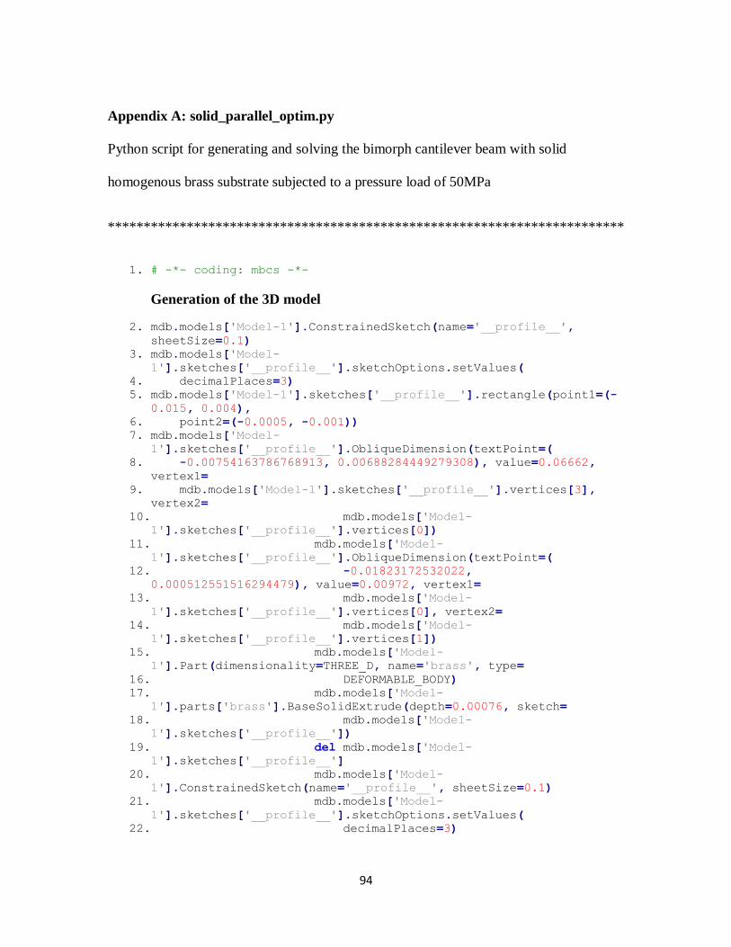
94
Appendix A: solid_parallel_optim.py
Python script for generating and solving the bimorph cantilever beam with solid
homogenous brass substrate subjected to a pressure load of 50MPa
************************************************************************
1. # -*- coding: mbcs -*-
Generation of the 3D model
2. mdb.models['Model-1'].ConstrainedSketch(name='__profile__', sheetSize=0.1)
3. mdb.models['Model-1'].sketches['__profile__'].sketchOptions.setValues(
4. decimalPlaces=3) 5. mdb.models['Model-1'].sketches['__profile__'].rectangle(point1=(-
0.015, 0.004),
6. point2=(-0.0005, -0.001)) 7. mdb.models['Model-
1'].sketches['__profile__'].ObliqueDimension(textPoint=(
8. -0.00754163786768913, 0.00688284449279308), value=0.06662, vertex1=
9. mdb.models['Model-1'].sketches['__profile__'].vertices[3], vertex2=
10. mdb.models['Model-
1'].sketches['__profile__'].vertices[0])
11. mdb.models['Model-
1'].sketches['__profile__'].ObliqueDimension(textPoint=(
12. -0.01823172532022,
0.000512551516294479), value=0.00972, vertex1=
13. mdb.models['Model-
1'].sketches['__profile__'].vertices[0], vertex2=
14. mdb.models['Model-
1'].sketches['__profile__'].vertices[1])
15. mdb.models['Model-
1'].Part(dimensionality=THREE_D, name='brass', type=
16. DEFORMABLE_BODY)
17. mdb.models['Model-
1'].parts['brass'].BaseSolidExtrude(depth=0.00076, sketch=
18. mdb.models['Model-
1'].sketches['__profile__'])
19. del mdb.models['Model-
1'].sketches['__profile__']
20. mdb.models['Model-
1'].ConstrainedSketch(name='__profile__', sheetSize=0.1)
21. mdb.models['Model-
1'].sketches['__profile__'].sketchOptions.setValues(
22. decimalPlaces=3)
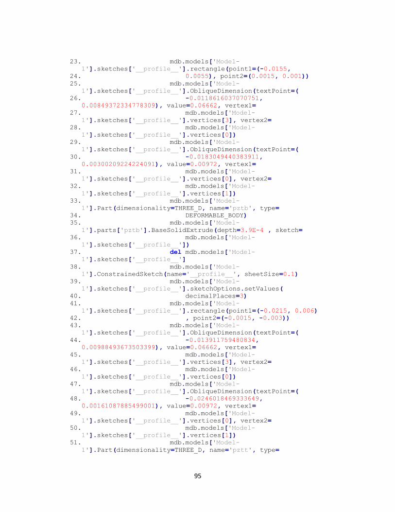
95
23. mdb.models['Model-
1'].sketches['__profile__'].rectangle(point1=(-0.0155,
24. 0.0055), point2=(0.0015, 0.001))
25. mdb.models['Model-
1'].sketches['__profile__'].ObliqueDimension(textPoint=(
26. -0.0118616037070751,
0.00849372334778309), value=0.06662, vertex1=
27. mdb.models['Model-
1'].sketches['__profile__'].vertices[3], vertex2=
28. mdb.models['Model-
1'].sketches['__profile__'].vertices[0])
29. mdb.models['Model-
1'].sketches['__profile__'].ObliqueDimension(textPoint=(
30. -0.0183049440383911,
0.00300209224224091), value=0.00972, vertex1=
31. mdb.models['Model-
1'].sketches['__profile__'].vertices[0], vertex2=
32. mdb.models['Model-
1'].sketches['__profile__'].vertices[1])
33. mdb.models['Model-
1'].Part(dimensionality=THREE_D, name='pztb', type=
34. DEFORMABLE_BODY)
35. mdb.models['Model-
1'].parts['pztb'].BaseSolidExtrude(depth=3.9E-4 , sketch=
36. mdb.models['Model-
1'].sketches['__profile__'])
37. del mdb.models['Model-
1'].sketches['__profile__']
38. mdb.models['Model-
1'].ConstrainedSketch(name='__profile__', sheetSize=0.1)
39. mdb.models['Model-
1'].sketches['__profile__'].sketchOptions.setValues(
40. decimalPlaces=3)
41. mdb.models['Model-
1'].sketches['__profile__'].rectangle(point1=(-0.0215, 0.006)
42. , point2=(-0.0015, -0.003))
43. mdb.models['Model-
1'].sketches['__profile__'].ObliqueDimension(textPoint=(
44. -0.013911759480834,
0.00988493673503399), value=0.06662, vertex1=
45. mdb.models['Model-
1'].sketches['__profile__'].vertices[3], vertex2=
46. mdb.models['Model-
1'].sketches['__profile__'].vertices[0])
47. mdb.models['Model-
1'].sketches['__profile__'].ObliqueDimension(textPoint=(
48. -0.0246018469333649,
0.00161087885499001), value=0.00972, vertex1=
49. mdb.models['Model-
1'].sketches['__profile__'].vertices[0], vertex2=
50. mdb.models['Model-
1'].sketches['__profile__'].vertices[1])
51. mdb.models['Model-
1'].Part(dimensionality=THREE_D, name='pztt', type=

96
52. DEFORMABLE_BODY)
53. mdb.models['Model-
1'].parts['pztt'].BaseSolidExtrude(depth=0.00026, sketch=
54. mdb.models['Model-
1'].sketches['__profile__'])
55. del mdb.models['Model-
1'].sketches['__profile__']
56. mdb.models['Model-
1'].Material(name='brass')
Assigning Material properties
57. mdb.models['Model-
1'].materials['brass'].Density(table=((8740.0, ), ))
58. mdb.models['Model-
1'].materials['brass'].Elastic(table=((97000000000.0, 0.34),
59. ))
60. mdb.models['Model-
1'].materials['brass'].Damping(alpha=17.1, beta=2.111e-05)
61. mdb.models['Model-1'].Material(name='pzt')
62. mdb.models['Model-
1'].materials['pzt'].Density(table=((7800.0, ), ))
63. mdb.models['Model-
1'].materials['pzt'].Elastic(table=((62000000000.0,
64. 62000000000.0, 49000000000.0, 0.289,
0.512, 0.512, 23500000000.0,
65. 23000000000.0, 23000000000.0), ),
type=ENGINEERING_CONSTANTS)
66. mdb.models['Model-
1'].materials['pzt'].Dielectric(table=((3.89e-08, 3.89e-08,
67. 3.36e-08), ), type=ORTHOTROPIC)
68. mdb.models['Model-
1'].materials['pzt'].Piezoelectric(table=((0.0, 0.0, 0.0,
69. 0.0, 0.0, 0.0, 0.0, 0.0, 0.0, 0.0, 0.0,
0.0, -4.8E-10, -3.2e-10, 6.5e-10,
70. 0.0, 0.0, 0.0), ), type=STRAIN)
Defining Sections properties for brass and pzt
71. mdb.models['Model-
1'].HomogeneousSolidSection(material='brass', name='brass',
72. thickness=None)
73. mdb.models['Model-
1'].HomogeneousSolidSection(material='pzt', name='pzt',
74. thickness=None)
Assigning section properties and material orientation
75. mdb.models['Model-
1'].parts['brass'].Surface(name='bt', side1Faces=
76. mdb.models['Model-
1'].parts['brass'].faces.getSequenceFromMask(('[#10 ]',
77. ), ))
97
78. mdb.models['Model-
1'].parts['brass'].Surface(name='bb', side1Faces=
79. mdb.models['Model-
1'].parts['brass'].faces.getSequenceFromMask(('[#20 ]',
80. ), ))
81. mdb.models['Model-
1'].parts['brass'].SectionAssignment(offset=0.0, offsetField=
82. '', offsetType=MIDDLE_SURFACE,
region=Region(
83. cells=mdb.models['Model-
1'].parts['brass'].cells.getSequenceFromMask(mask=(
84. '[#1 ]', ), )), sectionName='brass',
thicknessAssignment=FROM_SECTION)
85. mdb.models['Model-
1'].parts['brass'].MaterialOrientation(
86. additionalRotationType=ROTATION_NONE,
axis=AXIS_1, fieldName='', localCsys=
87. None, orientationType=GLOBAL,
region=Region(
88. cells=mdb.models['Model-
1'].parts['brass'].cells.getSequenceFromMask(mask=(
89. '[#1 ]', ), )), stackDirection=STACK_3)
Meshing the brass substrate
90. mdb.models['Model-
1'].parts['brass'].seedPart(deviationFactor=0.1, size=0.0034)
91. mdb.models['Model-
1'].parts['brass'].setElementType(elemTypes=(ElemType(
92. elemCode=C3D20R, elemLibrary=STANDARD),
ElemType(elemCode=C3D15,
93. elemLibrary=STANDARD),
ElemType(elemCode=C3D10, elemLibrary=STANDARD)),
94. regions=(mdb.models['Model-
1'].parts['brass'].cells.getSequenceFromMask((
95. '[#1 ]', ), ), ))
96. mdb.models['Model-
1'].parts['brass'].generateMesh()
Meshing the pzt plates
97. mdb.models['Model-
1'].parts['pztb'].Surface(name='pbt', side1Faces=
98. mdb.models['Model-
1'].parts['pztb'].faces.getSequenceFromMask(('[#10 ]', ),
99. ))
100. mdb.models['Model-
1'].parts['pztb'].Surface(name='pbb', side1Faces=
101. mdb.models['Model-
1'].parts['pztb'].faces.getSequenceFromMask(('[#20 ]', ),
102. ))

98
103. mdb.models['Model-
1'].parts['pztb'].SectionAssignment(offset=0.0, offsetField=
104. '', offsetType=MIDDLE_SURFACE,
region=Region(
105. cells=mdb.models['Model-
1'].parts['pztb'].cells.getSequenceFromMask(mask=(
106. '[#1 ]', ), )), sectionName='pzt',
thicknessAssignment=FROM_SECTION)
107. mdb.models['Model-
1'].parts['pztb'].MaterialOrientation(additionalRotationType=
108. ROTATION_NONE, axis=AXIS_1,
fieldName='', localCsys=None, orientationType=
109. GLOBAL, region=Region(
110. cells=mdb.models['Model-
1'].parts['pztb'].cells.getSequenceFromMask(mask=(
111. '[#1 ]', ), )), stackDirection=STACK_3)
112. mdb.models['Model-
1'].parts['pztb'].seedPart(deviationFactor=0.1, size=0.0034)
113. mdb.models['Model-
1'].parts['pztb'].setElementType(elemTypes=(ElemType(
114. elemCode=C3D20RE,
elemLibrary=STANDARD), ElemType(elemCode=C3D15E,
115. elemLibrary=STANDARD),
ElemType(elemCode=C3D10E, elemLibrary=STANDARD)),
116. regions=(mdb.models['Model-
1'].parts['pztb'].cells.getSequenceFromMask((
117. '[#1 ]', ), ), ))
118. mdb.models['Model-
1'].parts['pztb'].generateMesh()
119. mdb.models['Model-
1'].parts['pztt'].Surface(name='ptt', side1Faces=
120. mdb.models['Model-
1'].parts['pztt'].faces.getSequenceFromMask(('[#10 ]', ),
121. ))
122. mdb.models['Model-
1'].parts['pztt'].Surface(name='ptb', side1Faces=
123. mdb.models['Model-
1'].parts['pztt'].faces.getSequenceFromMask(('[#20 ]', ),
124. ))
125. mdb.models['Model-
1'].parts['pztt'].SectionAssignment(offset=0.0, offsetField=
126. '', offsetType=MIDDLE_SURFACE,
region=Region(
127. cells=mdb.models['Model-
1'].parts['pztt'].cells.getSequenceFromMask(mask=(
128. '[#1 ]', ), )), sectionName='pzt',
thicknessAssignment=FROM_SECTION)
129. mdb.models['Model-
1'].parts['pztt'].MaterialOrientation(additionalRotationType=
130. ROTATION_NONE, axis=AXIS_1,
fieldName='', localCsys=None, orientationType=
131. GLOBAL, region=Region(
132. cells=mdb.models['Model-
1'].parts['pztt'].cells.getSequenceFromMask(mask=(
99
133. '[#1 ]', ), )), stackDirection=STACK_3)
134. mdb.models['Model-
1'].parts['pztt'].seedPart(deviationFactor=0.1, size=0.0034)
135. mdb.models['Model-
1'].parts['pztt'].setElementType(elemTypes=(ElemType(
136. elemCode=C3D20RE,
elemLibrary=STANDARD), ElemType(elemCode=C3D15E,
137. elemLibrary=STANDARD),
ElemType(elemCode=C3D10E, elemLibrary=STANDARD)),
138. regions=(mdb.models['Model-
1'].parts['pztt'].cells.getSequenceFromMask((
139. '[#1 ]', ), ), ))
140. mdb.models['Model-
1'].parts['pztt'].generateMesh()
Generating master and slave node sets for equation constraint
141. mdb.models['Model-
1'].rootAssembly.DatumCsysByDefault(CARTESIAN)
142. mdb.models['Model-
1'].rootAssembly.Instance(dependent=ON, name='pztb-1', part=
143. mdb.models['Model-1'].parts['pztb'])
144. mdb.models['Model-
1'].rootAssembly.Instance(dependent=ON, name='brass-1', part=
145. mdb.models['Model-1'].parts['brass'])
146. mdb.models['Model-
1'].rootAssembly.instances['brass-1'].translate(vector=(
147. 0.07278200182271, 0.0, 0.0))
148. mdb.models['Model-
1'].rootAssembly.translate(instanceList=('brass-1', ),
149. vector=(-0.073282, 0.0015, 0.00026))
150. mdb.models['Model-
1'].rootAssembly.Instance(dependent=ON, name='pztt-1', part=
151. mdb.models['Model-1'].parts['pztt'])
152. mdb.models['Model-
1'].rootAssembly.instances['pztt-1'].translate(vector=(
153. 0.079282002709806, 0.0, 0.0))
154. mdb.models['Model-
1'].rootAssembly.translate(instanceList=('pztt-1', ), vector=
155. (-0.073282, -0.0005, 0.00102))
Assembling the bimorph cantiveler beam
156. mdb.models['Model-
1'].rootAssembly.Set(name='tm', nodes=
157. mdb.models['Model-
1'].rootAssembly.instances['pztt-1'].nodes.getSequenceFromMask(
158. mask=('[#0:5 #800000 ]', ), ))
159. mdb.models['Model-
1'].rootAssembly.Set(name='ts', nodes=
160. mdb.models['Model-
1'].rootAssembly.instances['pztt-1'].nodes.getSequenceFromMask(
161. mask=(

100
162. '[#f0f0f0f:5 #c443180f #e18c384
#e18c3863 #18c38630 #8c38630e #c38630e1',
163. ' #38630e18 #8630e18c #630e18c3
#30e18c38 #e18c386 #18c3863 ]', ), ))
164. mdb.models['Model-
1'].rootAssembly.Set(name='bm', nodes=
165. mdb.models['Model-
1'].rootAssembly.instances['pztb-1'].nodes.getSequenceFromMask(
166. mask=('[#0:5 #2000000 ]', ), ))
167. mdb.models['Model-
1'].rootAssembly.Set(name='bs', nodes=
168. mdb.models['Model-
1'].rootAssembly.instances['pztb-1'].nodes.getSequenceFromMask(
169. mask=(
170. '[#f0f0f0f0:5 #181c42f0 #70a31c2a
#a31c28c #a31c28c7 #31c28c70 #1c28c70a',
171. ' #c28c70a3 #28c70a31 #8c70a31c
#c70a31c2 #70a31c28 #231c28c ]', ), ))
Defining Steps
172. mdb.models['Model-
1'].FrequencyStep(acousticCoupling=AC_OFF, eigensolver=
173. SUBSPACE, maxIterations=30, name='f',
normalization=DISPLACEMENT, numEigen=
174. 10, previous='Initial',
simLinearDynamics=OFF, vectors=18)
175. mdb.models['Model-
1'].steps['f'].setValues(maxEigen=1000.0, normalization=MASS)
176. mdb.models['Model-
1'].SteadyStateDirectStep(frequencyRange=((100.0, 200.0, 20,
177. 1.0), ), frictionDamping=ON,
matrixStorage=SYMMETRIC, name='dy', previous=
178. 'f', subdivideUsingEigenfrequencies=ON)
Requesting field output
179. mdb.models['Model-
1'].fieldOutputRequests['F-Output-1'].setValues(rebar=EXCLUDE
180. , region=mdb.models['Model-
1'].rootAssembly.sets['bm'], sectionPoints=
181. DEFAULT, variables=('S', 'EPOT'))
182. mdb.models['Model-
1'].fieldOutputRequests['F-Output-2'].setValues(variables=(
183. 'S', 'EPOT'))
Defining Constraints
184. mdb.models['Model-1'].Tie(adjust=ON,
master=
185. mdb.models['Model-
1'].rootAssembly.instances['brass-1'].surfaces['bt'],

101
186. name='Constraint-1',
positionToleranceMethod=COMPUTED, slave=
187. mdb.models['Model-
1'].rootAssembly.instances['pztt-1'].surfaces['ptb'],
188. thickness=ON, tieRotations=ON)
189. mdb.models['Model-1'].Tie(adjust=ON,
master=
190. mdb.models['Model-
1'].rootAssembly.instances['brass-1'].surfaces['bb'],
191. name='Constraint-2',
positionToleranceMethod=COMPUTED, slave=
192. mdb.models['Model-
1'].rootAssembly.instances['pztb-1'].surfaces['pbt'],
193. thickness=ON, tieRotations=ON)
194. mdb.models['Model-
1'].rootAssembly.features['brass-1'].suppress()
195. mdb.models['Model-
1'].Equation(name='Constraint-3', terms=((-1.0, 'bs', 9), (
196. 1.0, 'bm', 9)))
197. mdb.models['Model-
1'].Equation(name='Constraint-4', terms=((-1.0, 'ts', 9), (
198. 1.0, 'tm', 9)))
Assigning loading conditions
199. mdb.models['Model-
1'].Pressure(amplitude=UNSET, createStepName='dy',
200. distributionType=UNIFORM, field='',
magnitude=(16+0j), name='Load-1',
201. region=Region(
202. side1Faces=mdb.models['Model-
1'].rootAssembly.instances['pztb-1'].faces.getSequenceFromMask(
203. mask=('[#20 ]', ), )))
204. mdb.models['Model-
1'].ElectricPotentialBC(createStepName='Initial',
205. distributionType=UNIFORM, fieldName='',
magnitude=0.0, name='BC-1', region=
206. Region(
207. faces=mdb.models['Model-
1'].rootAssembly.instances['pztt-1'].faces.getSequenceFromMask(
208. mask=('[#20 ]', ), )))
Assigning boundary conditions
209. mdb.models['Model-
1'].ElectricPotentialBC(createStepName='Initial',
210. distributionType=UNIFORM, fieldName='',
magnitude=0.0, name='BC-2', region=
211. Region(
212. faces=mdb.models['Model-
1'].rootAssembly.instances['pztb-1'].faces.getSequenceFromMask(
213. mask=('[#10 ]', ), )))

102
214. mdb.models['Model-
1'].rootAssembly.features['brass-1'].resume()
215. mdb.models['Model-
1'].EncastreBC(createStepName='Initial', localCsys=None,
216. name='BC-3', region=Region(
217. faces=mdb.models['Model-
1'].rootAssembly.instances['brass-1'].faces.getSequenceFromMask(
218. mask=('[#4 ]', ), )+\
219. mdb.models['Model-
1'].rootAssembly.instances['pztb-1'].faces.getSequenceFromMask(
220. mask=('[#4 ]', ), )+\
221. mdb.models['Model-
1'].rootAssembly.instances['pztt-1'].faces.getSequenceFromMask(
222. mask=('[#4 ]', ), ),
223. edges=mdb.models['Model-
1'].rootAssembly.instances['pztb-1'].edges.getSequenceFromMask(
224. mask=('[#200 ]', ), )))
225. mdb.Job(atTime=None, contactPrint=OFF,
description='', echoPrint=OFF,
226. explicitPrecision=SINGLE,
getMemoryFromAnalysis=True, historyPrint=OFF,
227. memory=90, memoryUnits=PERCENTAGE,
model='Model-1', modelPrint=OFF,
228. multiprocessingMode=DEFAULT,
name='solid16-job', nodalOutputPrecision=
229. SINGLE, numCpus=1, queue=None,
scratch='', type=ANALYSIS, userSubroutine=''
230. , waitHours=0, waitMinutes=0)
Executing the analysis
231. mdb.jobs['solid16-
job'].submit(consistencyChecking=OFF)
232. mdb.jobs['solid16-job']._Message(STARTED,
{'phase': BATCHPRE_PHASE,
233. 'clientHost': 'Jadesha-PC', 'handle':
0, 'jobName': 'solid16-job'})
234. mdb.jobs['solid16-job']._Message(WARNING,
{'phase': BATCHPRE_PHASE,
235. 'message': 'FOR *TIE PAIR
(ASSEMBLY_PZTT-1_PTB-ASSEMBLY_BRASS-1_BT), ADJUSTED NODES WITH
VERY SMALL ADJUSTMENTS WERE NOT PRINTED. SPECIFY
*PREPRINT,MODEL=YES FOR COMPLETE PRINTOUT.',
236. 'jobName': 'solid16-job'})
237. mdb.jobs['solid16-job']._Message(WARNING,
{'phase': BATCHPRE_PHASE,
238. 'message': 'FOR *TIE PAIR
(ASSEMBLY_PZTB-1_PBT-ASSEMBLY_BRASS-1_BB), ADJUSTED NODES WITH
VERY SMALL ADJUSTMENTS WERE NOT PRINTED. SPECIFY
*PREPRINT,MODEL=YES FOR COMPLETE PRINTOUT.',
239. 'jobName': 'solid16-job'})
240. mdb.jobs['solid16-job']._Message(WARNING,
{'phase': BATCHPRE_PHASE,

103
241. 'message': '26 nodes have dof on which
incorrect boundary conditions may have been specified. The nodes
have been identified in node set WarnNodeBCIncorrectDof.',
242. 'jobName': 'solid16-job'})
243. mdb.jobs['solid16-job']._Message(WARNING,
{'phase': BATCHPRE_PHASE,
244. 'message': '26 nodes have dof on which
incorrect boundary conditions may have been specified. The nodes
have been identified in node set WarnNodeBCIncorrectDof.',
245. 'jobName': 'solid16-job'})
246. mdb.jobs['solid16-job']._Message(ODB_FILE,
{'phase': BATCHPRE_PHASE,
247. 'file': 'C:\\Temp\\solid16-job.odb',
'jobName': 'solid16-job'})
248. mdb.jobs['solid16-job']._Message(COMPLETED,
{'phase': BATCHPRE_PHASE,
249. 'message': 'Analysis phase complete',
'jobName': 'solid16-job'})
250. mdb.jobs['solid16-job']._Message(STARTED,
{'phase': STANDARD_PHASE,
251. 'clientHost': 'Jadesha-PC', 'handle':
2368, 'jobName': 'solid16-job'})
252. mdb.jobs['solid16-job']._Message(STEP,
{'phase': STANDARD_PHASE, 'stepId': 1,
253. 'jobName': 'solid16-job'})
254. mdb.jobs['solid16-job']._Message(ODB_FRAME,
{'phase': STANDARD_PHASE,
255. 'step': 0, 'frame': 0, 'jobName':
'solid16-job'})
256. mdb.jobs['solid16-job']._Message(STATUS,
{'totalTime': 0.0, 'attempts': 1,
257. 'timeIncrement': 1e-36, 'increment': 0,
'stepTime': 0.0, 'step': 1,
258. 'jobName': 'solid16-job', 'severe': 0,
'iterations': 0,
259. 'phase': STANDARD_PHASE, 'equilibrium':
0})
260. mdb.jobs['solid16-
job']._Message(MEMORY_ESTIMATE, {'phase': STANDARD_PHASE,
261. 'jobName': 'solid16-job', 'memory':
57.6551237106323})
262. mdb.jobs['solid16-job']._Message(ODB_FRAME,
{'phase': STANDARD_PHASE,
263. 'step': 0, 'frame': 1, 'jobName':
'solid16-job'})
264. mdb.jobs['solid16-job']._Message(ODB_FRAME,
{'phase': STANDARD_PHASE,
265. 'step': 0, 'frame': 2, 'jobName':
'solid16-job'})
266. mdb.jobs['solid16-job']._Message(ODB_FRAME,
{'phase': STANDARD_PHASE,
267. 'step': 0, 'frame': 3, 'jobName':
'solid16-job'})

104
268. mdb.jobs['solid16-job']._Message(ODB_FRAME,
{'phase': STANDARD_PHASE,
269. 'step': 0, 'frame': 4, 'jobName':
'solid16-job'})
270. mdb.jobs['solid16-job']._Message(ODB_FRAME,
{'phase': STANDARD_PHASE,
271. 'step': 0, 'frame': 5, 'jobName':
'solid16-job'})
272. mdb.jobs['solid16-job']._Message(STATUS,
{'totalTime': 0.0, 'attempts': 1,
273. 'timeIncrement': 1e-36, 'increment': 1,
'stepTime': 1e-36, 'step': 1,
274. 'jobName': 'solid16-job', 'severe': 0,
'iterations': 0,
275. 'phase': STANDARD_PHASE, 'equilibrium':
0})
276. mdb.jobs['solid16-job']._Message(END_STEP,
{'phase': STANDARD_PHASE,
277. 'stepId': 1, 'jobName': 'solid16-job'})
278. mdb.jobs['solid16-job']._Message(STEP,
{'phase': STANDARD_PHASE, 'stepId': 2,
279. 'jobName': 'solid16-job'})
280. mdb.jobs['solid16-job']._Message(ODB_FRAME,
{'phase': STANDARD_PHASE,
281. 'step': 1, 'frame': 0, 'jobName':
'solid16-job'})
282. mdb.jobs['solid16-job']._Message(STATUS,
{'totalTime': 0.0, 'attempts': 0,
283. 'timeIncrement': 100.0, 'increment': 0,
'stepTime': 0.0, 'step': 2,
284. 'jobName': 'solid16-job', 'severe': 0,
'iterations': 0,
285. 'phase': STANDARD_PHASE, 'equilibrium':
0})
286. mdb.jobs['solid16-
job']._Message(MEMORY_ESTIMATE, {'phase': STANDARD_PHASE,
287. 'jobName': 'solid16-job', 'memory':
143.1667137146})
288. mdb.jobs['solid16-job']._Message(ODB_FRAME,
{'phase': STANDARD_PHASE,
289. 'step': 1, 'frame': 1, 'jobName':
'solid16-job'})
290. mdb.jobs['solid16-job']._Message(STATUS,
{'phase': STANDARD_PHASE, 'step': 2,
291. 'frequency': 100.0, 'increment': 1,
'jobName': 'solid16-job'})
292. mdb.jobs['solid16-job']._Message(ODB_FRAME,
{'phase': STANDARD_PHASE,
293. 'step': 1, 'frame': 2, 'jobName':
'solid16-job'})
294. mdb.jobs['solid16-job']._Message(STATUS,
{'phase': STANDARD_PHASE, 'step': 2,
295. 'frequency': 101.78568311609,
'increment': 2, 'jobName': 'solid16-job'})

105
296. mdb.jobs['solid16-job']._Message(ODB_FRAME,
{'phase': STANDARD_PHASE,
297. 'step': 1, 'frame': 3, 'jobName':
'solid16-job'})
298. mdb.jobs['solid16-job']._Message(STATUS,
{'phase': STANDARD_PHASE, 'step': 2,
299. 'frequency': 103.603252874092,
'increment': 3, 'jobName': 'solid16-job'})
300. mdb.jobs['solid16-job']._Message(ODB_FRAME,
{'phase': STANDARD_PHASE,
301. 'step': 1, 'frame': 4, 'jobName':
'solid16-job'})
302. mdb.jobs['solid16-job']._Message(STATUS,
{'phase': STANDARD_PHASE, 'step': 2,
303. 'frequency': 105.453278668385,
'increment': 4, 'jobName': 'solid16-job'})
304. mdb.jobs['solid16-job']._Message(ODB_FRAME,
{'phase': STANDARD_PHASE,
305. 'step': 1, 'frame': 5, 'jobName':
'solid16-job'})
306. mdb.jobs['solid16-job']._Message(STATUS,
{'phase': STANDARD_PHASE, 'step': 2,
307. 'frequency': 107.33634006093,
'increment': 5, 'jobName': 'solid16-job'})
308. mdb.jobs['solid16-job']._Message(ODB_FRAME,
{'phase': STANDARD_PHASE,
309. 'step': 1, 'frame': 6, 'jobName':
'solid16-job'})
310. mdb.jobs['solid16-job']._Message(STATUS,
{'phase': STANDARD_PHASE, 'step': 2,
311. 'frequency': 109.253026962828,
'increment': 6, 'jobName': 'solid16-job'})
312. mdb.jobs['solid16-job']._Message(ODB_FRAME,
{'phase': STANDARD_PHASE,
313. 'step': 1, 'frame': 7, 'jobName':
'solid16-job'})
314. mdb.jobs['solid16-job']._Message(STATUS,
{'phase': STANDARD_PHASE, 'step': 2,
315. 'frequency': 111.20393981912,
'increment': 7, 'jobName': 'solid16-job'})
316. mdb.jobs['solid16-job']._Message(ODB_FRAME,
{'phase': STANDARD_PHASE,
317. 'step': 1, 'frame': 8, 'jobName':
'solid16-job'})
318. mdb.jobs['solid16-job']._Message(STATUS,
{'phase': STANDARD_PHASE, 'step': 2,
319. 'frequency': 113.189689796898,
'increment': 8, 'jobName': 'solid16-job'})
320. mdb.jobs['solid16-job']._Message(ODB_FRAME,
{'phase': STANDARD_PHASE,
321. 'step': 1, 'frame': 9, 'jobName':
'solid16-job'})
322. mdb.jobs['solid16-job']._Message(STATUS,
{'phase': STANDARD_PHASE, 'step': 2,
106
323. 'frequency': 115.210898976756,
'increment': 9, 'jobName': 'solid16-job'})
324. mdb.jobs['solid16-job']._Message(ODB_FRAME,
{'phase': STANDARD_PHASE,
325. 'step': 1, 'frame': 10, 'jobName':
'solid16-job'})
326. mdb.jobs['solid16-job']._Message(STATUS,
{'phase': STANDARD_PHASE, 'step': 2,
327. 'frequency': 117.26820054768,
'increment': 10, 'jobName': 'solid16-job'})
328. mdb.jobs['solid16-job']._Message(ODB_FRAME,
{'phase': STANDARD_PHASE,
329. 'step': 1, 'frame': 11, 'jobName':
'solid16-job'})
330. mdb.jobs['solid16-job']._Message(STATUS,
{'phase': STANDARD_PHASE, 'step': 2,
331. 'frequency': 119.362239005403,
'increment': 11, 'jobName': 'solid16-job'})
332. mdb.jobs['solid16-job']._Message(ODB_FRAME,
{'phase': STANDARD_PHASE,
333. 'step': 1, 'frame': 12, 'jobName':
'solid16-job'})
334. mdb.jobs['solid16-job']._Message(STATUS,
{'phase': STANDARD_PHASE, 'step': 2,
335. 'frequency': 121.49367035431,
'increment': 12, 'jobName': 'solid16-job'})
336. mdb.jobs['solid16-job']._Message(ODB_FRAME,
{'phase': STANDARD_PHASE,
337. 'step': 1, 'frame': 13, 'jobName':
'solid16-job'})
338. mdb.jobs['solid16-job']._Message(STATUS,
{'phase': STANDARD_PHASE, 'step': 2,
339. 'frequency': 123.663162312946,
'increment': 13, 'jobName': 'solid16-job'})
340. mdb.jobs['solid16-job']._Message(ODB_FRAME,
{'phase': STANDARD_PHASE,
341. 'step': 1, 'frame': 14, 'jobName':
'solid16-job'})
342. mdb.jobs['solid16-job']._Message(STATUS,
{'phase': STANDARD_PHASE, 'step': 2,
343. 'frequency': 125.871394523191,
'increment': 14, 'jobName': 'solid16-job'})
344. mdb.jobs['solid16-job']._Message(ODB_FRAME,
{'phase': STANDARD_PHASE,
345. 'step': 1, 'frame': 15, 'jobName':
'solid16-job'})
346. mdb.jobs['solid16-job']._Message(STATUS,
{'phase': STANDARD_PHASE, 'step': 2,
347. 'frequency': 128.11905876318,
'increment': 15, 'jobName': 'solid16-job'})
348. mdb.jobs['solid16-job']._Message(ODB_FRAME,
{'phase': STANDARD_PHASE,
349. 'step': 1, 'frame': 16, 'jobName':
'solid16-job'})

107
350. mdb.jobs['solid16-job']._Message(STATUS,
{'phase': STANDARD_PHASE, 'step': 2,
351. 'frequency': 130.406859164008,
'increment': 16, 'jobName': 'solid16-job'})
352. mdb.jobs['solid16-job']._Message(ODB_FRAME,
{'phase': STANDARD_PHASE,
353. 'step': 1, 'frame': 17, 'jobName':
'solid16-job'})
354. mdb.jobs['solid16-job']._Message(STATUS,
{'phase': STANDARD_PHASE, 'step': 2,
355. 'frequency': 132.735512430323,
'increment': 17, 'jobName': 'solid16-job'})
356. mdb.jobs['solid16-job']._Message(ODB_FRAME,
{'phase': STANDARD_PHASE,
357. 'step': 1, 'frame': 18, 'jobName':
'solid16-job'})
358. mdb.jobs['solid16-job']._Message(STATUS,
{'phase': STANDARD_PHASE, 'step': 2,
359. 'frequency': 135.105748064848,
'increment': 18, 'jobName': 'solid16-job'})
360. mdb.jobs['solid16-job']._Message(ODB_FRAME,
{'phase': STANDARD_PHASE,
361. 'step': 1, 'frame': 19, 'jobName':
'solid16-job'})
362. mdb.jobs['solid16-job']._Message(STATUS,
{'phase': STANDARD_PHASE, 'step': 2,
363. 'frequency': 137.518308596909,
'increment': 19, 'jobName': 'solid16-job'})
364. mdb.jobs['solid16-job']._Message(ODB_FRAME,
{'phase': STANDARD_PHASE,
365. 'step': 1, 'frame': 20, 'jobName':
'solid16-job'})
366. mdb.jobs['solid16-job']._Message(STATUS,
{'phase': STANDARD_PHASE, 'step': 2,
367. 'frequency': 139.973949815057,
'increment': 20, 'jobName': 'solid16-job'})
368. mdb.jobs['solid16-job']._Message(ODB_FRAME,
{'phase': STANDARD_PHASE,
369. 'step': 1, 'frame': 21, 'jobName':
'solid16-job'})
370. mdb.jobs['solid16-job']._Message(STATUS,
{'phase': STANDARD_PHASE, 'step': 2,
371. 'frequency': 142.627807464993,
'increment': 21, 'jobName': 'solid16-job'})
372. mdb.jobs['solid16-job']._Message(ODB_FRAME,
{'phase': STANDARD_PHASE,
373. 'step': 1, 'frame': 22, 'jobName':
'solid16-job'})
374. mdb.jobs['solid16-job']._Message(STATUS,
{'phase': STANDARD_PHASE, 'step': 2,
375. 'frequency': 145.331981337592,
'increment': 22, 'jobName': 'solid16-job'})
376. mdb.jobs['solid16-job']._Message(ODB_FRAME,
{'phase': STANDARD_PHASE,

108
377. 'step': 1, 'frame': 23, 'jobName':
'solid16-job'})
378. mdb.jobs['solid16-job']._Message(STATUS,
{'phase': STANDARD_PHASE, 'step': 2,
379. 'frequency': 148.087425411026,
'increment': 23, 'jobName': 'solid16-job'})
380. mdb.jobs['solid16-job']._Message(ODB_FRAME,
{'phase': STANDARD_PHASE,
381. 'step': 1, 'frame': 24, 'jobName':
'solid16-job'})
382. mdb.jobs['solid16-job']._Message(STATUS,
{'phase': STANDARD_PHASE, 'step': 2,
383. 'frequency': 150.895111750559,
'increment': 24, 'jobName': 'solid16-job'})
384. mdb.jobs['solid16-job']._Message(ODB_FRAME,
{'phase': STANDARD_PHASE,
385. 'step': 1, 'frame': 25, 'jobName':
'solid16-job'})
386. mdb.jobs['solid16-job']._Message(STATUS,
{'phase': STANDARD_PHASE, 'step': 2,
387. 'frequency': 153.756030851479,
'increment': 25, 'jobName': 'solid16-job'})
388. mdb.jobs['solid16-job']._Message(ODB_FRAME,
{'phase': STANDARD_PHASE,
389. 'step': 1, 'frame': 26, 'jobName':
'solid16-job'})
390. mdb.jobs['solid16-job']._Message(STATUS,
{'phase': STANDARD_PHASE, 'step': 2,
391. 'frequency': 156.671191988519,
'increment': 26, 'jobName': 'solid16-job'})
392. mdb.jobs['solid16-job']._Message(ODB_FRAME,
{'phase': STANDARD_PHASE,
393. 'step': 1, 'frame': 27, 'jobName':
'solid16-job'})
394. mdb.jobs['solid16-job']._Message(STATUS,
{'phase': STANDARD_PHASE, 'step': 2,
395. 'frequency': 159.641623571914,
'increment': 27, 'jobName': 'solid16-job'})
396. mdb.jobs['solid16-job']._Message(ODB_FRAME,
{'phase': STANDARD_PHASE,
397. 'step': 1, 'frame': 28, 'jobName':
'solid16-job'})
398. mdb.jobs['solid16-job']._Message(STATUS,
{'phase': STANDARD_PHASE, 'step': 2,
399. 'frequency': 162.6683735102,
'increment': 28, 'jobName': 'solid16-job'})
400. mdb.jobs['solid16-job']._Message(ODB_FRAME,
{'phase': STANDARD_PHASE,
401. 'step': 1, 'frame': 29, 'jobName':
'solid16-job'})
402. mdb.jobs['solid16-job']._Message(STATUS,
{'phase': STANDARD_PHASE, 'step': 2,
403. 'frequency': 165.752509579897,
'increment': 29, 'jobName': 'solid16-job'})

109
404. mdb.jobs['solid16-job']._Message(ODB_FRAME,
{'phase': STANDARD_PHASE,
405. 'step': 1, 'frame': 30, 'jobName':
'solid16-job'})
406. mdb.jobs['solid16-job']._Message(STATUS,
{'phase': STANDARD_PHASE, 'step': 2,
407. 'frequency': 168.895119802197,
'increment': 30, 'jobName': 'solid16-job'})
408. mdb.jobs['solid16-job']._Message(ODB_FRAME,
{'phase': STANDARD_PHASE,
409. 'step': 1, 'frame': 31, 'jobName':
'solid16-job'})
410. mdb.jobs['solid16-job']._Message(STATUS,
{'phase': STANDARD_PHASE, 'step': 2,
411. 'frequency': 172.097312826799,
'increment': 31, 'jobName': 'solid16-job'})
412. mdb.jobs['solid16-job']._Message(ODB_FRAME,
{'phase': STANDARD_PHASE,
413. 'step': 1, 'frame': 32, 'jobName':
'solid16-job'})
414. mdb.jobs['solid16-job']._Message(STATUS,
{'phase': STANDARD_PHASE, 'step': 2,
415. 'frequency': 175.360218323016,
'increment': 32, 'jobName': 'solid16-job'})
416. mdb.jobs['solid16-job']._Message(ODB_FRAME,
{'phase': STANDARD_PHASE,
417. 'step': 1, 'frame': 33, 'jobName':
'solid16-job'})
418. mdb.jobs['solid16-job']._Message(STATUS,
{'phase': STANDARD_PHASE, 'step': 2,
419. 'frequency': 178.684987378299,
'increment': 33, 'jobName': 'solid16-job'})
420. mdb.jobs['solid16-job']._Message(ODB_FRAME,
{'phase': STANDARD_PHASE,
421. 'step': 1, 'frame': 34, 'jobName':
'solid16-job'})
422. mdb.jobs['solid16-job']._Message(STATUS,
{'phase': STANDARD_PHASE, 'step': 2,
423. 'frequency': 182.07279290432,
'increment': 34, 'jobName': 'solid16-job'})
424. mdb.jobs['solid16-job']._Message(ODB_FRAME,
{'phase': STANDARD_PHASE,
425. 'step': 1, 'frame': 35, 'jobName':
'solid16-job'})
426. mdb.jobs['solid16-job']._Message(STATUS,
{'phase': STANDARD_PHASE, 'step': 2,
427. 'frequency': 185.524830050751,
'increment': 35, 'jobName': 'solid16-job'})
428. mdb.jobs['solid16-job']._Message(ODB_FRAME,
{'phase': STANDARD_PHASE,
429. 'step': 1, 'frame': 36, 'jobName':
'solid16-job'})
430. mdb.jobs['solid16-job']._Message(STATUS,
{'phase': STANDARD_PHASE, 'step': 2,

110
431. 'frequency': 189.042316626886,
'increment': 36, 'jobName': 'solid16-job'})
432. mdb.jobs['solid16-job']._Message(ODB_FRAME,
{'phase': STANDARD_PHASE,
433. 'step': 1, 'frame': 37, 'jobName':
'solid16-job'})
434. mdb.jobs['solid16-job']._Message(STATUS,
{'phase': STANDARD_PHASE, 'step': 2,
435. 'frequency': 192.626493531264,
'increment': 37, 'jobName': 'solid16-job'})
436. mdb.jobs['solid16-job']._Message(ODB_FRAME,
{'phase': STANDARD_PHASE,
437. 'step': 1, 'frame': 38, 'jobName':
'solid16-job'})
438. mdb.jobs['solid16-job']._Message(STATUS,
{'phase': STANDARD_PHASE, 'step': 2,
439. 'frequency': 196.27862518943,
'increment': 38, 'jobName': 'solid16-job'})
440. mdb.jobs['solid16-job']._Message(ODB_FRAME,
{'phase': STANDARD_PHASE,
441. 'step': 1, 'frame': 39, 'jobName':
'solid16-job'})
442. mdb.jobs['solid16-job']._Message(STATUS,
{'phase': STANDARD_PHASE, 'step': 2,
443. 'frequency': 200.0, 'increment': 39,
'jobName': 'solid16-job'})
444. mdb.jobs['solid16-job']._Message(END_STEP,
{'phase': STANDARD_PHASE,
445. 'stepId': 2, 'jobName': 'solid16-job'})
446. mdb.jobs['solid16-job']._Message(COMPLETED,
{'phase': STANDARD_PHASE,
447. 'message': 'Analysis phase complete',
'jobName': 'solid16-job'})
448. mdb.jobs['solid16-
job']._Message(JOB_COMPLETED, {
449. 'time': 'Tue May 07 18:31:21 2013',
'jobName': 'solid16-job'})
450. del mdb.models['Model-1'].loads['Load-1']
451. mdb.models['Model-
1'].Pressure(amplitude=UNSET, createStepName='dy',
452. distributionType=UNIFORM, field='',
magnitude=(16+0j), name='Load-1',
453. region=Region(
454. side1Faces=mdb.models['Model-
1'].rootAssembly.instances['pztb-1'].faces.getSequenceFromMask(
455. mask=('[#20 ]', ), )))
456. # Save by …………….

111
Appendix B: runabaqus-solid-parallel.bat
******************************************************************************
rem cd C:\temp\solid16
abaqus cae noGUI=solid_parallel_16.py
Appendix C: abaqus-solid-parallel.py
************************************************************************
1. # -*- coding: mbcs -*- 2. # 3. # Abaqus/CAE Release 6.10-EF1 replay file 4. # Internal Version: 2010_11_10-12.50.59 106506 5. # Run by Yash on Sat Apr 27 17:57:55 2013 6. # 7. 8. # from driverUtils import executeOnCaeGraphicsStartup 9. # executeOnCaeGraphicsStartup() 10. #: Executing "onCaeGraphicsStartup()" in
the site directory ...
11. #: Abaqus Error:
12. #: This error may have occurred due to a
change to the Abaqus Scripting
13. #: Interface. Please see the Abaqus
Scripting Manual for the details of
14. #: these changes. Also see the "Example
environment files" section of
15. #: the Abaqus Site Guide for up-to-date
examples of common tasks in the
16. #: environment file.
17. #: Execution of "onCaeGraphicsStartup()" in
the site directory failed.
Importing the model in ABAQUS GUI

112
18. from abaqus import *
19. from abaqusConstants import *
20. session.Viewport(name='Viewport: 1',
origin=(0.0, 0.0), width=266.405578613281,
21. height=178.196624755859)
22. session.viewports['Viewport:
1'].makeCurrent()
23. session.viewports['Viewport: 1'].maximize()
24. from caeModules import *
25. from driverUtils import executeOnCaeStartup
26. executeOnCaeStartup()
27. session.viewports['Viewport:
1'].partDisplay.geometryOptions.setValues(
28. referenceRepresentation=ON)
29. openMdb(pathName='solid_parallel_optim.cae'
)
30. #: The model database
"solid_parallel_optim.cae" has been opened.
31. session.viewports['Viewport:
1'].setValues(displayedObject=None)
32. p = mdb.models['Model-1'].parts['brass']
33. session.viewports['Viewport:
1'].setValues(displayedObject=p)
34. a = mdb.models['Model-1'].rootAssembly
35. session.viewports['Viewport:
1'].setValues(displayedObject=a)
Loading the result tab of the previously executed job
36. o3 = session.openOdb(name='solid-parallel-
job.odb')
37. #: Model: C:/Temp/solid-parallel-job.odb
38. #: Number of Assemblies: 1
39. #: Number of Assembly instances: 0
40. #: Number of Part instances: 3
41. #: Number of Meshes: 3
42. #: Number of Element Sets: 1
43. #: Number of Node Sets: 10
44. #: Number of Steps: 2
45. session.viewports['Viewport:
1'].setValues(displayedObject=o3)
46. session.viewports['Viewport:
1'].odbDisplay.basicOptions.setValues(
47. numericForm=COMPLEX_MAGNITUDE)
48. odbName=session.viewports[session.currentVi
ewportName].odbDisplay.name
49. session.odbData[odbName].setValues(activeFr
ames=(('dyn', ('0:-1', )), ))
50. odb = session.odbs['solid-parallel-
job.odb']
Viewing the electrical potential in the results tab

113
51. xyList =
xyPlot.xyDataListFromField(odb=odb, outputPosition=NODAL,
variable=((
52. 'EPOT', NODAL), ),
numericForm=COMPLEX_MAGNITUDE, nodeSets=(
53. 'PZT-1.PZT-MASTER2', ))
54. xyp = session.XYPlot('XYPlot-1')
55. chartName = xyp.charts.keys()[0]
56. chart = xyp.charts[chartName]
57. curveList = session.curveSet(xyData=xyList)
58. chart.setValues(curvesToPlot=curveList)
59. session.viewports['Viewport:
1'].setValues(displayedObject=xyp)
60. odb = session.odbs['solid-parallel-
job.odb']
Viewing the stress in the results tab
61. xyList =
xyPlot.xyDataListFromField(odb=odb, outputPosition=NODAL,
variable=((
62. 'S', INTEGRATION_POINT, ((COMPONENT,
'S11'), )), ),
63. numericForm=COMPLEX_MAGNITUDE,
nodeSets=('PZT-1.PZT-MASTER2', ))
64. xyp = session.xyPlots['XYPlot-1']
65. chartName = xyp.charts.keys()[0]
66. chart = xyp.charts[chartName]
67. curveList = session.curveSet(xyData=xyList)
68. chart.setValues(curvesToPlot=curveList)
69. session.viewports['Viewport:
1'].odbDisplay.setFrame(step=1, frame=20)
70. odb = session.odbs['solid-parallel-
job.odb']
Extracting the report file
71. session.fieldReportOptions.setValues(printX
YData=OFF, printTotal=OFF)
72. session.writeFieldReport(fileName='solid-
parallel-report.rpt', append=OFF,
73. sortItem='Node Label', odb=odb, step=1,
frame=20, outputPosition=NODAL,
74. variable=(('EPOT', NODAL), ('S',
INTEGRATION_POINT, ((COMPONENT, 'S11'),
75. )), ), numericForm=COMPLEX_MAGNITUDE)
76. mdb.save()
Appendix D: postprocessing-solid-parallel.bat

114
******************************************************************************
rem cd C:\temp\solid16
abaqus cae noGUI=abaqus-solid16.py
Appendix E: solid16report.rpt
******************************************************************************
Field Output Report, written Sat May 11 14:53:03 2013
Source 1
---------
ODB: C:/temp/solid16/solid16-job.odb
Step: dy
Frame: Increment 20: Frequency = 145.0
Complex: Magnitude
Loc 1 : Nodal values from source 1
Output sorted by column "Node Label".
Field Output reported at nodes for part: BRASS-1
Computation algorithm: EXTRAPOLATE_COMPUTE_AVERAGE
Averaged at nodes
Averaging regions: ODB_REGIONS
EPOT S.S11

115
@Loc 1 @Loc 1
-------------------------------------------------
Minimum 0. 33.3684
At Node 538 505
Maximum 0. 7.15842E+06
At Node 538 184
Field Output reported at nodes for part: PZTB-1
Computation algorithm: EXTRAPOLATE_COMPUTE_AVERAGE
Averaged at nodes
Averaging regions: ODB_REGIONS
EPOT S.S11
@Loc 1 @Loc 1
-------------------------------------------------
Minimum 0. 29.908E+03
At Node 537 166
Maximum 4.45122 9.84297E+06
At Node 538 186
Field Output reported at nodes for part: PZTT-1
Computation algorithm: EXTRAPOLATE_COMPUTE_AVERAGE
Averaged at nodes
Averaging regions: ODB_REGIONS
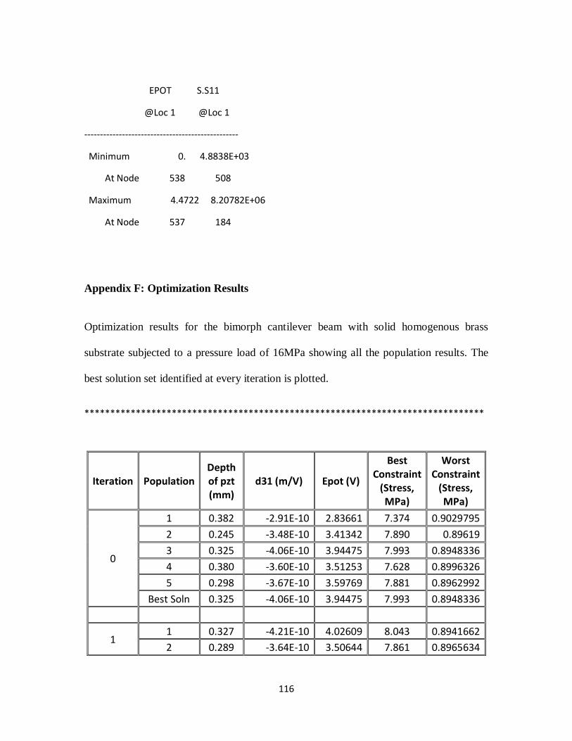
116
EPOT S.S11
@Loc 1 @Loc 1
-------------------------------------------------
Minimum 0. 4.8838E+03
At Node 538 508
Maximum 4.4722 8.20782E+06
At Node 537 184
Appendix F: Optimization Results
Optimization results for the bimorph cantilever beam with solid homogenous brass
substrate subjected to a pressure load of 16MPa showing all the population results. The
best solution set identified at every iteration is plotted.
******************************************************************************
Iteration Population Depth of pzt (mm)
d31 (m/V) Epot (V)
Best Constraint
(Stress, MPa)
Worst Constraint
(Stress, MPa)
0
1 0.382 -2.91E-10 2.83661 7.374 0.9029795
2 0.245 -3.48E-10 3.41342 7.890 0.89619
3 0.325 -4.06E-10 3.94475 7.993 0.8948336
4 0.380 -3.60E-10 3.51253 7.628 0.8996326
5 0.298 -3.67E-10 3.59769 7.881 0.8962992
Best Soln 0.325 -4.06E-10 3.94475 7.993 0.8948336
1 1 0.327 -4.21E-10 4.02609 8.043 0.8941662
2 0.289 -3.64E-10 3.50644 7.861 0.8965634
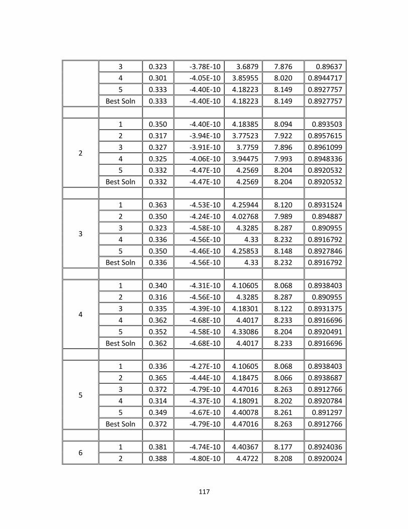
117
3 0.323 -3.78E-10 3.6879 7.876 0.89637
4 0.301 -4.05E-10 3.85955 8.020 0.8944717
5 0.333 -4.40E-10 4.18223 8.149 0.8927757
Best Soln 0.333 -4.40E-10 4.18223 8.149 0.8927757
2
1 0.350 -4.40E-10 4.18385 8.094 0.893503
2 0.317 -3.94E-10 3.77523 7.922 0.8957615
3 0.327 -3.91E-10 3.7759 7.896 0.8961099
4 0.325 -4.06E-10 3.94475 7.993 0.8948336
5 0.332 -4.47E-10 4.2569 8.204 0.8920532
Best Soln 0.332 -4.47E-10 4.2569 8.204 0.8920532
3
1 0.363 -4.53E-10 4.25944 8.120 0.8931524
2 0.350 -4.24E-10 4.02768 7.989 0.894887
3 0.323 -4.58E-10 4.3285 8.287 0.890955
4 0.336 -4.56E-10 4.33 8.232 0.8916792
5 0.350 -4.46E-10 4.25853 8.148 0.8927846
Best Soln 0.336 -4.56E-10 4.33 8.232 0.8916792
4
1 0.340 -4.31E-10 4.10605 8.068 0.8938403
2 0.316 -4.56E-10 4.3285 8.287 0.890955
3 0.335 -4.39E-10 4.18301 8.122 0.8931375
4 0.362 -4.68E-10 4.4017 8.233 0.8916696
5 0.352 -4.58E-10 4.33086 8.204 0.8920491
Best Soln 0.362 -4.68E-10 4.4017 8.233 0.8916696
5
1 0.336 -4.27E-10 4.10605 8.068 0.8938403
2 0.365 -4.44E-10 4.18475 8.066 0.8938687
3 0.372 -4.79E-10 4.47016 8.263 0.8912766
4 0.314 -4.37E-10 4.18091 8.202 0.8920784
5 0.349 -4.67E-10 4.40078 8.261 0.891297
Best Soln 0.372 -4.79E-10 4.47016 8.263 0.8912766
6 1 0.381 -4.74E-10 4.40367 8.177 0.8924036
2 0.388 -4.80E-10 4.4722 8.208 0.8920024
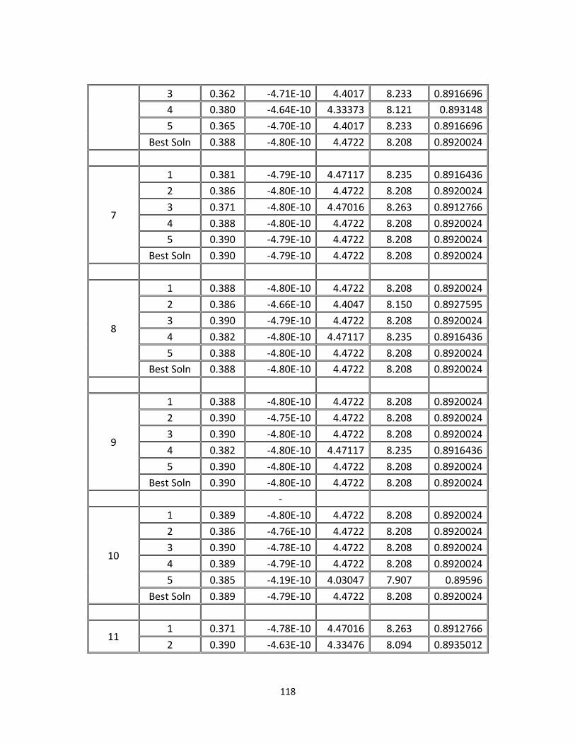
118
3 0.362 -4.71E-10 4.4017 8.233 0.8916696
4 0.380 -4.64E-10 4.33373 8.121 0.893148
5 0.365 -4.70E-10 4.4017 8.233 0.8916696
Best Soln 0.388 -4.80E-10 4.4722 8.208 0.8920024
7
1 0.381 -4.79E-10 4.47117 8.235 0.8916436
2 0.386 -4.80E-10 4.4722 8.208 0.8920024
3 0.371 -4.80E-10 4.47016 8.263 0.8912766
4 0.388 -4.80E-10 4.4722 8.208 0.8920024
5 0.390 -4.79E-10 4.4722 8.208 0.8920024
Best Soln 0.390 -4.79E-10 4.4722 8.208 0.8920024
8
1 0.388 -4.80E-10 4.4722 8.208 0.8920024
2 0.386 -4.66E-10 4.4047 8.150 0.8927595
3 0.390 -4.79E-10 4.4722 8.208 0.8920024
4 0.382 -4.80E-10 4.47117 8.235 0.8916436
5 0.388 -4.80E-10 4.4722 8.208 0.8920024
Best Soln 0.388 -4.80E-10 4.4722 8.208 0.8920024
9
1 0.388 -4.80E-10 4.4722 8.208 0.8920024
2 0.390 -4.75E-10 4.4722 8.208 0.8920024
3 0.390 -4.80E-10 4.4722 8.208 0.8920024
4 0.382 -4.80E-10 4.47117 8.235 0.8916436
5 0.390 -4.80E-10 4.4722 8.208 0.8920024
Best Soln 0.390 -4.80E-10 4.4722 8.208 0.8920024
-
10
1 0.389 -4.80E-10 4.4722 8.208 0.8920024
2 0.386 -4.76E-10 4.4722 8.208 0.8920024
3 0.390 -4.78E-10 4.4722 8.208 0.8920024
4 0.389 -4.79E-10 4.4722 8.208 0.8920024
5 0.385 -4.19E-10 4.03047 7.907 0.89596
Best Soln 0.389 -4.79E-10 4.4722 8.208 0.8920024
11 1 0.371 -4.78E-10 4.47016 8.263 0.8912766
2 0.390 -4.63E-10 4.33476 8.094 0.8935012

119
3 0.389 -4.80E-10 4.4722 8.208 0.8920024
4 0.376 -4.80E-10 4.47117 8.235 0.8916436
5 0.386 -4.76E-10 4.4722 8.208 0.8920024
Best Soln 0.386 -4.76E-10 4.4722 8.208 0.8920024
12
1 0.374 -4.77E-10 4.47016 8.263 0.8912766
2 0.389 -4.80E-10 4.4722 8.208 0.8920024
3 0.386 -4.76E-10 4.4722 8.208 0.8920024
4 0.390 -4.80E-10 4.4722 8.208 0.8920024
5 0.377 -4.80E-10 4.47117 8.235 0.8916436
Best Soln 0.390 -4.80E-10 4.4722 8.208 0.8920024
13
1 0.386 -4.77E-10 4.4722 8.208 0.8920024
2 0.363 -4.80E-10 4.46919 8.291 0.890904
3 0.386 -4.28E-10 4.1107 7.932 0.8956284
4 0.389 -4.69E-10 4.4047 8.150 0.8927595
5 0.386 -4.68E-10 4.4047 8.150 0.8927595
Best Soln 0.386 -4.77E-10 4.4722 8.208 0.8920024
14
1 0.390 -4.38E-10 4.1877 7.985 0.8949361
2 0.389 -4.75E-10 4.4047 8.150 0.8927595
3 0.365 -4.70E-10 4.4017 8.233 0.8916696
4 0.389 -4.66E-10 4.4047 8.150 0.8927595
5 0.388 -4.56E-10 4.33476 8.094 0.8935012
Best Soln 0.386 -4.77E-10 4.4722 8.208 0.8920024
15
1 0.387 -4.80E-10 4.4722 8.208 0.8920024
2 0.387 -4.80E-10 4.4722 8.208 0.8920024
3 0.380 -4.78E-10 4.47117 8.235 0.8916436
4 0.359 -4.59E-10 4.33177 8.176 0.8924192
5 0.386 -4.27E-10 4.1107 7.932 0.8956284
Best Soln 0.387 -4.80E-10 4.4722 8.208 0.8920024
16 1 0.368 -4.76E-10 4.47016 8.263 0.8912766
2 0.348 -4.80E-10 4.46826 8.320 0.8905287

120
3 0.390 -4.6229E-10 4.33476 8.094 0.8935012
4 0.389 -4.66E-10 4.4047 8.150 0.8927595
5 0.387 -4.71E-10 4.4047 8.150 0.8927595
Best Soln 0.387 -4.80E-10 4.4722 8.208 0.8920024
17
1 0.376 -4.71E-10 4.40367 8.177 0.8924036
2 0.389 -4.80E-10 4.4722 8.208 0.8920024
3 0.387 -4.80E-10 4.4722 8.208 0.8920024
4 0.388 -4.80E-10 4.4722 8.208 0.8920024
5 0.388 -4.80E-10 4.4722 8.208 0.8920024
Best Soln 0.389 -4.80E-10 4.4722 8.208 0.8920024
18
1 0.347 -4.80E-10 4.46826 8.320 0.8905287
2 0.389 -4.80E-10 4.4722 8.208 0.8920024
3 0.375 -4.80E-10 4.47016 8.263 0.8912766
4 0.388 -4.80E-10 4.4722 8.208 0.8920024
5 0.388 -4.80E-10 4.4722 8.208 0.8920024
Best Soln 0.388 -4.80E-10 4.4722 8.208 0.8920024
19
1 0.388 -4.65E-10 4.4047 8.150 0.8927595
2 0.355 -4.80E-10 4.46919 8.291 0.890904
3 0.390 -4.80E-10 4.4722 8.208 0.8920024
4 0.389 -4.59E-10 4.33476 8.094 0.8935012
5 0.387 -4.80E-10 4.4722 8.208 0.8920024
Best Soln 0.388 -4.80E-10 4.4722 8.208 0.8920024