DesignofExperiment - molekuelwald.square7.chmolekuelwald.square7.ch/biblio/Industrielle Chemie Praktikum/ICP... · In ideal solutions the freezing point depression is a function of

Zurich University of Applied Sciences

Departement N

Practical Industrial Chemistry

HS13-G03

Design of ExperimentOptimisation of a Frigorific Mixture

Autoren:

Tobias MollDominik Bachmann

Dozent:

Dr. Achim Ecker

autumn semester 20132nd December 2014


1. Assignment of Tasks

1.1. Objective• A frigorific mixture is to be optimized at -25 ◦C using GlobalOptimize software.

- Finde a mixture of ice, ethanol and sodium chloride cooling to −25 ◦C ±0.5 ◦C.

• Optimize the price of the frigorific mixture using GlobalOptimize software.

Copolymerisation 2


2. Theoretical Part

2.1. State Transition Points of Pure SubstancesThe process of melting a state transition from solid to liquid. The potential energy hoding the crystaltogether must be overcome by adding heat to it [1]. The substances are not being atomized, not allbonds are being broken. Meltingpoints from different substances may vary widely. This is due to theirdifference in intermolecular interactions. Substances with a relatively deep melting point are beinghold together by London dispersion forces only. table 2.1 some substances with melting points, mostlycaused by London dispersion forces, are listed.

Table 2.1. – List of substances with low melting point and boiling point [2] [1].Substance Melting point / K Boiling point / K

Methane 90.681 111.6681

Boron trifluoride 146.28 1 172 2

Tetrachloromethane 250.89 1 349.95 1

Comparing the melting and boiling point of Methane with those of Tetrachloromethane, differences of160 K (melting points) respectively 240 K (boiling points) are being found. This is due to the greaterpolarizability of Tetrachloromethane, stabilizing an uneven charge distribution better than Methane.Permanent dipoles also have a great influence on melting and boiling points. Polar substances, such aswater, Sulphuric acid or Chloroform build Hydrogen bonds in liquid state, representing a great deal oftheir boiling points. The bonds in salts are even more polar than the Hydrogen bonds, thus they haveeven higher melting points [1].

2.2. Colligative PropertiesColligative Properties are the effects a solute has on its solvent. In this work, osmotic pressure andsolubility are not of significant interest and therefore not discussed any further, although they arebeing lined among the colligative properties.The chemical potential of a solvent is, relative to the pure solvent, being decreased by solutes. Becausestate transition temperatures always occur at an equilibrium in chemical potential of two physical states(µ(l) = µs [3] for the freezing point), the state transition temperature changes. As a simplification, it isassumed that the solvent is non volatile and, when freezing the solvent grows in pure crystals. Thisleads to a change of the chemical potential in liquid state.

2.2.0.1. Freezing-Point Depression

The freezing-point depression can be calculated with the following equation

µ = µ∗A +RT ln xA (2.1)

where xA corresponds to the mole fraction of the solvent. Comparing the freezing point of pure waterand the freezing point of sodium cloride solution, the freezing point of the solution will decrease with

Copolymerisation 3


an increasing concentration of sodium chloride. In [2] a table with different concentrations of sodiumchloride solutions from 0.086 mol L−1 (∆T = 0.3 ◦C) to 4.382 mole/L (∆T = 19.18 ◦C) is available.This effect is being used on icy streets in winter to melt the ice without heating it. It is furtherly usedin cooling baths to create a constant and low temperature. This is highly convenient, since the meltingenergy from ice can be used to cool the solution below freezing temperature of pure watersection 2.3on page 4. The energy consuming creation and storage of liquid nitrogen or carbono dioxide can bereduced.In ideal solutions the freezing point depression is a function of only two parameters, namely theCryoscopic Constant and the mole fraction of the solute [3].

∆Tf = EfxB (2.2)

Ef is the Cryoscopic Constant [3]. It is a characteristic property of a solvent and can be calculated asin equation 2.3 on page 4

Ef =RT ∗2

f

∆smH(2.3)

2.3. Frigorific MixturesFrigorific mixtures are usually mixtures of two or three components: A solvent, which may also bethe cooling agent, an additive (decreasing the chemical potential) and a compulsory solvent. Thecooling system is based on the melting enthalpy of ice (sometimes even sublimation enthalpy of dryice), draining heat energy from the liquid phase and by that cooling it down. The additive depressesthe freezing point of the solvent (water may be used as solvent while ice is being used as a cooling agentdue to the collegative properties as described in section 2.2 on page 3). Depending on the mole fractionof the solvent, the solvent itself and the additional solvent (ethanol for example) the freezing-pointdepression will vary.

2.4. Design of experimentsIn process technology, parameters are set for an optimal process. This can relate to maximum putthrough, maximal purity and selectivity, minimum reaction time or minimal process costs. Sincevarious parameters can be changed in a process, for example concentrations, catalyst, pressure,temperature, an array with all influence seizes is being defined as well as an array with target seizes.Since varying the influence seizes in order to model the complete space by an array experiment israther time-consuming, this is made by a design program (here GlobalOptimize). Depending on themathematical proportionality and the number of influence seizes, a minimum number of experiments isbeing made to model the space. The results build the input for modelling the space roughly. Afterthat, an approximation to the influence seize omptima is made. GO uses a newton method for findingintercept points. Every approximation leads to a new experiment with new parameters. If the result isunsatisfying, a new experiment is being set up by a new approximation. To generate valid lab data itis therefore crucial to maintain a stable process with no other influences.In this experiment, the mole fractions of ice, ethanol and sodium chloride are influence seizes. Thetarget seizes are cooling temperature (-25 ◦C) and minimum price.

Copolymerisation 4


3. Procedure and Accomplishments

3.1. GlobalOptimize (GO!)For the optimization of the frigorific mixture the commercial software GlobalOptimize V2.0.1 (profes-sional) (GO!)[4] was used.The chosen way to optimize the frigorific mixture was experiment design without expert knowledge.

3.2. ExperimentsFirst, the maximal moles of each substance in use were defined. These were 0.5 to 0.97 mole for ice,0.01 to 0.4 mole for ethanol and 0.01 to 0.1 mole for NaCl. As described in section 3.1 nine differentmeasurements were proposed. There were two extra experiments made during the system test whereofthe results also were used. The recommended mixture ratio are shown in table 3.1.

Table 3.1. – By GO! recommended mixture ratio. Two extra measurements were made. The limitswere 0.5 to 0.97 mole for ice, 0.01 to 0.4 mole for ethanol and 0.01 to 0.1 mole forNaCl. The sum was calculated to normalize the experimental mixture

Number Ice/ mol Ethanol/ mol NaCl/ mol Sum/ mol

No. 1 0.735 0.205 0.055 0.995No. 2 0.500 0.400 0.010 0.910No. 3 0.500 0.400 0.100 1.000No. 4 0.970 0.010 0.010 0.990No. 5 0.970 0.400 0.010 1.380No. 6 0.970 0.400 0.100 1.470No. 7 0.500 0.010 0.010 0.520No. 8 0.500 0.010 0.100 0.610No. 9 0.970 0.010 0.100 1.080Extra 1 0.970 0.400 0.055 1.425Extra 2 0.735 0.100 0.100 0.935

These data were converted to get normalized ratio in gram or millilitre (compare equation 3.1 on page5 and equation 3.2 on page 5 especially for ethanol). The normalization was made so the final amountof substance of the frigorific mixture is always the same what makes the results comparable.

(mole of ingredient) · (molecular weight) · (total moles in the mixture)(sum of mole for these mixture) (3.1)

(mole of ingredient) · (molecular weight) · (total moles in the mixture)(sum of mole for these mixture) · (density of ethnol) (3.2)

The total moles in the final mixture were fixed at 18 moles. This number was chosen arbitrarily butthe amount has to top an undefined minimum to get a final mass of frigorific mixture which is easily

Copolymerisation 5


to handle. The converted and normalised data are shown in table 3.2 on page 6. The amount of eachsubstance were not weighted with an analytical precision, still the error is 1 % at a maximum.

3.3. Test set-up3.3.1. Negative MeasurementsAt the beginning of the experiment different test set-ups were tested to find a stable one. As describedin section 2.4 on page 4 it is important that each experiment is running under controlled condition andthe final value should not be able to vary too easily. The first measurements were made as describedas follows. The components were blended in a beaker and stirred for 20 seconds with a mechanicstirrer (see figure 3.1 on page 7). Afterwards the mixture was transferred into a Dewar vessel to workin a thermally isolated system. The temperature was measured after 2 minutes. The problem wasthat, whenever the mixture was stirred or even moved a little (inserting the thermometer was shockenough), the temperature fell. This showed that the experiment is not stable. Determining if theset-up produced valid data the first experiments were made as a multiple determination. The resultingdata were varying up to 5 ◦C. The method was inadequate.

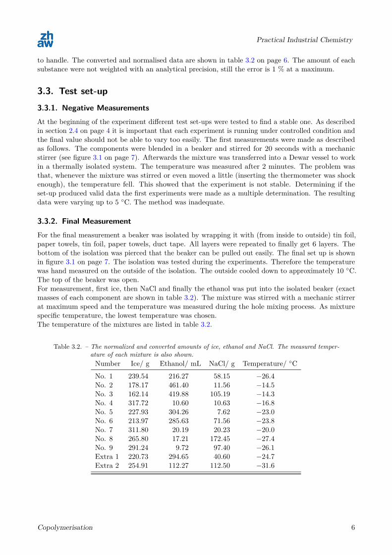
3.3.2. Final MeasurementFor the final measurement a beaker was isolated by wrapping it with (from inside to outside) tin foil,paper towels, tin foil, paper towels, duct tape. All layers were repeated to finally get 6 layers. Thebottom of the isolation was pierced that the beaker can be pulled out easily. The final set up is shownin figure 3.1 on page 7. The isolation was tested during the experiments. Therefore the temperaturewas hand measured on the outside of the isolation. The outside cooled down to approximately 10 ◦C.The top of the beaker was open.For measurement, first ice, then NaCl and finally the ethanol was put into the isolated beaker (exactmasses of each component are shown in table 3.2). The mixture was stirred with a mechanic stirrerat maximum speed and the temperature was measured during the hole mixing process. As mixturespecific temperature, the lowest temperature was chosen.The temperature of the mixtures are listed in table 3.2.

Table 3.2. – The normalized and converted amounts of ice, ethanol and NaCl. The measured temper-ature of each mixture is also shown.Number Ice/ g Ethanol/ mL NaCl/ g Temperature/ ◦C

No. 1 239.54 216.27 58.15 −26.4No. 2 178.17 461.40 11.56 −14.5No. 3 162.14 419.88 105.19 −14.3No. 4 317.72 10.60 10.63 −16.8No. 5 227.93 304.26 7.62 −23.0No. 6 213.97 285.63 71.56 −23.8No. 7 311.80 20.19 20.23 −20.0No. 8 265.80 17.21 172.45 −27.4No. 9 291.24 9.72 97.40 −26.1Extra 1 220.73 294.65 40.60 −24.7Extra 2 254.91 112.27 112.50 −31.6

Copolymerisation 6


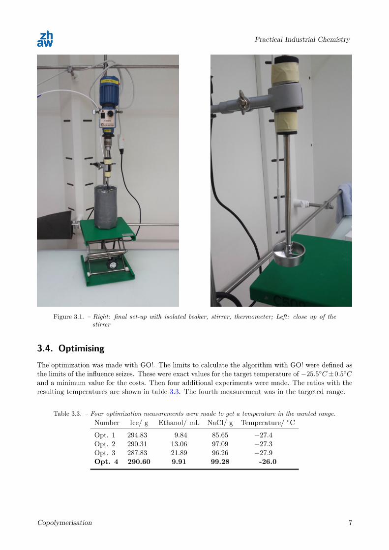
Figure 3.1. – Right: final set-up with isolated beaker, stirrer, thermometer; Left: close up of thestirrer

3.4. OptimisingThe optimization was made with GO!. The limits to calculate the algorithm with GO! were defined asthe limits of the influence seizes. These were exact values for the target temperature of −25.5◦C±0.5◦Cand a minimum value for the costs. Then four additional experiments were made. The ratios with theresulting temperatures are shown in table 3.3. The fourth measurement was in the targeted range.

Table 3.3. – Four optimization measurements were made to get a temperature in the wanted range.Number Ice/ g Ethanol/ mL NaCl/ g Temperature/ ◦C

Opt. 1 294.83 9.84 85.65 −27.4Opt. 2 290.31 13.06 97.09 −27.3Opt. 3 287.83 21.89 96.26 −27.9Opt. 4 290.60 9.91 99.28 -26.0

Copolymerisation 7


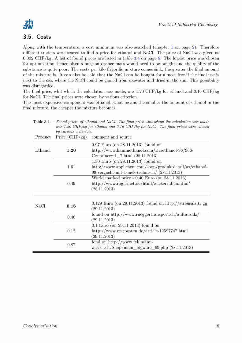
3.5. CostsAlong with the temperature, a cost minimum was also searched (chapter 1 on page 2). Thereforedifferent traders were seared to find a price for ethanol and NaCl. The price of NaCl was given as0.002 CHF/kg. A list of found prices are listed in table 3.4 on page 8. The lowest price was chosenfor optimization, hence often a huge substance mass would need to be bought and the quality of thesubstance is quite poor. The costs per kilo frigorific mixture comes sink, the greater the final amountof the mixture is. It can also be said that the NaCl can be bought for almost free if the final use isnext to the sea, where the NaCl could be gained from seawater and dried in the sun. This possibilitywas disregarded.The final price, whit which the calculation was made, was 1.20 CHF/kg for ethanol and 0.16 CHF/kgfor NaCl. The final prices were chosen by various criterion.The most expensive component was ethanol, what means the smaller the amount of ethanol in thefinal mixture, the cheaper the mixture becomes.

Table 3.4. – Found prices of ethanol and NaCl. The final price whit whom the calculation was madewas 1.20 CHF/kg for ethanol and 0.16 CHF/kg for NaCl. The final prices were chosenby various criterion.

Product Price (CHF/kg) comment and source

Ethanol 1.200.97 Euro (on 28.11.2013) found onhttp://www.kaminethanol.com/Bioethanol-96/966-Container:::1_7.html (28.11.2013)

1.611.30 Euro (on 28.11.2013) found onhttp://www.applichem.com/shop/produktdetail/as/ethanol-99-vergaellt-mit-1-mek-technisch/ (28.11.2013)

0.49World marked price - 0.40 Euro (on 28.11.2013)http://www.roglernet.de/html/zuckerruben.html"(28.11.2013)

NaCl 0.16 0.129 Euro (on 29.11.2013) found on http://streusalz.tr.gg(29.11.2013)

0.46 found on http://www.rueggertransport.ch/auftausalz/(29.11.2013)

0.120.1 Euro (on 29.11.2013) found onhttp://www.restposten.de/article-12597747.html(29.11.2013)

0.87 fond on http://www.fehlmann-wasser.ch/Shop/main_bigware_69.php (28.11.2013)

Copolymerisation 8


4. Results

As described in section 3.4 on page 7 a mixture optimum was found with a ratio of 0.95 mole ice, 0.01mole ethanol and 0.1 mole NaCl. The cost for this ratio is 0.0284 CHF/kg. There were two equationsfound which describe the relation between component ratio and temperature (y1 in equation 4.2 onpage 9) and the relation of components ratio and costs (y2 in equation 4.3 on page 9). x1, x2, x3 arethe molar ratio of ice, ethanol and NaCl in the mixture. For both correlations a full quadratic equationwas found.

y1 = −78.18x1 + 57.684x21 + 15.149x2 + 61.855x2

2 − 122.99x3 + 458.31x23 (4.1)

−59.541x1x2 − 41.198x1x3 + 244.49x2x3 + 6.476

y2 = 0.07197x1 − 0.07503x21 + 2.0648x2 − 0.70356x2

2 + 0.046876x3 + 0.31473x23 (4.2)

−0.86745x1x2 + 0.13472x1x3 − 1.1034x2x3 − 0.0022379

The correlations were recalculated with Excel to check if the equation is correct (see also section 5.1 onpage 12 and section 5.4 on page 13).

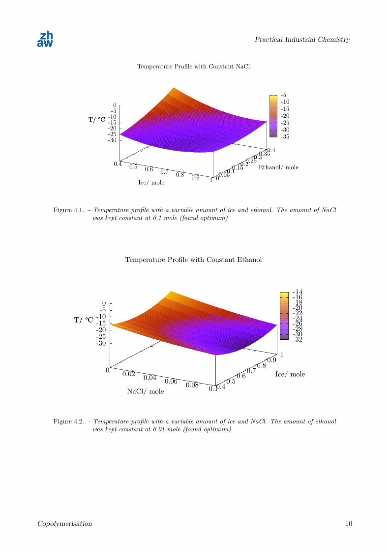
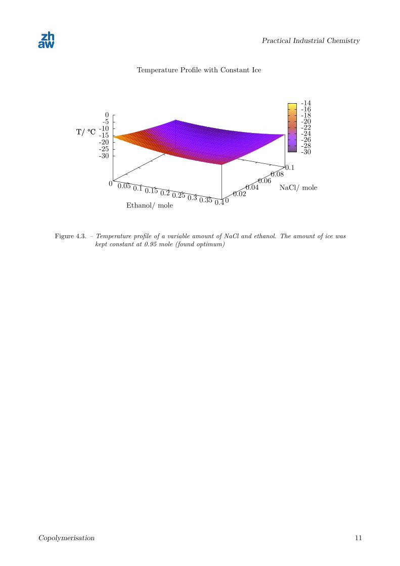
4.1. 3D-PlotsIn these sections three plots were shown (see figure 4.1 on page 10, figure 4.2 on page 10 and figure 4.3on page 11). In each was one influence seize kept constant at the found optimum. The temperature isdepending on the variation of the other two influence sizes.

Copolymerisation 9


0.4 0.5 0.6 0.7 0.8 0.9 1 00.050.10.15

0.20.250.30.35

0.4-30-25-20-15-10-50

T/ °C

Temperature Profile with Constant NaCl

Ice/ mole

Ethanol/ mole

T/ °C

-35-30-25-20-15-10-5

Figure 4.1. – Temperature profile with a variable amount of ice and ethanol. The amount of NaClwas kept constant at 0.1 mole (found optimum)

0 0.02 0.04 0.06 0.08 0.10.40.5

0.60.7

0.80.9

1-30-25-20-15-10-50

T/ °C

Temperature Profile with Constant Ethanol

NaCl/ mole

Ice/ mole

T/ °C

-32-30-28-26-24-22-20-18-16-14

Figure 4.2. – Temperature profile with a variable amount of ice and NaCl. The amount of ethanolwas kept constant at 0.01 mole (found optimum)

Copolymerisation 10


0 0.05 0.1 0.15 0.2 0.25 0.3 0.35 0.400.02

0.040.06

0.080.1

-30-25-20-15-10-50

T/ °C

Temperature Profile with Constant Ice

Ethanol/ mole

NaCl/ mole

T/ °C

-30-28-26-24-22-20-18-16-14

Figure 4.3. – Temperature profile of a variable amount of NaCl and ethanol. The amount of ice waskept constant at 0.95 mole (found optimum)

Copolymerisation 11


5. Discussion

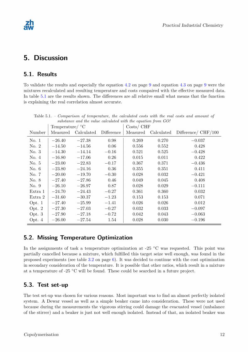
5.1. ResultsTo validate the results and especially the equation 4.2 on page 9 and equation 4.3 on page 9 were themixtures recalculated and resulting temperature and costs compaired with the effective measured data.In table 5.1 are the results shown. The differences are all relative small what means that the functionis explaining the real correlation almost accurate.

Table 5.1. – Comparison of temperature, the calculated costs with the real costs and amount ofsubstance and the value calculated with the equation from GO!

Temperature/ ◦C Costs/ CHFNumber Measured Calculated Difference Measured Calculated Difference/ CHF/100

No. 1 −26.40 −27.38 0.98 0.269 0.270 −0.037No. 2 −14.50 −14.56 0.06 0.556 0.552 0.428No. 3 −14.30 −14.14 −0.16 0.521 0.525 −0.428No. 4 −16.80 −17.06 0.26 0.015 0.011 0.422No. 5 −23.00 −22.83 −0.17 0.367 0.371 −0.436No. 6 −23.80 −24.16 0.36 0.355 0.351 0.411No. 7 −20.00 −19.70 −0.30 0.028 0.032 −0.421No. 8 −27.40 −27.86 0.46 0.049 0.045 0.408No. 9 −26.10 −26.97 0.87 0.028 0.029 −0.111Extra 1 −24.70 −24.43 −0.27 0.361 0.360 0.032Extra 2 −31.60 −30.37 −1.23 0.153 0.153 0.071Opt. 1 −27.40 −25.99 −1.41 0.026 0.026 0.012Opt. 2 −27.30 −27.03 −0.27 0.032 0.033 −0.097Opt. 3 −27.90 −27.18 −0.72 0.042 0.043 −0.063Opt. 4 −26.00 −27.54 1.54 0.028 0.030 −0.196

5.2. Missing Temperature OptimizationIn the assignments of task a temperature optimization at -25 ◦C was requested. This point waspartially cancelled because a mixture, which fulfilled this target seize well enough, was found in theproposed experiments (see table 3.2 on page 6). It was decided to continue with the cost optimizationin secondary consideration of the temperature. It is possible that other ratios, which result in a mixtureat a temperature of -25 ◦C will be found. These could be searched in a future project.

5.3. Test set-upThe test set-up was chosen for various reasons. Most important was to find an almost perfectly isolatedsystem. A Dewar vessel as well as a simple beaker came into consideration. These were not usedbecause during the measurements the vigorous stirring could damage the evacuated vessel (unbalanceof the stirrer) and a beaker is just not well enough isolated. Instead of that, an isolated beaker was

Copolymerisation 12


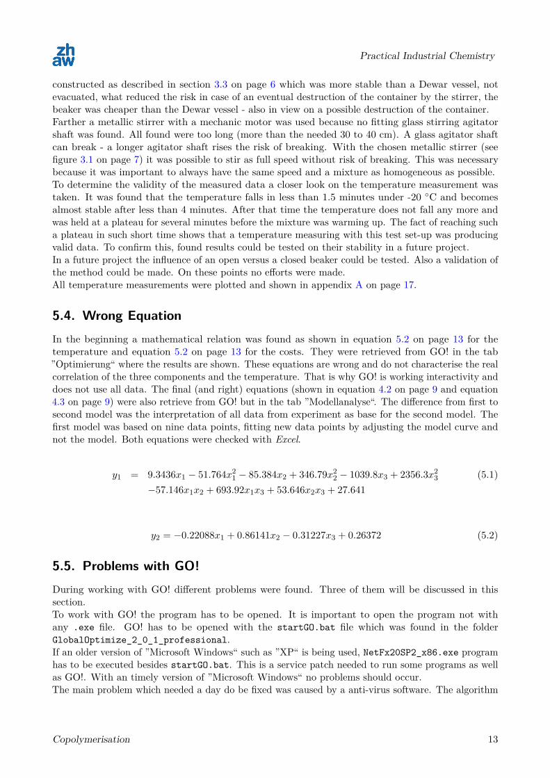
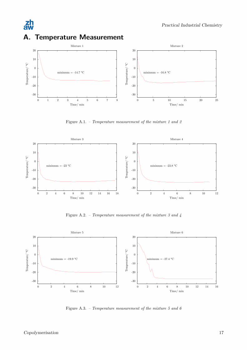
constructed as described in section 3.3 on page 6 which was more stable than a Dewar vessel, notevacuated, what reduced the risk in case of an eventual destruction of the container by the stirrer, thebeaker was cheaper than the Dewar vessel - also in view on a possible destruction of the container.Farther a metallic stirrer with a mechanic motor was used because no fitting glass stirring agitatorshaft was found. All found were too long (more than the needed 30 to 40 cm). A glass agitator shaftcan break - a longer agitator shaft rises the risk of breaking. With the chosen metallic stirrer (seefigure 3.1 on page 7) it was possible to stir as full speed without risk of breaking. This was necessarybecause it was important to always have the same speed and a mixture as homogeneous as possible.To determine the validity of the measured data a closer look on the temperature measurement wastaken. It was found that the temperature falls in less than 1.5 minutes under -20 ◦C and becomesalmost stable after less than 4 minutes. After that time the temperature does not fall any more andwas held at a plateau for several minutes before the mixture was warming up. The fact of reaching sucha plateau in such short time shows that a temperature measuring with this test set-up was producingvalid data. To confirm this, found results could be tested on their stability in a future project.In a future project the influence of an open versus a closed beaker could be tested. Also a validation ofthe method could be made. On these points no efforts were made.All temperature measurements were plotted and shown in appendix A on page 17.

5.4. Wrong EquationIn the beginning a mathematical relation was found as shown in equation 5.2 on page 13 for thetemperature and equation 5.2 on page 13 for the costs. They were retrieved from GO! in the tab”Optimierung“ where the results are shown. These equations are wrong and do not characterise the realcorrelation of the three components and the temperature. That is why GO! is working interactivity anddoes not use all data. The final (and right) equations (shown in equation 4.2 on page 9 and equation4.3 on page 9) were also retrieve from GO! but in the tab ”Modellanalyse“. The difference from first tosecond model was the interpretation of all data from experiment as base for the second model. Thefirst model was based on nine data points, fitting new data points by adjusting the model curve andnot the model. Both equations were checked with Excel.

y1 = 9.3436x1 − 51.764x21 − 85.384x2 + 346.79x2

2 − 1039.8x3 + 2356.3x23 (5.1)

−57.146x1x2 + 693.92x1x3 + 53.646x2x3 + 27.641

y2 = −0.22088x1 + 0.86141x2 − 0.31227x3 + 0.26372 (5.2)

5.5. Problems with GO!During working with GO! different problems were found. Three of them will be discussed in thissection.To work with GO! the program has to be opened. It is important to open the program not withany .exe file. GO! has to be opened with the startGO.bat file which was found in the folderGlobalOptimize_2_0_1_professional.If an older version of ”Microsoft Windows“ such as ”XP“ is being used, NetFx20SP2_x86.exe programhas to be executed besides startGO.bat. This is a service patch needed to run some programs as wellas GO!. With an timely version of ”Microsoft Windows“ no problems should occur.The main problem which needed a day do be fixed was caused by a anti-virus software. The algorithm

Copolymerisation 13


of GO! was identified as malware and was urgently deleted. The algorithm alGO.exe should bein the folder \GlobalOptimize_2_0_1_professional\GO\plugins\ch.fhsg.nc.go.engine.matlab.The file was restored what fixed the error and the anti-virus software was deactivated during the workwith GO!. The used anti-virus software was ”avast¡‘. The problem was solved independently withtelephone support from the producer.

Copolymerisation 14


Bibliography

[1] J.E. Huheey, E.A. Keiter, R. Keiter, and R. Steudel. Anorganische Chemie: Prinzipien von Strukturund Reaktivität. De Gruyter, 2003.

[2] W.M. Haynes. CRC Handbook of Chemistry and Physics, 94th Edition. CRC Handbook ofChemistry and Physics. Taylor & Francis Limited, 2013.

[3] P.W. Atkins, J. De Paula, and M. Bär. Physikalische Chemie: 4. Auflage. Number Bd. 1. Wiley-VCHVerlag GmbH, 2006.

[4] FHS St.Gallen. GlobalOptimize. http://www.globaloptimize.ch developer website.

Copolymerisation 15


Appendices

Copolymerisation 16


A. Temperature Measurement

-30

-20

-10

0

10

20

0 1 2 3 4 5 6 7 8

Tempe

rature/

°C

Time/ min

Mixture 1

minimum = -14.7 °C

-30

-20

-10

0

10

20

0 5 10 15 20 25

Tempe

rature/

°C

Time/ min

Mixture 2

minimum = -16.8 °C

Figure A.1. – Temperature measurement of the mixture 1 and 2

-30

-20

-10

0

10

20

0 2 4 6 8 10 12 14 16 18

Tempe

rature/

°C

Time/ min

Mixture 3

minimum = -23 °C

-30

-20

-10

0

10

20

0 2 4 6 8 10 12

Tempe

rature/

°C

Time/ min

Mixture 4

minimum = -23.8 °C


-30

-20

-10

0

10

20

0 2 4 6 8 10 12

Tempe

rature/

°C

Time/ min

Mixture 5

minimum = -19.9 °C

-30

-20

-10

0

10

20

0 2 4 6 8 10 12 14 16

Tempe

rature/

°C

Time/ min

Mixture 6

minimum = -27.4 °C


Copolymerisation 17


-30

-20

-10

0

10

20

0 2 4 6 8 10 12 14

Tempe

rature/

°C

Time/ min

Mixture 7

minimum = -26.1 °C

-30

-20

-10

0

10

20

0 5 10 15 20 25

Tempe

rature/

°C

Time/ min

Mixture 8

minimum = -24.7 °C


-30

-20

-10

0

10

20

0 2 4 6 8 10 12 14 16

Tempe

rature/

°C

Time/ min

Mixture 9

minimum = -31.6 °C

-30

-20

-10

0

10

20

1 2 3 4 5 6 7 8 9 10

Tempe

rature/

°C

Time/ min

Extra Mixture 1

minimum = -26.4 °C

Figure A.5. – Temperature measurement of the mixture 9 and extra mixture 1

-30

-20

-10

0

10

20

1 2 3 4 5 6 7 8 9

Tempe

rature/

°C

Time/ min

Extra Mixture 1

minimum = -14.6 °C

-30

-20

-10

0

10

20

0 5 10 15 20 25

Tempe

rature/

°C

Time/ min

Optimization Mixture 1

minimum = -27.45 °C

Figure A.6. – Temperature measurement of the extra mixture 1 and the optimization mixture 1

Copolymerisation 18


-30

-20

-10

0

10

20

0 2 4 6 8 10 12 14 16

Tempe

rature/

°C

Time/ min



-30

-20

-10

0

10

20

0 2 4 6 8 10 12 14 16 18

Tempe

rature/

°C

Time/ min



Figure A.7. – Temperature measurement of the optimization mixture 2 and the optimization mixture3

-30

-20

-10

0

10

20

0 2 4 6 8 10 12 14

Tempe

rature/

°C

Time/ min



Figure A.8. – Temperature measurement of the optimization mixture 4

Copolymerisation 19

PracticalIndustrialChem

istryB. Chemicals

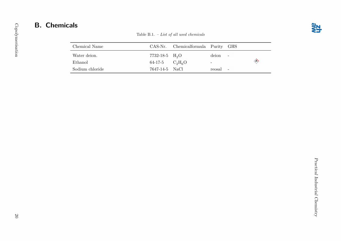
Table B.1. – List of all used chemicals

Chemical Name CAS-Nr. Chemicalformula Purity GHS

Water deion. 7732-18-5 H2O deion -Ethanol 64-17-5 C2H6O -Sodium chloride 7647-14-5 NaCl reosal -

Copolym

erisation20

Documents

DesignofExperiment - molekuelwald.square7.chmolekuelwald.square7.ch/biblio/Industrielle Chemie Praktikum/ICP... · In ideal solutions the freezing point depression is a function of